Highland Areas in the Digital Era: From Abyss to Quatum. European Mountain Series Forecasting (10)

1. Introduction and Literature Review

Regarding organizations and their structuring, it is acknowledged that ICT presents various structural forms that contribute to enhancing organizational capability and performance, as well as to controlling and monitoring outcomes. The results indicate that ICT addresses both ICT governance and governance through ICT. Other emerging themes include the role of ICT in improving outcomes in intra- and inter-organizational relationships. (Wilkin & Chenhall, 2020)

Concerning long-term economic growth prospects, it is implied that one of the primary economic perspectives on the innovative impact of ICT in society suggests that the tendency toward stagnation is a consequence of resistance to digital change. The study of stagnation has a long history, but the most significant research pertains to economic growth in the context of diminishing resources and resistance to changes in digital society in mountain areas. (Nordhaus, 2021)

ICT has significantly altered human existence, with mountain areas being the most favored through digital applications at the societal level. Mountain regions, especially urban ones, intensively apply the Internet of Things (IoT), Internet of Drones (IoD), and Internet of Vehicles (IoV). Smart cities can become part of the solution for mountain development, particularly through intelligent public and private governance. The Internet of Everything (IoE) can have a major impact on people’s lifestyles, with mountain areas requiring such digital infusions. (Heidari et al., 2022)

Recent discoveries in the field of information and communications advance interconnected information processing systems by leveraging the potentials of quantum information. Particularly necessary in mountain areas, quantum information systems enable the transfer of information between disparate physical environments. Thus, digital implementation becomes much easier through the sharing of quantum information via various nodes and arcs in constant dynamics. Among the arcs and nodes of the quantum system, which can ensure high marginal sustainability for mountain areas, are semiconductor electronics, individual atoms from the surrounding environment, light pulses in optical fibers, or microwave fields. Quantum interconnections can ensure enhanced sustainability for mountain areas by allowing high permissiveness in the transfer of quantum states. However, there are alarm signals regarding fragile quantum states between different physical parts or degrees of freedom of the system, especially in mountain spaces. The diversity of quantum platforms (superconducting, atomic, solid-state color centers, transparent, optical, etc.) will form a “quantum internet,” and mountain areas will emerge as the biggest beneficiaries of this challenge. Quantum society will face the same issues as internet society and the Internet of Everything society, namely losses in the nodes or arcs of the system. Additionally, in mountain areas, quantum systems, which will scale to large dimensions, will encounter the same types of inherent interconnection blockages, especially in quantum interconnections. The explicit reference here pertains to signal attenuation due to various blockages encountered in mountain areas, such as mountain altitude, vegetation density, etc. (More information can be found in the article “Mountain Precision Agriculture Index: A Review” - [https://www.preprints.org/manuscript/202501.1104/v2]). Considering the possibility of diversifying quantum platforms, materials used, applications, and necessary infrastructure, convergent research programs for the mountain patterns of the world are required. The vulnerability of quantum information security currently hinders the global propagation of quantum systems. Mountain areas could become vectors of quantum interconnection by transforming into real implementation models.

The challenges related to connecting different parts of the system in quantum networks maintain the same structural entanglement, although the degree of complexity becomes superior. Quantum networks are of particular interest for mountain areas, especially in the context of long-distance communication, managing to stabilize, distribute, and maintain informational load over thousands of kilometers. This becomes relevant in the case of inevitable signal losses within communication channels. In this context, the importance of modular quantum computing schemes is emphasized, probably the only viable approach to ensuring total safety of quantum systems. The presented study shows that the quantum future depends on interdisciplinarity focused on developing scalable integrated quantum photonic platforms by including emerging quantum materials, manufacturing and packaging integrated quantum photonic devices, and developing optical fibers with nano-measurable losses. The hardware components of the quantum system must gradually become convergent, primarily referring to optical compression modules, frequency conversion modules, entanglement sources, transducers, sensors, detectors, lasers. The extra- and intra-systemic divergence at the software and hardware levels must be translated into convergence so that quantum systems, especially those applied to mountain areas, ensure evolutionary contiguity. (Awschalom et al., 2021)

From the perspective of implementing ICT for Open Innovation (OI), two types of capabilities can be distinguished: strategic — which must be developed so that the organization can benefit from a proactive OI strategy — and operational — for the efficient implementation of OI processes. At the strategic level, ICT ensures dynamic capabilities and cognitive processes related to managerial staff who can develop and utilize an appropriate level of absorptive capacity and active transparency. At the operational level, ICT supports the improvement of daily performance of OI activities. From this perspective, collaboration and complex data analysis in organizational processes related to OI are addressed. Based on organizational capabilities, ICT can be discussed as a factor for improving the strategic and operational processes of OI. The complexity of these two types of processes requires customized approaches. While strategic processes are creative, complex, and subjective — their automation being almost impossible — operational processes are supported through user coding, aggregation, and computability related to machine reasoning and data processing. (Adamides & Karacapilidis, 2020)

Aligned with the previously presented research, the study by Liu et al. (2020) ensures the gradual transition from the 5G mobile network (2019) to 6G (2030). To pave the way for the development of the sixth-generation mobile network (6G), the vision and requirements must first be identified to facilitate the identification of key technologies and the design of a comprehensive system. The presented article first identifies the vision for societal development by 2030 and new application scenarios for mobile communications, and then derives the key performance requirements from the perspective of the need for certain services and applications. Considering the convergence of information technologies, communications, and related big data technologies, the authors propose a logical architecture of the mobile network to address lessons learned from 5G network design. To find a compromise between cost, capacity, and flexibility regarding networks, the characteristics of the 6G mobile network are proposed, based on the latest advances and applications in relevant fields, namely: aligning demand with supply, hardware network, software network, native AI, and native security. (Liu et al., 2020)

In the fifth-generation mobile communication system (5G), it is expected that various requirements regarding services for different communication environments will be automatically aligned with clients. As an evolutionary model of network structure, the heterogeneous network has been studied in recent years. Compared to homogeneous networks, heterogeneous ones can increase opportunities for spatial resource reuse and improve the quality of user services by developing small cells to cover large ones. (Xu et al., 2021)

For the effective development of mountain areas, urban regions can be aligned with the concept of the smart city. This is a common term for technologies and concepts aimed at creating more efficient, advanced, green, and socially inclusive cities. These concepts include technical, economic, and social innovations. The idea of a smart city, specifically applicable to urban mountain areas, can be used in the context of digital technology adoption and also represents a response to the economic, social, and political challenges faced by contemporary developing societies. The use of sensor networks based on IoT enhances the potential of all networks and minimizes inefficiencies in existing infrastructure. IoT, along with AI and blockchain technologies, are key factors in improving and optimizing the overall user experience in smart cities. (Ghazal et al., 2021)

Digitalization is an integral component of modern agriculture. It is a necessity, especially in mountain areas that are structurally weak in terms of infrastructure. Precision agriculture serves as the foundation for the development of the entire agro-rural region, particularly in mountainous zones. A study presenting the current status of livestock farms in Switzerland, focused on small-scale agriculture, demonstrates that it is highly diversified and well-developed. Farmers have focused on adopting electronic sensors and measuring devices, electronic controls, and electronic data processing options, as well as the use of robots in animal husbandry. Precision agriculture represents the most important aspect of the mountain area; therefore, its development can be decisive. (Groher et al., 2020)

2. Methodology

2.1. Purpose and Scope of the Research

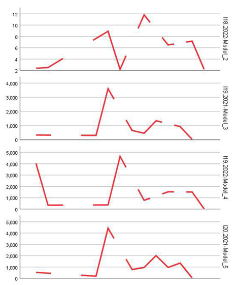
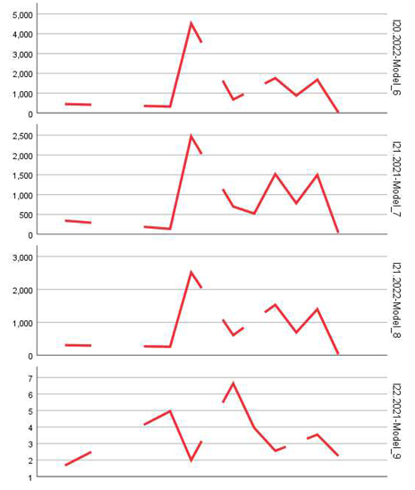
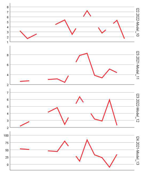
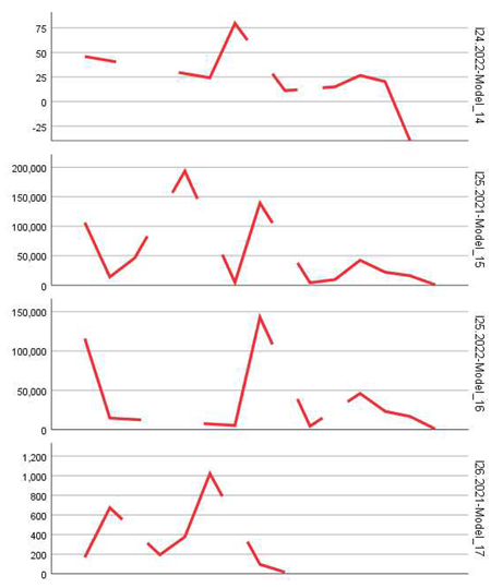
The main objective of this research was to evaluate entrepreneurial and labor market dynamics through a longitudinal analysis of 28 relevant statistical indicators from Eurostat, with projections toward 2035, in the post-pandemic context. The selected indicators reflect key aspects such as business creation and closure, survival rates, employment dynamics, the size and structure of the employed population in enterprises, as well as other indirect measures of economic resilience (tables and figures).

Countries: France, Romania, Slovenia, Germany, Croatia, Czech Republic, Sweden, Slovakia, Greece, Austria, Italy, Spain, Portugal, Bulgaria, Poland – \[https://doi.org/10.5281/zenodo.14713867].

2.2. Data Source and Indicator Selection

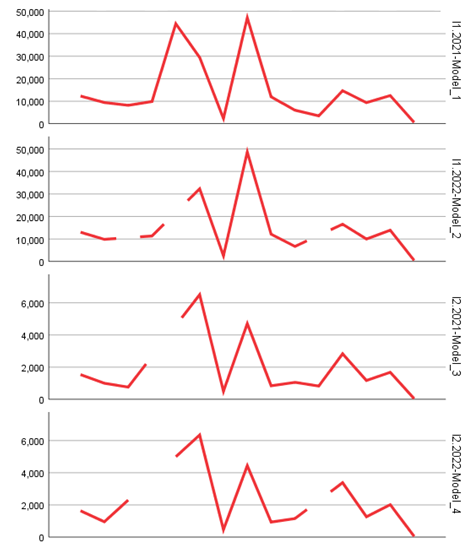
The data used came from official statistical sources, complemented by aggregations and transformations for modeling purposes. A total of 28 indicators (I1–I28) were analyzed, grouped into four main categories:

- Entrepreneurial demography (I1–I9)

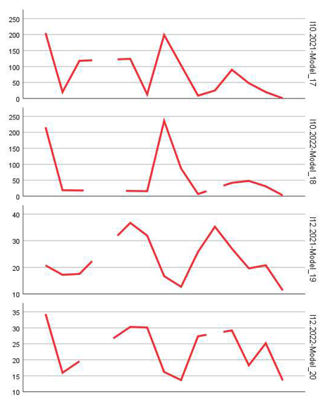
- Performance and growth (I10–I15)

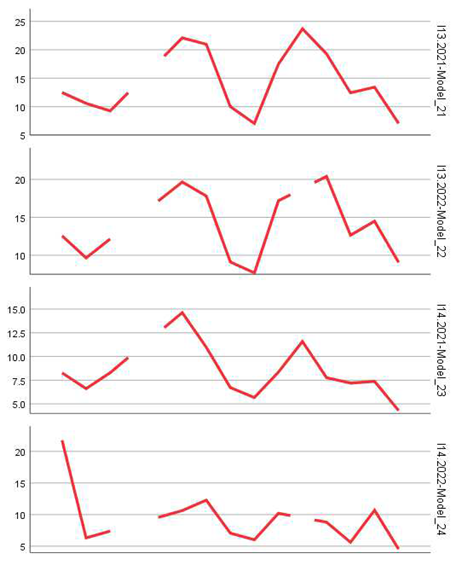
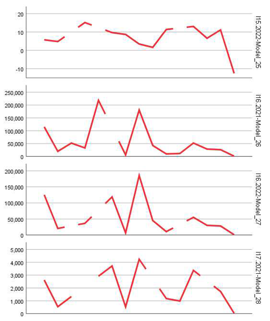
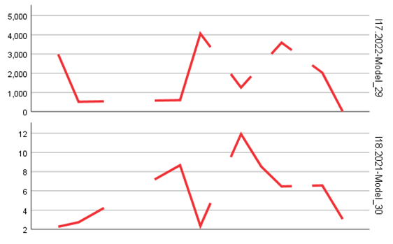
- Occupation and employment (I16–I24)

- Labor structure and distribution (I25–I28)

These indicators were calculated for each year, 2021 and 2022, resulting in 56 univariate time series, each analyzed using time series statistical modeling techniques.

2.3. Statistical Modeling Techniques

Two distinct modeling methods were applied to each time series:

- ARIMA models (Autoregressive Integrated Moving Average) – used for estimating and forecasting series with linear or autoregressive structure.

- Exponential smoothing models – used to capture trends and levels in the series, particularly for data without clear seasonality.

Modeling was done individually for each indicator, for both 2021 and 2022. Each model was automatically calibrated by selecting optimal parameters based on the Bayesian Information Criterion (BIC) and validated using statistical significance coefficients (p-values), standard error, and t-statistic values.

2.4. Model Fit Measures

To assess the quality of each estimated model, the following performance indicators were used:

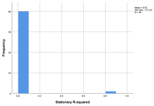
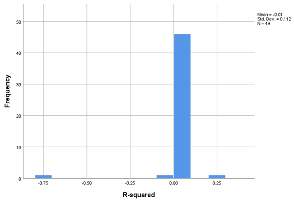
- R-squared and Stationary R-squared: indicate the proportion of total variance explained by the model.

- RMSE (Root Mean Squared Error): expresses the average deviation of estimated values from observed ones.

- MAPE (Mean Absolute Percentage Error) and MaxAPE: reflect relative errors, useful for comparing indicators on different scales.

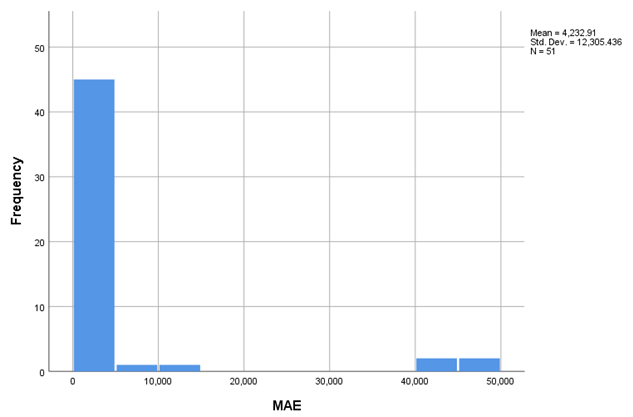
- MAE (Mean Absolute Error) and MaxAE: provide information on absolute deviations.

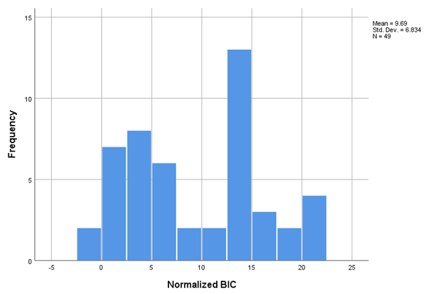
- Normalized BIC: penalizes model complexity to select the best-fitting model.

The overall average R-squared for the estimated models was -0.009, and the average Stationary R-squared was 0.018, suggesting a modest explanatory power of the models within the context of aggregated data. However, high values of RMSE and MaxAE for some indicators (e.g., I16, I25 – employees) are explained by the large numerical magnitude of these series.

2.5. Parameter Estimation and Statistical Significance

ARIMA models were applied with automatic parameter estimation to identify the autoregressive (p), differencing (d), and moving average (q) components. For example:

- For indicators I1 (number of enterprises) and I2 (enterprise births), the ARIMA models yielded significant coefficients (p < 0.01), indicating a strong autoregressive component.

- For indicators I3 and I8, the models identified direct and significant relationships between current and past values, with high t-statistic values (e.g., t = 9.244 for I3.2021).

- Certain indicators (e.g., I6.2021) did not produce significant coefficients, which may suggest either a lack of autocorrelation or high random variation.

Exponential smoothing models were applied only to indicators whose series showed no seasonality or autocorrelation. For instance, in model I14.2022, the parameter value α = 0.001 with a p-value > 0.99 indicates the absence of a significant trend. This aspect was considered in interpreting the results.

2.6. Methodological Limitations

Univariate modeling faces several limitations, including:

- Short time series – only two data points (2021, 2022) for each indicator may limit the relevance of dynamic models.

- Skewed data distributions, as evidenced by extreme values of skewness and kurtosis, which affect the robustness of estimates.

- Large estimation errors for indicators with high magnitudes (e.g., I16, I25), where large absolute variability affects the validity of direct comparisons.

Moreover, model performance was not consistent across indicators. For instance, I3, I8, and I12 showed high R-squared values and low errors, while I6 and I24 had lower predictive power.

2.7. Integrated Evaluation Approach

To overcome the limitations of individual models, the methodology included a comparative evaluation of model performance for each indicator in each year. This approach allowed for the identification of robust trends and relevant indicators for longitudinal analysis despite the uncertainties of the short time series.

Furthermore, the statistical significance of coefficients (t > 2 and p < 0.05) was used as a key criterion in interpreting indicator relevance in the results and discussion sections.

All models, except 24 – Holt and 40 – Simple, were ARIMA.

3. Results

3.1. General Evaluation of Model Performance

To assess the quality of the forecasting models applied to indicators related to business dynamics, several model fit indicators were analyzed, including the stationary and global R-squared, RMSE (Root Mean Square Error), MAE (Mean Absolute Error), MAPE (Mean Absolute Percentage Error), BIC (Bayesian Information Criterion), among others (tables and figures).

The overall performance of the ARIMA models was generally moderate, with an average R-squared value of -0.009, indicating a low capacity to explain the variation for most of the time series analyzed. However, this result should be interpreted in the context of high time series variability and the fact that univariate models did not include external explanatory variables. Even so, there were individual models with very strong performance, such as the one applied to indicator I14.2022 (stationary R-squared = 0.855), indicating a high explanatory power regarding the trend in the business mortality rate.

The average RMSE was approximately 5636.64, with a significant standard deviation (±16282.56), suggesting high variability in model performance. Very high RMSE values for certain indicators (e.g., I16 and I25, with values over 40,000) are due to the large absolute magnitude of these indicators (e.g., total number of employees or salaried persons).

The average MAPE was 384.43, indicating relatively high percentage errors overall, although for some series (e.g., I3, I8, I23), the errors were significantly lower. Likewise, the very high MaxAPE values, sometimes exceeding 10,000%, point to the presence of outliers or abrupt changes not efficiently captured by the models used.

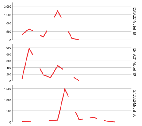
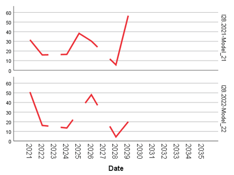
3.2. Results by Indicator

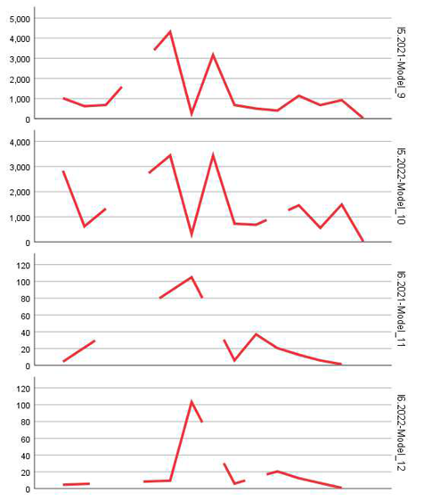
a. Structural and business dynamics indicators (i1–i5)

ARIMA models applied to the number of enterprises (I1) and birth/mortality indicators (I2 and I5) showed high statistical significance (p < 0.01), with large coefficients (e.g., 14,780.8 for I1.2021 and 1,417.18 for I5.2022). However, the R-squared values for these models remained near zero or negative (e.g., -0.723 for I6.2021), indicating a limited ability to capture temporal variation—likely due to nonlinear seasonality or structural shifts in the data.

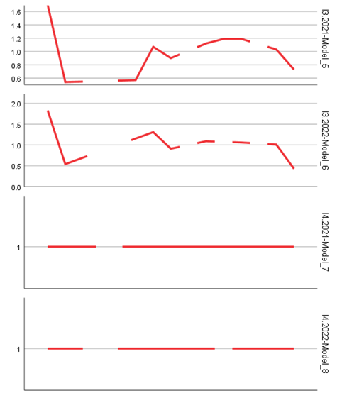
b. Survival and growth indicators (I6–I10)

Models associated with survival indicators (I6–I8) performed well in terms of coefficient significance, especially for I8 (p < 0.001 in both periods). The low error values (MAE under 2 for I8) suggest effective modeling of the share of surviving firms in the total population of active businesses. Additionally, models applied to I10 (high-growth enterprises) yielded statistically significant values and moderate errors (RMSE under 100).

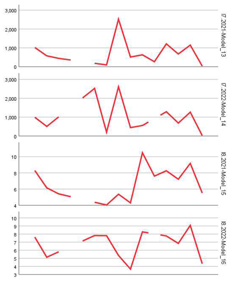
c. Percentage and occupational structure indicators (I18–I24)

For percentage-based indicators such as the employment rate in newly born enterprises (I18), business mortality rate (I14), or the employment growth rate in surviving firms (I24), the models achieved acceptable performance. The ARIMA model applied to I14.2022 stood out with a high R-squared value (0.855) and strong coefficient significance (p < 0.001), indicating a robust prediction of business mortality trends. Similarly, the model for I23.2022 (share of employment in surviving firms) showed high significance (t = 6.26, p < 0.001) and an extremely low absolute error (MAE = 1.46), underlining the robustness of the estimates.

d. Low-performance models

Some models displayed weak performance, especially where coefficients were not statistically significant (p > 0.1), such as I6.2021 (non-significant coefficient, p = 0.916) or I26.2022 (p = 0.122). These results may be due to irregular variation in the respective indicators or insufficient historical data for accurately modeling trends.

3.3. Parameters of the Exponential Smoothing Models

For a few indicators (e.g., I14.2022 and I23.2021), exponential smoothing model parameters were estimated. However, the estimated values for the alpha and gamma coefficients were extremely low or close to zero (alpha = 0.001 for I14.2022, alpha ≈ 0 for I23.2021), and the t-values did not show statistical significance (p > 0.99). This suggests that the simple exponential smoothing model failed to effectively capture the dynamics of the data and was inferior to the ARIMA model in this context.

Overall, the results indicate that although ARIMA models did not provide a strong general explanation for all analyzed series (with low average R-squared values), they still successfully captured statistically significant temporal relationships for many key indicators, especially those related to firm size, employment, and birth/mortality rates. The best-performing indicators were: I14 (mortality rate), I23 (share of employment in surviving firms), and I3/I8 (size and share of new enterprises).

Clearly, to improve the overall performance of the models, future research could benefit from the inclusion of relevant exogenous variables (e.g., macroeconomic factors, public policies supporting SMEs), as well as from multivariate approaches or machine learning models that can more effectively capture seasonality and nonlinear patterns in the data.

4. Discussion and Interpretations

4.1. Evaluation of Prediction Quality in the Socio-Economic Context

The results obtained from ARIMA and Exponential Smoothing models provide a detailed picture of their ability to capture the dynamics of indicators related to the structure and evolution of the entrepreneurial sector. Although the global R-squared coefficient was generally low, many models produced statistically significant coefficients, suggesting that these models have acceptable predictive value for an important subset of indicators (tables and figures).

In particular, models associated with the firm mortality rate (I14), the average size of newly established enterprises (I3), and the share of surviving firms (I8 and I23) provided robust estimates, consistent with the specialized literature. Thus, indicators expressing stable percentage structures or ratios between relative sizes appear more predictable than absolute indicators (e.g., number of employed persons – I16, I25), where extreme values and high variability limit prediction accuracy.

4.2. Sensitivity of Models to Indicator Type

Performance differences between models can be explained by the nature of the variables:

- Absolute indicators (e.g., I1, I16, I25) are harder to predict due to macroeconomic fluctuations, public policies, and other contextual factors. For example, for I16 (total number of employed persons), the RMSE was in the tens of thousands, and MaxAE exceeded 160,000, reflecting significant instability.

- Relative and percentage indicators (I3, I8, I14, I23) demonstrated greater structural stability and, consequently, better model performance. This suggests that simple autoregressive models are better suited to capturing percentage trends than raw volumes.

An interesting observation concerns the Exponential Smoothing models, which, although useful in predicting time series with linear trends or mild seasonality, proved inadequate for most indicators included in the analysis. For example, in the model for I14.2022, the alpha coefficient (0.001) and the extremely low t-statistic (t = 0.006, p = 0.995) indicate a lack of sensitivity to series variations. This underperformance suggests that the complex variability of the data requires more sophisticated methods than simple exponential smoothing.

4.3. Interpretation of Estimated Coefficients

The value and significance of ARIMA coefficients also provide a basis for economic interpretation:

- For indicator I1 (number of enterprises), the significant coefficient above 14,700 indicates a robust growth trend, possibly influenced by support measures for SMEs or post-pandemic economic recovery.

- For employment indicators in newly established firms (I17) and disappeared firms (I19), large and statistically significant coefficients reflect pronounced labor market volatility in the entrepreneurial sector.

- Additionally, positive and significant coefficients in models for I8 (share of surviving newborn firms) and I13 (birth rate) indicate relative resilience of Romanian entrepreneurship, with increased adaptability in the current economic context.

4.4. Model Limitations and Methodological Considerations

Although ARIMA models proved effective in capturing some trends, important limitations must be mentioned:

- Temporal collinearity and the absence of exogenous variables can lead to over- or underestimation of trends.

- Unexpected exogenous events (e.g., economic crises, legislative changes) are not captured by these models, reducing the relevance of long-term predictions.

- The models assumed stationarity of the time series, and in the absence of explicit stationarity tests (e.g., ADF or KPSS), this may introduce errors in model structuring.

4.5. Practical Implications and Future Directions

From a practical standpoint, the results can support policymakers and entrepreneurial ecosystem actors in:

- Identifying key indicators that provide early signals of structural changes (e.g., variations in I14 – firm mortality).

- Monitoring the effectiveness of public policies, especially through survival (I7, I8) and growth (I10, I24) indicators.

- Allocating resources and formulating targeted support strategies for newly established and vulnerable firms.

To improve model accuracy and robustness, the use of multivariate models (VAR, VECM) or neural network and machine learning approaches is advisable, as they can better capture nonlinear relationships and irregular seasonality. Additionally, integrating macroeconomic explanatory factors (e.g., inflation, GDP, unemployment) could significantly enhance the predictive power of the models.

5. Conclusions

The research demonstrated that ARIMA models can provide valuable insights for forecasting economic and entrepreneurial indicators, especially for percentage indicators or relative structures, such as the business mortality rate (I14) and the share of surviving firms (I23). These variables have a relatively stable structure, which allows for easier and more accurate modeling of economic dynamics. However, the ARIMA models showed modest performance for absolute indicators, such as the number of employees or the total volume of firms, due to large economic fluctuations and the external effects not included in the models. These prediction errors suggest that simple models are not sufficient to capture the complexity of the post-pandemic economic reality and labor market. Additionally, exponential smoothing models provided weak results, indicating that more sophisticated approaches, such as multivariate models or machine learning techniques, are needed to accurately capture variations in more complex economic data. In the future, integrating exogenous variables, such as macroeconomic factors or public policies, could significantly improve the accuracy and robustness of predictions. The study’s conclusions suggest that, to better understand long-term trends in entrepreneurship and the labor market, future research should adopt a more comprehensive approach, including global economic factors and advanced data analysis technologies. In this context, machine learning models, such as neural networks, could replace traditional techniques and provide more precise and relevant predictions. Additionally, comparative analysis between different countries could provide further insights into the specificities of post-pandemic economies and the measures that can support the sustainable development of small and medium-sized enterprises.

During the preparation of this manuscript, the authors utilized artificial intelligence tools for assistance in statistical analysis and data interpretation. Following this, the authors rigorously reviewed, validated, and refined all results, ensuring accuracy and coherence. The final content reflects the authors’ independent analysis, critical revisions, and scholarly judgment. The authors assume full responsibility for the integrity and originality of the published work.

Model Fit
Fit Statistic	Mean	SE	Minimum	Maximum	Percentile
					5	10	25	50	75	90	95
Stationary R-squared	0.018	0.122	-6.439	0.855	-6.661	-2.220	0.000	0.000	3.331	2.331	0.011
R-squared	-0.009	0.112	-0.723	0.282	-0.003	-6.661	0.000	0.000	3.331	1.887	3.608
RMSE	5636.637	16282.562	0.000	67159.532	0.206	1.701	3.703	71.032	1333.904	14057.805	59510.993
MAPE	384.434	467.783	0.000	2163.650	14.729	27.919	40.372	262.111	581.441	864.568	1595.239
MaxAPE	2730.751	3229.822	0.000	12170.833	41.692	74.518	103.027	2040.336	4478.512	7340.589	9945.458
MAE	4232.911	12305.436	0.000	49017.306	0.153	1.354	2.982	59.929	1012.198	9942.614	45652.542
MaxAE	12645.444	36912.004	0.000	161343.714	0.418	2.697	6.354	129.923	2647.625	33564.440	135525.617
Normalized BIC	9.687	6.834	-1.907	22.418	-0.037	1.370	3.299	9.129	14.722	19.309	22.211

Model Statistics.
Model	Model Fit statistics
I1.2021-Model_1	0.000	0.000	10213.413	19.309
I1.2022-Model_2	1.110	1.110	8859.417	19.199
I2.2021-Model_3	-2.220	-2.220	1328.769	15.244
I2.2022-Model_4	0.000	0.000	1454.959	15.330
I3.2021-Model_5	2.331	2.331	0.255	-1.907
I3.2022-Model_6	1.665	1.665	0.300	-1.395
I4.2021-Model_7			0.000
I4.2022-Model_8			0.000
I5.2021-Model_9	0.000	0.000	813.479	14.421
I5.2022-Model_10	0.000	0.000	1012.198	14.484
I6.2021-Model_11	-2.220	-0.723	12.782	6.151
I6.2022-Model_12	2.220	2.220	20.683	7.307
I7.2021-Model_13	2.220	2.220	476.278	13.227
I7.2022-Model_14	0.000	0.000	663.256	13.745
I8.2021-Model_15	1.887	1.887	1.692	1.606
I8.2022-Model_16	-6.661	-6.661	1.511	1.370
I10.2021-Model_17	0.000	0.000	59.929	8.724
I10.2022-Model_18	0.000	0.000	65.500	9.129
I12.2021-Model_19	-6.439	-6.439	6.759	4.405
I12.2022-Model_20	2.220	2.220	6.885	4.293
I13.2021-Model_21	5.551	5.551	4.933	3.701
I13.2022-Model_22	-4.441	-4.441	3.864	3.252
I14.2021-Model_23	4.774	4.774	1.906	2.197
I14.2022-Model_24	0.855	0.282	2.982	3.346
I15.2022-Model_25	-2.220	-2.220	4.953	4.166
I16.2021-Model_26	2.220	2.220	49017.306	22.418
I16.2022-Model_27	0.000	0.000	43925.125	22.121
I17.2021-Model_28	2.220	2.220	1271.960	14.844
I17.2022-Model_29	0.000	0.000	1284.375	14.919
I18.2021-Model_30	5.551	5.551	2.876	2.722
I18.2022-Model_31	4.441	4.441	3.144	2.878
I19.2021-Model_32	0.000	0.000	757.563	14.347
I19.2022-Model_33	0.000	0.000	1344.813	15.198
I20.2021-Model_34	1.110	1.110	899.481	14.636
I20.2022-Model_35	0.000	0.000	1022.125	14.807
I21.2021-Model_36	0.000	0.000	626.519	13.599
I21.2022-Model_37	-2.220	-2.220	671.156	13.714
I22.2021-Model_38	2.442	2.442	1.328	1.322
I22.2022-Model_39	7.772	7.772	1.701	1.682
I23.2021-Model_40	0.023	-0.007	1.622	1.785
I23.2022-Model_41	3.331	3.331	1.462	1.323
I24.2021-Model_42	1.110	1.110	23.205	7.072
I24.2022-Model_43	1.110	1.110	21.226	7.291
I25.2021-Model_44	3.331	3.331	48243.667	22.301
I25.2022-Model_45	0.000	0.000	40342.667	21.973
I26.2021-Model_46	0.000	0.000	279.837	12.060
I26.2022-Model_47	0.000	0.000	466.111	13.240
I27.2021-Model_48	3.331	3.331	281.222	12.129
I27.2022-Model_49	0.000	0.000	342.327	12.835
I28.2021-Model_50	0.000	0.000	12.996	5.940
I28.2022-Model_51	-6.661	-6.661	15.972	6.218

Model		Estimate	SE	t	Sig.
I14.2022-Model_24	Alpha (Level)	0.001	0.157	0.006	0.995
	Gamma (Trend)	1.000	200.050	0.005	0.996
I23.2021-Model_40	Alpha (Level)	2.348	0.287	8.196	1.000

ARIMA Model Parameters
		Estimate	SE	t	Sig.
I1.2021-Model_1	I1.2021	14780.800	3678.344	4.018	0.001
I1.2022-Model_2	I1.2022	14802.500	3840.639	3.854	0.003
I2.2021-Model_3	I2.2021	1803.000	513.320	3.512	0.004
I2.2022-Model_4	I2.2022	2056.909	576.636	3.567	0.005
I3.2021-Model_5	I3.2021	1.004	0.109	9.244	0.000
I3.2022-Model_6	I3.2022	1.023	0.155	6.617	0.000
I4.2021-Model_7	I4.2021	1.000	0.000
I4.2022-Model_8	I4.2022	1.000	0.000
I5.2021-Model_9	I5.2021	1107.462	340.115	3.256	0.007
I5.2022-Model_10	I5.2022	1417.182	377.696	3.752	0.004
I6.2021-Model_11	I6.2021	-0.926	8.245	-0.112	0.916
		1
I6.2022-Model_12	I6.2022	20.494	11.990	1.709	0.131
I7.2021-Model_13	I7.2021	761.583	193.963	3.926	0.002
I7.2022-Model_14	I7.2022	1007.273	261.008	3.859	0.003
I8.2021-Model_15	I8.2021	6.813	0.581	11.725	0.000
I8.2022-Model_16	I8.2022	6.695	0.536	12.479	0.000
I10.2021-Model_17	I10.2021	75.077	19.701	3.811	0.002
I10.2022-Model_18	I10.2022	70.500	27.064	2.605	0.029
I12.2021-Model_19	I12.2021	22.579	2.274	9.929	0.000
I12.2022-Model_20	I12.2022	23.107	2.313	9.989	0.000
I13.2021-Model_21	I13.2021	14.293	1.599	8.938	0.000
I13.2022-Model_22	I13.2022	13.662	1.375	9.939	0.000
I14.2021-Model_23	I14.2021	8.288	0.754	10.994	0.000
I15.2022-Model_25	I15.2022	6.535	2.090	3.127	0.010
I16.2021-Model_26	I16.2021	56947.286	17949.140	3.173	0.007
I16.2022-Model_27	I16.2022	55328.417	16558.387	3.341	0.007
I17.2021-Model_28	I17.2021	1892.300	471.384	4.014	0.003
I17.2022-Model_29	I17.2022	1882.375	539.182	3.491	0.010
I18.2021-Model_30	I18.2021	5.838	1.150	5.074	0.001
I18.2022-Model_31	I18.2022	5.456	1.309	4.167	0.004
I19.2021-Model_32	I19.2021	955.375	404.880	2.360	0.050
I19.2022-Model_33	I19.2022	1649.375	619.696	2.662	0.032
I20.2021-Model_34	I20.2021	1249.778	444.635	2.811	0.023
I20.2022-Model_35	I20.2022	1288.500	509.773	2.528	0.039
I21.2021-Model_36	I21.2021	887.556	264.743	3.353	0.010
I21.2022-Model_37	I21.2022	919.125	295.117	3.114	0.017
I22.2021-Model_38	I22.2021	3.445	0.601	5.729	0.001
I22.2022-Model_39	I22.2022	3.713	0.720	5.157	0.001
I23.2022-Model_41	I23.2022	3.768	0.602	6.263	0.000
I24.2021-Model_42	I24.2021	39.132	10.126	3.864	0.005
I24.2022-Model_43	I24.2022	22.806	11.891	1.918	0.097
I25.2021-Model_44	I25.2021	49918.333	18110.782	2.756	0.019
I25.2022-Model_45	I25.2022	41031.333	17427.494	2.354	0.046
I26.2021-Model_46	I26.2021	363.857	136.767	2.660	0.038
I26.2022-Model_47	I26.2022	490.833	263.686	1.861	0.122
I27.2021-Model_48	I27.2021	295.667	151.323	1.954	0.108
I27.2022-Model_49	I27.2022	274.857	201.406	1.365	0.221
I28.2021-Model_50	I28.2021	27.839	6.410	4.343	0.005
I28.2022-Model_51	I28.2022	25.467	7.874	3.234	0.023

References

- Adamides, E., & Karacapilidis, N. (2020). Information technology for supporting the development and maintenance of open innovation capabilities. Journal of Innovation & Knowledge, 5(1), 29–38. [CrossRef]
- Awschalom, D., Berggren, K. K., Bernien, H., Bhave, S., Carr, L. D., Davids, P., ... & Zhang, Z. (2021). Development of quantum interconnects (quics) for next-generation information technologies. PRX Quantum, 2(1), 017002. [CrossRef]
- Carayannis, E. G., & Morawska-Jancelewicz, J. (2022). The futures of Europe: Society 5.0 and Industry 5.0 as driving forces of future universities. Journal of the Knowledge Economy, 13(4), 3445–3471. [CrossRef]
- Chowdhury, M. Z., Shahjalal, M., Ahmed, S., & Jang, Y. M. (2020). 6G wireless communication systems: Applications, requirements, technologies, challenges, and research directions. IEEE Open Journal of the Communications Society, 1, 957–975. [CrossRef]
- Demirkan, S., Demirkan, I., & McKee, A. (2020). Blockchain technology in the future of business cyber security and accounting. Journal of Management Analytics, 7(2), 189–208. [CrossRef]
- Eurostat. (2025). Business demography and high growth enterprises by NACE Rev. 2 activity and other typologies \urt\_bd\_hgn\_\_custom\_15325082.
- Ghazal, T. M., Hasan, M. K., Alshurideh, M. T., Alzoubi, H. M., Ahmad, M., Akbar, S. S., ... & Akour, I. A. (2021). IoT for smart cities: Machine learning approaches in smart healthcare—A review. Future Internet, 13(8), 218. [CrossRef]
- Groher, T., Heitkämper, K., & Umstätter, C. (2020). Digital technology adoption in livestock production with a special focus on ruminant farming. Animal, 14(11), 2404–2413. [CrossRef]
- Heidari, A., Navimipour, N. J., & Unal, M. (2022). Applications of ML/DL in the management of smart cities and societies based on new trends in information technologies: A systematic literature review. Sustainable Cities and Society, 85, 104089. [CrossRef]
- Khan, N., Ray, R. L., Sargani, G. R., Ihtisham, M., Khayyam, M., & Ismail, S. (2021). Current progress and future prospects of agriculture technology: Gateway to sustainable agriculture. Sustainability, 13(9), 4883. [CrossRef]
- Levin, N., Kyba, C. C., Zhang, Q., de Miguel, A. S., Román, M. O., Li, X., ... & Elvidge, C. D. (2020). Remote sensing of night lights: A review and an outlook for the future. Remote Sensing of Environment, 237, 111443. [CrossRef]
- Liu, G., Huang, Y., Li, N., Dong, J., Jin, J., Wang, Q., & Li, N. (2020). Vision, requirements and network architecture of 6G mobile network beyond 2030. China Communications, 17(9), 92–104. [CrossRef]
- Mondini, A. C., Guzzetti, F., Chang, K. T., Monserrat, O., Martha, T. R., & Manconi, A. (2021). Landslide failures detection and mapping using Synthetic Aperture Radar: Past, present and future. Earth-Science Reviews, 216, 103574. [CrossRef]
- Nordhaus, W. D. (2021). Are we approaching an economic singularity? Information technology and the future of economic growth. American Economic Journal: Macroeconomics, 13(1), 299–332. [CrossRef]
- Vrontis, D., Christofi, M., Pereira, V., Tarba, S., Makrides, A., & Trichina, E. (2023). Artificial intelligence, robotics, advanced technologies and human resource management: A systematic review. Artificial Intelligence and International HRM, 172–201. [CrossRef]
- Waldschmidt, C., Hasch, J., & Menzel, W. (2021). Automotive radar—From first efforts to future systems. IEEE Journal of Microwaves, 1(1), 135–148. [CrossRef]
- [https://doi.org/10.1109/JMW.2020.3034644].
- Wenhua, Z., Qamar, F., Abdali, T. A. N., Hassan, R., Jafri, S. T. A., & Nguyen, Q. N. (2023). Blockchain technology: Security issues, healthcare applications, challenges and future trends. Electronics, 12(3), 546. [CrossRef]
- Wilkin, C. L., & Chenhall, R. H. (2020). Information technology governance: Reflections on the past and future directions. Journal of Information Systems, 34(2), 257–292. [CrossRef]
- Xie, R., Tang, Q., Wang, Q., Liu, X., Yu, F. R., & Huang, T. (2020). Satellite-terrestrial integrated edge computing networks: Architecture, challenges, and open issues. IEEE Network, 34(3), 224–231. [CrossRef]
- Xu, Y., Gui, G., Gacanin, H., & Adachi, F. (2021). A survey on resource allocation for 5G heterogeneous networks: Current research, future trends, and challenges. IEEE Communications Surveys & Tutorials, 23(2), 668–695. [CrossRef]
Disclaimer/Publisher’s Note: The statements, opinions and data contained in all publications are solely those of the individual author(s) and contributor(s) and not of MDPI and/or the editor(s). MDPI and/or the editor(s) disclaim responsibility for any injury to people or property resulting from any ideas, methods, instructions or products referred to in the content. |
© 2025 by the authors. Licensee MDPI, Basel, Switzerland. This article is an open access article distributed under the terms and conditions of the Creative Commons Attribution (CC BY) license (http://creativecommons.org/licenses/by/4.0/).
Copyright: This open access article is published under a Creative Commons CC BY 4.0 license, which permit the free download, distribution, and reuse, provided that the author and preprint are cited in any reuse.