
Submitted:
31 May 2025
Posted:
02 June 2025
You are already at the latest version
Abstract
Interpreting complex clinical time series is vital for patient safety and care, as it is both essential for supporting accurate clinical assessment and fundamental to building clinician trust and promoting effective clinical action. In complex time series analysis, decomposing a signal into meaningful underlying components is often a crucial means for achieving interpretability. This process is known as time series disentanglement. While deep learning models excel in predictive performance in this domain, their inherent complexity poses a major challenge to interpretability. Furthermore, existing time series disentanglement methods, including traditional trend or seasonality decomposition techniques, struggle to adequately separate clinically crucial specific components: static patient characteristics, condition trend, and acute events. Thus, a key technical challenge remains: developing an interpretable method capable of effectively disentangling these specific components in complex clinical time series. To address this challenge, we propose CoTD-VAE, a novel variational autoencoder framework for interpretable component disentanglement. CoTD-VAE incorporates temporal constraints tailored to the properties of static, trend, and event components, such as leveraging a Trend Smoothness Loss to capture gradual changes and an Event Sparsity Loss to identify potential acute events. These designs help the model effectively decompose time series into dedicated latent representations. We evaluate CoTD-VAE on critical care (MIMIC-IV) and human activity recognition (UCI HAR) datasets. Results demonstrate successful component disentanglement and promising performance enhancement in downstream tasks. Ablation studies further confirm the crucial role of our proposed temporal constraints. CoTD-VAE offers a promising interpretable framework for analyzing complex time series in critical applications like healthcare.
Keywords:
interpretation
; temporal constraints
; variational autoencoder
; disentanglement
; clinical time series
1. Introduction
In recent years, deep learning algorithms have made big progress in the field of time series data analysis. This has given us more advanced tools for analyzing complicated and ever-changing medical time series data [1]. Some computer science models, like RNNs, CNNs, and Transformers, have shown that they can better understand healthcare data over time. They are better at finding patterns in the data that are difficult to predict and complicated [2,3,4]. Information about healthcare, such as electronic health records (EHRs) and data from medical devices, contains a lot of useful clinical information. Using deep learning models to analyze medical data is hard to interpret [5,6,7]. To improve how the model is understood, it is necessary to make the model more transparent and analyze the way medical time series data is generated.
In the study of time series data, researchers have looked into and suggested different VAE-based time series decoupling models. These models break down complex time series data into its different parts, like trends, seasonality, and random noise [8,9,10]. Medical data that shows changes over time is often caused by a mix of things. It’s not enough to look at trends and seasons separately. We need better ways to separate these features that are more meaningful for doctors and patients. As a new way of thinking about data, disentangled representation learning has been studied a lot by academics recently [11]. The variational autoencoder (VAE) is a representation learning model that is often used. It achieves decoupling by learning a low-dimensional representation of the data and imposing specific a priori distribution constraints on it [12].
To improve the accuracy of the separation of features in time series data, we propose a new model called constrained Temporal Disentangled Variational Autoencoder (CoTD-VAE). The goal of the model is to disentangle complex medical time series data into three clinically relevant latent factors: the static factor, which captures baseline characteristics that are inherent to the patient and do not change or change very slowly over time; the trend factor, which represents the smooth evolution of disease states over time; and the event factor, which captures clinically important and transient changes in health status.
This is different from our previous work, which did not take into account the changing nature of healthcare data. Temporal constraints include Trend Smoothness Loss and Event Sparsity Loss. Trend Smoothness Loss helps the model learn smoother and continuous trends by penalizing sudden changes in trend latent variables over time. Event Sparsity Loss, on the other hand, tells the model to identify unexpected event points that are sparse in time and deviate from the regular trend. It does this by imposing sparsity constraints (e.g., L1 paradigm) on the event latent variables.
From the perspective of model architecture, CoTD-VAE is built on a base time series disentangled VAE model (Figure 1). The encoder is responsible for mapping the input medical time series into three separate latent spaces, namely static, trend and event. The decoder reconstructs the original input sequences using the learned latent variables (Figure 2). We introduced the aforementioned trend smoothness regularization term and event sparsity regularization term in addition to the standard reconstruction loss and KL scatter in the optimization objective (loss function) of the model. These learned disentangled representations (static, trend, event) can be applied to downstream prediction tasks. We demonstrate the higher quality of the learned disentangled representations through comparison and ablation experiments, where CoTD-VAE outperforms other benchmark models in terms of prediction performance for downstream tasks.This paper makes the following contributions:
- We propose a novel disentangled variational autoencode called "CoTD-VAE". It can disentangle medical time series data into three parts: static, trend, and event.
- CoTD-VAE is given explicit temporal constraints, which are the loss of trend smoothness and the loss of event sparsity. These constraints improve the model’s ability to capture and distinguish dynamic changes in medical data at different timescales.
- We evaluated the proposed CoTD-VAE and its learned Disentangled representation by running an experiment on a real healthcare risk prediction task. The results of the experiment showed that the proposed CoTD-VAE and its learned Disentangled representation are valid and better than other models.
The rest of this paper is organized as follows: Section II will review related work on time series analysis, learning of disentangled representations, and VAE applications in healthcare. Section III will explain the specific structure, mathematical rules, and how to implement our proposed CoTD-VAE. Section IV will present the dataset, the ways to measure performance, the basic model, and the detailed way the experiments were set up. Section V talks about the results of the experiment. Section VI will summarize the full paper and talk about possible future research directions.
2. Related Work
In this section, we look at research that is related to our proposed disentangled variational autocoder for time series. We also explore healthcare time series analysis, disentangled representation learning, and the use of variational autocoders in time series modeling. We focus on the challenges that existing approaches face when dealing with complex healthcare data.
2.1. Medical Time Series Analysis
Medical time series data analysis is an active area of research in clinical research and practice.Some common statistical methods, like autoregressive integral sliding average models (ARIMA) [13] and Kalman filtering [14], have been used to study and predict medical data. However, traditional linear models often have problems with modern healthcare big data that has complex nonlinear patterns and long-term dependencies. In recent years, deep learning models have been making progress in medical time series analysis because they can automatically learn features. Recurrent neural networks (RNNs) and their variants, such as long short-term memory networks (LSTMs) and gated recurrent units (GRUs), are now common methods in healthcare time series prediction. They are able to effectively model temporal dynamics in sequence data [15]. Different architectures, such as GRUs, LSTMs, and their bi-directional and multilayered variants, as well as feature-specific networks and target replication strategies, have specific advantages in different scenarios. Convolutional Neural Networks (CNNs) have a lot of potential in the field of recognizing and classifying Electroencephalography (EEG) signals. This is expected to provide efficient solutions to practical problems in medical and brain-computer interface systems [16]. A new Transformer model called ETHOS uses a zero-sample learning approach to predict future health trajectories. It analyzes high-dimensional, heterogeneous, and intermittent health data, such as patient health timelines (PHTs) [17].The Transformer architecture was used to train a large amount of EHR data ahead of time. This was done to predict the risk of serious lung problems in patients with SARS-CoV-2. It worked better than traditional machine learning models [18]. These methods have been very successful in improving how well predictions can be made. However, not enough attention has been paid to how easy it is to understand the representations learned by the model. This is especially true when it comes to disentangled latent factors, which is one of the things this study looks at.
2.2. Disentangled Representation Learning
The goal of Disentangled Representation Learning (DRL) is to allow a model to learn to separate potentially independent factors in the data. This improves the interpretability, generalization, and controllability of the representation [11]. The Variational Auto-Encoder (VAE) is a popular method for learning data distribution through something called variational inference. This is used in a process called disentangled representation learning, or DRL. Researchers have proposed various methods to improve the Disentangled ability of VAE on complex datasets. For example, -VAE makes latent variables more independent by adding a penalty term, which improves disentanglement. However, a large value can make reconstruction quality worse [19].FactorVAE forces latent variables to be independent by minimizing the Total Correlation, which improves disentanglement even more [20]. DIP-VAE improves the Disentangled performance by matching the covariance matrix and prior distribution of latent variables, which is useful in situations that require strict mathematical guarantees [21]. JointVAE can disentangle both continuous and discrete latent variables, which is useful in situations that require handling different types of latent factors [22].RF-VAE improves the decoupling capability by introducing correlation indicator variables to identify important latent factors [23]. By designing the right model structure and loss function, we can encourage VAE to learn a disentangled latent representation [24]. In the medical field, a method called "disentangled representation learning" has been used to study medical images and genetic data. This method helps identify what causes diseases and what types of diseases they are [25,26,27,28].
2.3. Disentangled Representation Learning for Time Series Based on LSTM, Transformer and VAE
The application of disentangled representation learning in the field of time series data analysis has driven research on Disentangled Temporal Variational Self-Encoder (DTSE) for time series [29,30,31]. The goal of these models is to break down a complex time series signal into several independent parts with specific meanings, such as trend and seasonality [32,33]. To achieve this goal, these methods typically use a variational autoencoder (VAE) as the main framework and use recurrent neural networks (RNNs) such as LSTM and Transformer, as well as convolutional neural networks (CNNs) as the encoder and decoder to capture the dynamic properties of the time series [34,35]. In the medical field, a type of machine learning called a VAE has been used to study heart signals. This type of VAE is called a "disentangled VAE." It can learn to understand different parts of a heartbeat signal. It can also spot things that are not normal[36]. However, these VAE variants of the approach are not very good at separating these different properties of the underlying factors when dealing with data with multiple complexities and lack temporal constraints specific to the characteristics of medical data [37].
3. Methods
This section describes CoTD-VAE, which is designed to learn separate representations of complex time series data and apply them to classification [38]. We start by explaining the overall structure of the model. Then, we look at its different parts, such as the encoder structure, decoder design, time limits, and training strategies. CoTD-VAE is made up of three parallel encoders, a decoder, and classifier module. CoTD-VAE Disentangled time series features are divided into three different latent variables: static features (), trend features (), and event features ().Given a time series , where C is the number of feature channels and L is the length of the series, the three encoders of CoTD-VAE map it to three independent latent distributions:
where and denote the mean and standard deviation functions, respectively, and diag denotes the diagonal covariance matrix.
Encoder design. CoTD-VAE uses three different encoder designs, each focusing on different types of time series features [39,40]. The static feature encoder uses a Temporal Encoder (TEC) architecture and supports either RNN or CNN implementations. The RNN mode uses a bidirectional LSTM to capture global sequence information. The CNN mode uses a convolutional layer and average pooling to extract the overall features of the sequence. The encoder shows the fixed dimensional latent variables that represent the static characteristics of the whole sequence. The trend feature encoder uses a one-dimensional convolutional network structure, which contains multilayer convolution, batch normalization, and Dropout layers. The output of this structure is a sequence of latent variables that is the same length as the sequence. This means that the time dimension information is retained, and the structure is suitable for capturing long-term change trends. The Event Feature Encoder is similar to the Trend Encoder, but it uses a special process called "sparsity regularization" to capture patterns that emerge or last for a short time. All encoders output mean and log-variance . Latent variables are sampled from the posterior distribution by a reparameterization trick : [41], where ⊙ denotes element-level multiplication, a trick that allows gradients to be back-propagated through a stochastic sampling process for end-to-end training.
Decoder design. The decoder receives a combined representation of the three latent variables and reconstructs the original time series. The specific implementation includes expanding the static latent variables to the same dimension as the length of the sequence, splicing the expanded static latent variables with the trend latent variables and the event latent variables in the feature dimension, averaging along the sequence dimensions, and finally reconstructing the original sequence by a Temporal Decoder (TD), which also supports RNN or CNN implementations.
Temporal constraints. We introduce temporal constraints [42] to guide different latent variables to learn specific types of features. The trend smoothness loss encourages the trending latent variables to vary smoothly in the time dimension by computing their first- and second-order differences and imposing an L2 paradigm penalty:
where B is the batch size and D is the dimension of the trend latent variable. If the sequence length is sufficient, we also compute a second-order difference loss to penalize acceleration changes:
The final trend smoothness loss is:
Event sparsity loss encourages event latent variables to be sparse in time, using a composite loss function:
is the L1 regularization term, which encourages overall sparsity; is the contrast loss, which encourages large values in a few dimensions, with the rest being close to zero; and is the peak loss, which encourages peak activation.
Training Goal. The goal of CoTD-VAE is to find the best way to minimize the following loss function:
is the reconstruction loss, computed using the mean squared error (MSE). , and are the KL scatter losses for each of the three latent variables. These losses measure the difference between the posterior distributions and the standard normal prior. , and are the weighting parameters for the KL scatter losses. These are designed as learnable parameters in this implementation. and are weight parameters for the temporal constraints. These are also designed as learnable parameters. During the training process, we use numerical stabilization techniques, such as cropping the gradient and loss values, to ensure the stability and convergence of the training.
Disentanglement and classfication. CoTD-VAE is trained through a two-step process [43]. This process separates representation learning and downstream task prediction. In the first stage, the variational self-encoder part is trained to learn high-quality latent representations. The training objective is to minimize the reconstruction loss, the KL scatter loss, and the temporal constraints. The classification loss is not included. After finishing the training, the encoder can map time series data to three disentangled potential spaces. In the second stage, we freeze the trained encoder parameters and pass the time series data through the trained VAE encoder to obtain the distribution parameters of the three latent variables: static, trend, and event. The statistical features of the three hidden variables are then put together into a long vector. This is used as input to the random forest to train and test the random forest classifier.
Assessment methods. We use the mean square error and mean absolute error to assess the ability of the model to reconstruct the original time series, assess the degree of disentanglement and expressiveness of the latent variables through visualization and statistical analysis, and compute prediction accuracy, precision, recall and F1 score.
4. Experiments
In this subsection, we design experiments to understand the performance and potential limitations of CoTD-VAE. The experimental objectives are as follows: 1) Verify the effectiveness of disentangled representation learning. 2) Evaluate the importance of the temporal consistency constraint. 3) Explore the generalization ability of CoTD-VAE on cross-domain data. 4) Discuss the interpretability and clinical application value of the latent representation.
4.1. Datasets
We performed our comparison and ablation experiments on two datasets. The first dataset is the UCI Human Activity Recognition (HAR) dataset [44]. It is a widely used benchmark dataset in the field of human activity recognition. This data set includes information from 30 volunteers (ages 19 to 48) who used their smartphones to record sensor data while doing six everyday activities. The activities were: WALKING, WALKING_UPSTAIRS, WALKING_DOWNSTAIRS, SITTING, STANDING, and LAYING. UCI HAR contains a total of 10,299 samples, which we divide into a training set (7,352 samples, about 71%) and a test set (2,947 samples, about 29%). We also divide 20% of the data in the training set as a validation set for optimizing the hyper-parameters and implementing the early stopping strategy. Each data sample has nine signal channels. These channels include total acceleration (X, Y, and Z axes), body acceleration (X, Y, and Z axes), and body gyroscope signals (X, Y, and Z axes). Initially, the signals were processed by a filter that reduced noise. Then, they were divided into segments using a fixed-width sliding window (2.56 seconds, 128 samples) with 50% window overlap. To prepare the data, we use a sliding window strategy. This means that we divide the sensor timing data into sections of 128 points each. Each section is 2.56 seconds of data, and the sections are 50% the same as the sections in the window right before it. We apply the MinMaxScaler technique to normalize all the feature values to the interval [0, 1]. This technique eliminates the scale difference between different features. It does so to ensure the stability of model training.
The second dataset was based on multivariate time-series data from the MIMIC-IV clinical [45]. This database documents the hospitalization of patients in the intensive care unit (ICU). The dataset is organized by patients and includes their important health information and details about the treatment they received during their stay in the ICU. The data were created using a sliding window approach. This means that a time_step was generated at 1-hour intervals. These time steps started from the patient’s time of admission to the ICU. Each time step is the same as a 3-hour observation window. Each window shows the patient’s status during that time period. Each time step has the patient’s main physiological information, like their average heart rate and average systolic blood pressure. It also has their lab results, like their highest platelet count and highest D-dimer value. And it has info on any medical treatments they received, like if they got anticoagulant therapy, when they were in the hospital, and if they were diagnosed with a blood clot-related disease.The dataset that was obtained after using SQL to make a request contained 130,000 samples. All of the samples were separated into three sets: a training set, a test set, and a validation set. We used a tool called StandardScaler in the scikit-learn library to adjust each feature so that the mean was 0 and the standard deviation was 1. This made the features more comparable and prepared the data for training the model.
4.2. Baselines
We considered three perspectives of comparison when choosing the baselines: 1) We will compare different sequence modeling structures. 2) We will compare generative and discriminative models (AE and VAE). 3) A comparison of different strategies for learning disentangled representations (-VAE, CVAE vs. CoTD-VAE). Four baseline methods are finally selected for comparison experiments. All of these methods provide ways to encode data and use these representations as features for later classification tasks.
Long Short-Term Memory Autoencoder (LSTM-AE) [46,47,48]: LSTM-AE is a classical approach for processing sequence data. It uses a bi-directional LSTM as an encoder and a uni-directional LSTM as a decoder. The encoder takes the input sequence and maps it to a fixed dimensional potential vector. The decoder uses this vector to reconstruct the original sequence. The specific structure includes an input projection layer, a bidirectional LSTM encoder (hidden layer dimension 128, 2-layer structure), a bottleneck layer (LN+ReLU activation) and a decoder. The MSE loss function is used for reconstruction.
Transformer Autoencoder (Transformer-AE) [49,50]: The Transformer architecture, which is based on the self-attention mechanism, has been successful in recent years in tasks that involve understanding sequences. Our version of Transformer-AE includes a Transformer encoder and decoder module that uses positional encoding to improve its ability to understand the order of events. The model dimension is set to 64, there are four attention heads, it contains two layers of encoder and decoder layers, and the feedforward network dimension is 128. Once again, mean squared error (MSE) is used as the reconstruction loss.
Beta-Variable Autoencoder (-VAE) [18]:-VAE is a type of VAE that allows you to adjust the weights () to balance how well something is reconstructed with how much it is represented. We use CNN as the main structure, and the encoder has several convolutional layers (channel configuration [16, 32], kernel size 5, step size 2) and a batch normalization layer that converts the inputs to the mean and variance parameters of the hidden variables. The decoder uses transposed convolution to recover the original sequence. The loss function combines two things: the reconstruction error and the weighted KL scatter.
Conditional Variational Autoencoder (CVAE) [51,52]: CVAE introduces category information as a condition into the generation process and learns the conditional distribution of specific activity categories. The structure is similar to -VAE, but it introduces category embedding (dimension 8) in both the encoding and decoding processes. This allows the model to generate specific reconstructions and learn representations that are sensitive to specific conditions.
We applied systematic hyperparameter optimization to all baseline models. We used a grid search strategy to explore different combinations of key hyperparameters for each model. These included hidden layer dimensions and number of layers for LSTM, model dimensions and number of attention heads for Transformer, latent space dimensions and regularization strengths for the VAE variant, etc. We chose the configuration with the best performance on the validation set for complete training.
After the representation learning phase is complete, we train a multilayer perceptron (MLP) classifier on the frozen encoder. This allows us to evaluate the discriminative performance of the potential representation. The classifier contains two hidden layers (dimensions 128 and 64, respectively) and uses BatchNorm and Dropout(0.3) to improve generalization. Training uses cross-entropy loss and Adam optimizer (learning rate 5e-4), and an early stopping strategy prevents overfitting.
4.3. Ablation Experiments
We used a multivariate time series dataset based on the MIMIC-IV clinical database to evaluate the impact of the trend smoothness constraint and the event sparsity constraint within the model. We constructed two CoTD-VAE variants:
- No Smoothness: It would be beneficial to consider removing the loss of trend smoothing and testing the impact of the trend smoothing constraints on the model performance.
- No Sparsity: It might be worthwhile to explore removing the loss of event sparsity and testing the impact of the event sparsity constraints on the model performance. By comparing the performance difference between these variants and the full model, we can hopefully quantify the contribution of these two components to the overall performance and verify the validity of our proposed temporal constraints.
5. Results
5.1. Reconstruction Task
The Mean Squared Error (MSE) and Mean Absolute Error (MAE) are employed to evaluate the reconstruction performance, which reflects the model’s ability to capture the essential features of the data. The Mean Squared Error (MSE) is defined as follows:
MSE is calculated as the mean of the square of the differences between the original data and the data that has been reconstructed. Here, denotes the original data point, denotes the corresponding reconstructed data point, and n is the total number of samples. This metric is more sensitive to larger errors, which are made bigger by squaring. It helps to identify significant reconstruction distortions. In activity recognition, MSE captures the model’s ability to remember the details of an action and is more sensitive to large-magnitude action features. Mean Absolute Error (MAE) is defined as follows:
MAE calculates the mean absolute difference between the original and reconstructed data. It uses for the original data points, for the reconstructed data points, and n for the total number of samples. MAE is less sensitive to outliers and provides a more balanced picture of overall reconstruction quality compared to MSE. These two error metrics work well together to provide a thorough assessment of how well the reconstruction is done. MSE focuses on capturing important details, while MAE shows how accurate the reconstruction is overall.

Table 1.
Performance on the UCI dataset reconstruction task.
| Model | MSE () | MAE () |
|---|---|---|
| LSTM-AE | 3.311 | 3.837 |
| Transformer-AE | 0.438 | 1.589 |
| -VAE | 6.616 | 5.145 |
| CVAE | 5.776 | 4.852 |
| CoTD-VAE | 3.267 | 3.422 |
CoTD-VAE outperforms LSTM-AE, -VAE, and CVAE across both MSE and MAE metrics. An interesting observation from the result is that Transformer-AE exhibits significantly lower MSE and MAE values compared to other models. Overfitting is potentially suggested by this.Despite the notable low reconstruction error, its generalization ability was further assessed through downstream prediction tasks.
To qualitatively assess the reconstruction fidelity of the trained CoTD-VAE on the UCI HAR dataset and visually demonstrate its temporal feature capture capabilities, a reconstruction visualization analysis was conducted using two samples selected from each of the SITTING and STANDING test sets. Figure 3 presents the results where each subplot provides a direct comparison between the original signal (blue curve) and its corresponding reconstructed signal (red curve) generated by the trained CoTD-VAE. Across all nine channels, these reconstructed signals closely track the overall trends and local fluctuations of the original signals, successfully capturing key features like the timing of peaks and troughs as well as approximate amplitude variations despite subtle discrepancies. Furthermore, the reconstruction results demonstrate high consistency across the different channels, indicating that the CoTD-VAE effectively learned the intrinsic data representation and is capable of accurately decoding it back into the original data space.
5.2. Classification Task
Accuracy, macro-averaged precision, macro-averaged recall and macro-averaged F1 score are used to evaluate the classification performance of the model. Accuracy is defined as follows:
The accuracy rate shows the proportion of activities that were correctly identified. is the number of true instances in category i, is the number of false positive instances in category i, and k is the total number of categories. In activity recognition, high accuracy means that the model can reliably tell the difference between different types of activities. Macro average precision, macro average recall and macro average F1 score are defined as follows:
Precision measures the reliability of the model to categorize samples into a particular class, where and denote the number of true and false-positive cases in class i, respectively. Recall measures the model’s ability to recognize all samples in a given category, where denotes the number of false negative cases in category i. The macro-averaging approach considers all activity categories equally and is not affected by category imbalance. The F1 score is a reconciled average of precision and recall, where and denote the precision and recall of category i, respectively.
Table 2 presents a comprehensive comparison of the overall classification performance across all evaluated models. Notably, CoTD-VAE outperformed all baseline methods on all classification metrics reported in Table 2, demonstrating its robust capability on classification task.
Table 3 lists the F1 Score, Precision, and Recall for different models across each activity category. Variations in performance between models and activity categories can be observed. CoTD-VAE consistently shows strong performance, ranking in the top two in most activity categories. CVAE performs exceptionally well in SITTING and STANDING, but shows significant weaknesses in other categories such as WALKING DOWNSTAIRS. LSTM-AE also performs prominently in LAYING and WALKING DOWNSTAIRS. LAYING appear to be easier for most models to predict, achieving very high or perfect metric scores.
5.3. Ablation Study
As shown in Table 4, removing either the trend smoothness loss or the event sparsity loss leads to a decrease in the model’s performance on the classification task. Removing the trend smoothness loss resulted in a 3.62 percentage point decrease in accuracy, a 5.04 percentage point decrease in F1 score, and a 0.6 percentage point decrease in AUC. Removing the event sparsity loss resulted in a 4.59 percentage point decrease in accuracy, a 6.04 percentage point decrease in F1 score, and a 1.3 percentage point decrease in AUC.
These results indicate that both temporal consistency constraints we introduced contribute to improving the model’s performance, with the event sparsity constraint contributing more significantly.
6. Discussion
The results of our experiment show that our proposed CoTD-VAE performed better than the baselines. The model can effectively separate static features, long-term trends, and sudden events in human activity data. Furthermore, by adding constraints based on time, the model’s ability to capture how things change over time was improved even more.
CoTD-VAE is better than other VAE versions (like BetaVAE and CVAE) at classifying data while still being good at making copies of the data. This shows that the disentangled latent representations and temporal consistency constraints are important for capturing the essential characteristics of activity data.
The study showed that the model performs better when the trends are smooth and there are fewer events. Visualization analysis of the hidden representations also showed that the hidden variables learned by the model can be understood and can reflect the characteristics of different activity classes and the relationships between them.
However, our study also has some limitations. For example, we only used two sets of data to evaluate the model. We need to use more diverse data in the future to see how well the model can generalize. It is important to note that our model still has room for improvement in distinguishing between the two activities, SITTING and STANDING.
7. Conclusions
CoTD-VAE effectively improves the model’s performance on reconstruction and classification tasks by disentangling time series data into latent factors such as static features, long-term trends, and abrupt events, and by introducing temporal consistency constraints such as trend smoothness and event sparsity. The CoTD-VAE’s disentanglement mechanism enables the model to extract different types of information from the time series. This meaningful decomposition enhances the model’s interpretability, allowing us to gain insight into the contribution of different latent factors to classification and providing more valuable features for downstream tasks. This is expected to significantly improve the accuracy and clinical utility of classification in medical time series data. Future work can explore the following directions:
- Further optimization of model architecture:Exploring more advanced sequence modeling architectures (e.g., more complex attention mechanisms) or different disentanglement methods to further enhance the separability and expressiveness of latent representations. Also, investigating how to adaptively determine the dimensions of each latent space and the weights of the regularization terms (e.g., the and parameters) instead of using fixed hyperparameter settings.
- More fine-grained latent factor analysis and clinical association: Conducting more in-depth analysis of the disentangled static, trend, and event latent spaces, for example, by using clustering, visualization, or other statistical methods, to identify clinically meaningful subgroups or patterns. Further collaborate with domain experts to validate the clinical interpretability of these latent factors and their association strength with specific disease states or risk events.
- Application to wider medical time series tasks: Applying the CoTD-VAE model to other types of medical time series data (e.g., physiological waveforms, continuous glucose monitoring data, etc.), as well as different clinical tasks, such as early disease diagnosis, disease progression prediction, treatment response assessment, or patient phenotyping.
- Enhancing model generalization ability and transferability: Investigating how to improve the generalization ability of trained models across different hospitals or patient populations. Exploring federated learning or transfer learning techniques in order to utilize data from multiple sources while protecting data privacy, aiming to train more robust models.
- Integration with causal inference: Exploring the combination of disentangled representations with causal inference methods to better understand the causal relationships between different latent factors and how they jointly influence patient risk outcomes. This will help reveal the underlying disease mechanisms and provide guidance for clinical interventions.
These future research directions will further advance the development of medical time series analysis and risk prediction techniques based on deep generative models and disentangled representation learning.
Author Contributions
Conceptualization, L.H.; methodology, L.H. and Q.C.; software, L.H.; validation, L.H.; formal analysis, L.H.; investigation, L.H.; resources, Q.C.; data curation, L.H.; writing—original draft preparation, L.H.; writing—review and editing, Q.C.; visualization, L.H.; supervision, Q.C.; project administration, Q.C.. All authors have read and agreed to the published version of the manuscript.
Funding
This research received no external funding.
Institutional Review Board Statement
Not applicable.
Informed Consent Statement
Not applicable.
Data Availability Statement
Not applicable.
Conflicts of Interest
The authors have no competing interests to declare that are relevant to the content of this article.
References
- Sakib, M.; Mustajab, S.; Alam, M. Ensemble deep learning techniques for time series analysis: a comprehensive review, applications, open issues, challenges, and future directions. Cluster Computing 2025, 28, 1–44. [Google Scholar] [CrossRef]
- Kumaragurubaran, T.; Senthil Pandi, S.; Vijay Raj, S.R.; Vigneshwaran, R. Real-time Patient Response Forecasting in ICU: A Robust Model Driven by LSTM and Advanced Data Processing Approaches. 2024 2nd International Conference on Networking and Communications (ICNWC) 2024, 1–6. [Google Scholar]
- Aminorroaya, A.; Dhingra, L.; Zhou, X.; Camargos, A.P.; Khera, R. A NOVEL SENTENCE TRANSFORMER NATURAL LANGUAGE PROCESSING APPROACH FOR PRAGMATIC EVALUATION OF MEDICATION COSTS IN PATIENTS WITH TYPE 2 DIABETES IN ELECTRONIC HEALTH RECORDS. Journal of the American College of Cardiology 2025, 85, 407–407. [Google Scholar] [CrossRef]
- Patil, S.A.; Paithane, A.N. Advanced stress detection with optimized feature selection and hybrid neural networks. International Journal of Electrical and Computer Engineering (IJECE) 2025, 15, 1647–1655. [Google Scholar] [CrossRef]
- Xie, F.; Yuan, H.; Ning, Y.; Ong, M.E.H.; Feng, M.; Hsu, W.; Chakraborty, B.; Liu, N. Deep learning for temporal data representation in electronic health records: A systematic review of challenges and methodologies. Journal of biomedical informatics 2022, 126, 103980. [Google Scholar] [CrossRef]
- Lan, W.; Liao, H.; Chen, Q.; Zhu, L.; Pan, Y.; Chen, Y.-P. DeepKEGG: a multi-omics data integration framework with biological insights for cancer recurrence prediction and biomarker discovery. Briefings in Bioinformatics 2024, 25. [Google Scholar] [CrossRef] [PubMed]
- Li, S.; Chen, Q.; Liu, Z.; Pan, S.; Zhang, S. Bi-SGTAR: A simple yet efficient model for circRNA-disease association prediction based on known association pair only. Knowledge-Based Systems 2024, 291, 111622. [Google Scholar] [CrossRef]
- Li, Y.; Lu, X.; Wang, Y.; Dou, D. Generative time series forecasting with diffusion, denoise, and disentanglement. Advances in Neural Information Processing Systems 2022, 35, 23009–23022. [Google Scholar]
- Neloy, A.A.; Turgeon, M. A comprehensive study of auto-encoders for anomaly detection: Efficiency and trade-offs. Machine Learning with Applications 2024, 100572. [Google Scholar] [CrossRef]
- Asesh, A. Variational Autoencoder Frameworks in Generative AI Model. In ; IEEE, 2023; pp. 01–06. In Proceedings of the 2023 24th International Arab Conference on Information Technology (ACIT); IEEE, 2023; pp. 01–06. [Google Scholar]
- Wang, X.; Chen, H.; Tang, S.; Wu, Z.; Zhu, W. Disentangled representation learning. IEEE Transactions on Pattern Analysis and Machine Intelligence 2024. [Google Scholar] [CrossRef]
- Liang, S.; Pan, Z.; Liu, W.; Yin, J.; De Rijke, M. A survey on variational autoencoders in recommender systems. ACM Computing Surveys 2024, 56, 1–40. [Google Scholar] [CrossRef]
- Box, G.E.P.; Jenkins, G.M.; Reinsel, G.C.; Ljung, G.M. Time Series Analysis: Forecasting and Control; John Wiley & Sons, Inc.: Hoboken, New Jersey, 2015. [Google Scholar]
- Shakandli, M.M. State Space Models in Medical Time Series. Ph.D. Thesis, University of Sheffield, 2018. [Google Scholar]
- Morid, M.A.; Sheng, O.R.L.; Dunbar, J. Time series prediction using deep learning methods in healthcare. ACM Transactions on Management Information Systems 2023, 14, 1–29. [Google Scholar] [CrossRef]
- Rajwal, S.; Aggarwal, S. Convolutional neural network-based EEG signal analysis: A systematic review. Archives of Computational Methods in Engineering 2023, 30, 3585–3615. [Google Scholar] [CrossRef]
- Renc, P.; Jia, Y.; Samir, A.E.; Was, J.; Li, Q.; Bates, D.W.; Sitek, A. Zero shot health trajectory prediction using transformer. NPJ Digital Medicine 2024, 7, 256. [Google Scholar] [CrossRef]
- Lentzen, M.; Linden, T.; Veeranki, S.; Madan, S.; Kramer, D.; Leodolter, W.; Fröhlich, H. A transformer-based model trained on large scale claims data for prediction of severe COVID-19 disease progression. IEEE Journal of Biomedical and Health Informatics 2023, 27, 4548–4558. [Google Scholar] [CrossRef] [PubMed]
- Higgins, I.; Matthey, L.; Pal, A.; Burgess, C.P.; Glorot, X.; Botvinick, M.M.; Mohamed, S.; Lerchner, A. beta-VAE: Learning Basic Visual Concepts with a Constrained Variational Framework. In International Conference on Learning Representations; 2016.
- Kim, H.; Mnih, A. Disentangling by Factorising. In International Conference on Machine Learning; 2018.
- Kumar, A.; Sattigeri, P.; Balakrishnan, A. Variational inference of disentangled latent concepts from unlabeled observations. arXiv, 2017; arXiv:1711.00848 2017. [Google Scholar]
- Dupont, E. Learning disentangled joint continuous and discrete representations. Advances in neural information processing systems 2018, 31. [Google Scholar]
- Kim, M.; Wang, Y.; Sahu, P.; Pavlovic, V. Relevance factor vae: Learning and identifying disentangled factors. arXiv, 2019; arXiv:1902.01568 2019. [Google Scholar]
- Liu, Z.; Li, M.; Han, C.; Tang, S.; Guo, T. STDNet: Rethinking disentanglement learning with information theory. IEEE Transactions on Neural Networks and Learning Systems 2023. [Google Scholar] [CrossRef]
- Liu, X.; Sanchez, P.; Thermos, S.; O’Neil, A.Q.; Tsaftaris, S.A. Learning disentangled representations in the imaging domain. Medical Image Analysis 2022, 80, 102516. [Google Scholar] [CrossRef]
- Cheng, J.; Gao, M.; Liu, J.; Yue, H.; Kuang, H.; Liu, J.; Wang, J. Multimodal disentangled variational autoencoder with game theoretic interpretability for glioma grading. IEEE Journal of Biomedical and Health Informatics 2021, 26, 673–684. [Google Scholar] [CrossRef]
- Yu, H.; Welch, J.D. MichiGAN: sampling from disentangled representations of single-cell data using generative adversarial networks. Genome biology 2021, 22, 158. [Google Scholar] [CrossRef]
- Qiu, Y.L.; Zheng, H.; Gevaert, O. Genomic data imputation with variational auto-encoders. GigaScience 2020, 9, giaa082. [Google Scholar] [CrossRef] [PubMed]
- Lim, M.H.; Cho, Y.M.; Kim, S. Multi-task disentangled autoencoder for time-series data in glucose dynamics. IEEE Journal of Biomedical and Health Informatics 2022, 26, 4702–4713. [Google Scholar] [CrossRef] [PubMed]
- Hahn, T.V.; Mechefske, C.K. Self-supervised learning for tool wear monitoring with a disentangled-variational-autoencoder. International Journal of Hydromechatronics 2021, 4, 69–98. [Google Scholar] [CrossRef]
- Wu, S.; Haque, K.I.; Yumak, Z. ProbTalk3D: Non-Deterministic Emotion Controllable Speech-Driven 3D Facial Animation Synthesis Using VQ-VAE. In Motion in Games; 2024. [Google Scholar]
- Wang, Z.; Xu, X.; Zhang, W.; Trajcevski, G.; Zhong, T.; Zhou, F. Learning latent seasonal-trend representations for time series forecasting. Advances in Neural Information Processing Systems 2022, 35, 38775–38787. [Google Scholar]
- Liu, X.; Zhang, Q. Combining Seasonal and Trend Decomposition Using LOESS with a Gated Recurrent Unit for Climate Time Series Forecasting. IEEE Access 2024. [Google Scholar] [CrossRef]
- Staffini, A.; Svensson, T.; Chung, U.; Svensson, A.K. A disentangled VAE-BiLSTM model for heart rate anomaly detection. Bioengineering 2023, 10, 683. [Google Scholar] [CrossRef]
- Buch, R.; Grimm, S.; Korn, R.; Richert, I. Estimating the value-at-risk by Temporal VAE. Risks 2023, 11, 79. [Google Scholar] [CrossRef]
- Kapsecker, M.; Möller, M.C.; Jonas, S.M. Disentangled representational learning for anomaly detection in single-lead electrocardiogram signals using variational autoencoder. Computers in Biology and Medicine 2025, 184, 109422. [Google Scholar] [CrossRef]
- Li, Y.; Chen, Z.; Zha, D.; Du, M.; Ni, J.; Zhang, D.; Chen, H.; Hu, X. Towards learning disentangled representations for time series. In Proceedings of the 28th ACM SIGKDD Conference on Knowledge Discovery and Data Mining; 2022; pp. 3270–3278. [Google Scholar]
- Pinheiro Cinelli, L.; Araújo Marins, M.; Barros da Silva, E.A.; Lima Netto, S. Variational Autoencoder. In Variational Methods for Machine Learning with Applications to Deep Networks; Springer International Publishing: Cham, 2021; pp. 111–149. [Google Scholar]
- Fortuin, V.; Baranchuk, D.; Rätsch, G.; Mandt, S. Gp-vae: Deep probabilistic time series imputation. In International conference on artificial intelligence and statistics; PMLR, 2020; pp. 1651–1661.
- Hsu, W.-N.; Zhang, Y.; Glass, J. Unsupervised learning of disentangled and interpretable representations from sequential data. Advances in neural information processing systems 2017, 30. [Google Scholar]
- Rezende, D.J.; Mohamed, S.; Wierstra, D. Stochastic Backpropagation and Approximate Inference in Deep Generative Models. PMLR 2014, 32, 1278–1286. [Google Scholar]
- Zhao, Y.; Zhao, W.; Boney, R.; Kannala, J.; Pajarinen, J. Simplified temporal consistency reinforcement learning. In International Conference on Machine Learning; PMLR, 2023; pp. 42227–42246. [Google Scholar]
- Lan, W.; Li, C.; Chen, Q.; Yu, N.; Pan, Y.; Zheng, Y.; Chen, Y.-P. LGCDA: Predicting CircRNA-Disease Association Based on Fusion of Local and Global Features. IEEE/ACM Transactions on Computational Biology and Bioinformatics 2024, 21, 1413–1422. [Google Scholar] [CrossRef] [PubMed]
- Anguita, D.; Ghio, A.; Oneto, L.; Parra, X.; Reyes-Ortiz, J.L. Human activity recognition on smartphones using a multiclass hardware-friendly support vector machine. In Ambient Assisted Living and Home Care: 4th International Workshop, IWAAL 2012, Vitoria-Gasteiz, Spain, December 3-5, 2012. Proceedings 4; Springer, 2012; pp. 216–223. [Google Scholar]
- Johnson, A.E.W.; Bulgarelli, L.; Shen, L.; Gayles, A.; Shammout, A.; Horng, S.; Pollard, T.J.; Moody, B.; Gow, B.; Lehman, L.-w.H.; Celi, L.A.; Mark, R.G. MIMIC-IV, a freely accessible electronic health record dataset. Scientific Data 2023, 10. [Google Scholar] [CrossRef] [PubMed]
- Xie, F.; Xiao, F.; Tang, X.; Luo, Y.; Shen, H.; Shi, Z. Degradation State Assessment of IGBT Module Based on Interpretable LSTM-AE Modeling Under Changing Working Conditions. IEEE Journal of Emerging and Selected Topics in Power Electronics 2024, 12, 5544–5557. [Google Scholar] [CrossRef]
- Madhukar, S.R.; Singh, K.; Kanniyappan, S.P.; Krishnan, T.; Sarode, G.C.; Suganthi, D. Towards Efficient Energy Management of Smart Buildings: A LSTM-AE Based Model. In 2024 International Conference on Electronics, Computing, Communication and Control Technology (ICECCC); 2024; pp. 1–6.
- Han, Z.; Tian, H.; Han, X.; Wu, J.; Zhang, W.; Li, C.; Qiu, L.; Duan, X.; Tian, W. A Respiratory Motion Prediction Method Based on LSTM-AE with Attention Mechanism for Spine Surgery. Cyborg and Bionic Systems 2023, 5. [Google Scholar] [CrossRef]
- Prabhakar, C.; Li, H.; Yang, J.; Shit, S.; Wiestler, B.; Menze, B.H. ViT-AE++: Improving Vision Transformer Autoencoder for Self-supervised Medical Image Representations. In International Conference on Medical Imaging with Deep Learning; 2023.
- Vaswani, A.; Shazeer, N.M.; Parmar, N.; Uszkoreit, J.; Jones, L.; Gomez, A.N.; Kaiser, L.; Polosukhin, I. Attention is All you Need. In Neural Information Processing Systems; 2017.
- Sun, W.; Xiong, W.; Chen, H.; Chiplunkar, R.; Huang, B. A Novel CVAE-Based Sequential Monte Carlo Framework for Dynamic Soft Sensor Applications. IEEE Transactions on Industrial Informatics 2024, 20, 3789–3800. [Google Scholar] [CrossRef]
- Kim, J.; Kong, J.; Son, J. Conditional Variational Autoencoder with Adversarial Learning for End-to-End Text-to-Speech. ArXiv 2106. [Google Scholar]
Figure 1.
Basic Variational Autoencoder Model, consisting of an encoder and a decoder. The input data is analyzed by the encoder to produce means and variances, and reparameterization is used to obtain latent variables. These latent variables are fed into the decoder to reconstruct the original data, with the aim of minimizing the sum of reconstruction error and KL divergence to optimize reconstruction performance.
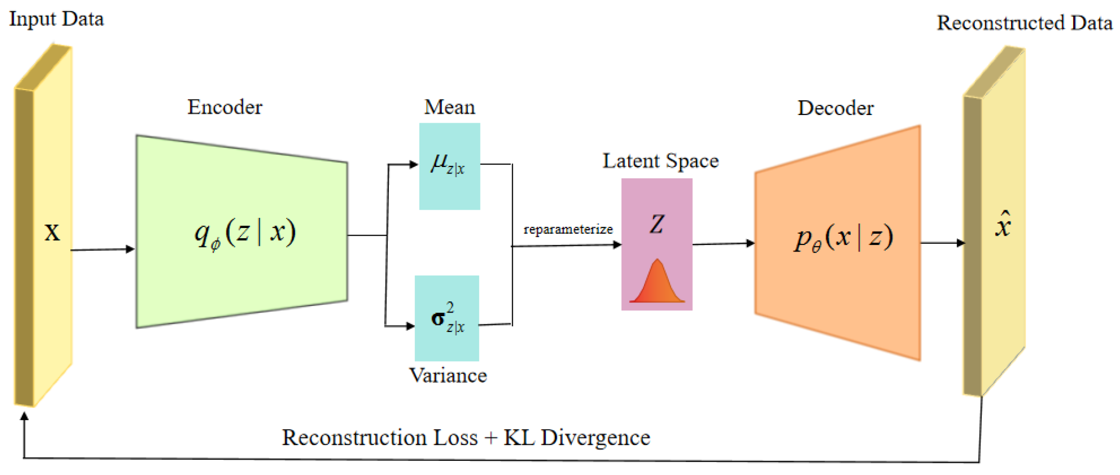
Figure 2.
CoTD-VAE is an advanced VAE model tailored for medical time series data. It uses three encoders to disentangled input data into latent variables , , and . During backpropagation optimization, it adds minimizing trend smoothness loss and event sparsity loss.
Figure 2.
CoTD-VAE is an advanced VAE model tailored for medical time series data. It uses three encoders to disentangled input data into latent variables , , and . During backpropagation optimization, it adds minimizing trend smoothness loss and event sparsity loss.
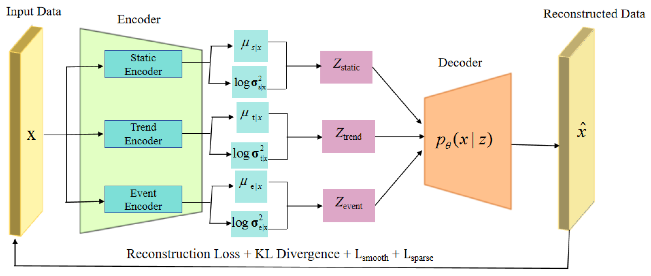
Figure 3.
Visualization of CoTD-VAE Signal Reconstruction on UCI HAR Dataset. Comparison of original signals (blue curves) and signals reconstructed by the CoTD-VAE model (red curves) for selected SITTING and STANDING activity samples from the test set. The visualization across nine sensor channels demonstrates the model’s high fidelity in capturing key temporal features and overall signal structure.
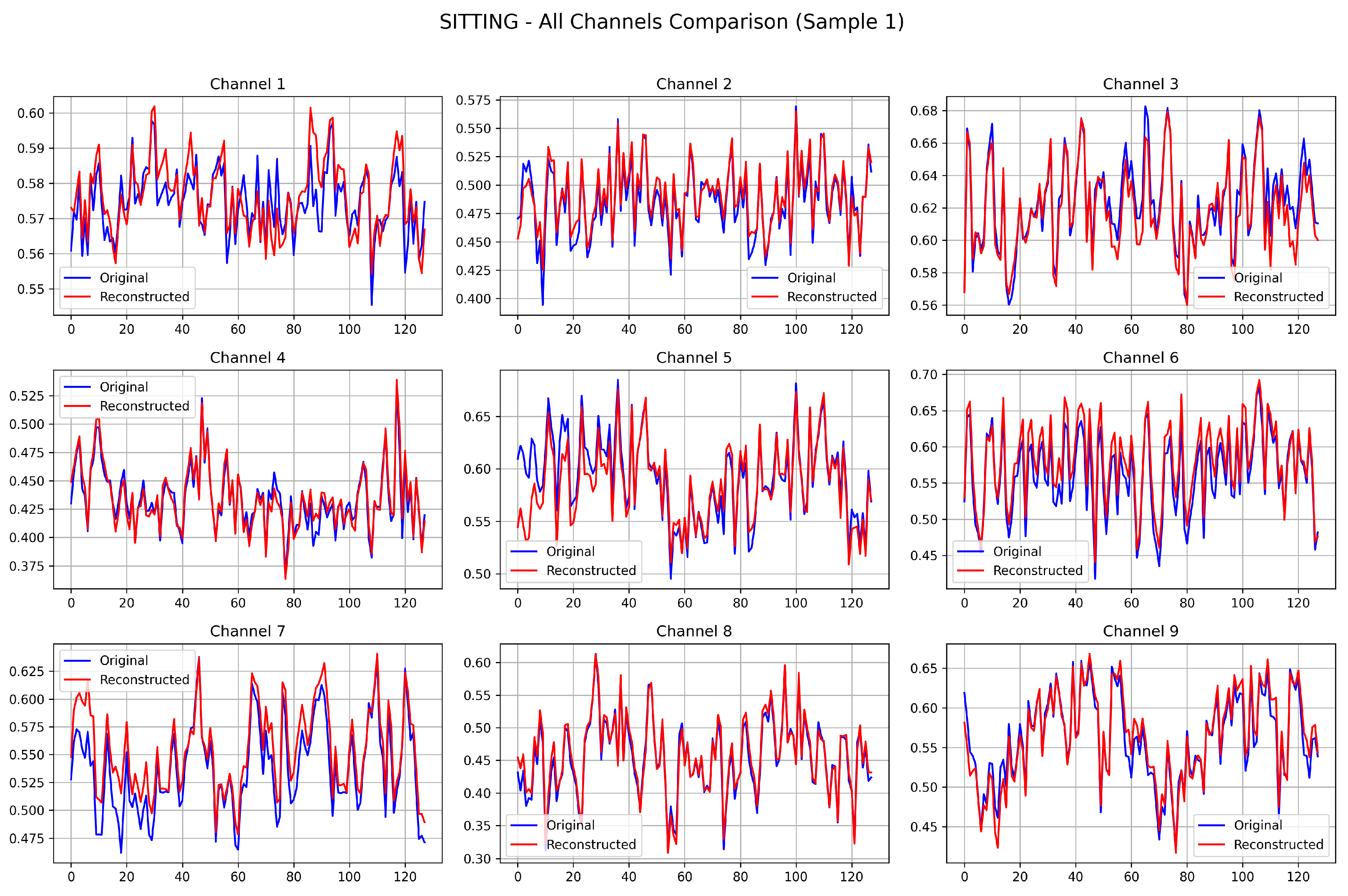
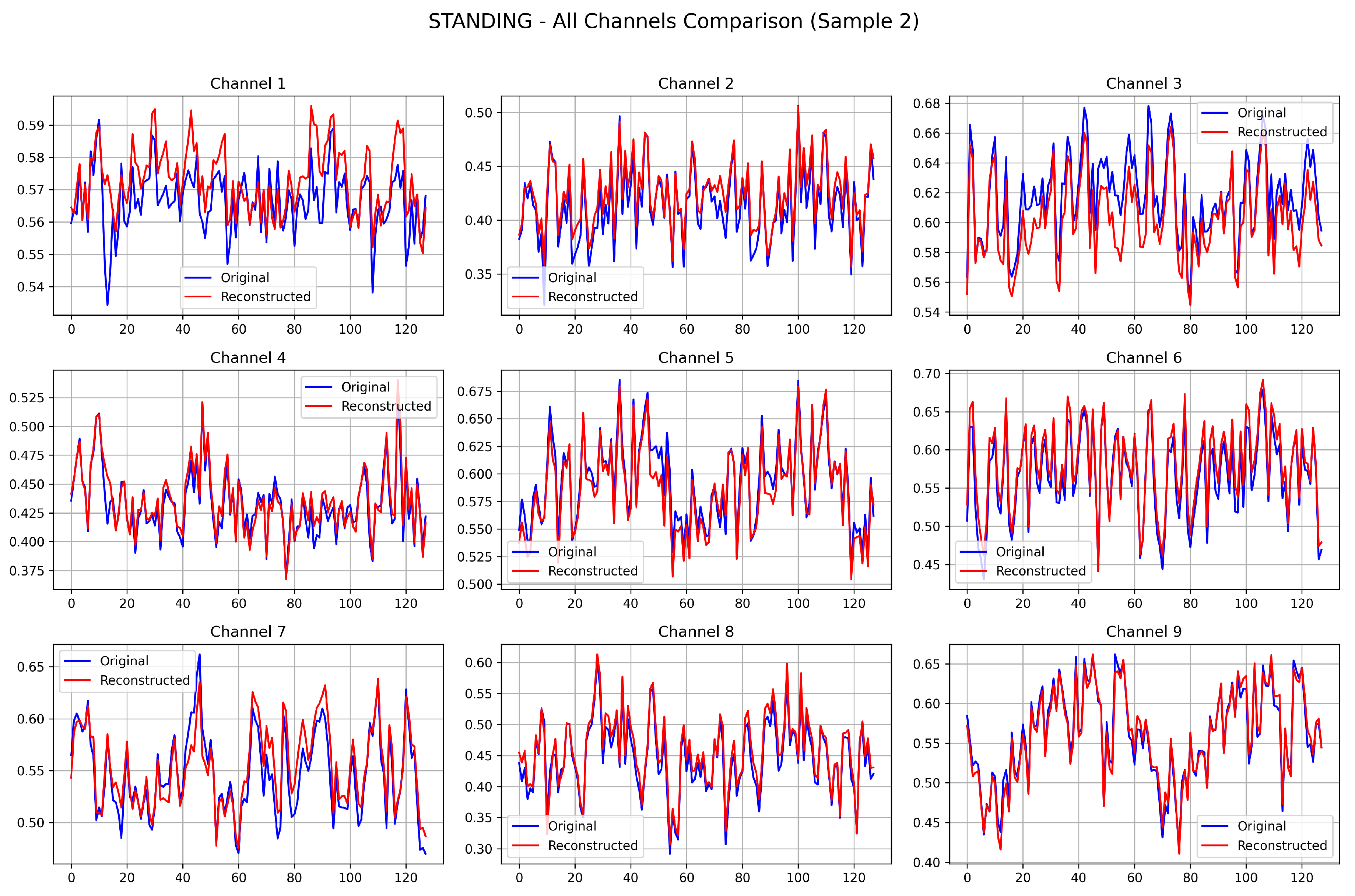
Table 2.
Aggregate performance of models on the classification task.
| Model | Accuracy | Macro-averaged F1 |
Macro-averaged Precision |
Macro-averaged Recall |
|---|---|---|---|---|
| LSTM-AE | 0.8850 | 0.8851 | 0.8888 | 0.8862 |
| Transformer-AE | 0.8599 | 0.8586 | 0.8582 | 0.8591 |
| -VAE | 0.8677 | 0.8661 | 0.8670 | 0.8666 |
| CVAE | 0.8717 | 0.8605 | 0.8627 | 0.8618 |
| CoTD-VAE | 0.9026 | 0.9027 | 0.9030 | 0.9027 |
Table 3.
F1 Score, Precision, and Recall for each activity category.
| Metric | Model | Walk | Walk Up | Walk Down | Sit | Stand | Lay |
|---|---|---|---|---|---|---|---|
| F1 Score | LSTM-AE | 0.893 | 0.881 | 0.947 | 0.782 | 0.807 | 1.000 |
| Transformer-AE | 0.831 | 0.836 | 0.882 | 0.791 | 0.813 | 0.999 | |
| -VAE | 0.909 | 0.845 | 0.849 | 0.794 | 0.826 | 0.973 | |
| CVAE | 0.759 | 0.811 | 0.684 | 0.984 | 0.942 | 0.983 | |
| CoTD-VAE | 0.901 | 0.865 | 0.962 | 0.832 | 0.857 | 1.000 | |
| Precision | LSTM-AE | 0.860 | 0.987 | 0.899 | 0.790 | 0.797 | 1.000 |
| Transformer-AE | 0.834 | 0.832 | 0.874 | 0.793 | 0.819 | 0.998 | |
| -VAE | 0.896 | 0.861 | 0.820 | 0.824 | 0.802 | 0.998 | |
| CVAE | 0.770 | 0.801 | 0.765 | 0.978 | 0.895 | 0.968 | |
| CoTD-VAE | 0.888 | 0.869 | 0.962 | 0.853 | 0.846 | 1.000 | |
| Recall | LSTM-AE | 0.929 | 0.796 | 1.000 | 0.774 | 0.818 | 1.000 |
| Transformer-AE | 0.829 | 0.841 | 0.890 | 0.788 | 0.806 | 1.000 | |
| -VAE | 0.921 | 0.830 | 0.881 | 0.766 | 0.852 | 0.950 | |
| CVAE | 0.748 | 0.822 | 0.619 | 0.990 | 0.994 | 0.998 | |
| CoTD-VAE | 0.913 | 0.860 | 0.962 | 0.813 | 0.868 | 1.000 |
**Activity abbreviations:** Walk (Walking), Walk Up (Walking Upstairs), Walk Down (Walking Downstairs), Sit (Sitting), Stand (Standing), Lay (Laying).
Table 4.
Ablation Study Results of the CoTD-VAE Model on Classification Task.
| Model | Accuracy | F1 Score | AUC |
|---|---|---|---|
| CoTD-VAE | 0.8707 | 0.6092 | 0.918 |
| No Smoothness | 0.8345 | 0.5588 | 0.912 |
| No Sparsity | 0.8248 | 0.5488 | 0.905 |
Disclaimer/Publisher’s Note: The statements, opinions and data contained in all publications are solely those of the individual author(s) and contributor(s) and not of MDPI and/or the editor(s). MDPI and/or the editor(s) disclaim responsibility for any injury to people or property resulting from any ideas, methods, instructions or products referred to in the content. |
© 2025 by the authors. Licensee MDPI, Basel, Switzerland. This article is an open access article distributed under the terms and conditions of the Creative Commons Attribution (CC BY) license (http://creativecommons.org/licenses/by/4.0/).
Copyright: This open access article is published under a Creative Commons CC BY 4.0 license, which permit the free download, distribution, and reuse, provided that the author and preprint are cited in any reuse.


