
Submitted:
30 May 2025
Posted:
31 May 2025
You are already at the latest version
Abstract
To monitor the quality of machine process, we proposed a method for debris counting in video sequences. In the method, we firstly present a novel framework called GM-YOLOv11-DNMS to track the debris, and then a video-level post-processing algorithm for debris counting in videos. The GM-YOLOv11-DNMS has two main improvements: (1) it replaces the CNN layers with Ghost Module in YOLOv11n, significantly reducing computational costs while maintaining detection performance, and (2) it uses a new Dynamic Non-Maximum Suppression (DNMS) method, which adjusts dynamically thresholds to improve detection accuracy. The post-processing method uses a trigger signal from rising edges to improve debris counting in the video streams. Experimental results show that The Ghost Module reduces FLOPs from 6.48G to 5.72G compared to YOLOv11n, with negligible accuracy loss, while the DNMS algorithm improves debris detection precision across different YOLO versions. The proposed framework achieves Precision, Recall, and mAP@0.5 values of 97.04%, 96.38% and 95.56%, respectively, in image-based detection tasks. In video-based experiments, the proposed video-level post-processing algorithm combined with GM-YOLOv11-DNMS achieves a crack-debris counting accuracy of 90.14%. This lightweight and efficient approach is particularly effective in detecting small-scale objects within images and accurately analyzing dynamic debris in video sequences, providing a robust solution for automated debris monitoring in machine tool processing applications.
Keywords:
ghost module
; YOLOv11
; DNMS
; debris
; video
1. Introduction
With the rise of dark factories, automated machining quality monitoring has become an essential requirement in modern manufacturing. To monitor the machining process, online measurements for various physical parameters has been widely used in factory. These parameters include torque, acceleration, temperature, acoustic emission, displacement, and cutting force, which are critical for ensuring process optimization and product quality [1,2]. Traditionally, experienced workers evaluated processing quality and machine tool status by examining the shape and number of debris. Recently, many studies have also explored the relationship between debris and processing quality. For example, Tao Chen et al. [3] tested the relationship between debris morphology and surface quality of product in their high-speed hard-cutting experiment with PCBN tools on hardened steel GCr15. They found that tools with variable chamfered edges produced more regular and stable debris. However, tools with uniform chamfered edges experienced a transition in debris morphology from wavy to irregular curves over time. Yaonan Cheng et al. [4] found that in the process of heavy milling of 508III steel, the debris morphology changes significantly at different stages of tool wear. Firstly, the debris are C-shaped at the beginning of wear stage, then the shape change to strip-like formations as wear intensifies and ultimately becoming spiral when the tool experiences severe wear. Research by Vorontsov [5] found that Band-type debris can scratch the workpiece surface or damage cutting edges, while C-shaped debris can affect surface roughness, and shattered debris tend to wear down the sliding surfaces of the machine tool. However, in practical, although the pixel quality and sampling rates of current cameras have already met the requirements for monitoring debris, automated monitoring of debris in factories to manage processing conditions is not commonly observed. This is because two key challenges must be addressed: first, how to perform target detection of debris, and second, how to count the number of debris particles appearing in the video.
With the development of deep learning algorithms, many excellent object detection algorithms have emerged, which may suitable for detect debris and processing the processing video [6]. Among these algorithms, YOLO (You Only Look Once) is one of the most prominent and widely applied in various fields, such as firefighting [7] , monitoring [8] , agricultural production [9] , and defect detection [10]. The early YOLOv1 significantly improved detection speed through its end-to-end single-stage detection framework, but its localization accuracy and adaptability to complex scenarios were relatively weak. Subsequent versions introduced optimizations from various perspectives. For instance, YOLOv3 [11] enhanced the detection capability for small objects by incorporating multi-scale prediction and residual structures. YOLOv4 [12] integrated self-attention mechanisms and Cross-Stage Partial Networks (CSPNet), which improved feature representation while maintaining real-time performance. YOLOv7 [13] proposed a scalable and efficient network architecture, utilizing reparameterization techniques to achieve parameter sharing. YOLOv8 [14] further optimized the training process by introducing a dynamic label assignment strategy, which enhanced convergence efficiency. YOLOv9 [15] addressed the limitations of information loss and deep supervision in deep learning by introducing Programmable Gradient Information (PGI) and a Generalized Efficient Layer Aggregation Network (Gelan). YOLOv10 [16] integrated global representation learning capabilities into the YOLO framework while maintaining low computational costs, significantly enhancing model performance and facilitating further improvements.
In addition to version updates, numerous scholars have made improvements to various iterations of YOLO. For instance, Doherty et al. [17] introduced the BiFPN (Bidirectional Feature Pyramid Network) into YOLOv5, enhancing its multi-scale feature fusion capabilities. Jianqi Yan et al. [18] incorporated the CBAM (Convolutional Block Attention Module) into YOLOv7 and YOLOv8, while Jinhai Wang et al. [19] integrated the SE (Squeeze-and-Excitation) module into YOLOv5, thereby improving the model's ability to focus on critical features. Furthermore, Mengxia Wang et al. proposed DIoU-NMS [20] based on YOLOv5, addressing the issue of missed detection in densely packed objects. These advancements collectively contribute to the refinement and robustness of the YOLO framework. Besides, the lightweight design of models has also garnered significant attention. For instance, Chen Xue et al. [21] proposed a Sparsely Connected Asymptotic Feature Pyramid Network, which optimized the architecture of YOLOv5 and YOLOv8. Yong Wang et al. [22] combined the PP-LCNet backbone network with YOLOv5, effectively reducing the model's parameter count and computational load. Among various lightweight strategies, the Ghost Module [23] has emerged as a notable technique, capable of generating the same number of feature maps as conventional convolutional layers but with significantly reduced computational costs. This module can be seamlessly integrated into YOLO networks to minimize computational overhead. Previous studies have demonstrated the applicability of the Ghost Module in versions such as YOLOv5 and YOLOv8, achieving a reduction in model parameters while maintaining detection accuracy [24,25]. However, to our knowledge, no research has yet explored the impact of integrating the Ghost Module into the more recent YOLOv11.Additionally, it is noteworthy that starting from version 10, YOLO introduced the dual label assignments and consistent matching metric strategy [19]. Benefiting from this strategy, we can choose to use the original one-to-many head for training and then perform inference using the Non-Maximum Suppression (NMS) algorithm, or use a one-to-one detection head to directly obtain the inference results (also referred to as NMS-free training). Although NMS-free training results in lower inference latency, according to the literature [19], it requires more one-to-one matching discriminative features and may reduce the resolution of feature extraction.
Therefore, in this paper, we introduce the Ghost Module into YOLOv11 and continue to employ the traditional one-to-many training approach. Also, we propose a novel Dynamic Non-Maximum Suppression (DNMS) algorithm to improve the accuracy of debris detection. Moreover, we present a post-processing methods for debris counting in dynamic video sequences. The main novelties and contributions of this paper can be summarized as below:
- Compared the performance of different YOLO versions in detecting debris in images of machining processes.
- Ghost module is introduced to backbone of the standard YOLO v11 to reduce the computation.
- Dynamic Non-Maximum Suppression algorithm is proposed to enhance the accuracy in identifying little objects, in this paper it’s debris.
- Based on the rising edge signal trigger mechanism, a video-level post-processing algorithm has been developed to automatically count the amount of debris that falls within the video.
The remainder of the paper is organized as follows: Section 2 summarizes the structure of GM-YOLOv11 and presents the Dynamic Non-Maximum Suppression algorithm and the video-level post-processing algorithm in detail. Analysis of the proposed algorithms and the experimental results are provided in Section 3. Other details related to the proposed algorithms are given in Section 4.Finally, Section 5 concludes this paper.
2. Materials and Methods
2.1. GM-YOLOv11
2.1.1. YOLOv11
YOLO (You Only Look Once) is a one-stage object detection algorithm. Its core idea is to model the object detection task as an end-to-end regression problem. It directly predicts the bounding boxes and class probabilities of all objects in an image through a single forward pass. Compared to algorithms like R-CNN, YOLO can leverage global contextual information and reduce computational resource usage.So it is suitable for real-time monitoring tasks. YOLOv11 introduces numerous improvements over its predecessors compared to the previous version. The key advantages of YOLOv11 can be included as: better feature extraction; optimized efficiency and speed; fewer parameters with higher accuracy; cross-environment adaptability; and support for a wide range of tasks. The architecture of YOLOv11n is shown as in Figure 1.
Detailed network structure and model parameter information of YOLOv11n used in this paper are shown as in Figure 1. YOLOv11n is consists of three critical components: Backbone, Neck, and Head. The backbone is responsible for extracting key features at different scales from the input image. This component consists of multiple convolutional blocks (Conv), each of which contains three sub-blocks, as illustrated in ‘b’ block of Figure 1: Conv2D, BatchNorm2D, and the SiLU activation function. In addition to Conv blocks, YOLOv11n also includes multiple C3K2 blocks, which replace the C2f blocks used in YOLOv8, optimizing CSP (Cross-Stage Partial) design, thereby reducing computational redundancy in YOLOv11n, as shown in ‘e’ block of Figure 1. The C3K2 blocks provide a more computationally efficient implementation of CSP. The final two modules in the Backbone are SPPF (Spatial Pyramid Pooling Fast) and C2PSA (Cross-Stage Partial with Spatial Attention). The SPPF module utilizes multiple max-pooling layers (as shown in Figure 1(f)) to efficiently extract multi-scale features from the input image. On the other hand, as depicted in ‘g’ block of Figure 1, the C2PSA module incorporates an attention mechanism to enhance the model’s accuracy.
The second major structure of YOLOv11n is the neck. The neck consists of multiple Conv layers, C3K2 blocks, Concat operations, and upsampling blocks, leveraging the advantages of the C2PSA mechanism. The primary function of the Neck is to aggregate features at different scales and pass them to the Head structure.
The final structure of YOLOv11n is the head, a crucial module responsible for generating prediction results. It determines object categories, calculates objectness scores, and accurately predicts the bounding boxes of identified objects.It is worth noting that YOLOv11n, being the smallest model in the YOLOv11 series, has only one detect layer, while the YOLOv11s, YOLOv11m, YOLOv11l, and YOLOv11x models all feature three detect layers.
From the structure of YOLOv11n, it is evident that YOLOv11n achieves efficient multi-scale feature extraction and fusion by optimizing the design of the backbone, neck, and head. Its structural highlights include the C3K2 blocks, SPPF module, and the C2PSA attention mechanism. Through a size-specific model pruning strategy, YOLOv11n significantly enhances resource efficiency while maintaining high accuracy. In this paper, YOLOv11n is used to extract not only debris but also workpiece. And the predicted location of workpiece will be used for improving the result for detecting debris.
2.1.2. Ghost Module
The Ghost Module is a model compression technique [23]. Compared to traditional convolutional modules, the Ghost Module reduces overall computational costs by controlling the number of filters in the first part of the standard convolution and generating additional feature maps using low-cost linear operations. This approach reduces the number of parameters and computational complexity without altering the size of the output feature maps. The Ghost Module consists of three steps: primary convolution, ghost generation, and feature map concatenation. The structure of the Ghost Module is illustrated in Figure 2.
Figure 2(a) illustrates the computational approach of a standard convolutional network. The relationship of input and output can be expressed as:
where * is the convolution operation, b is the bias term,c is the number of input channels and h and w are the height and width of the input data. is the spatial size of the output feature map.n is the number of filters. is the convolution filters in this layer. is the kernel size of convolution filters. Compared to the standard convolutional network, the Ghost Module reduces the number of required parameters and computational complexity . Its implementation contain a primary convolution process and a cheap operation process as illustrated in Figure 2(b). In the primary convolution, m (where ) intrinsic feature maps are generated, as formulated in Equation (2).
where is the utilized filters. As formulated in Equation (3), in the cheap operation, a series of cheap linear operations is applied on each intrinsic feature in to generate s ghost features.
where is the intrinsic feature map in , is the j-th linear operation. As specified in [23], the d×d linear convolution kernels of are required to maintain consistent dimensions for distinct indices i and j. s can be get by . By consolidating the terms in Equation (3), we derive the aggregated output tensor . This demonstrates that the standard convolution output and the ghost module output exhibit identical dimensionality. Consequently, the ghost module achieves plug-and-play compatibility, serving as a drop-in replacement for conventional convolutional layers. And the computational cost ratio and parameter ratio between standard convolution and ghost convolution are expressed by Equation (4) and (5), respectively:
As revealed in Equations (4) and (5), the parameter determines the degree of model compression: the tensor size of intrinsic feature maps is compressed to compared with that of standard convolution modules, since the magnitude of d and k are similar in size and .
From Equations (2) and (3), it can be observed that the ghost convolution incorporates two hyperparameters: the kernel size () and the number of ghost features generated from a single intrinsic feature map .
2.1.3. GM-YOLOv11
In both the backbone and head of YOLOv11, multiple convolutional layers are included. To reduce the computational load of YOLOv11, we replaced the convolutional layers in the backbone and head with Ghost Modules. We designed three models by replacing only the backbone, only the head, and replacing both entirely, named GM-YOLOv11-backbone, GM-YOLOv11-head, and GM-YOLOv11, respectively. The specific architectures are illustrated in Figure 3, Figure 4 and Figure 5.
The detailed network architectures and parameter configurations of GM-YOLOv11-backbone, GM-YOLOv11-head, and GM-YOLOv11 used in this study are illustrated in Appendix A.1,Appendix A.2 and Appendix A.3, respectively. By comparing Figs. 3, 4, and 5 with Fig. 2, it is evident that GM-YOLOv11-backbone integrates five ghost modules into the backbone of the standard YOLOv11n model, while GM-YOLOv11-head introduces four such modules, and GM-YOLOv11 incorporates nine. This modification results in an increase in the number of layers but a reduction in the total number of parameters. Specifically, the standard YOLOv11n comprises 319 layers, whereas GM-YOLOv11-backbone, GM-YOLOv11-head, and GM-YOLOv11 have 339, 327, and 347 layers, respectively. In terms of parameters, the standard YOLOv11n contains 2,590,230 parameters, while GM-YOLOv11-backbone, GM-YOLOv11-head, and GM-YOLOv11 are optimized to 2,354,294, 2,500,470, and 2,264,534 parameters, respectively. According to reference [23], the kernel size for the cheap operation is set to , and the mapping ratio for the ghost module is set to . Notably, the architectures of C3K, C3K2, bottleneck, Conv2d, SPPF, C2PSA, and PSA modules remain unchanged, as their effectiveness has been well-established in their respective roles. Maintaining these components ensures the preservation of the model's performance and stability, allowing us to focus on optimizing other aspects of the network. Furthermore, their proven efficiency contributes to achieving a desirable balance between accuracy and computational complexity.
2.2. Dynamic Non-Maximum Suppression Algorithm (DNMS)
It is worthy to see that starting from version 10, YOLO provides a non-NMS method.However, since debris does not occupy many pixels, this paper still adopts a one-to-many head for debris detection to maintain the resolution of feature extraction. Moreover,in this paper, YOLO are used to extract not only debris but also workpieces. The detected position of workpieces are used to develop DNMS. Our aims are statistic the debris appears in the video. Considering the when debris on the workpieces and away from the workpiece may different at shape and scale. We develop the DNMS to enhance the GM-YOLOv11 and help distinguish debris as leaving debris and left debris.
2.2.1. Leaving Debris and Left Debris
Observing the machining process of the workpiece, it can be seen that when debris is generated on the workpiece, it typically forms a continuous curl. This type of debris is referred to as "leaving debris." After the debris breaks away from the workpiece, it is influenced by the high-speed rotation of the workpiece and flies off in various directions, which we term as "left debris." The left debris may predominantly be curled, but some of it can also appear as small, fragmented, and complex-shaped particles. While the leaving debris overlaps with the workpiece, it is especially important to note that the debris shares the same material as the workpiece, resulting in consistent colors. Therefore, this study sets different non-maximum suppression thresholds based on whether the debris overlaps with the workpiece pixels, as shown in Figure 6b.
2.2.2. Box Size Adjustment
During the Non-Maximum Suppression (NMS) process, bounding boxes are suppressed by calculating IoU values between the Ground Truth and the predicted bounding boxes. The formula for the standard IoU computation is shown in Equation (6):
From Equation (6), it can be observed that the IoU value is related to both the area of the Ground Truth and the area of the predicted bounding box. However the debris are usually very small, as a result,When predicted bounding boxes deviate from their true positions, the NMS algorithm can easily lead to false positives or missed detections, especially in scenarios with overlapping objects or localization errors. In actual processing, in most images, there will be a leaving debris. When the debris is ejected, the most likely situation in the image is the presence of one leaving debris and one left debris. Since the breaking of debris is a random behavior, the possibility of multiple left debris appearing in images where debris have broken off is also very high. Based on this possibility, this paper first introduces a scaling mechanism the size of the predicted bounding box. Through this adjustment, the monitoring results can be better combined with actual conditions.
In this paper the size of predicted bounding box of debris(denoted as ) will be adjusted according to the relative positions of the ground truth box of the workpiece (denoted as ) and the debris box. Suppose and are the center points of and , respectively. and are the width and height of , and are the width and height of ,ratio is used as the adjustment coefficient ,then the new width and height of , are formulated as:
For each predicted bounding box of debris , is the IoU of and which can be calculated by Equation (6).
When the leaving debris is not detected in the image, the bounding box most likely to be the leaving debris can be adjusted. By enlarging it, the suppression of other surrounding leaving debris bounding boxes can be strengthened.
2.2.3. Dynamic Non-Maximum Suppression Algorithm
Since the left debris may be smaller, when the distance between two debris is relatively close, the likelihood of overlapping bounding boxes between different fragments is higher. Therefore, a larger threshold can be used. However, for leaving debris, all their bounding boxes are near the workpiece, and in most cases, there is only one debris. Thus, a slightly smaller threshold can be used. Additionally, for strengthen the fact that leaving debris will overlap with the workpiece, we also used a new indicator pd instead the confidence for finding the first bounding box of debris as well as a soft threshold for determine whether to delete the bounding box. They are described as follows:
From the steps,we can see that the input of DNMS is the output of YOLO (including all the predicted box and their confidence, probabilities for workpiece and debris), which we can directly get from the YOLO. The prediction boxes of debris are classified as a leaving debris boxes and left debris boxes according to their IoU with workpiece box.
2.3. Video-Level Post-Processing Algorithm (VPPA)
The DNMS algorithm has enhanced the capability of YOLO to detect debris. However, when processing videos, YOLO processes them as a sequence of continuous frame images, detecting each one individually. A debris typically falls off the workpiece surface and exits the frame in about 0.13 s, appearing in several consecutive frames. Therefore, relying solely on the original YOLO algorithm to count the number of left debris in the video can lead to large errors. To address this issue, this paper proposes a video post-processing algorithm that utilizes a rising edge signal trigger based on the prediction result, as follows:
The post-processing algorithm in this paper uses leaving debris detected by the YOLO algorithm as a trigger and calculates the debris quantity based on the number of left debris occurrences throughout the triggered frames. During detection, we only verify the presence of leaving debris in each frame (without considering quantity), whereas for left debris, we track the number of occurrences in every frame. Therefore, it is applicable to statistical tasks under both single-target and multi-target scenarios. The specific steps are as follows: the process begins with the preliminary processing of prediction results of YOLO into temporal information, where the horizontal coordinate represents time and the vertical axis indicates the number of predictions. Figure 7 illustrates the complete procedure of YOLO detecting the video frames. On the time axis, the horizontal coordinate represents the frame time, while the corresponding vertical coordinate shows the number of prediction results. YOLO detects crack-debris in each frame and generates prediction results. For instance, the first frame may detect zero debris, yielding a prediction flag of 0; the 2nd to 5th frames all detected one or more leaving debris, resulting in a prediction flag of 1; finally, the last frame may again show no detect leaving debris, reducing the prediction flag back to 0.
For the prediction results of the 6-frame image, 4 prediction boxes were identified, indicating the presence of 4 debris. However, upon closer examination, it became clear that the debris predicted in frames 2, 3, 4, and 5 correspond to the same debris. The sixth frame's left frame is key in determining the number of ejected debris. If the sixth frame contains w(where ) left debris, then the number of ejected debris is recorded as w. Otherwise, it is counted as 1. As shown in Fig 7, the prediction results on the time axis revealed that in the 2nd frame, the prediction increased from 1 to 2, creating a distinct rising edge signal. The prediction results for frames 3, 4, and 5 remained consistent with that of the 2nd frame, with no additional leaving debris detected; hence no further rising edge signals were generated.
3. Results
3.1. Data Resources
This study conducted two experimental campaigns. Debris images were systematically acquired through turning operations, with video data collected under diverse machining parameters. The first experimental dataset was captured using a Pentax KS2 digital camera equipped with a Pentax DA 16-45mm f/4 ED AL lens, configured at a 40 mm focal length. The shooting distance between the camera and the workpiece is approximately 500 mm, 73 videos capturing machine tool cutting debris were recorded, with a total duration of about 4 h. The pixel size of 720× 480 for each frame image. In turning experiments, the turning machine tool is the CA6140A horizontal lathe, and the debris image data was primarily collected from the debris produced during the outer circle turning process. The cutting depth was 1.5 mm, with a rotation speed of 260 r/min and a cutting speed is 0.16 mm/r. Figure 8 illustrates the debris targets within a real processing site environment, in line with actual production conditions. The second experimental campaign was conducted using a HUAWEI P60 smartphone positioned at an approximate working distance of 1 meter, capturing 42 video clips totaling approximately one hour in duration. The machining setup employed a CK6140S CNC lathe with a 50 mm diameter workpiece, maintaining cutting parameters of rotation speed , cutting speed , cutting depth .
67 videos from the first experiment and 38 videos from the second experiment were processed into debris image data, generating approximately 28,234 images that were selected as training data. The remaining ten videos (6 from the first experiment and 4 from the second experiment) were tested twice: first, they were decomposed into individual images to evaluate the model's accuracy in detecting debris, and second, they were tested as complete videos to assess the overall system's accuracy.All images were reshaped to 640*640.
3.2. Perforamnce Indicators
In order to evaluate the extraction accuracy and computational cost of the proposed algorithm for debris detection, several commonly used metrics are employed [12,13,15]. Precision, Recall, mAP@0.5, FLOPs, Model Size (MS), and Frames Per Second (FPS). To evaluate the accuracy of debris quantity statistics in videos, error proportion is used as the indicator.
- Precision measures the proportion of correctly detected debris images relative to the total number of images identified as debris (both correct and incorrect). It is formally defined as:where TP is the number of samples correctly identified as debris , FP is the number of samples whose background is identified as debris , and FN is the number of debris samples identified as the background.
- 2.
- Recall measures the proportion of correctly detected debris images relative to the total number of images that should have been detected (including both correctly detected and undetected debris). It is formally defined as:
- 3.
- The Average Precision (AP) averages the accuracy of debris in the dataset. The mean Average Precision (mAP) refers to the average of AP values for each category. But the category in this experiment is only pineapple, AP is equal to mAP. The mAP is formally defined as:where as ,N represents the quantity of the detection category.mAP@0.5 represents the mean Average Precision when IOU of prediction and ground truth boxes is greater than 0.5.
- 4.
- FLOPs quantify the computational complexity of the algorithm by measuring the number of floating-point operations required during inference. It is formally defined as:where H and W represent the size of output feature map, respectively.K is the convolution kernel size, Cin and Cout stands for the number of input channels and output channels respectively.
- 5.
- Model Size (MS)refers to the size of model, is used to evaluate the complexity of the model.where, , , indicate respectively the time taken for preprocessing, inference, and post-processing.
- 6.
- frames per second (FPS) measures the real-time performance of the algorithm by counting the number of frames processed per second. The calculation formula is:where represents the true number of falling debris shown in a video, and represents the number of falling debris detected by the algorithm in a video.
- 7.
- Error Proportion is used to evaluate the accuracy of debris quantity statistics in videos to assess the overall system's accuracy.It is formally defined as:
3.3. Experimental Results
3.3.1. Visualization of the Results
The hardware environment for this experiment is as bellow:CPU Intel i5-13500HX, GPU NVIDIA GTX 4050, Memory 16G. The Operating System is Windows 11.The software environment for the experiment is: Ultralytics-8.3.7 and Python-3.11.0 and PyTorch-2.6.0+cu124. During training, the total number of epochs was set to 100, the batch size was set to 16, the Adam optimizer was chosen, the initial learning rate was set to 0.01, and the weight decay coefficient was set to 0.0005.Three sets of anchor boxes were used. The training convergence curve of YOLOv11n, GM-YOLOv11-backbone, GM-YOLOv11-head, and GM-YOLOv11 is shown in Figure 9.
As can be seen from the Figure 9, the convergence curves of YOLOv11n, GM-YOLOv11-backbone, GM-YOLOv11-head, and GM-YOLOv11 models are very close, indicating that the performance during the learning process is basically consistent after replacing CNN with GM. The results of the debris detected by GM-YOLOv11-DNMS are shown in Figure 10.
3.3.2. Ghost Module Improvement Experiment
Following the method provided in section 2.1.3 of the article, modifications were made to YOLOv11n, resulting in GM-YOLOv11-backbone, GM-YOLOv11-head, and GM-YOLOv11. These three models were compared with YOLOv11n, as well as YOLOv10n, YOLOv9t, YOLOv8n, and YOLOv5n,whose model sizes are around or less than 3MB. All the models are trained to extract debris and workpiece from the background. The comparisons were based on the following metrics: Precision, Recall, mAP@0.5, FLOPs, Model Size(MS), and Frames Per Second (FPS). The results are shown in Table 2.
It can be observed that the proposed GM-YOLOv11 achieves Precision, Recall, and mAP@0.5 of 93.80%, 93.96% and 93.81%, respectively. These results are very close to the highest values of 94.11%, 95.42% and 94.68%, all achieved by YOLOv11n. However, GM-YOLOv11 achieves the lowest FLOPs and the highest FPS. Compared to GM-YOLOv11-head, GM-YOLOv11-backbone shows slightly higher Precision, Recall, and mAP@0.5, while also having lower FLOPs, a smaller model size, and higher FPS. Compared to GM-YOLOv11-backbone, GM-YOLOv11 has a slightly lower Recall but better Precision, a smaller model size, lower FLOPs, and higher FPS.
3.3.3. DNMS Improvement Experiment
In DNMS, there are four NMS thresholds to be set: regular parameters and in Equation (10), left debris threshold and leaving debris threshold . In this paper, we conducted an orthogonal experiment to optimize parameter selection, with some of the better parameter combinations shown in Table 3. Ultimately, we set the left debris threshold at 0.5 and the leaving debris threshold at 0.4 , and . The debris extraction results obtained using DNMS and the model presented in Table 5 are displayed in Table 7. In Table 7, Refs. [24,25] introduced the ghost module to YOLOv8n-seg and YOLOv5s, respectively. However, to ensure a fair comparison while maintaining a comparable number of model parameters, this paper applies their enhancement methods to YOLOv8n and YOLOv5n, with all hyperparameters configured according to Ultralytics' recommendations.
3.3.4. DNMS Improvement Experiment
Ten videos that had never been involved in training were used to test the results of all algorithms. The details of the six videos are shown in Table 4, where the number of debris in the videos was counted using all versions of the YOLO algorithm combined with two post-processing algorithms. The results obtained by GM-YOLOv11+DNMS+VPPA are shown in Table 8. The number of crack debris in these videos was 436, while GM-YOLOv11+DNMS+VPPA counted 393 crack debris, resulting in an overall accuracy of 89.9%. The comparison results with other models are shown in Table 5.
4. Discussion
During machining, experienced craftsmen can assess the quality of the process based on the number and shape of debris produced. Therefore, it is essential to detect and quantify debris during the machining process. The use of an improved backbone and neck architecture enhances the feature extraction capability.However, firstly, because the debris is relatively small compared to the workpiece and the background, typically ranging from 0.4 mm to 0.7 mm or even smaller, and secondly, industrial environments generally prefer industrial computers or embedded devices with high requirements for software reliability and real-time performance, using YOLO for debris detection poses certain challenges.Table 2 describes the performance of various versions of the YOLO model, with parameter sizes around 3 MB or less, in debris monitoring. Table 5 provides seven metrics, evaluating both accuracy and real-time performance of the YOLO model and its improved versions. From Table 5, it can be observed that YOLOv11 achieved the highest values in Precision, Recall, and mAP@0.5, indicating its strong performance in terms of accuracy. YOLOv11 employs an improved backbone and neck architecture, enhancing feature extraction capability, which may be the reason for its higher accuracy in detecting smaller objects.
Additionally, from Table 2, we can observe that with the introduction of the ghost module into YOLOv11, the model's accuracy slightly decreased. Compared to YOLOv11, GM-YOLOv11 shows lower values in Precision, Recall, and mAP@0.5 by 0.31%, 1.46%, and 0.87%, respectively; GM-YOLOv11-backbone, compared to YOLOv11, exhibits lower values in Precision, Recall, and mAP@0.5 by 0.51%, 1.34%, and 1.05%, respectively. From Table 9, it can be seen that this decrease in accuracy does not affect the final statistical results of debris count in the video. While using the error in video statistics, GM-YOLOv11 differs by only 1 count compared to YOLOv11, while GM-YOLOv11-backbone differs by only 3 counts compared to YOLOv11. However, the introduction of the ghost module significantly reduces computational complexity, as shown in the Table 2. The FLOPs value for GM-YOLOv11 is 5.72G, while YOLOv11 reaches 6.48G. Many scholars [24,25,28,29,30] have previously demonstrated in earlier versions such as YOLOv8 and YOLOv5 that introducing the ghost module can achieve similar accuracy while significantly reducing the computational load of YOLO models. This paper applies it to YOLOv11 and finds that similar conclusions hold even in the detection of smaller debris.
In turning operations, the workpiece is generally much larger in size compared to the debris and has more distinct features, making it relatively easier to identify. The DNMS proposed in this paper classifies the debris based on the position of the workpiece and then processes the extracted bounding boxes using different NMS thresholds.Comparing Table 3 and Table 2, the accuracy of different versions of the YOLO algorithm improved after adopting DNMS. For the Precision metric, the highest improvement was observed in the GM-YOLOv11 model, which saw an increase of 3.24%, while the lowest improvement was in the YOLOv9t model, which increased by 1.16%. For Recall, the most significant improvement was in GM-YOLOv11, which increased by 2.42%, while the smallest improvement was in GM-YOLOv11-neck, which increased by 0.7%. For mAP@0.5, the YOLOv5 model showed the largest increase at 1.89%, and YOLOv9t showed the smallest increase at 1.1%. The Precision, Recall, and mAP@0.5 values for the proposed YOLOv11n+DNMS in this paper are 97.05%, 96.81% and 96.48%, respectively. The proposed lightweight model GM-YOLOv11+DNMS achieved Precision, Recall, and mAP@0.5 values of 97.04%, 96.38% and 95.56%, respectively.Compared to the methods in literature [24,25], this approach has advantages. The introduction of DNMS improves the accuracy of different versions of the YOLO algorithm in debris detection. Although the idea of soft NMS has been proposed before [31], it differs from our DNMS algorithm, which is specifically designed considering the unique characteristics of our application. The DNMS algorithm in this paper first identifies larger objects in the image—the workpiece, and then, based on the actual machining scenario where debris may or may not be near the workpiece, sets different NMS thresholds, thereby enhancing detection accuracy.
Building on the model that accurately identifies debris in images, we also designed VPPA, which enables the statistical counting of debris in videos. In turning operations, as debris is cut from the workpiece and ejected into the air, its shape continuously changes. This paper introduces a specialized triggering mechanism to count the number of ejected debris particles. From Table 5, it can be seen that GM-YOLOv11+DNMS+VPPA and YOLOv11n+DNMS+VPPA accurately identified 393 and 394 out of 436 ejected debris particles, achieving an accuracy rate of 90.14% and 90.37%,respectively. Compared to other models, these two models achieved the highest accuracy, demonstrating the value of introducing GM and DNMS into YOLOv11. In general, the actual processing time in real-world scenarios is much shorter than the video tested in this paper. This accuracy rate indicates that the debris count is very close to the true value. Additionally, GM-YOLOv11+DNMS+VPPA applies post-processing based on the GM-YOLOv11 model.
The hardware environment in this paper is as follows: CPU Intel i5-13500HX, GPU NVIDIA GTX 4050, and 16G of memory. This configuration represents a relatively common computer setup. There are many models of industrial control computers and industrial edge devices that are equivalent to this configuration.This study evaluates different models based on the number of model parameters, FLOPs , and FPS, in Table 5. FPS directly reflects the inference speed, and FLOPs indicates the computational load required for a single inference. When processing images, GM-YOLOv11 achieves FLOPs and FPS values of 5.72G and 173.41, respectively. Although the FLOPs value remains relatively high, suggesting potential gaps in its application to mobile devices, the GM-YOLOv11 model has only 2MB of parameters and a FLOPs value close to 5G, with an FPS value significantly exceeding 30. This makes it a promising candidate for deployment on embedded devices or industrial edge devices.
5. Conclusions
During machining, workers pay attention to the quantity and shape of debris generated in the process to assess machining quality. Therefore, a machine vision-based method for counting and monitoring debris produced during turning operations may help promote process optimization. However, detecting debris using current object detection algorithms is challenging due to their generally small size during machining. This paper aims to develop a lightweight model that accurately identifies debris and its location and counts the number of debris particles appearing in videos. First, by introducing the GM module, the FPS value of YOLOv11 is improved, the number of parameters is reduced, and the FLOPs value is decreased, with only a limited drop in accuracy. Then, by using the workpiece as a reference during machining and identifying it, different NMS thresholds are applied to process the bounding boxes of debris based on their relative positions to the workpiece, leading to the development of DNMS. Results demonstrate that DNMS significantly enhances the accuracy of multiple versions of YOLO in debris detection. Finally, this paper also designs the Video-Level Post-Processing Algorithm (VPPA), which implements a rising edge signal trigger mechanism to refine the counting rules for crack debris. Its purpose is to count the number of broken debris particles appearing in the video.The approach effectively monitors the quantity of crack debris produced during the machining process of machine tools. It allows for quantitative analysis of the monitored data, facilitating the assessment of the surface quality of processed workpieces. Consequently, this method holds practical value in machine tool monitoring.
Funding
This research was Funded by Center for Balance Architecture, Zhejiang University, grant number K-20203312C.
Appendix
Appendix A.1. Architecture of GM-YOLOv11-Backbone
| Section | ID | from | repeats | module | args | Parameter Explanation |
| Backbone | 0 | -1 | 1 | GhostConv | [64, 3, 3, 2, 2] | Input channels auto-inferred, output 64 channels,3x3 kernel for both primary convolution and linear operation, s=2, stride 2 |
| 1 | -1 | 1 | GhostConv | [128, 3,3,2,2] | Output 128 channels, 3x3 kernel for both primary convolution and linear operation, s=2, stride 2 | |
| 2 | -1 | 2 | C3k2 | [256, False, 0.25] | Output 256 channels, no shortcut connection, bottleneck width reduction ratio 0.25 | |
| 3 | -1 | 1 | GhostConv | [256, 3,3,2,2] | Output 256 channels, 3x3 kernel, stride 2 | |
| 4 | -1 | 2 | C3k2 | [512, False, 0.25] | Output 512 channels, no shortcut connection, bottleneck width reduction ratio 0.25 | |
| 5 | -1 | 1 | GhostConv | [512, 3,3,2,2] | Output 512 channels, 3x3 kernel for both primary convolution and linear operation, s=2, stride 2 | |
| 6 | -1 | 2 | C3k2 | [512, True] | Output 512 channels, with shortcut connection | |
| 7 | -1 | 1 | GhostConv | [1024,3,3,2,2] | Output 1024 channels, 3x3 kernel for both primary convolution and linear operation, s=2, stride 2 | |
| 8 | -1 | 2 | C3k2 | [1024, True] | Output 1024 channels, with shortcut connection | |
| 9 | -1 | 1 | SPPF | [1024, 5] | Output 1024 channels, max pooling kernel size 5x5 | |
| 10 | -1 | 2 | C2PSA | [1024] | Output 1024 channels | |
| Head | 0 | -1 | 1 | nn.Upsample | [None, 2, "nearest"] | Upsample with scale factor 2, nearest-neighbor interpolation |
| 1 | [-1, 6] | 1 | Concat | [1] | Concatenate current layer with Backbone layer 6 along channel dim | |
| 2 | -1 | 2 | C3k2 | [512, False] | Output 512 channels, no shortcut connection | |
| 3 | -1 | 1 | nn.Upsample | [None, 2, "nearest"] | Second 2x upsampling | |
| 4 | [-1, 4] | 1 | Concat | [1] | Concatenate with Backbone layer 4 | |
| 5 | -1 | 2 | C3k2 | [256, False] | Output 256 channels, no shortcut connection | |
| 6 | -1 | 1 | Conv | [256, 3, 2] | Output 256 channels, 3x3 kernel, stride 2 | |
| 7 | [-1, 13] | 1 | Concat | [1] | Concatenate with Head layer 13 | |
| 8 | -1 | 2 | C3k2 | [512, False] | Output 512 channels, no shortcut connection | |
| 9 | -1 | 1 | Conv | [512, 3, 2] | Output 512 channels, 3x3 kernel, stride 2 | |
| 10 | [-1, 10] | 1 | Concat | [1] | Concatenate with Backbone layer 10 | |
| 11 | -1 | 2 | C3k2 | [1024, True] | Output 1024 channels, with shortcut connection | |
| 12 | [16, 19, 22] | 1 | Detect | [2] | number of classes is 2 |
Appendix A.2. Architecture of GM-YOLOv11-Head
| Section | ID | from | repeats | module | args | Parameter Explanation |
| Backbone | 0 | -1 | 1 | Conv | [64, 3, 2] | Input channels auto-inferred, output 64 channels, 3x3 kernel, stride 2 |
| 1 | -1 | 1 | Conv | [128, 3, 2] | Output 128 channels, 3x3 kernel, stride 2 | |
| 2 | -1 | 2 | C3k2 | [256, False, 0.25] | Output 256 channels, no shortcut connection, bottleneck width reduction ratio 0.25 | |
| 3 | -1 | 1 | Conv | [256, 3, 2] | Output 256 channels, 3x3 kernel, stride 2 | |
| 4 | -1 | 2 | C3k2 | [512, False, 0.25] | Output 512 channels, no shortcut connection, bottleneck width reduction ratio 0.25 | |
| 5 | -1 | 1 | Conv | [512, 3, 2] | Output 512 channels, 3x3 kernel, stride 2 | |
| 6 | -1 | 2 | C3k2 | [512, True] | Output 512 channels, with shortcut connection | |
| 7 | -1 | 1 | Conv | [1024, 3, 2] | Output 1024 channels, 3x3 kernel, stride 2 | |
| 8 | -1 | 2 | C3k2 | [1024, True] | Output 1024 channels, with shortcut connection | |
| 9 | -1 | 1 | SPPF | [1024, 5] | Output 1024 channels, max pooling kernel size 5x5 | |
| 10 | -1 | 2 | C2PSA | [1024] | Output 1024 channels | |
| Head | 0 | -1 | 1 | nn.Upsample | [None, 2, "nearest"] | Upsample with scale factor 2, nearest-neighbor interpolation |
| 1 | [-1, 6] | 1 | Concat | [1] | Concatenate current layer with Backbone layer 6 along channel dim | |
| 2 | -1 | 2 | C3k2 | [512, False] | Output 512 channels, no shortcut connection | |
| 3 | -1 | 1 | nn.Upsample | [None, 2, "nearest"] | Second 2x upsampling | |
| 4 | [-1, 4] | 1 | Concat | [1] | Concatenate with Backbone layer 4 | |
| 5 | -1 | 2 | C3k2 | [256, False] | Output 256 channels, no shortcut connection | |
| 6 | -1 | 1 | GhostConv | [256, 3,3,2,2] | Output 256 channels, 3x3 kernel for both primary convolution and linear operation, s=2, stride 2 | |
| 7 | [-1, 13] | 1 | Concat | [1] | Concatenate with Head layer 13 | |
| 8 | -1 | 2 | C3k2 | [512, False] | Output 512 channels, no shortcut connection | |
| 9 | -1 | 1 | GhostConv | [512,3,3,2,2] | Output 512 channels, 3x3 kernel for both primary convolution and linear operation, s=2, stride 2 | |
| 10 | [-1, 10] | 1 | Concat | [1] | Concatenate with Backbone layer 10 | |
| 11 | -1 | 2 | C3k2 | [1024, True] | Output 1024 channels, with shortcut connection | |
| 12 | [16, 19, 22] | 1 | Detect | [2] | number of classes is 2 |
Appendix A.3. Architecture of GM-YOLOv11-Head
| Section | ID | from | repeats | module | args | Parameter Explanation |
| Backbone | 0 | -1 | 1 | GhostConv | [64, 3,3,2,2] | Input channels auto-inferred, output 64 channels,3x3 kernel for both primary convolution and linear operation, s=2, stride 2 |
| 1 | -1 | 1 | GhostConv | [128, 3,3,2,2] | Output 128 channels, 3x3 kernel for both primary convolution and linear operation, s=2, stride 2 | |
| 2 | -1 | 2 | C3k2 | [256, False, 0.25] | Output 256 channels, no shortcut connection, bottleneck width reduction ratio 0.25 | |
| 3 | -1 | 1 | GhostConv | [256, 3,3,2,2] | Output 256 channels, 3x3 kernel, stride 2 | |
| 4 | -1 | 2 | C3k2 | [512, False, 0.25] | Output 512 channels, no shortcut connection, bottleneck width reduction ratio 0.25 | |
| 5 | -1 | 1 | GhostConv | [512, 3,3,2,2] | Output 512 channels, 3x3 kernel for both primary convolution and linear operation, s=2, stride 2 | |
| 6 | -1 | 2 | C3k2 | [512, True] | Output 512 channels, with shortcut connection | |
| 7 | -1 | 1 | GhostConv | [1024,3,3,2,2] | Output 1024 channels, 3x3 kernel for both primary convolution and linear operation, s=2, stride 2 | |
| 8 | -1 | 2 | C3k2 | [1024, True] | Output 1024 channels, with shortcut connection | |
| 9 | -1 | 1 | SPPF | [1024, 5] | Output 1024 channels, max pooling kernel size 5x5 | |
| 10 | -1 | 2 | C2PSA | [1024] | Output 1024 channels | |
| Head | 0 | -1 | 1 | nn.Upsample | [None, 2, "nearest"] | Upsample with scale factor 2, nearest-neighbor interpolation |
| 1 | [-1, 6] | 1 | Concat | [1] | Concatenate current layer with Backbone layer 6 along channel dim | |
| 2 | -1 | 2 | C3k2 | [512, False] | Output 512 channels, no shortcut connection | |
| 3 | -1 | 1 | nn.Upsample | [None, 2, "nearest"] | Second 2x upsampling | |
| 4 | [-1, 4] | 1 | Concat | [1] | Concatenate with Backbone layer 4 | |
| 5 | -1 | 2 | C3k2 | [256, False] | Output 256 channels, no shortcut connection | |
| 6 | -1 | 1 | GhostConv | [256, 3,3,2,2] | Output 256 channels, 3x3 kernel for both primary convolution and linear operation, s=2, stride 2 | |
| 7 | [-1, 13] | 1 | Concat | [1] | Concatenate with Head layer 13 | |
| 8 | -1 | 2 | C3k2 | [512, False] | Output 512 channels, no shortcut connection | |
| 9 | -1 | 1 | GhostConv | [512,3,3,2,2] | Output 512 channels, 3x3 kernel for both primary convolution and linear operation, s=2, stride 2 | |
| 10 | [-1, 10] | 1 | Concat | [1] | Concatenate with Backbone layer 10 | |
| 11 | -1 | 2 | C3k2 | [1024, True] | Output 1024 channels, with shortcut connection | |
| 12 | [16, 19, 22] | 1 | Detect | [2] | number of classes is 2 |
References
- García Plaza, E.; Núñez López, P.J.; Beamud González, E.M. Multi-Sensor Data Fusion for Real-Time Surface Quality Control in Automated Machining Systems. Sens. 2018, 18, 4381. [Google Scholar] [CrossRef] [PubMed]
- Fowler, N.O.; McCall, D.; Chou, T.-C.; Holmes, J.C.; Hanenson, I.B. Electrocardiographic Changes and Cardiac Arrhythmias in Patients Receiving Psychotropic Drugs. Am. J. Cardiol. 1976, 37, 223–230. [Google Scholar] [CrossRef] [PubMed]
- Chen, T.; Guo, J.; Wang, D.; Li, S.; Liu, X. Experimental Study on High-Speed Hard Cutting by PCBN Tools with Variable Chamfered Edge. Int. J. Adv. Manuf. Technol. 2018, 97, 4209–4216. [Google Scholar] [CrossRef]
- Cheng, Y.; Guan, R.; Zhou, S.; Zhou, X.; Xue, J.; Zhai, W. Research on Tool Wear and Breakage State Recognition of Heavy Milling 508III Steel Based on ResNet-CBAM. Measurement 2025, 242, 116105. [Google Scholar] [CrossRef]
- Vorontsov, A.L.; Sultan-Zade, N.M.; Albagachiev, A.Yu. Development of a New Theory of Cutting 8. Chip-Breaker Design. Russ. Eng. Res. 2008, 28, 786–792. [Google Scholar] [CrossRef]
- Zaidi, S.S.A.; Ansari, M.S.; Aslam, A.; Kanwal, N.; Asghar, M.; Lee, B. A Survey of Modern Deep Learning Based Object Detection Models. Digital Signal Processing 2022, 126, 103514. [Google Scholar] [CrossRef]
- Shen, D.; Chen, X.; Nguyen, M.; Yan, W.Q. Flame Detection Using Deep Learning. In Proceedings of the 2018 4th International Conference on Control, Automation and Robotics (ICCAR); IEEE, April 2018; pp. 416–420. [Google Scholar]
- Cai, C.; Wang, B.; Liang, X. A New Family Monitoring Alarm System Based on Improved YOLO Network. In Proceedings of the 2018 Chinese Control and Decision Conference (CCDC); IEEE, June 2018; pp. 4269–4274. [Google Scholar]
- Badgujar, C.M.; Poulose, A.; Gan, H. Agricultural Object Detection with You Only Look Once (YOLO) Algorithm: A Bibliometric and Systematic Literature Review. Comput. Electron. Agric. 2024, 223, 109090. [Google Scholar] [CrossRef]
- Liu, J.; Zhu, X.; Zhou, X.; Qian, S.; Yu, J. Defect Detection for Metal Base of TO-Can Packaged Laser Diode Based on Improved YOLO Algorithm. Electronics 2022, 11, 1561. [Google Scholar] [CrossRef]
- Redmon, J.; Farhadi, A. Yolov3: An Incremental Improvement. arxiv 2018, arXiv:1804,02767. [Google Scholar]
- Bochkovskiy, A.; Wang, C.-Y.; Liao, H.-Y.M. Yolov4: Optimal Speed and Accuracy of Object Detection. arxiv 2020, arXiv:2004,10934. [Google Scholar]
- Wang, C.-Y.; Bochkovskiy, A.; Liao, H.-Y.M. YOLOv7: Trainable Bag-of-Freebies Sets New State-of-the-Art for Real-Time Object Detectors. In Proceedings of the Proceedings of the IEEE/CVF Conference on Computer Vision and Pattern Recognition; 2023; pp. 7464–7475. [Google Scholar]
- Swathi, Y.; Challa, M. YOLOv8: Advancements and Innovations in Object Detection. In Smart Trends in Computing and Communications; Springer Nature Singapore, 2024; pp. 1–13.
- Wang, C.-Y.; Yeh, I.-H.; Mark Liao, H.-Y. YOLOv9: Learning What You Want to Learn Using Programmable Gradient Information. In Computer Vision – ECCV 2024; Springer Nature Switzerland, 2024; pp. 1–21.
- Kshirsagar, V.; Bhalerao, R.H.; Chaturvedi, M. Modified YOLO Module for Efficient Object Tracking in a Video. IEEE Lat. Am. Trans. 2023, 21, 389–398. [Google Scholar] [CrossRef]
- Doherty, J.; Gardiner, B.; Kerr, E.; Siddique, N. BiFPN-YOLO: One-Stage Object Detection Integrating Bi-Directional Feature Pyramid Networks. Pattern Recognit. 2025, 160, 111209. [Google Scholar] [CrossRef]
- Yan, J.; Zeng, Y.; Lin, J.; Pei, Z.; Fan, J.; Fang, C.; Cai, Y. Enhanced Object Detection in Pediatric Bronchoscopy Images Using YOLO-Based Algorithms with CBAM Attention Mechanism. Heliyon 2024, 10, e32678. [Google Scholar] [CrossRef] [PubMed]
- Wang, J.; Wang, W.; Zhang, Z.; Lin, X.; Zhao, J.; Chen, M.; Luo, L. YOLO-DD: Improved YOLOv5 for Defect Detection. Comput. Mater. amp; Contin. 2024, 78, 759–780. [Google Scholar] [CrossRef]
- Wang, M.; Fu, B.; Fan, J.; Wang, Y.; Zhang, L.; Xia, C. Sweet Potato Leaf Detection in a Natural Scene Based on Faster R-CNN with a Visual Attention Mechanism and DIoU-NMS. Ecol. Inf. 2023, 73, 101931. [Google Scholar] [CrossRef]
- Xue, C.; Xia, Y.; Wu, M.; Chen, Z.; Cheng, F.; Yun, L. EL-YOLO: An Efficient and Lightweight Low-Altitude Aerial Objects Detector for Onboard Applications. Expert Syst. Appl. 2024, 256, 124848. [Google Scholar] [CrossRef]
- Wang, Y.; Wang, B.; Fan, Y. PPGS-YOLO: A Lightweight Algorithms for Offshore Dense Obstruction Infrared Ship Detection. Infrared Phys. amp; Technol. 2025, 145, 105736. [Google Scholar] [CrossRef]
- Han, K.; Wang, Y.; Tian, Q.; Guo, J.; Xu, C.; Xu, C. GhostNet: More Features from Cheap Operations. In Proceedings of the 2020 IEEE/CVF Conference on Computer Vision and Pattern Recognition (CVPR); IEEE, June 2020; pp. 1577–1586. [Google Scholar]
- Wang, H.; Wang, G.; Li, Y.; Zhang, K. YOLO-HV: A Fast YOLOv8-Based Method for Measuring Hemorrhage Volumes. Biomed. Signal Process. Control 2025, 100, 107131. [Google Scholar] [CrossRef]
- Dong, X.; Yan, S.; Duan, C. A Lightweight Vehicles Detection Network Model Based on YOLOv5. Eng. Appl. Artif. Intell. 2022, 113, 104914. [Google Scholar] [CrossRef]
- Rashmi; Chaudhry, R. SD-YOLO-AWDNet: A Hybrid Approach for Smart Object Detection in Challenging Weather for Self-Driving Cars. Expert Syst. Appl. 2024, 256, 124942. [Google Scholar] [CrossRef]
- Cui, M.; Lou, Y.; Ge, Y.; Wang, K. LES-YOLO: A Lightweight Pinecone Detection Algorithm Based on Improved YOLOv4-Tiny Network. Comput. Electron. Agric. 2023, 205, 107613. [Google Scholar] [CrossRef]
- Li, J.; Su, Z.; Geng, J.; Yin, Y. Real-Time Detection of Steel Strip Surface Defects Based on Improved YOLO Detection Network. IFAC-Pap. 2018, 51, 76–81. [Google Scholar] [CrossRef]
- Zhang, Y.; Chen, W.; Li, S.; Liu, H.; Hu, Q. YOLO-Ships: Lightweight Ship Object Detection Based on Feature Enhancement. J. Visual Commun. Image Represent. 2024, 101, 104170. [Google Scholar] [CrossRef]
- Huangfu, Z.; Li, S.; Yan, L. Ghost-YOLO v8: An Attention-Guided Enhanced Small Target Detection Algorithm for Floating Litter on Water Surfaces. Comput. Mater. amp; Contin. 2024, 80, 3713–3731. [Google Scholar] [CrossRef]
- Chen, J.; Chen, H.; Xu, F.; Lin, M.; Zhang, D.; Zhang, L. Real-Time Detection of Mature Table Grapes Using ESP-YOLO Network on Embedded Platforms. Biosyst. Eng. 2024, 246, 122–134. [Google Scholar] [CrossRef]
Figure 1.
Structure of YOLOv11n.
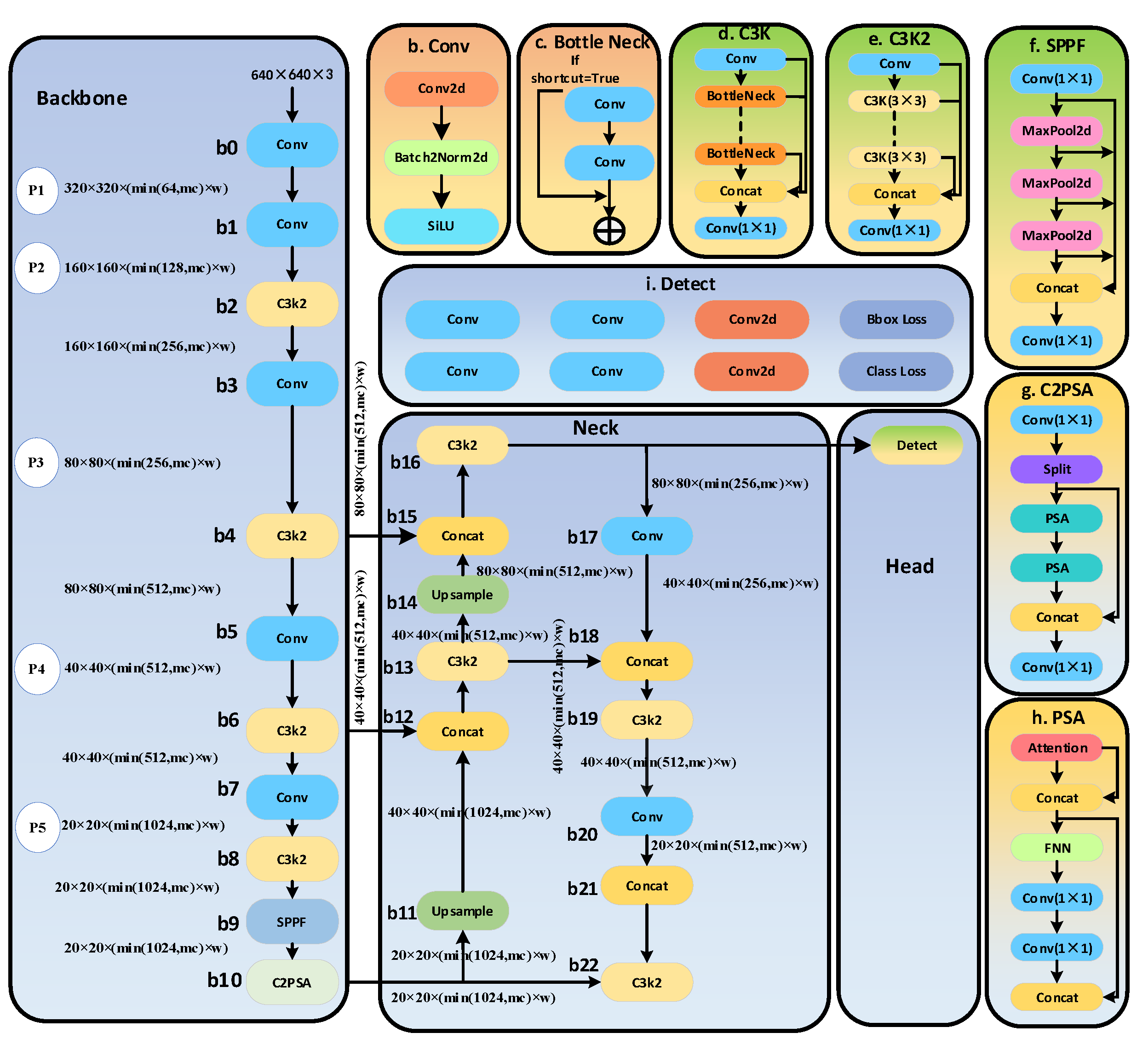
Figure 2.
CNN and Ghost Module,(a)operation of CNN,(b)operation of GhostModule.
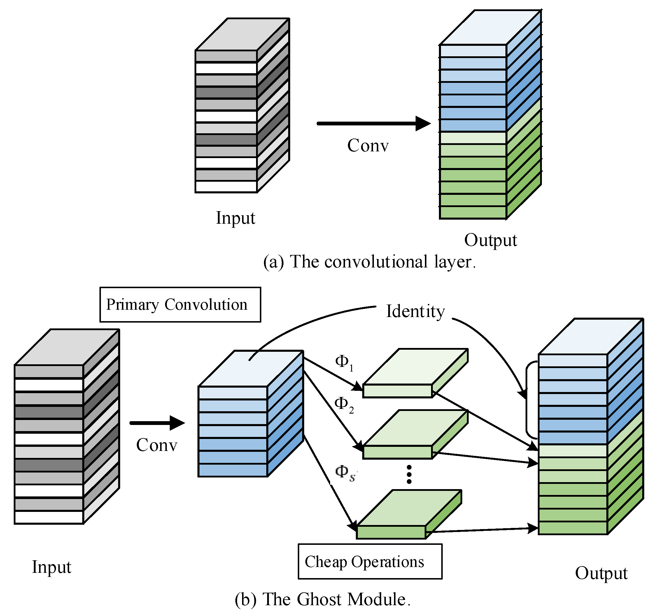
Figure 3.
Structure of GM-YOLOv11-backbone.
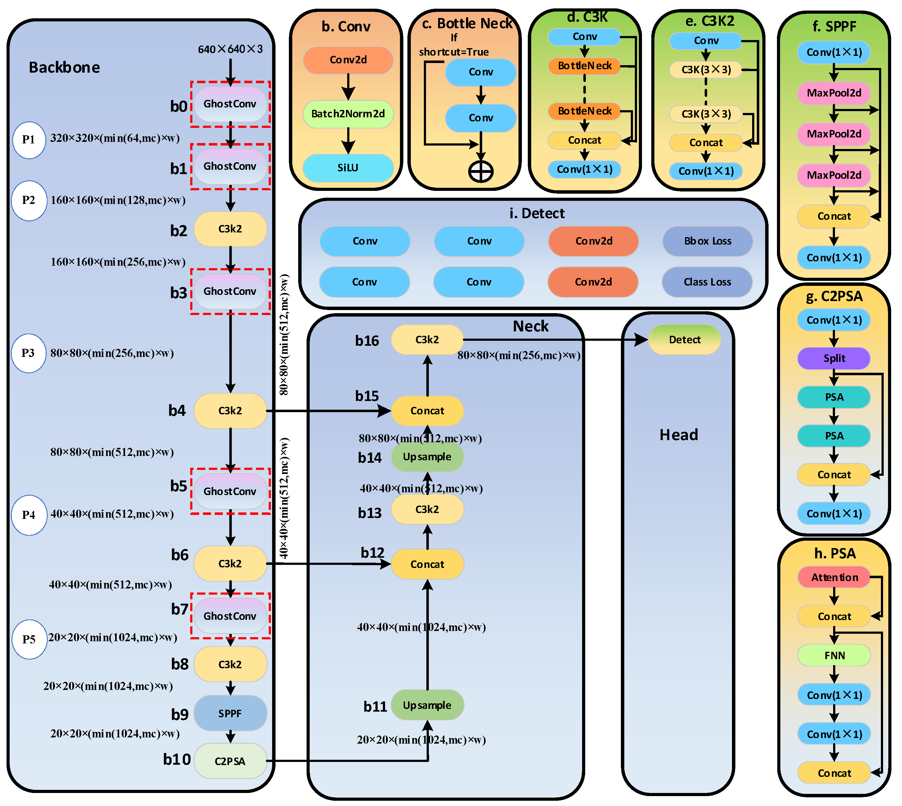
Figure 4.
Structure of GM-YOLOv11-head.
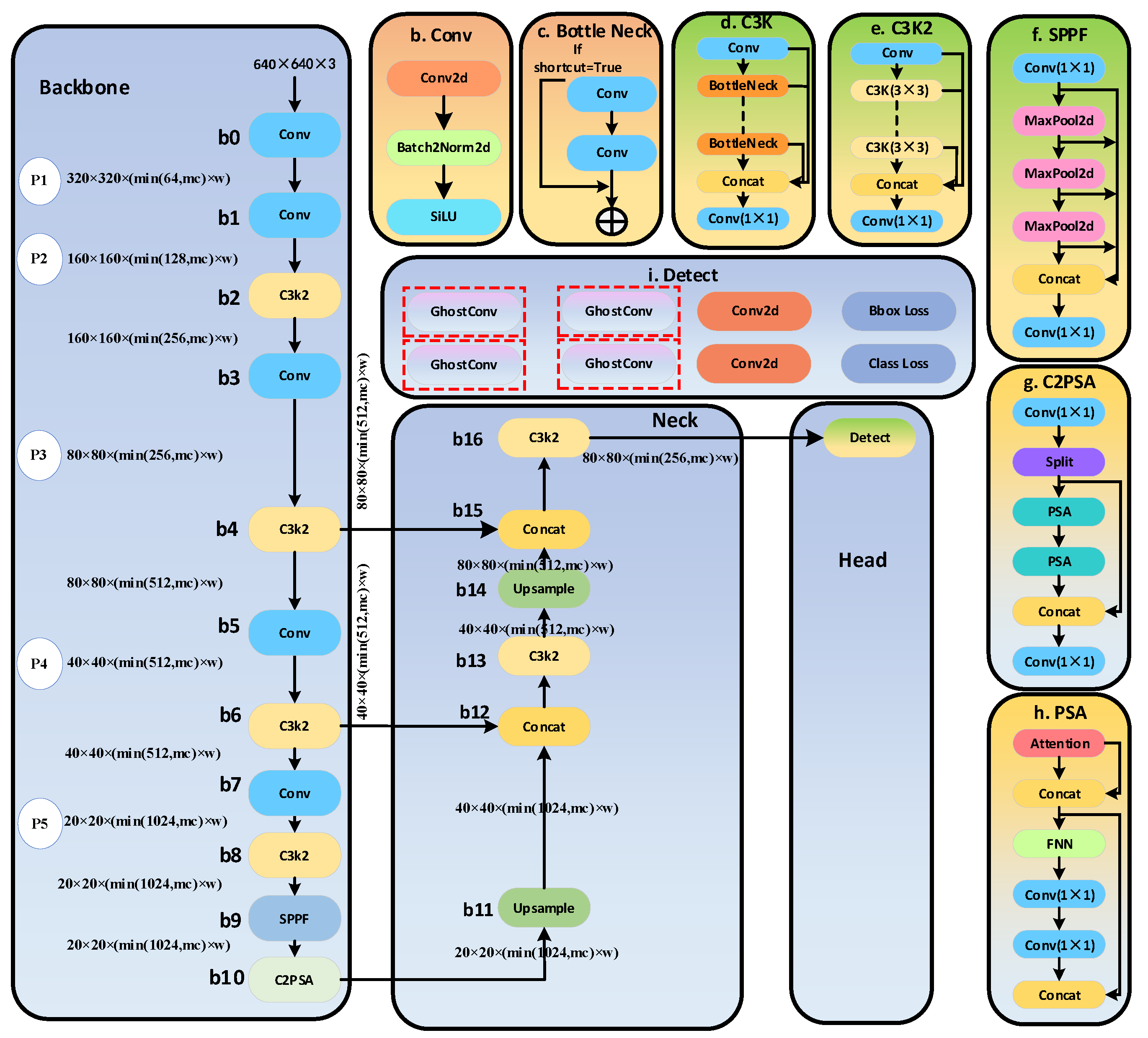
Figure 5.
Structure of GM-YOLOv11.
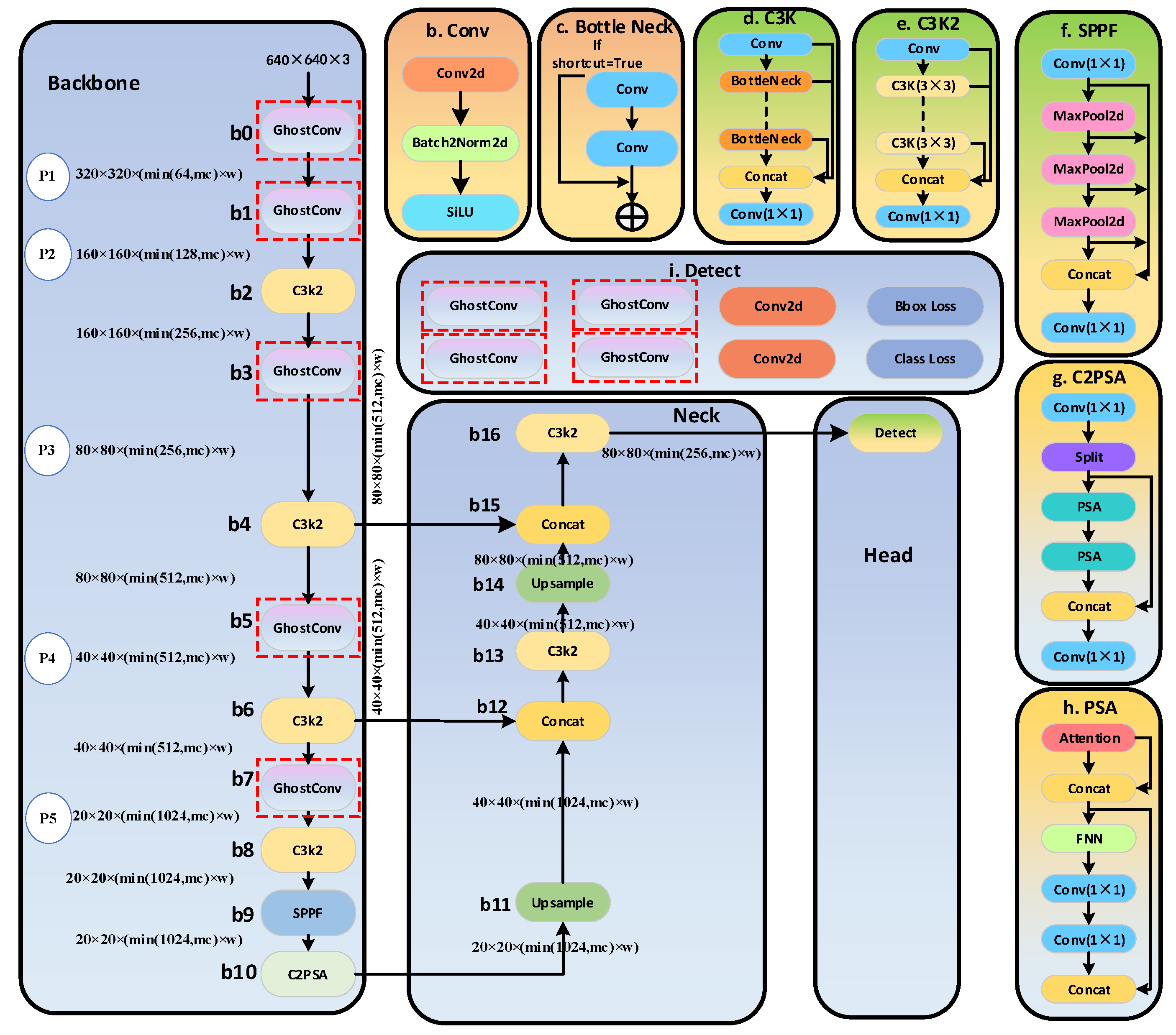
Figure 7.
Video-level Post-Processing Algorithm.
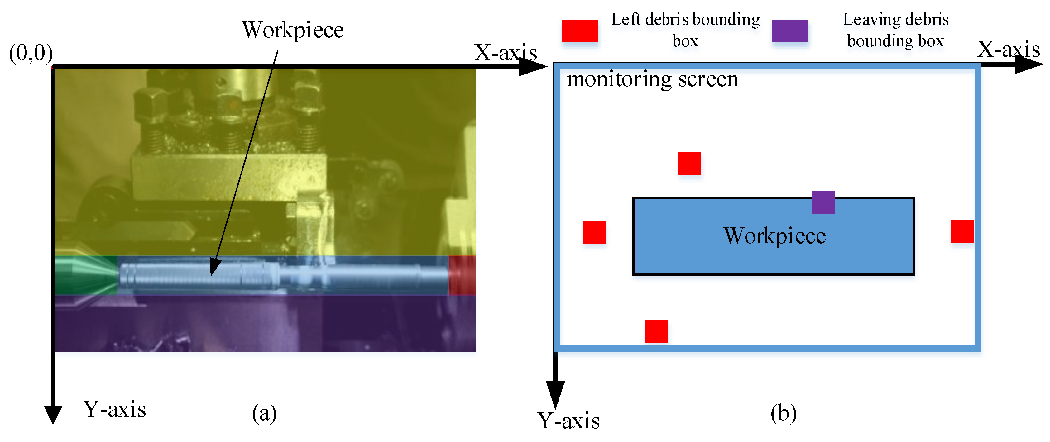
Figure 6.
Leaving debris and left debris (a)the workpiece processing site.(b)pixel size information.
Figure 6.
Leaving debris and left debris (a)the workpiece processing site.(b)pixel size information.
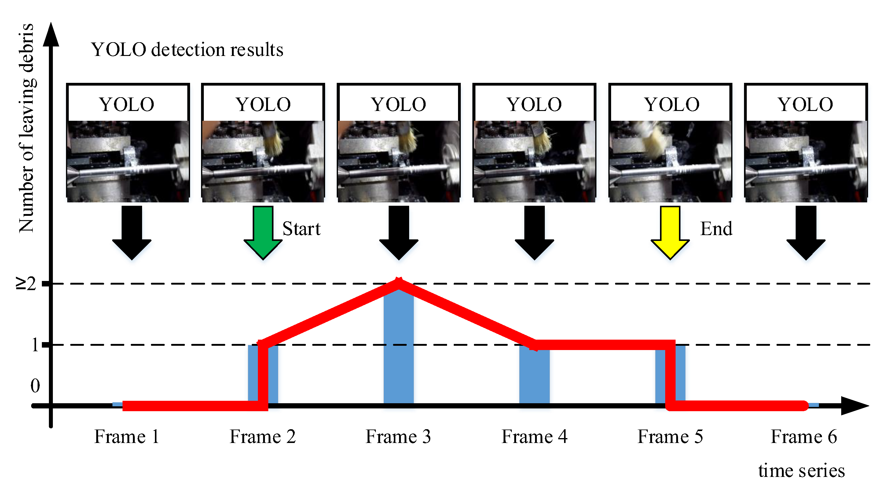
Figure 8.
Hip video data.
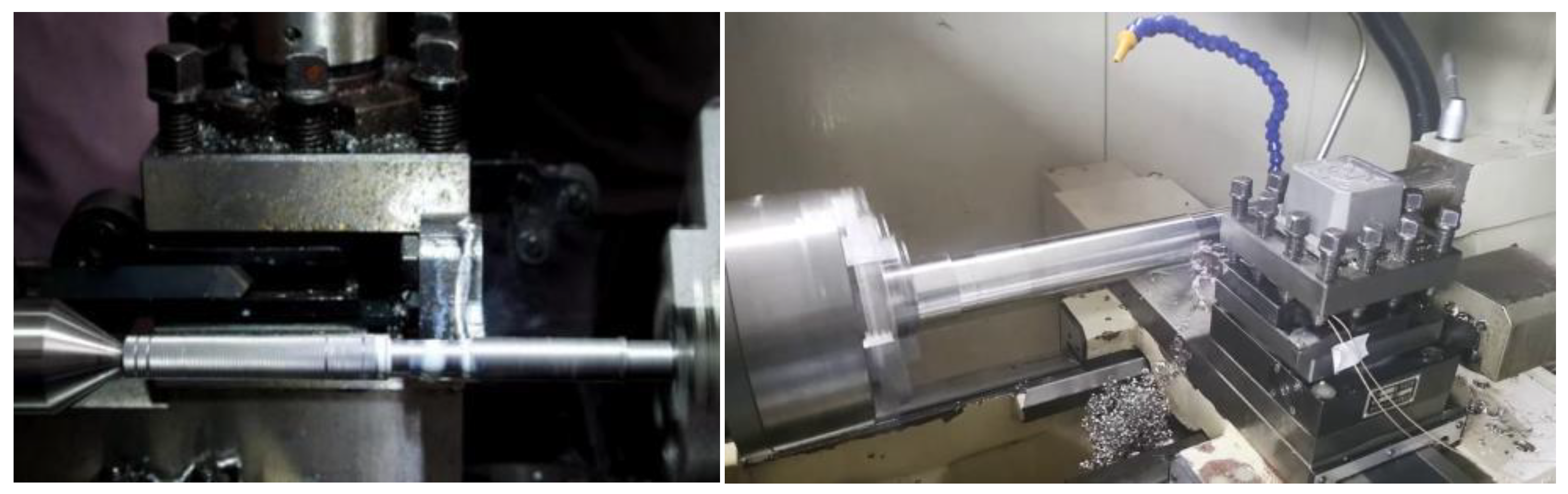
Figure 9.
Training loss and mAP@0.5 for YOLOv11n, GM-YOLOv11-backbone, GM-YOLOv11-head, and GM-YOLOv11,(a)training loss,(b)mAP@0.5.
Figure 9.
Training loss and mAP@0.5 for YOLOv11n, GM-YOLOv11-backbone, GM-YOLOv11-head, and GM-YOLOv11,(a)training loss,(b)mAP@0.5.
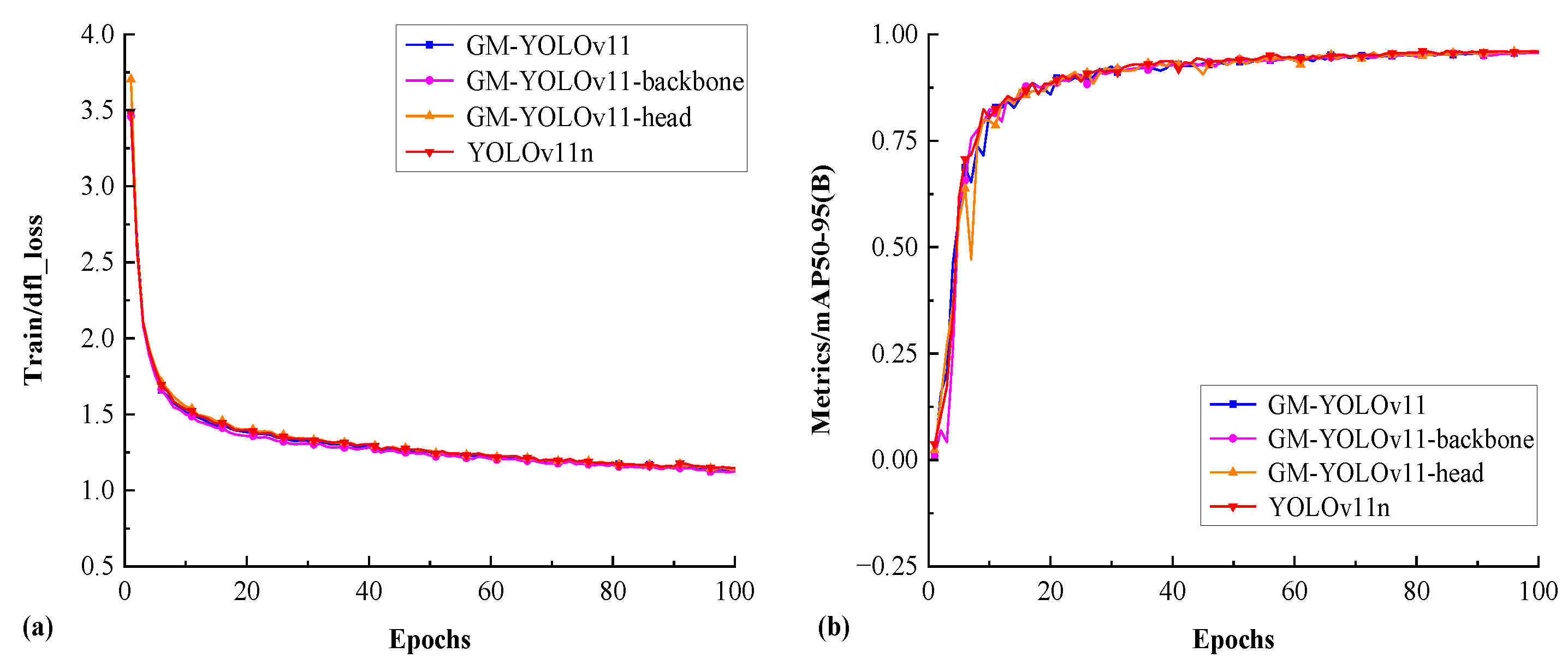
Figure 9.
Training loss and mAP@0.5 for YOLOv11n, GM-YOLOv11-backbone, GM-YOLOv11-head, and GM-YOLOv11,(a)training loss,(b)mAP@0.5.
Figure 9.
Training loss and mAP@0.5 for YOLOv11n, GM-YOLOv11-backbone, GM-YOLOv11-head, and GM-YOLOv11,(a)training loss,(b)mAP@0.5.
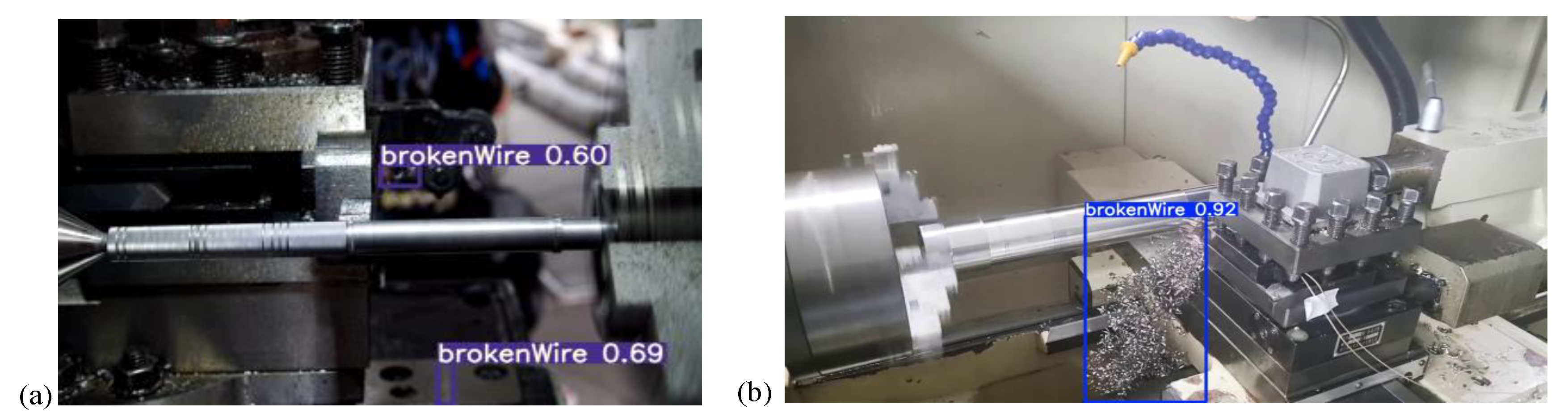

Table 1.
Algorithm of Dynamic Non-Maximum Suppression.
| Input: output of YOLO net#break#Output: all the debris and their location |
| (1)Findusing the standard Non-Maximum Suppression algorithm#break#(2)Adjust size ofaccording to Equations (7) (8) (9)#break#(3)find the bounding boxwith highest score ofaccording to Equation (10)#break#(4) calculate the IoU(,), as well as, if IoU(,)>delete bounding box#break#(5)Repeat sorting and soft threshold operation for the remaining predicted boundingbox and perform step(3) and(4) until no more boxes can be deleted. |
Table 2.
debris detection performance test results.
| Model | Precision#break#(%) | Recall#break#(%) | mAP@0.5#break#(%) | FLOPs#break#(G) | MS#break#(MB) | FPS |
| YOLOv5n | 92.66 | 92.44 | 91.10 | 7.73 | 1.9 | 116.68 |
| YOLOv8n | 90.22 | 88.72 | 89.53 | 8.75 | 3.2 | 149.02 |
| YOLOv9t | 89.67 | 90.12 | 92.24 | 8.23 | 2 | 73.78 |
| YOLOv10n | 91.14 | 86.66 | 87.05 | 8.57 | 2.3 | 100.2 |
| YOLOv11n | 94.11 | 95.42 | 94.68 | 6.48 | 2.6 | 154.34 |
| GM-YOLOv11-backbone | 93.60 | 94.08 | 93.63 | 5.81 | 2.2 | 167.34 |
| GM-YOLOv11-head | 93.36 | 93.67 | 93.66 | 6.33 | 2.5 | 156.23 |
| GM-YOLOv11 | 93.80 | 93.96 | 93.81 | 5.72 | 2 | 173.41 |
| Literature [25] | 92.27 | 91.69 | 90.12 | 6.44 | 1.7 | 146.34 |
| Literature [24] | 91.22 | 90.63 | 90.29 | 7.84 | 2.8 | 135.26 |
Table 3.
Partial Results from the Orthogonal Experiment on Hyperparameters in the DNMS Algorithm.
| regular parameters in Equation (10) | regular parameters in Equation (10) | left debris threshold | leaving debris threshold | Recall#break#(%) |
| 0.3 | 0.6 | 0.4 | 0.3 | 96.27 |
| 0.3 | 0.7 | 0.5 | 0.3 | 95.89 |
| 0.4 | 0.7 | 0.5 | 0.4 | 96.38 |
| 0.5 | 0.4 | 0.6 | 0.5 | 95.75 |
| 0.8 | 0.7 | 0.7 | 0.5 | 95.75 |
| 0.9 | 0.6 | 0.7 | 0.6 | 95.86 |
Table 4.
debris detection performance test results.
| Model | Precision#break#(%) | Recall#break#(%) | mAP@0.5#break#(%) |
| YOLOv5n+DNMS | 93.85 | 94.11 | 92.99 |
| YOLOv8n+DNMS | 93.30 | 90.78 | 90.85 |
| YOLOv9t+DNMS | 90.83 | 91.80 | 93.34 |
| YOLOv10n+DNMS | 92.46 | 88.33 | 88.89 |
| YOLOv11n+DNMS | 97.05 | 96.81 | 96.48 |
| GM-YOLOv11-backbone+DNMS | 95.13 | 96.18 | 95.08 |
| GM-YOLOv11-neck+DNMS | 94.81 | 94.37 | 95.01 |
| GM-YOLOv11+DNMS | 97.04 | 96.38 | 95.56 |
| Literature [25] | 92.27 | 91.69 | 90.12 |
| Literature [24] | 91.22 | 90.63 | 90.29 |
Table 5.
Details of the ten videos.
| Serial number | Duration (s) | Actual number of crack-debris |
| 1 | 36 | 13 |
| 2 | 103 | 47 |
| 3 | 158 | 61 |
| 4 | 210 | 82 |
| 5 | 213 | 79 |
| 6 | 213 | 80 |
| 7 | 51 | 25 |
| 8 | 49 | 18 |
| 9 | 35 | 24 |
| 10 | 28 | 7 |
| Total | 1096 | 436 |
Table 6.
Debris Quantity Counting Experiment.
| Model | Error proportion (%) |
| YOLOv5n+DNMS+VPPA | 11.93 |
| YOLOv8n+DNMS+VPPA | 15.37 |
| YOLOv9t+DNMS+VPPA | 13.07 |
| YOLOv10n+DNMS+VPPA | 13.30 |
| YOLOv11n+DNMS+VPPA | 9.63 |
| GM-YOLOv11-backbone+DNMS+VPPA | 10.55 |
| GM-YOLOv11-neck+DNMS+VPPA | 11.47 |
| GM-YOLOv11+DNMS+VPPA | 9.86 |
| Literature [25] + VPPA | 15.14 |
| Literature [24] + VPPA | 15.60 |
Disclaimer/Publisher’s Note: The statements, opinions and data contained in all publications are solely those of the individual author(s) and contributor(s) and not of MDPI and/or the editor(s). MDPI and/or the editor(s) disclaim responsibility for any injury to people or property resulting from any ideas, methods, instructions or products referred to in the content. |
© 2025 by the authors. Licensee MDPI, Basel, Switzerland. This article is an open access article distributed under the terms and conditions of the Creative Commons Attribution (CC BY) license (http://creativecommons.org/licenses/by/4.0/).
Copyright: This open access article is published under a Creative Commons CC BY 4.0 license, which permit the free download, distribution, and reuse, provided that the author and preprint are cited in any reuse.


