Submitted:
30 May 2025
Posted:
30 May 2025
You are already at the latest version
Abstract
In the obstacle grid map, due to the limited search directions of classical path algorithms and meta-heuristic algorithms, the shortest paths they solve are not true shortest paths (TSP), but rather shortest grid paths (SGP). In this paper, a SGP vertex extraction and filtering algorithm is proposed to extract and filter the key nodes in the SGP path, so as to obtain the TSP path under the same conditions. Experimental validation shows that the shortest path lengths found by the proposed SGP vertex extraction and filtering algorithm are shorter than those obtained by heuristic path algorithms, and it also outperforms recent new algorithms in comparative experiments. As the map scale increases and the obstacle rate rises, the advantages of this path algorithm become more pronounced.
Keywords:
the shortest grid path
; the true shortest path
; the obstacle grid map
1. Introduction
The shortest path problem is a fundamental issue in graph theory, and it has many different types. Depending on whether there are constraints, it can be divided into unconstrained shortest path problems and constrained shortest path problems. For example, the VPR (vehicle routing problem) is a typical constrained shortest path problem [1]. Based on the number of objectives, it can be categorized into single-objective shortest path problems and multi-objective shortest path problems. The TSP (Traveling Salesman Problem) problem is a classic example of a multi-objective shortest path problem [2]. Additionally, based on whether the constraints change, it can be classified as static or dynamic shortest path problem, among others. The concept of the shortest path is not limited to physical distance; it can also represent any quantifiable weight, such as time or cost. In practical applications, many problems can be transformed into shortest path problems for a solution.
Currently, algorithms for solving the shortest path problem can be roughly divided into classical path algorithms and heuristic path algorithms. Classical path algorithms are mainly used to solve small-scale deterministic problems, such as BFS, Dijkstra [3], DFS, etc., which have advantages when dealing with problems that have a unique optimal solution. Heuristic path algorithms are often used to solve large-scale complex problems, such as genetic algorithms (GA) [4], ant colony algorithms (ACO) [5], particle swarm optimization (PSO) [6], etc. These algorithms can effectively solve problems under multiple constraints and multi-objective problems [7]. Heuristic algorithms can also be categorized into several different types based on their principles, namely population-based algorithms, physics-based algorithms, and evolutionary algorithms [8,9,10].
In recent years, research on the shortest path has been abundant. For example, [11] models practical problems as weighted time path graphs and proposes a graph transformation technique based on BFS and Dijkstra algorithms to study the shortest time paths in these graphs. In [12], a greedy strategy from the Dijkstra algorithm is used to propose a baseline algorithm, which combines the lower bound of the shortest path and the lower bound of the multi-path to form a framework for solving the K shortest path problem, capable of finding the first k distinct shortest paths in a directed weighted graph. [13] introduces an innovative genetic algorithm to solve the clustering shortest path tree (CluSPTP) problem and tests it on both Euclidean and non-Euclidean instance sets. [14] proposes an improved distance-based ant colony optimization path (IDBACOR), incorporating direction information during pheromone updates and adding a speed factor in probability calculations, guiding ants to move as close as possible toward the target point, thus addressing the shortest path problem in transportation networks. However, in reality, the shortest paths found by these algorithms still have space for optimization.
In path planning, the length of the route is typically the most critical metric, as its size directly impacts the cost incurred. For instance, in constructing roads or bridges, every additional meter can significantly increase costs. In autonomous vehicle navigation, the length of the chosen route directly affects the vehicle's energy consumption. Therefore, effectively reducing the path length is a very important issue.
However, in two-dimensional obstacle grid maps, some existing algorithms fail to find the optimal solution effectively. Classic pathfinding algorithms such as BFS and Dijkstra do not solve the shortest path but rather the shortest grid path (SGP). There is room for optimization in this path, which increases with the distance between the start and end points. Heuristic pathfinding algorithms like GA, ACO, and PSO can find shorter paths than classic pathfinding algorithms in close proximity, but once the distance between the start and end points increases, the efficiency of these heuristic algorithms significantly decreases, and their solution quality may even be inferior to that of classic pathfinding algorithms.
In view of the above situation, this paper proposes a SGP vertex extraction and filtering algorithm (SGP vertexs extraction filtering algorithm, SGPVEFA) to solve the real shortest path in the two-dimensional obstacle grid graph. The innovation points of this paper are as follows.
A method to optimize SGP into TSP is proposed.
An obstacle grid vertex extraction algorithm based on the equivalent path is proposed.
A path optimization method based on an improved dynamic optimization algorithm is proposed.
Subsequent experiments have shown that SGPVEFA can efficiently optimize the SGP path into a true shortest path, regardless of map size and distance between starting and ending points. In long-distance situations, the advantages of SGPVEFA are even more significant.
2. The True Shortest Path in the Obstacle Grid Map
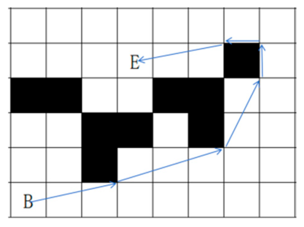
The shortest path problem in a grid map can typically be solved using various algorithms, including but not limited to backtracking, Dijkstra algorithm, and dynamic programming. However, these algorithms usually explore only 4 or 8 directions, which results in the shortest path not being the true shortest path (TSP), but rather the shortest grid path (SGP) [15]. As shown in Figure 1, path a represents SGP, while path b represents TSP. In this paper, SGP refers to the shortest path from the starting point to the endpoint through continuous movement in 8 directions.
In the obstacle grid map, due to the limitations of obstacles, one must take a longer route to reach the destination. Most path search algorithms can only move in 8 directions, with each step landing at the center point of the grid. However, TSP requires movement along the boundaries or vertices of obstacles, allowing for movement in any direction. The limitation on search directions creates the difference between SGP and TSP. However, searching at each vertex of an obstacle would require a significant amount of time.
In the unobstacle map, when the starting point and the endpoint are on the same row or column, SGP and TSP are exactly the same. However, when the destination is offset, there will be a difference between SGP and TSP. The reason is that SGP can only turn at 45-degree angles, while TSP can turn at any angle. For the obstacle grid map, the movement Angle of TSP will also be limited. It can no longer go directly from the starting point to the end point, but instead moves around the obstacles by sticking to the obstacles. Therefore, the process of optimizing SGP into TSP is the process of sticking to the boundary of obstacles in SGP.
Since SGP is the shortest path limited to 8 directions and TSP is the shortest path allowed to move in any direction, the routes and grids selected by SGP and TSP are roughly the same when bypassing obstacles. We also notice that SGP avoids obstacles through multiple diagonal movements, which intersect with obstacle vertices in a series of obstacle vertices. The lines connecting these obstacle vertices precisely form the TSP. Therefore, optimizing SGP to TSP only requires focusing on the obstacle vertices passed during each turn. However, in complex obstacle grid maps, not all obstacle vertices passed during turns are included in the TSP. The set of path points in the TSP is a subset of the set of obstacle vertices, so it is necessary to filter out the valid path points that constitute the TSP.
Figure 2.
The TSP consists of the line connecting the obstacle vertices.
Therefore, this paper designs an SGP vertex extraction and filtering algorithm. By constructing equivalent paths, the obstacles passed by SGP are extracted and modeled as a chain structure. Then, the improved dynamic programming algorithm is used to filter and optimize it into TSP. The overall flow chart of SGPVEFA is shown in Figure 3.
3. Obstacle Vertex Extraction Algorithm Based on Equivalent Path
3.1. Problem Modeling
Let G be an grid graph containing a set of obstacles O and a set of passable grids A, where x is any grid in it, that is, , and . There is an SGP in A and it’s from the starting point B to the endpoint E passing through n nodes. Here, represents that is the grid center of the row and the column in G, and can be obtained by moving one step in eight directions. The objective function is the total path length of S, which can be calculated by Formula (1).
The following constraints must be satisfied for formula (1):
That is, all nodes must not cross the boundary.
That is, every move is an 8-direction move.
That is, can't stagnate at a certain point.
That is, there can be no loops in the path.
The requirement is to optimize S into the TSP path from B to E , so that is minimized.
3.2. Equivalent Path
Assuming that in the grid graph G, under the premise of only allowing 8 directions to move, the shortest path from the starting point B to the end point E requires m horizontal movements and n diagonal movements, then the relative order of these movements can be adjusted arbitrarily without affecting the arrival at the destination, which is called these paths are equivalent paths in this paper.
Figure 4.
Equivalent path.
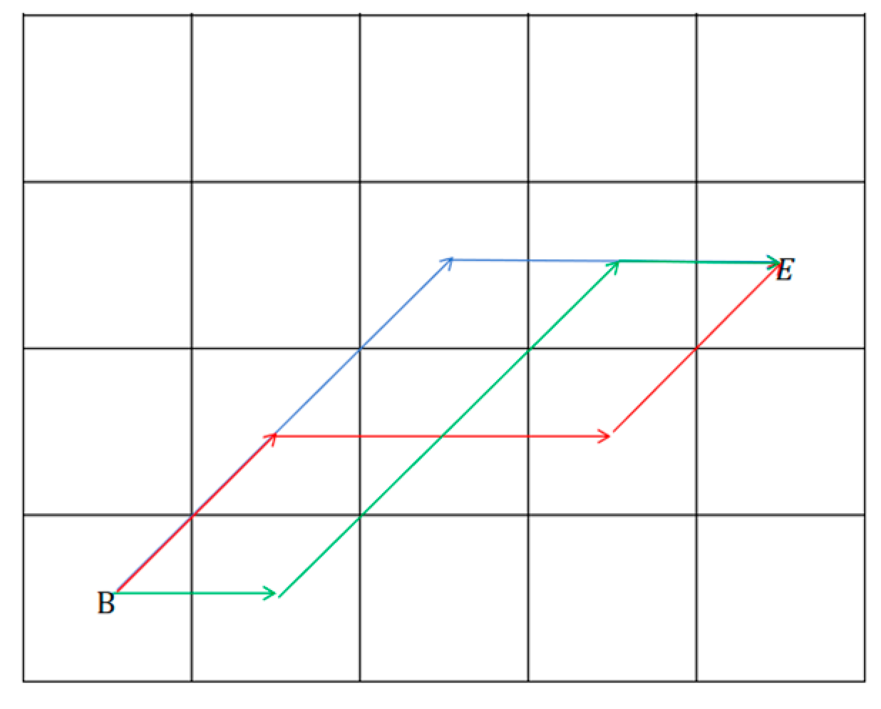
A continuous 8-directional movement path in a barrier grid can be decomposed into several combinations of equivalent paths. As shown in Figure 5, the continuous 8-directional movement path from grid B to grid E can be divided into 3 segments. Among them, a and c have two path combinations respectively, which are equivalent paths to each other, while b can be regarded as a special equivalent path with a path combination number of 1.
3.3. Obstacle Vertexs Extraction Algorithm (OVEA)
The trajectory of an SGP varies depending on the distribution of obstacles. Directly searching for all obstacle vertices traversed by the entire SGP is extremely difficult, so it is necessary to break down the SGP. An SGP consists of several 8-directional movements, which can be divided into two types: movement along the coordinate axes (referred to as axial movement in this paper) and movement along the diagonals (referred to as diagonal movement in this paper). Axial movements do not pass through obstacle vertices; only diagonal movements may encounter them. Therefore, extracting obstacle vertices requires focusing on the diagonal movements within the SGP.
We also noticed that there are three possible continuous movements in the SGP path: Axial-oblique movement, Oblique-axial movement, and Oblique-oblique movement (Axial-Axial movement can be optimized at turns, which contradicts the definition of SGP). This means that in SGP, at least one of any two consecutive movements is an oblique movement. Based on this finding, we sequentially decompose a complete SGP into these three types of movement combinations and perform obstacle vertex extraction for each pair of consecutive movements.
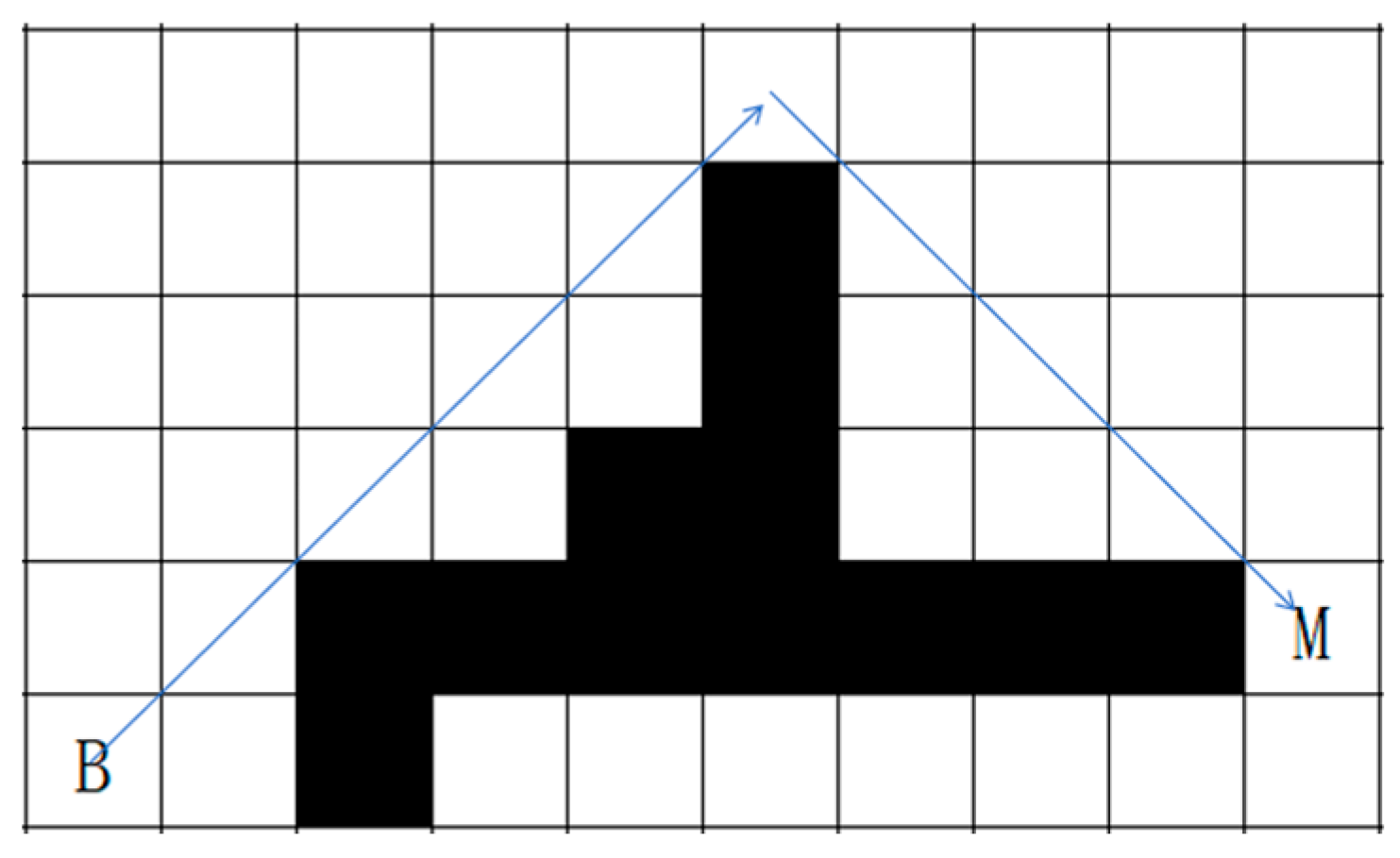
3.3.1. Axial-Oblique Movement
Assuming in a SGP, from grid B to grid M, there are m consecutive axial moves and n consecutive diagonal moves in the same direction. The starting point of each is (), and the endpoint is (). We try to move in the reverse direction of the axial movement with each diagonal movement to construct an equivalent path until we hit the obstacle vertex or move to the extension of the previous equivalent path, as shown in Figure 6.
Assuming the starting point of n i after translation is grid (), and the endpoint is grid (), we will sequentially check the four grids: (),(),(), and (). If only one of these four grids is an obstacle grid, we consider to have stopped due to touching an obstacle vertex. When , we consider to have stopped because it has moved onto the extension of the previous equivalent path.
After the equivalent path is constructed, for the equivalent path that stops due to touching the obstacle vertex, we add the obstacle vertices it passes in the order of sequence into the TSP candidate point set.
3.3.2. Oblique-Axial Movement
For oblique-axial movement, we can consider it as the reverse operation of axial-oblique movement. Due to the reversibility of the path, the obstacle vertices traversed by a forward and backward movement along an SGP are the same. Assuming in an SGP, from grid B to grid M, there are m consecutive oblique movements and n consecutive axis movements . If we flip this segment, the path transforms into one from grid M to grid B {,,,}, and then we can apply the method for axial-oblique movement described in Section 3.3.1 to extract the obstacle vertices encountered and add them to the candidate point set in reverse order.
Figure 7.
The Oblique-axial movement is reversed to the axial-oblique movement.

3.3.3. Oblique-Oblique Movement
For oblique-oblique movement, we can consider it as oblique-axial(number of moves is 0)-oblique movement. The first half of the oblique-axial movement should be reversed according to the strategy in 3.3.2 to construct an equivalent path. Since the number of axial movements is 0, the whole path itself is an equivalent path. Similarly, the equivalent path constructed by the axial-oblique movement in the second half is itself.
Therefore, for oblique-oblique movement, we only need to record the obstacle vertices that pass through it and add them to the candidate point set.
Figure 8.
Oblique-oblique movement.
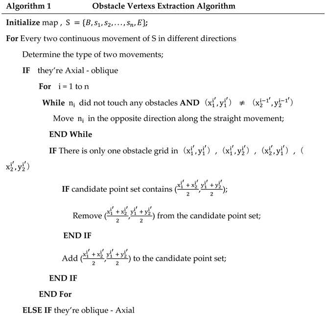
The pseudocode of the obstacle vertex extraction algorithm is shown in Algorithm 1.
 |
4. Path Smoothing Method Based on Improved Dynamic Programming Algorithm
After extracting all the obstacle vertices that SGP has passed through, we found that not all of these points are included in the TSP path. There may be some non-adjacent but directly connectable points, as shown in Figure 9(c). Therefore, the original problem is transformed into screening points from the candidate set, removing path points outside the TSP path to achieve a smoother path.
Due to the obstacle vertices being added to the candidate point set through translational contact with obstacles and added in the order of SGP paths, adjacent candidate points can be directly connected. Therefore, the points in the candidate point set satisfy the data structure shown in Figure 10, where all points form a one-way linked list according to their order of addition to the candidate point set. Since there are some path points that can be directly connected, some path points have one or more branches, and the length of these branches does not exceed the length of the main chain.
4.1. Problem Transformation Modeling
It is known that the set of candidate points with length is . Find a subsequence in with length such that (6) formula holds.
P and Q should satisfy the following constraints:
That is, Q is a subset of P.
That is, the path length of the branch is not greater than that of the main chain.
4.2. Improve the Dynamic Programming Algorithm
The following proves the feasibility of using dynamic programming algorithm for this problem.
Lemma 1
. If is the shortest path from v 1 to v k, then for any two nodes and in the path, the path is also the shortest path from to .
Proof of Lemma 1
: Since Q is the TSP path from B to E, Lemma 1 indicates that Q possesses the property of optimal substructure. Suppose there is a common point in P and Q, and . Then, the subsequence of Q forms the TSP path from B to , and the subsequence of Q forms the TSP path from to E. According to the definitions of P and Q, is a subsequence of , and is a subsequence of . This means that the optimal solution to this problem can be broken down into the optimal solutions of its subproblems. In summary, this problem also possesses the property of optimal substructure, so it can be solved using dynamic programming algorithms.□
Due to the fact that this problem not only requires obtaining the path length but also storing the shortest path, an additional array is needed during the dynamic programming process to record the historical optimal paths. However, as the algorithm runs, the number of nodes in the historical optimal path continues to increase, meaning the array length is constantly changing, which is not conducive to pre-allocating space. Moreover, when the problem scale is large, it requires more space for storage. To address this issue, we leverage the characteristic of optimal substructures in candidate point sets and set up an auxiliary array to store predecessor node indices instead of storing paths. As shown in Figure 11.
It is also noted that the candidate point set has the following properties:
Property 1
: The subsequent adjacent points of a point in the candidate set extracted by the SGP path are continuous in the candidate set.
Proof of Property 1 (reductio ad absurdum)
: Suppose that the subsequent adjacent points of a candidate point in the candidate set of a SGP path are discontinuous in the set, that is, there exists a continuous subsequence , where are adjacent points, A and C are not adjacent points, D is a subsequent candidate point of C, and A and D are adjacent points.
Because A and C are not adjacent points, the line connecting A and C must pass through some obstacle. The boundary points between A and this obstacle form two straight lines, a and b, as shown in Figure 12. Since A and D are adjacent points, D should be located outside of a and b. If D is on the outside of a, due to the adjacency between A and D, the line AD does not pass through the obstacle or the wall gap, so there exists a shorter SGP between AD that does not need to bypass the obstacle between AC, which contradicts the definition that the SGP is the shortest path in 8 directions. Similarly, if D is on the outside of b, there also exists a shorter SGP, leading to another contradiction. In conclusion, A and D are not adjacent points, thus, Property 1 holds.□
Inference 1
: For any two nodes and () in the candidate point set , where the set of pre-adjacent points of is and the set of pre-adjacent points of is , if , then .
Proof of Inference 1 (Proof by Contradiction)
: Assume and . According to Property 1, the set of adjacent points after is , and the set of adjacent points after is . Since and , it follows that , so and are adjacent points. Furthermore, since , , which contradicts . Therefore, Inference 1 holds.□
Inference 1 indicates that the boundary of the set of previous adjacent points for a path point will shift backward as the point moves further in the candidate point set. Therefore, a sliding window can be used to optimize dynamic programming algorithms, thereby improving algorithm efficiency. The sliding window is used to define the range of the set of previous adjacent points, and it gradually advances toward the endpoint with each iteration.
The pseudocode of the optimized dynamic programming algorithm is shown in Figure 13.
5. Experiment
5.1. Experimental Environment
All experiments in this paper were conducted using MATLAB R2023a software on a computer with 16GB of RAM and a 2.20 GHz processor. The maps used for all experiments were randomly generated by the system based on the input map side length N, forming an N×N grid matrix. Obstacle grids were randomly selected according to the input obstacle rate ρ. Both the x and y coordinates of the starting point and endpoint were generated by taking random positive integers within the range of 0 to N.
5.2. Ablation Experiment
To test the effectiveness and importance of each part of SGPVEFA, this paper sets up ablation experiments. The test subjects include the basic algorithm (Basic), the obstacle vertex extraction algorithm (OVEA), and the path smoothing method (PSM). The comparison algorithm is the SGP vertex extraction filtering algorithm (SGPVEFA). Here, the basic algorithm refers to performing only SGP path search without path optimization.
The experiment randomly generates 100 maps, with the map side length N increasing from 100 to 1000, with each increment being 100. For each N, 10 maps are randomly generated, and for each map, obstacle grids and start/finish points are randomly generated, with an obstacle rate set at 0.3. The changes in path length of sub-algorithm ablation experiments as the map side length N increases are shown in Figure 14, and the changes in search time as the map side length N increases are shown in Figure 15. Since the search time approaches 0 when the map side length is too small, only the search times for are provided in Figure 15.
From Figure 14, it can be seen that if obstacle vertices are not extracted and path smoothing is performed directly, the total path length can be reduced to a certain extent, but it cannot be optimized. If only obstacle vertices are extracted without performing path smoothing, it may even lead to an increase in the total path length. Only when both parts operate simultaneously can the path length be optimized. According to Figure 15, the time consumed by SGPVEFA is very limited, almost negligible compared to the search time of SGP paths.
The ablation experiments show that SGPVEFA is very efficient and can find the optimal path.
5.3. Comparison Experiment of Intelligent Path Planning Algorithms
In order to test the performance of SGPVEFA compared with other path planning algorithms, we set up a comparative experiment, and the comparison object is the intelligent path planning algorithm (GA, GWO [16], DE [17], PSO, SSA [18], etc.). We will conduct a comparative experiment from two aspects: map size and obstacle rate.
5.3.1. Map Size
In the experiment, 7 sets of grid maps were randomly generated, and the length of the map N increased from 100 to 700, with an increment of 100 each time. The obstacle grid and starting point (ensuring a feasible solution) were randomly generated on each map, and the obstacle rate ρ was set to 0.1.
The algorithm parameters are set as follows: the maximum number of iterations is set to 100, and the population size is set to 50. The crossover probability pc for GA is 0.8, and the mutation probability . For GWO, the initial value of a is 2, decreasing to 0 with each iteration. The DE mutation probability f is a random number between [0.2, 0.8], and the crossover probability . For PSO, the inertia weight , the individual learning factor , and the group learning factor . The SSA explorer ratio .
The path length of each algorithm changes with the map edge length N as shown in Figure 16, and the search time changes with the map edge length N as shown in Figure 17. Since the search time approaches 0 when the map edge length is too small, only the search time when is given in Figure 17.
Experiments show that SGPVEFA has obvious advantages in terms of path length, and the advantage is more significant with the increase of N. In terms of search time, SGPVEFA's search time is slightly shorter than that of intelligent path planning algorithms when N is small, and with the increase of N, the search time of SGPVEFA is basically equal to that of intelligent path planning algorithms (except GA).
5.3.2. Obstacle Rate
Due to the presence of numerous obstacles, intelligent optimization algorithms may fail to find feasible solutions. Therefore, we conducted comparative experiments on the success rates and solution quality of various algorithms under three different obstacle densities. The success of an algorithm is marked by successful population initialization and finding a feasible solution within the specified number of iterations. The experiment randomly generated 3 sets of grid maps, with each set containing 50 maps. Each map has a side length of 500×500, and the obstacle density ρ was set at 0.1, 0.2, and 0.3, respectively. Obstacle grids and start/finish points were randomly generated on each map (ensuring there is a feasible solution). The parameter settings for each algorithm are the same as in Section 5.3.1. The success rate test results for each algorithm are shown in Table 1. In cases where the algorithms succeeded, the comparison of path lengths, search times, and SGPVEFA is presented in Table 2, Table 3, Table 4, Table 5 and Table 6.
As shown in Table 1, the algorithm proposed in this paper can still accurately find feasible solutions for complex maps. However, as the obstacle rate increases, the success rate of the intelligent optimization algorithm drops significantly. When the obstacle rate reaches 0.3, the success rate is below 10%, and for GA, it is only 2%, making it almost impossible to find a solution. This highlights the superiority of SGPVEFA in high-obstacle-rate environments. Tables 2 to 6 show that under three different obstacle rates, the search time and path length found by SGPVEFA are shorter than those achieved by the intelligent optimization algorithm.
5.4. Comparative Experiments with New Algorithms in Recent Years
We also conducted comparative experiments with some path planning algorithms proposed in recent years, such as the improved artificial bee swarm algorithm (IABC) proposed by [19] and the improved butterfly optimization algorithm (IBOA) proposed by [20].
5.4.1. Compared with IABC
We tested SGPVEFA using maps from the same environment as in [19], comparing the test results with those in [19]. The IABC parameters were set as follows: maximum number of iterations is 200, initial population size is 50, and maximum population size is 100. The four environmental map settings are: a simple environment with regular obstacles (Environment 1, obstacle rate 0.19), a complex environment with regular obstacles (Environment 2, obstacle rate 0.26), a simple environment with random obstacles (Environment 3, obstacle rate 0.17), and a complex environment with random obstacles (Environment 4, obstacle rate 0.22). The paths found by the two algorithms under different environments are shown in Figure 18, and Table 7 provides the mean path lengths and node counts, optimal values, and standard deviations for the two algorithms. SGPVEFA is an exact algorithm, yielding consistent results each time it runs.
Experimental results show that, whether in simple or complex obstacle environments, the path found by SGPVEFA is smoother compared to IABC, with fewer turns and nodes, and a shorter path length. Moreover, in complex obstacle environments, the path found by IABC may pass through wall gaps, whereas SGPVEFA avoids such situations, making it safer in real-life production and daily use.
5.4.2. Compared with IBOA
We tested SGPVEFA using the same environment map from [20], comparing the test results with those in [20]. The IBOA parameters were set as follows: maximum number of iterations is 50, population size is 4000, and two path simplification strategies proposed in [20] were adopted. On a complex obstacle map of 40x40 size, the paths found by the two algorithms are shown in Figure (19), and the path lengths and node counts are listed in Table 8.
Experiments show that SGPVEFA still has advantages over IBOA with the combined path simplification strategy in terms of path length and fewer path nodes, which makes the path searched by SGPVEFA smoother and with fewer turns.
6. Summary
This paper proposes a SGP vertex extraction and filtering algorithm for optimizing the shortest grid path in an obstacle grid map to the true shortest path. It can search for a shorter and smoother path than intelligent path planning algorithms in a short time. In large-scale maps and high obstacle rates, SGPVEFA performs particularly well.
But SGPVEFA can currently only solve problems with obstacle grid maps. In practical scenarios, the problem needs to be modeled in a similar manner, which is no easy task. Additionally, SGPVEFA is a static algorithm; in real life, obstacles and feasible paths may change over time, requiring some dynamic response mechanisms. Furthermore, the problems we encounter in real life are not limited to two-dimensional planes. For example, drone path planning, we can attempt to extend SGPVEFA to three-dimensional space in future research.
Funding
This study was funded by National Natural Science Foundation of China (Grant No: 62402200).
Institutional Review Board Statement
Not applicable.
Informed Consent Statement
Not applicable.
Data Availability Statement
The data used in this study are all randomly generated.
Conflicts of Interest
This study does not have any conflicts of interest with any organization or individual.
References
- Braekers, K., Ramaekers, K., & Van Nieuwenhuyse, I. (2016). The vehicle routing problem: State of the art classification and review. Computers & Industrial Engineering, 99(open in a new window), 300–313. [CrossRef]
- Pop, P. C., Cosma, O., Sabo, C., & Sitar, C. P. (2024). A comprehensive survey on the generalized traveling salesman problem. European Journal of Operational Research., 314(open in a new window)(3(open in a new window)), 819–835. [CrossRef]
- Dijkstra, E.W. A note on two problems in connexion with graphs. In Edsger Wybe Dijkstra: His Life, Work, and Legacy; Association for Computing Machinery: New York, NY, USA, 2022; pp. 287–290. [Google Scholar]
- Holland, J.H.: Genetic algorithms. Sci. Am. 267(1), 66–73 (1992).
- Colorni, Alberto, Marco Dorigo, and Vittorio Maniezzo. "An Investigation of some Properties of an" Ant Algorithm"." Ppsn. Vol. 92. No. 1992. 1992.
- J. Kennedy and R. Eberhart, "Particle swarm optimization," Proceedings of ICNN'95 - International Conference on Neural Networks, Perth, WA, Australia, 1995, pp. 1942-1948 vol. [CrossRef]
- Katona, K.; Neamah, H.A.; Korondi, P. Obstacle Avoidance and Path Planning Methods for Autonomous Navigation of Mobile Robot. Sensors 2024, 24, 3573. [Google Scholar] [CrossRef] [PubMed]
- Hussain, K. , Mohd Salleh, M.N., Cheng, S. et al. Metaheuristic research: a comprehensive survey. Artif Intell Rev 52, 2191–2233 (2019). [CrossRef]
- Reeves, C. Landscapes, operators and heuristic search. Annals of Operations Research 86, 473–490 (1999). [CrossRef]
- Yahia, H.S. , Mohammed, A.S. Path planning optimization in unmanned aerial vehicles using meta-heuristic algorithms: a systematic review. Environ Monit Assess 195, 30 (2023). [CrossRef]
- H. Wu, J. Cheng, Y. Ke, S. Huang, Y. Huang and H. Wu, "Efficient Algorithms for Temporal Path Computation," in IEEE Transactions on Knowledge and Data Engineering, vol. 28, no. 11, pp. 2927-2942, 1 Nov. 2016. [CrossRef]
- H. Liu, C. Jin, B. Yang and A. Zhou, "Finding Top-k Shortest Paths with Diversity," in IEEE Transactions on Knowledge and Data Engineering, vol. 30, no. 3, pp. 488-502, 1 March 2018. [CrossRef]
- Cosma, P. C. Pop and I. Zelina, "An Effective Genetic Algorithm for Solving the Clustered Shortest-Path Tree Problem," in IEEE Access, vol. 9, pp. 15570-15591, 2021. [CrossRef]
- Raghu Ramamoorthy (2020) An improved distance-based ant colony optimization routing for vehicular ad hoc networks, International Journal of Communication Systems, 33 (14). [CrossRef]
- Bailey JP, Nash A, Tovey CA et al (2021) Path-length analysis for grid-based path planning. Artif Intell 301:103560.
- Mirjalili, S., Mirjalili, S.M., Lewis, A.: Grey wolf optimizer. Adv. Eng. Softw. 69, 46–61 (2014).
- Storn, R., Price, K. Differential Evolution – A Simple and Efficient Heuristic for global Optimization over Continuous Spaces. Journal of Global Optimization 11, 341–359 (1997). [CrossRef]
- Xue, J., & Shen, B. (2020). A novel swarm intelligence optimization approach: sparrow search algorithm. Systems Science & Control Engineering, 8(1), 22–34. [CrossRef]
- Yildirim, Mustafa Yusuf, and Rustu Akay. "An efficient grid-based path planning approach using improved artificial bee colony algorithm." Knowledge-Based Systems (2025).
- Zhai, Rongjie, et al. "Application of improved butterfly optimization algorithm in mobile robot path planning." Electronics 12.16 (2023): 3424.
- Author 1, A.B. Title of Thesis. Level of Thesis, Degree-Granting University, Location of University, Date of Completion.
- Title of Site. Available online: URL (accessed on Day Month Year).
Figure 1.
SGP and TSP.

Figure 3.
Algorithm flow chart of SGPVEFA.
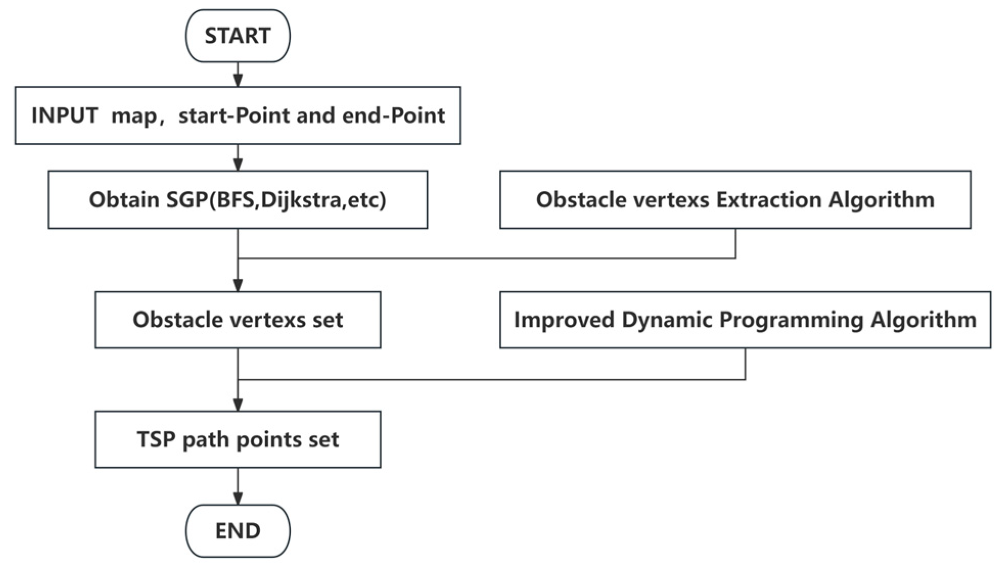
Figure 5.
The 8-direction path can be divided into several equivalent path combinations.
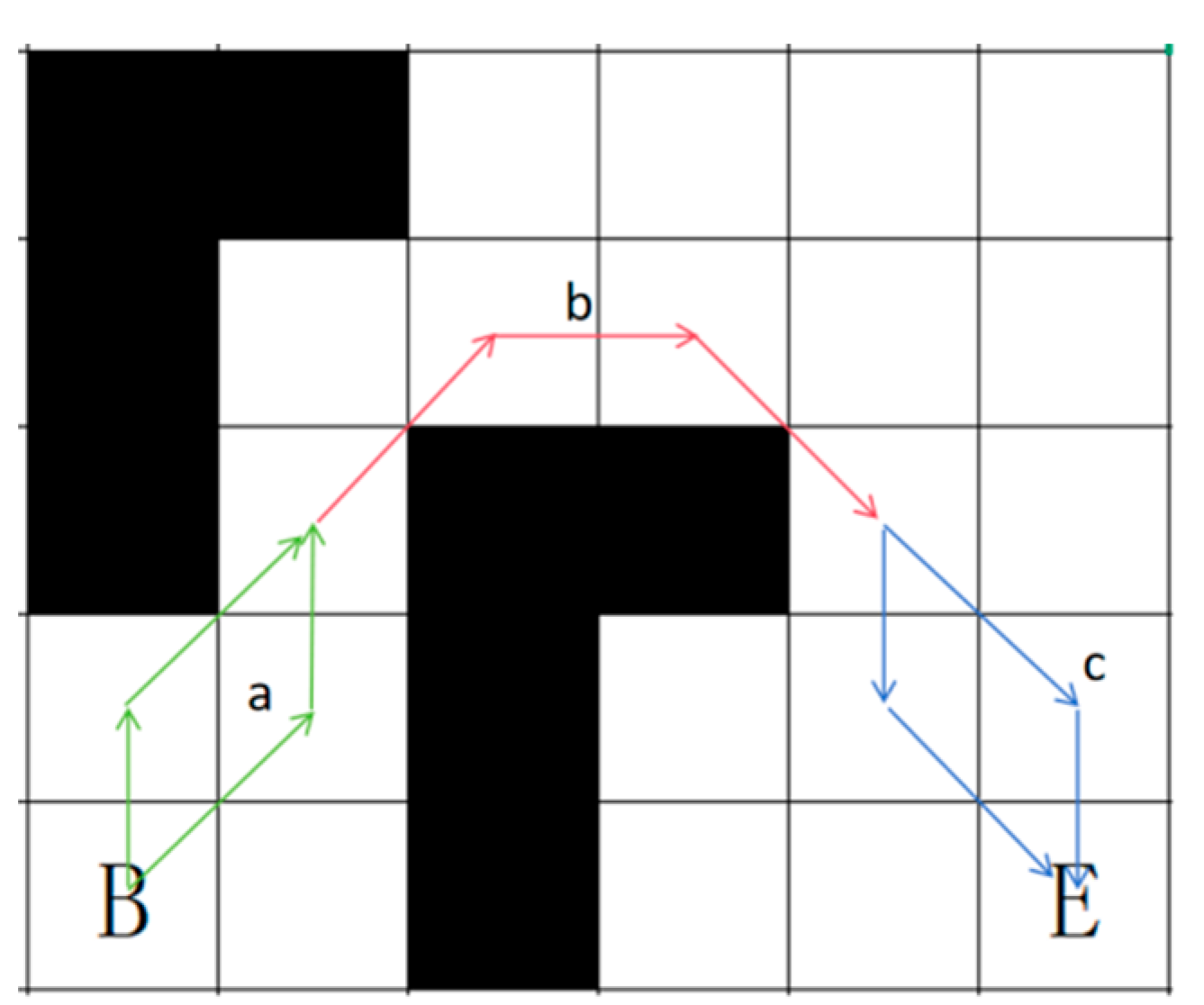
Figure 6.
Axial-oblique movement to construct equivalent path search obstacle vertices.
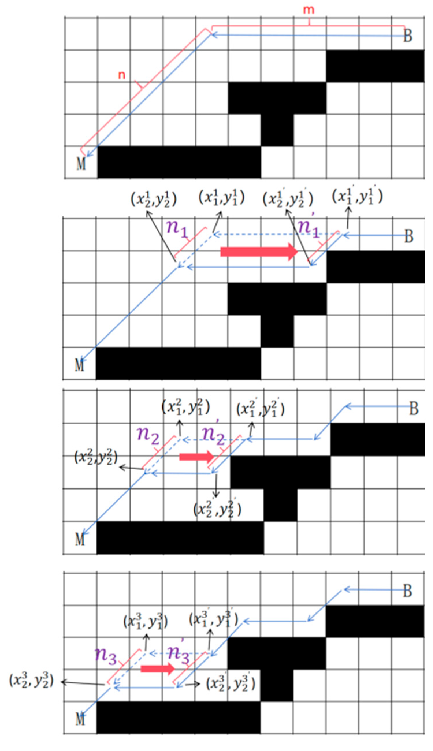
Figure 9.
An example of the path smoothing method.
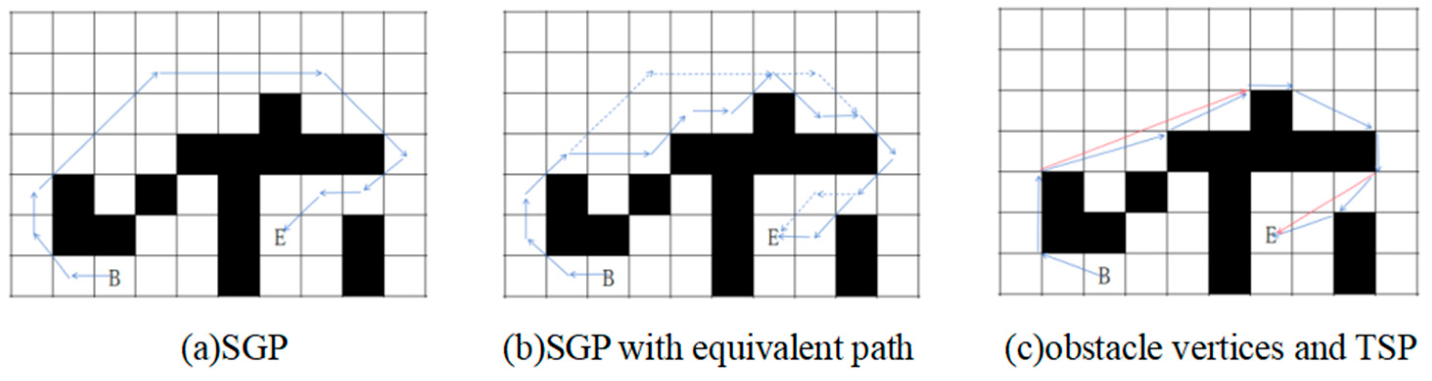
Figure 10.
The data structure for a set of candidate points of length n.
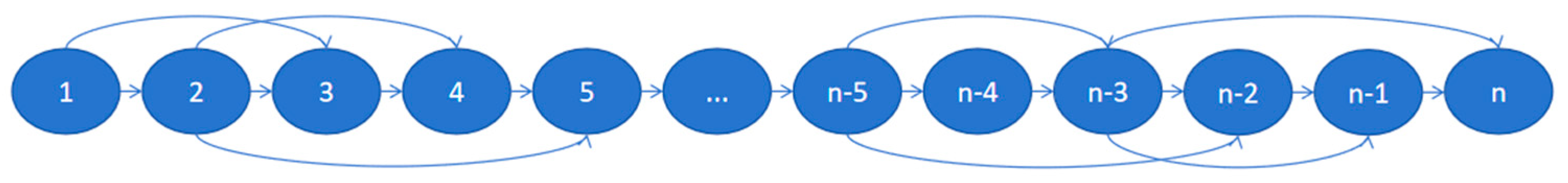
Figure 11.
Replace the path array with an index array.
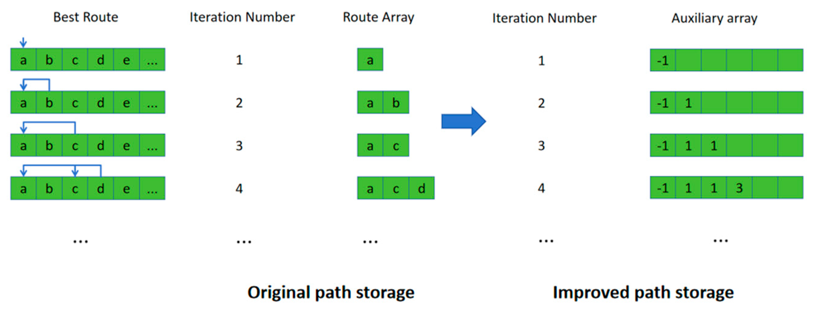
Figure 12.
The adjacent points of the points in the candidate set are continuous in the set.
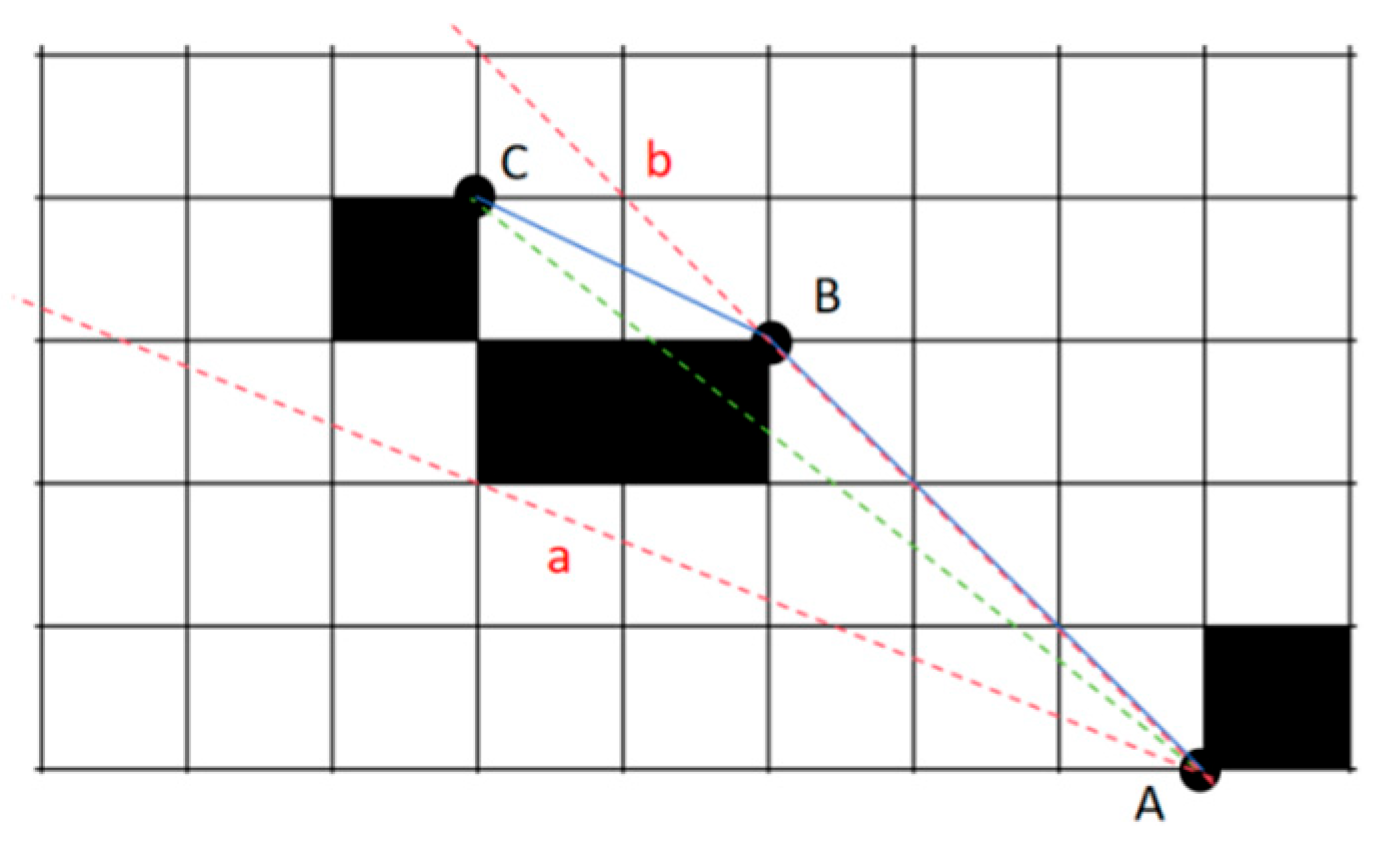
Figure 13.
Flowchart of improved dynamic programming algorithm.
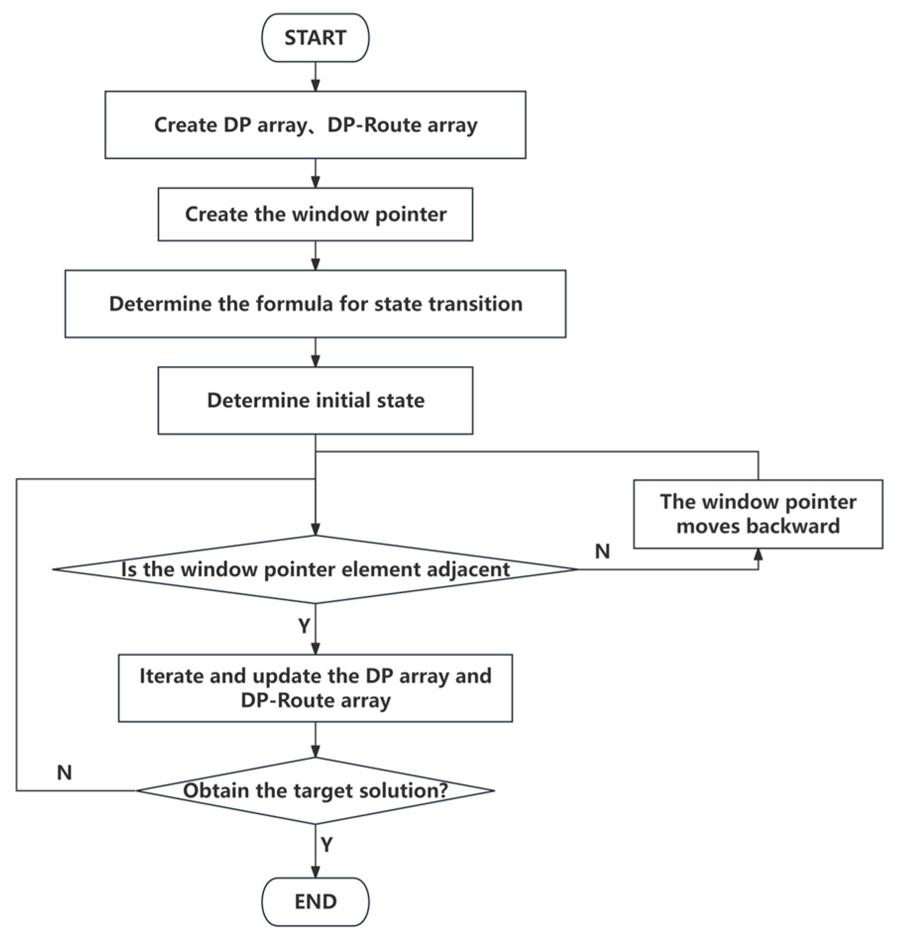
Figure 14.
Comparison of the path length of each part of the ablation experiment.
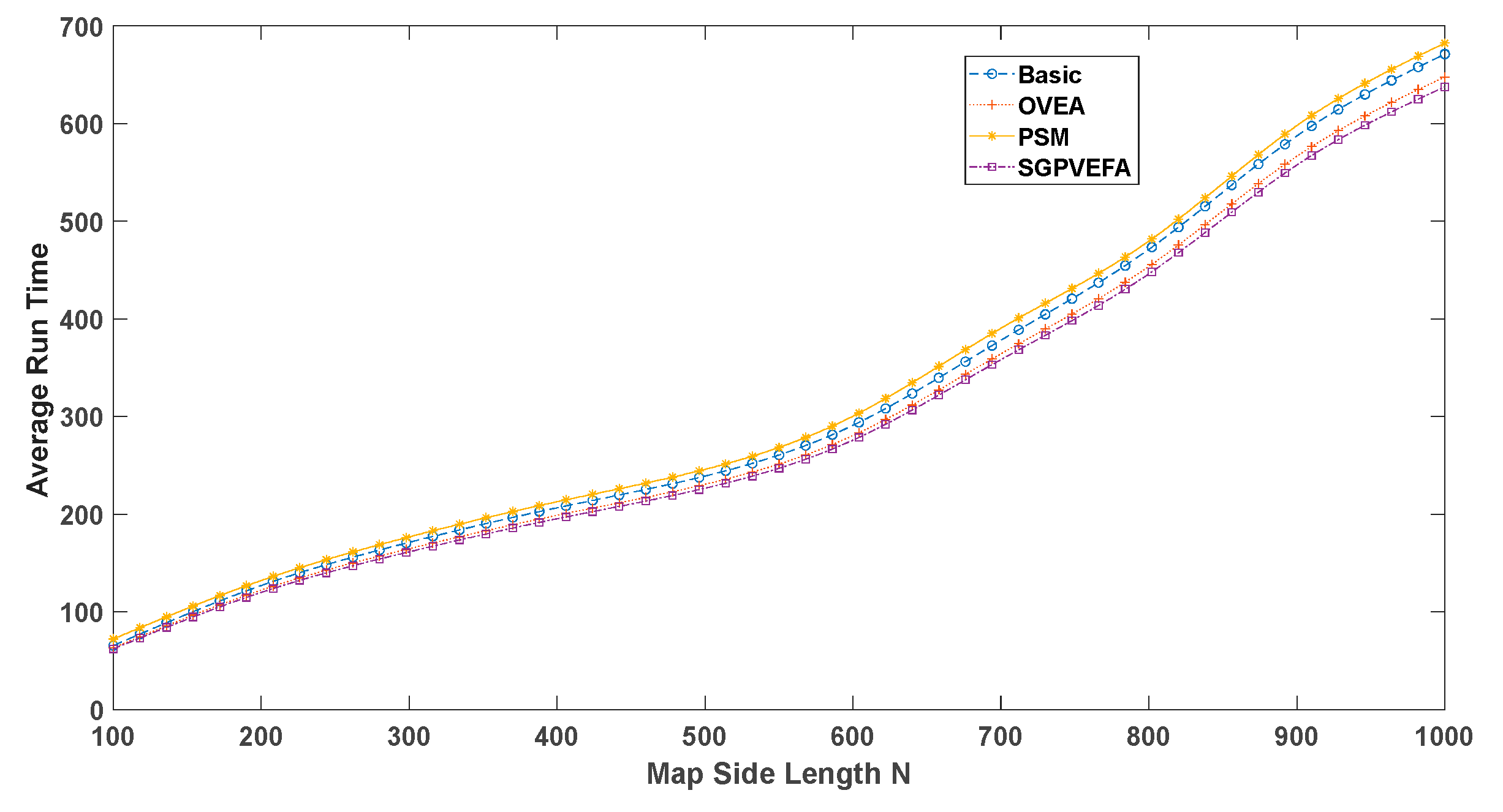
Figure 15.
Comparison of the search time in each part of the ablation experiment.
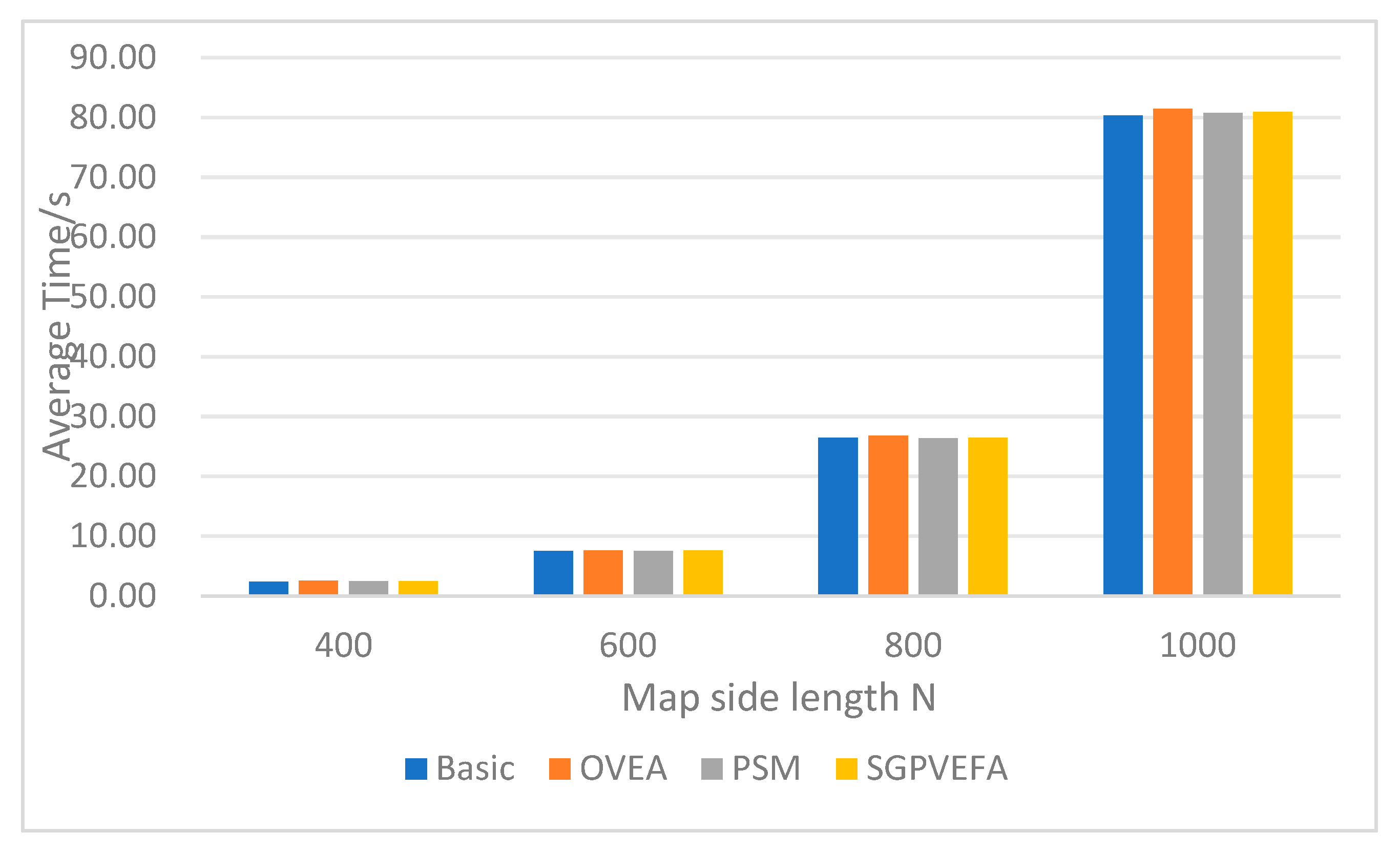
Figure 16.
Comparison experiment of intelligent path planning algorithm (path length).
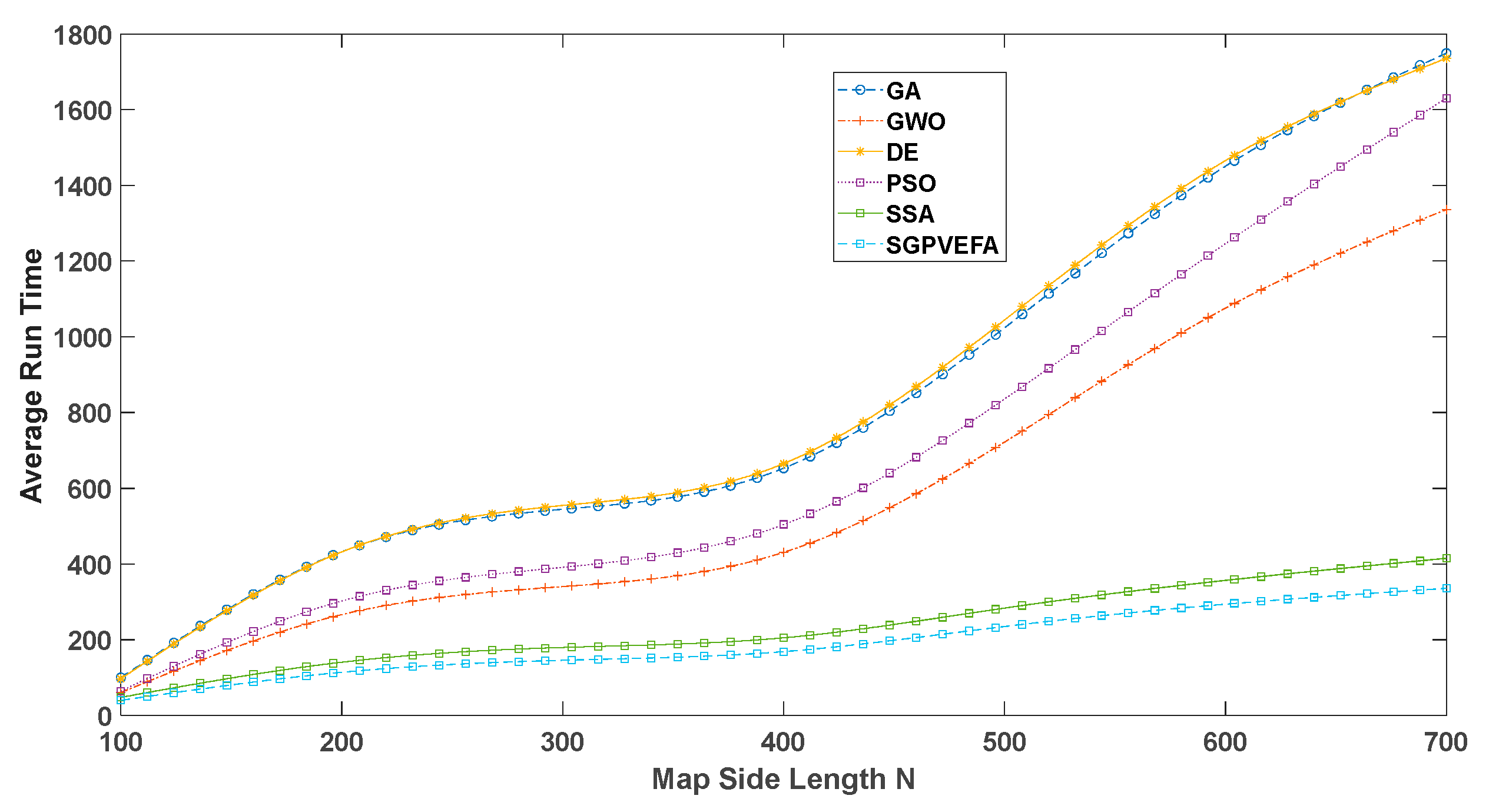
Figure 17.
Comparison experiment of intelligent path planning algorithm (search time).
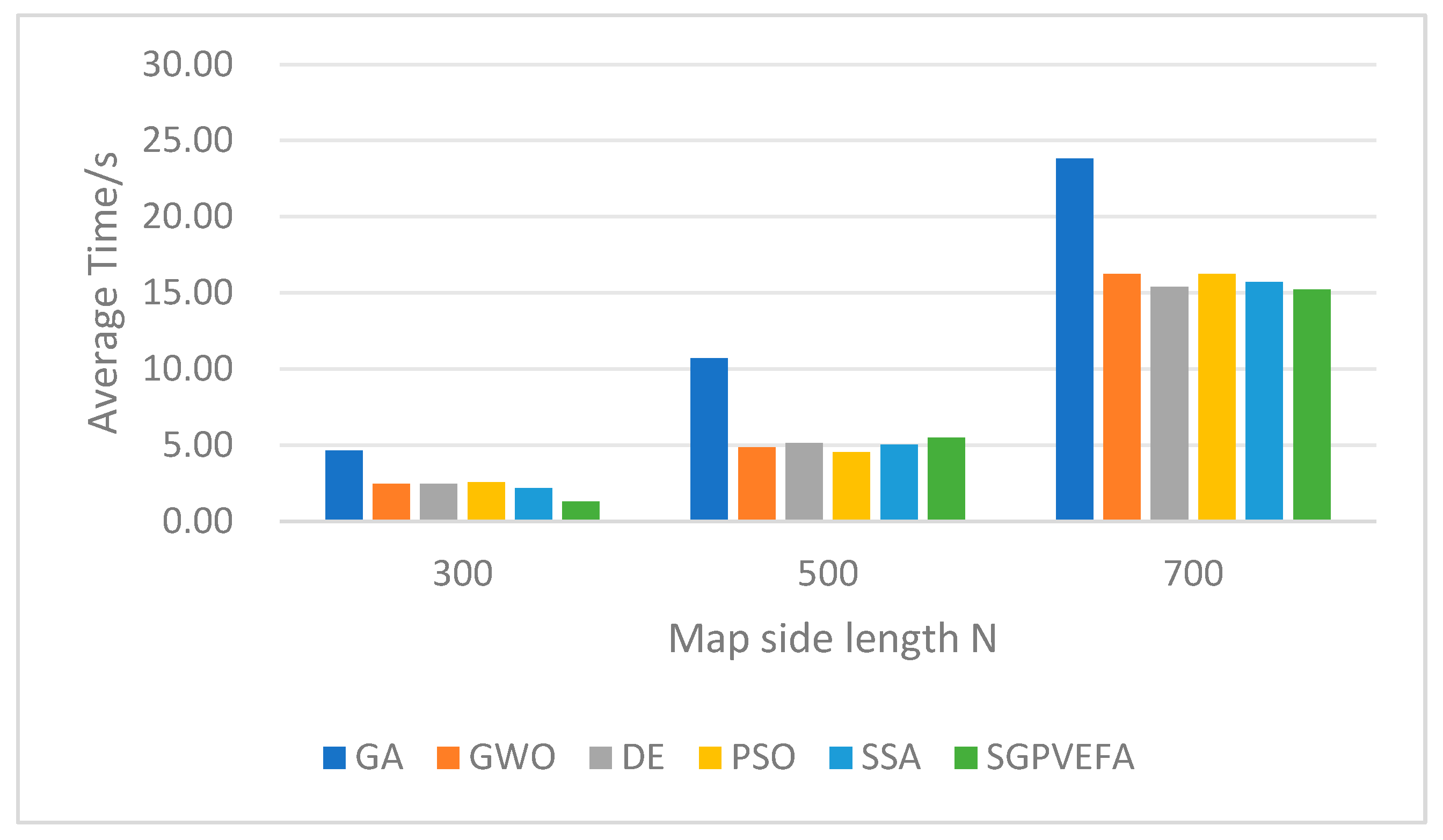
Figure 18.
Path comparison in different environments.
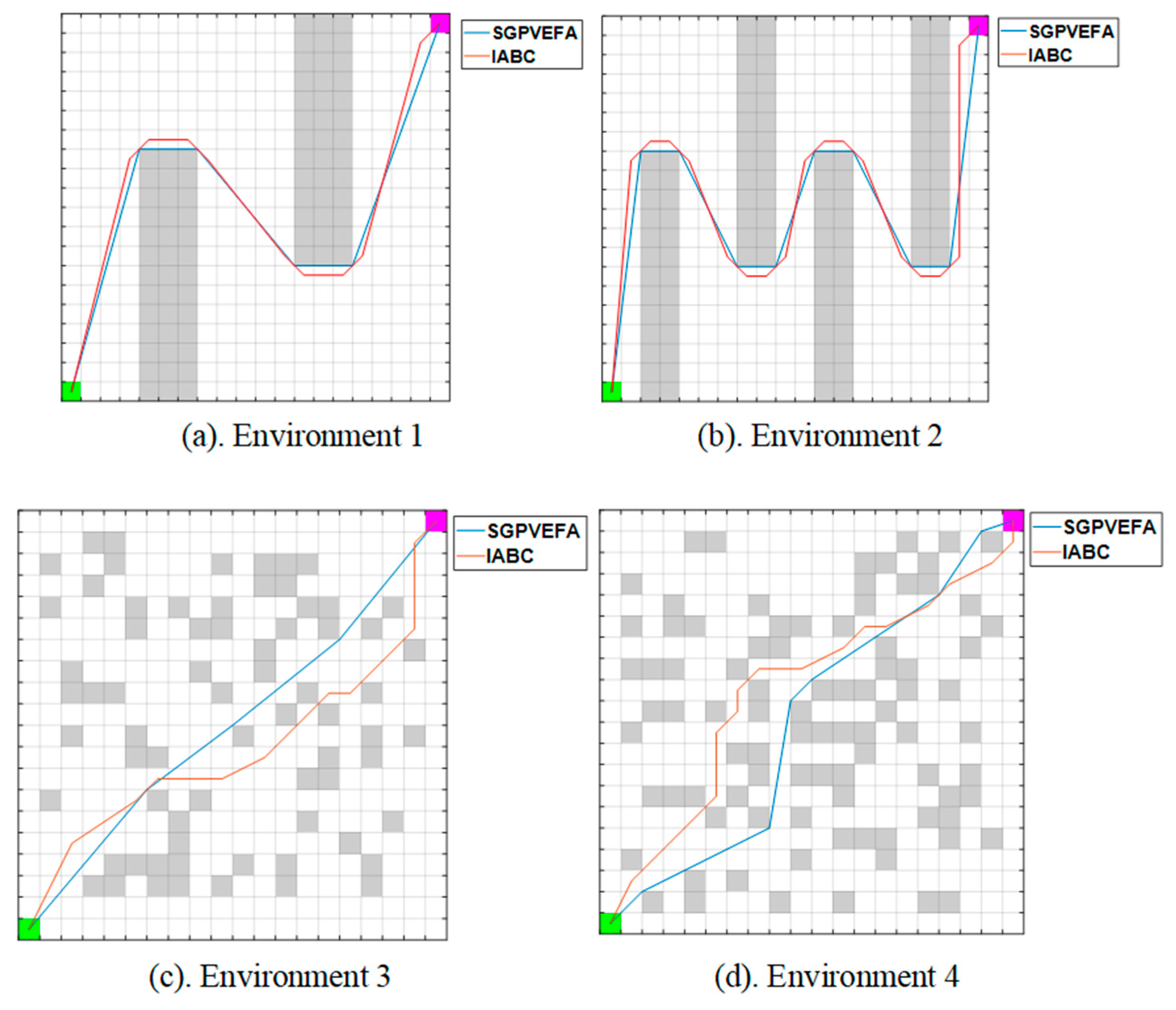
Figure 19.
Comparison of paths found in complex environments.
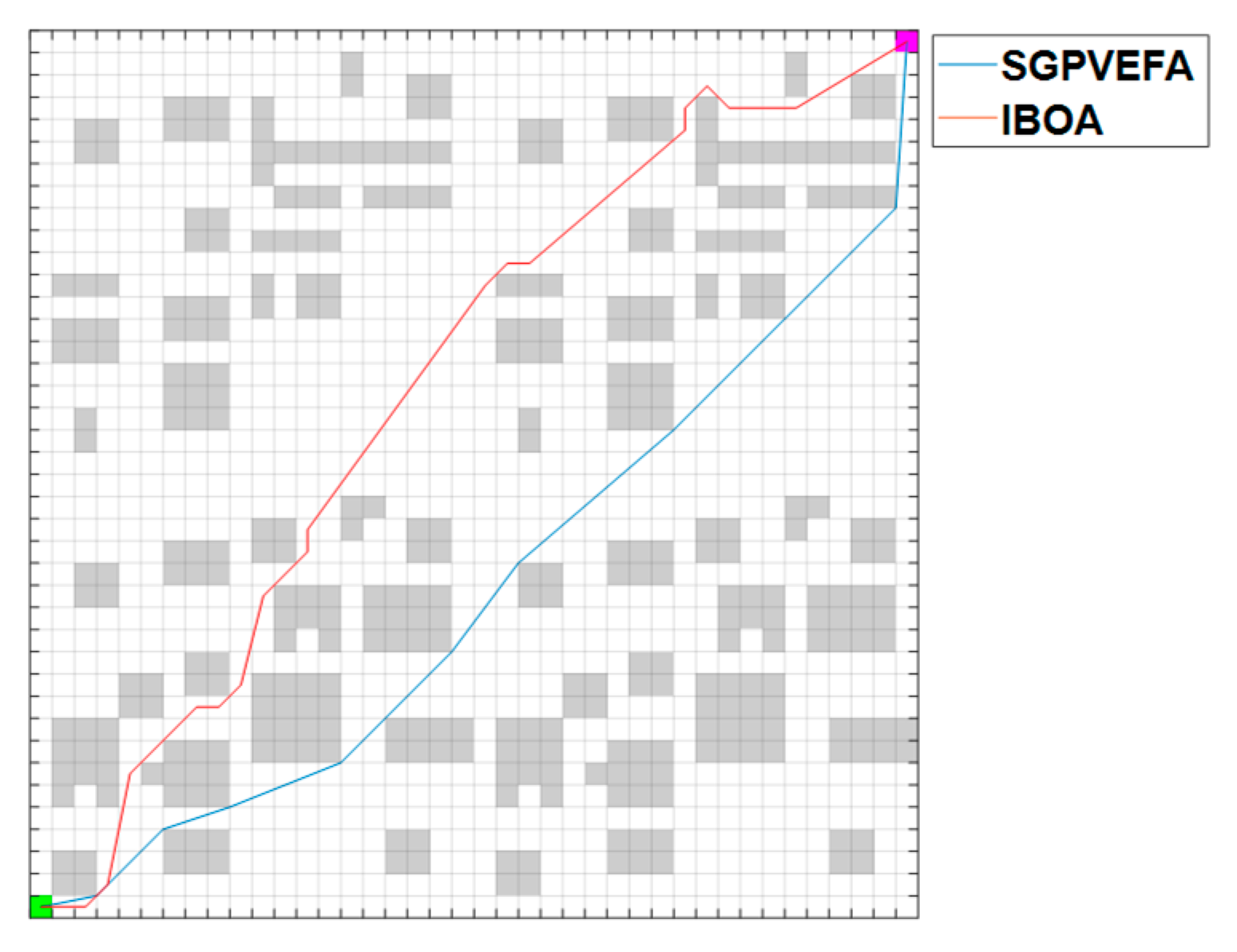

Table 1.
Success rate of each algorithm.
| Algorithm | SGPVEFA | GA | GWO | DE | PSO | SSA | |
| Obstacle rate | Number of run | 50 | 50 | 50 | 50 | 50 | 50 |
| 0.1 | success | 50 | 14 | 32 | 32 | 32 | 31 |
| success rate | 100% | 28% | 64% | 64% | 64% | 62% | |
| 0.2 | success | 50 | 7 | 19 | 19 | 19 | 19 |
| success rate | 100% | 14% | 38% | 38% | 38% | 38% | |
| 0.3 | success | 50 | 1 | 4 | 4 | 4 | 4 |
| success rate | 100% | 2% | 8% | 8% | 8% | 8% |
Table 2.
Comparison of path length and search time with GA.
| Obstacle rate | Algorithm | SGPVEFA | GA |
| 0.1 | path length | 161.41 | 644.60 |
| search time | 4.06 | 6.84 | |
| 0.2 | path length | 185.40 | 485.63 |
| search time | 4.62 | 26.45 | |
| 0.3 | path length | 93.26 | 186.40 |
| search time | 0.78 | 4.79 |
Table 3.
Comparison of path length and search time with GWO.
| Obstacle rate | Algorithm | SGPVEFA | GWO |
| 0.1 | path length | 219.25 | 654.27 |
| search time | 5.56 | 13.85 | |
| 0.2 | path length | 213.83 | 460.11 |
| search time | 4.51 | 25.64 | |
| 0.3 | path length | 88.86 | 124.99 |
| search time | 1.13 | 2.12 |
Table 4.
Comparison of path length and search time with DE.
| Obstacle rate | Algorithm | SGPVEFA | DE |
| 0.1 | path length | 219.25 | 929.55 |
| search time | 5.56 | 13.75 | |
| 0.2 | path length | 213.83 | 584.79 |
| search time | 4.51 | 25.04 | |
| 0.3 | path length | 88.86 | 168.09 |
| search time | 1.13 | 1.86 |
Table 5.
Comparison of path length and search time with PSO.
| Obstacle rate | Algorithm | SGPVEFA | PSO |
| 0.1 | path length | 219.25 | 791.47 |
| search time | 5.56 | 13.49 | |
| 0.2 | path length | 213.83 | 541.41 |
| search time | 4.51 | 27.00 | |
| 0.3 | path length | 88.86 | 119.89 |
| search time | 1.13 | 1.53 |
Table 6.
Comparison of path length and search time with SSA.
| Obstacle rate | Algorithm | SGPVEFA | SSA |
| 0.1 | path length | 218.26 | 281.26 |
| search time | 5.44 | 13.74 | |
| 0.2 | path length | 213.83 | 257.25 |
| search time | 4.51 | 27.31 | |
| 0.3 | path length | 88.86 | 102.09 |
| search time | 1.13 | 1.77 |
Table 7.
Comparison of path length and number of nodes with IABC.
| environment | algorithm | path length | Number of nodes | ||||
| 1 | SGPVEFA | 40.076 | 6 | ||||
| IABC | Best | Mean | Std. | Best | Mean | Std. | |
| 41.245 | 41.245 | 0 | 11 | 11 | 0 | ||
| 2 | SGPVEFA | 52.92 | 10 | ||||
| IABC | Best | Mean | Std. | Best | Mean | Std. | |
| 55.639 | 55.714 | 0.3246 | 18 | 18.933 | 0.2537 | ||
| 3 | SGPVEFA | 27.024 | 5 | ||||
| IABC | Best | Mean | Std. | Best | Mean | Std. | |
| 27.462 | 28.795 | 0.9889 | 8 | 10.4 | 1.6316 | ||
| 4 | SGPVEFA | 28.724 | 9 | ||||
| IABC | Best | Mean | Std. | Best | Mean | Std. | |
| 28.501 | 29.614 | 0.4733 | 12 | 15.033 | 1.2726 | ||
Table 8.
Comparison of path length and number of nodes with IBOA.
| Algorithm | Path length | Number of nodes |
| SGPVEFA | 58.289 | 10 |
| IBOA | 61.016 | 19 |
Disclaimer/Publisher’s Note: The statements, opinions and data contained in all publications are solely those of the individual author(s) and contributor(s) and not of MDPI and/or the editor(s). MDPI and/or the editor(s) disclaim responsibility for any injury to people or property resulting from any ideas, methods, instructions or products referred to in the content. |
© 2025 by the authors. Licensee MDPI, Basel, Switzerland. This article is an open access article distributed under the terms and conditions of the Creative Commons Attribution (CC BY) license (http://creativecommons.org/licenses/by/4.0/).
Copyright: This open access article is published under a Creative Commons CC BY 4.0 license, which permit the free download, distribution, and reuse, provided that the author and preprint are cited in any reuse.


