
Submitted:
15 April 2025
Posted:
16 April 2025
You are already at the latest version
Abstract
A new multi-robot path planning algorithm (MRPPA) for 2D static environments is developed and evaluated. It combines a roadmap method, utilising the visibility graph (VG), with the algebraic connectivity (second smallest eigenvalue (λ2)) of the graph’s Laplacian and Dijkstra's algorithm. The paths depend on the planning order, i.e., they are in sequence path-by-path, based on the measured values of algebraic connectivity of the graph’s Laplacian and the determined weights functions. Algebraic connectivity maintains robust communication between the robots during their movements while avoiding collision. The algorithm efficiently balanced connectivity maintenance and path length minimisation thus improving the performance of path finding. It produced solutions with optimal paths, i.e., the shortest and safest route. The devised MRPPA significantly improved path length efficiency across different configurations. The results demonstrated a highly efficient and robust solution for multi-robot systems requiring both optimal path planning and reliable connectivity, making it well-suited in scenarios where communication between robots is necessary. Simulation results demonstrated the performance of the proposed algorithm in balancing the path optimality and network connectivity across multiple static environments with varying complexities. The algorithm is suitable for identifying optimal and complete collision-free paths. The results illustrated the algorithm's effectiveness, computational efficiency, and adaptability.
Keywords:
multi-robot path planning algorithm
; robotic graph algorithms
; robotic path finding
; robotic collision avoidance
; graph theory
1. Introduction
Motion planning is commonly encountered in environments where several robots operate simultaneously and with multiple obstacles. Motion planning collision-free paths is an important field of robotics, enabling coordinated and efficient operations in various real-world applications [1]. It is also widely used in industrial automation and search and rescue operations such as exploration, object transport, and target tracking [2,3]. A key challenge in motion planning problems is determining an efficient path from an initial location of each robot to the required destination while maintaining connectivity by balancing path optimality and computational efficiency [3,4]. Motion planning is a requirement for ensuring safe and efficient movement of the robots to complete their allotted tasks [5]. Motion planning considers the obstacles in the operational environment and the movements of robots in the environment. Several approaches exist for robots’ navigation, however path planning for multiple robots introduces several challenges, e.g., avoidance of collision and maintaining communication [6,7]. The existing methods, such as potential fields, cell decomposition, and roadmap techniques often do not address these challenges simultaneously. The choice of motion planning depends on the environment and the capabilities of robots. Graph models are more appropriate for robot path and motion planning problems as they provide an intuitive, computationally effective approach to map and navigate the environment. The environment is a configuration space where robots and obstacles are located [8,9].
Graph models are foundational in multi-robot motion planning where the vertices represent specific locations or points of interest in the operational environment and the edges represent the paths or connections between these locations. Thes graph structure allows the planners to use algorithms to determine the shortest or most efficient route between feasible points for the robots to travel [8,9]. Different roadmaps were suggested to achieve this operation, e.g., visibility graphs (VGs) and Voronoi diagrams (VD) [10]. A more popular method used in motion planning problems diagram comprises of Voronoi cells, each associated with a specific site. The edges are equidistant from two or more sites, forming cell boundaries. The cells are entirely convex polygons in 2D and partition space, with no gaps. Voronoi edges are not necessarily straight paths but represent boundaries of the regions based on proximity. Also, VD paths are as far away as possible from the obstacles [10,11,12,13]. Although VD generates long paths that are far from the obstacles (this makes it relatively safe, i.e., collision avoidance due to an increased distance between obstacles and robots, the paths are not optimal [10,11,12]. VG is also a popular method for robot path planning in environments with obstacles. It comprises of vertices and edges representing direct lines of sight between the points. The nodes typically include the obstacles’ vertices, start and end points of the robots’ paths. The edges are straight lines connecting visible nodes, with associated weights often representing the Euclidean distances. An advantage of using a VG for motion planning is its well-understood and straightforward method that produces optimal paths in a two or three-dimensional workspace [9]. It is also computationally effective and guarantees an optimal path when one exist [10,11]. In contrast to the Voronoi diagram, VG guarantees an optimal path; therefore, this study focused on the VG in 2D environments [10,11,12]. This work proposes and evaluates a hybrid approach to solving the multi-robot motion planning problem. It combines VG for path planning, the Dijkstra’s algorithm for optimal path finding, and algebraic connectivity to address path optimisation and maintaining robust communication. The approach is highly suitable for static 2D environments, as the layout is predefined, and the robots need to coordinate their navigation to avoid collisions and stay connected. The traditional path-planning methods often focus on optimising path lengths but neglect the significance of maintaining communication that is critical for cooperative missions.
The Dijkstra’s and A* algorithms were widely used to find the shortest path, but they differ in how they approach the problem and their efficiency in various scenarios [14,15]. In a weighted graph, the A* algorithm aims to find the shortest path between a starting node and a target node with heuristics, especially in environments where a goal is defined. The choice of the heuristic function is crucial. It must be admissible, meaning it never overestimates the actual cost to reach the goal, ensuring that A* finds an optimal path. However, its data storage requirement can be high, as it stores details of all generated nodes, which can be a limitation for large-scale problems. The heuristic method uses assumptions to minimise the complexity of pathfinding. This is a limitation as it requires multiple variables and coefficients which the algorithm designer must select. Also, a well-defined manner for determining these variables has not been previously reported. As a result, the heuristic methods do not provide general solutions. In other cases, the variables of a heuristic algorithm might need modification [16]. The A* search algorithm was not considered in this study because when it is combined with the VG method, the resultant path might not be optimal. It is challenging to compute the heuristic of A*, where the heuristic value is typically a computation of what the straight-line distance to the target would be, if there were no obstacles. Therefore, there is not a method to measure the cost of the straight lines that connects vertices to the goals in an environment where the lines pass through the obstacles. Also, if the heuristic cost is not acceptable, i.e., higher than the actual cost, the identified path may not be optimal regarding the path length [10,11,13]. Therefore, the VG and the Dijkstra’s algorithm are chosen for path planning in this study. Accordingly, a multi-robot motion planning problem becomes the problem of finding the optimal (i.e., the safest and shortest) paths. Furthermore, the VG method can help the robots in the system to move to the desired goal (g) location while avoiding collisions [10]. To integrate algebraic connectivity into this method for multi-robot motion planning, cooperation among robots is optimised by considering the graph’s connectivity that represents their paths. The algebraic connectivity is the second-smallest eigenvalue (λ2) of the Laplacian matrix of a graph that reflects the extent of a graph’s connectivity. A large value for λ2 implies a more robust and a well-connected graph that benefits coordination in multi-robot systems [9].
In this study, the operating environment was a 2D space with polygonal obstacles accommodating multiple robots, each with a start location and a goal position. The aim was to find collision-free paths for the robots as they moved to their respective goals while maintaining a high level of connectivity. This goal was achieved by considering the algebraic connectivity of each robot’s communication graph. The paths in the vector environment model can be represented by the VG [5,8] which has been effective in many applications because of its simplicity, visualisation, and completeness [8]. VG used for multi-robot path motion planning is described as an undirected weighted graph ,where V is the set of vertices representing the robots configurations, the starting and the endpoints of the robot’s movement, is a set of edges representing the paths between the vertices. In the expression , the symbol × denotes the Cartesian product of the set with itself. The Cartesian product V×V is defined as the set of all ordered pairs () where both and are elements of V. Formally, this is expressed as: . In graph theory, this indicates that E, the set of edges, is a subset of all possible ordered pairs of vertices from V. Each edge () in E represents a connection from the vertex to vertex . This framework is fundamental in defining the structure of directed graphs, where the direction of the edge is significant. is a function that assigns the weights (i.e., the path length) to each edge in E. Depending on the context, these weights can represent various attributes, such as distances. The edges denote the physical distance between two points, essential in applications like GPS navigation and logistics. The weights may represent the cost or resource requirements associated with traversing an edge, aiding in optimizing routes to minimize cost. Capacities indicate the maximum flow between the nodes, which is crucial in network design and traffic management. This notation is valuable in problems involving weighted graphs, like finding the shortest path [6,8,17,18]. Edges join all pairs of mutually visible nodes and the edges of the obstacles [18]. Edges exist between two vertices when there is a direct line of sight between them, meaning that the line connecting the vertices does not intersect any obstacle. VG provides a representation of the environment that helps identify robot obstacle-free paths [19]. The weights of an edge represent the Euclidean distances between vertices [20]. Hence, based on the problem’s requirements, it is essential that the VG covers connectivity effectively to avoid a collision and calculates the best path (i.e., the shortest and safest) for the robots [21,22]. Connectivity is critical for a multi-robot team to coordinate and execute complex missions efficiently [9,23]. Algebraic connectivity ensures that the multi-robot system remains well-connected during motions, facilitating communication and coordination. The Dijkstra’s algorithm finds each robot’s shortest path while respecting the connectivity constraints. This optimisation balances between minimising the path lengths with maintaining robust communication among robots [9,23].
This study's contributions include a novel integration of the VG and algebraic connectivity, a communication-path optimisation strategy using Dijkstra’s algorithm, and an evaluation of the proposed methods in static 2D environments. The contributions also include a new path adjustment method based on algebraic connectivity for maintaining strong communication while optimising path lengths (i.e., an optimisation framework that balances path length and network robustness), which addresses the limitations of previous approaches in connectivity maintenance and path efficiency. Combining VG with algebraic connectivity enhances multi-robot systems by ensuring robust communication and an efficient path planning throughout the mission. Our method simultaneously optimised path length and communication robustness. This made it more promising where communication between robots is critical, especially in cooperative tasks. Connectivity indicates a more resilient network capable of withstanding individual robot failures without losing overall connectivity. Therefore, enhancing algebraic connectivity strengthens the communication network, ensuring the robots remain connected during operations. In the following sections, the related theory is explained, the study’s methodology is described, and the results are discussed.
2. Related Theory
In this section the theoretical concepts related to the study are explained.
2.1. Overview of Multirobot Path Planning Algorithms
Considering a multi-robot environment which has a limited finite communication range (R) and is modelled as an undirected weighted graph the following are defined:
- is the set of vertices representing the n robots,
- is the set of edges representing paths between vertices, where ,, exists between vertices, if robot n interacts with robot m; this means two robots can communicate only if they are within the communication distance of each other, also the presence of the edge refers to the presence of the edge. Therefore =, signifies that the edge is mutual and directionless. This characteristic is fundamental to undirected graphs, where edges do not have a specific direction.
- is function that assigns the weight (length path) to each edge in E. is a set of weights so that and otherwise.
If we consider a team of n robots, the set of neighbors of the ith robot can be defined as , all robots that can communicate with it. Hence, each robot is assumed to be able to interchange data with its neighbors [9,23,24]. A method to represent such an undirected weighted graph is using the Laplacian graph and its algebraic connectivity as an indicator of the system’s connectivity. The algebraic connectivity is defined as the second smallest eigenvalue ) of the graph Laplacian. Let the graph Laplacian be the weighted matrix which combines the adjacency (A) and the degree matrix (D). Here is the weight function, which can be seen as a function of the distance between robots i and j. is called the algebraic connectivity value of the system. The value of the algebraic connectivity differs from zero (= 0) if the graph has disconnected components, i.e., no paths among vertices or two disconnected components [25,26]. If is very small, it refers to the graph being nearly disconnected. Non-zero connectivity refers to a path among every pair of vertices (robots in the system) in the graph. A higher algebraic connectivity signifies a more robust and well-connected graph with many edges, i.e., the value of ranges between 0 and the number of vertices (N). In addition, connectivity refers to the number of vertices in the graph, if the graph is completely connected. Thus the maximum value of, and it is obtained when the entries of the adjacency matrix are all equal to 1, that means all possible edges are present in it [9,23,24].
2.2. Algebraic Connectivity for Communication of Multi-Robot Systems
The second smallest eigenvalue (is indicated as a constraint to maintain communication during the motion. It ensures the robots remain well-connected for communication or coordination during their tasks. This is critical in scenarios where the robots need to share information or collaborate to perform tasks. The term is a function of the whole system’s state. It is an important parameter that affects the performance and robust properties of dynamical systems working over an information network [24]. Algebraic connectivity maintains connectivity and enables them to execute tasks while maintaining connectivity within the system. Connectivity is managed by strategically adding edges that optimise the network's structure to maintain robust communication within the system. This involves measuring the second smallest eigenvalue of the Laplacian matrix, known as the algebraic connectivity, and iteratively adjusting path calculations to ensure remains high. A higher algebraic connectivity signifies a more resilient network capable of withstanding individual node failures without losing overall connectivity. By focusing on this metric, the system enhances communication robustness while minimising path lengths [24,25,26]. Hence, this enables the robots to obtain complete information about the surroundings of the workspace environment to avoid collision and to find the best safe paths. The weights of the edges control the motion time of robots, where edges’ weights are functions of the inter-robot distances. Consequently, these weights can directly influence the time taken for a robot to move along a particular path. In robotics, motion time refers to the time for a robot to traverse from one location to another within the network. For example, edge weights are determined by inter-robot distances; a greater distance (and thus a higher edge weight) would typically correspond to a longer motion time for robots. This relationship is crucial in optimising robots’ trajectories to ensure efficient movement and coordination within the system, and it is essential for effective motion planning and coordination in multi-robot systems [9,23].
In a workspace environment, we have assumed that the obstacles were convex, static and that the distance between any two obstacles was greater than the size of robots. We considered two types of collisions: (i) collision between an obstacle and a robot and (ii) inter-robot collisions (i.e., collision between two robots). Each robot could determine the presence of an obstacle and measure its relative location and the distance from its boundary within the communication range. Therefore, the aim was to solve the problem of a team of multi-robots, which began from the first configuration where the team was connected ( > 0), maintaining connectivity whilst being controlled to achieve a desirable objective to avoid collision until reaching the target configuration. A collision avoidance mechanism was executed that prevented robots from colliding with each other. Their communication was defined based on the weights of the edges (which determined the quality of the communication links between the robots), and when was non-zero, whilst every robot tracked its paths to reach its goal location [9,23,24]. In addition, during the path planning, the weights () of the vertices changed and became equal to the moments at which the robot () passed through these vertices [8]. Therefore,
2.3. Collision Avoidance
To provide collision avoidance, the weights of the edges can be modified during path planning, either by path correction, where a robot is not allowed to move on the edge that is occupied by another robot, or through controlling the robot’s motion time on some edges by controlling the distances between the vertices to free up the paths for other robots, the paths of which are planned earlier [8]. This means the increased time of the robots to traverse the graph edge from vertex . So, we have two principal conditions that need consideration for path correction and control robot motion time to avoid a collision. First, two robots cannot cross paths simultaneously on the same vertex of a graph. Thus, if this happens, to prevent collisions, let be the arrival time (i.e., the time when robot passes through the vertex , and be nth robots, (n=1,2,…,p and p represents the number of robots). is expressed as
In the given context, represents the arrival time of robot at vertex . denotes the time at which robot departs from vertex represents the travel time required for robotto move from vertex to vertex . Therefore, the equation suggests that the arrival time at vertex is the sum of the departure time from vertex and the travel time between vertices and This formulation is commonly used in multi-robot path planning and scheduling to ensure coordinated movements and to avoid collision.
We will assume that is a minimum value of safe distance to ensure collision-free motions. Then, must provide a safe passage for the robots when crossing the crossroads through increased weight edge (distance) on the graph from the vertex ( to vertex to increase the motion time of the robot on a graph edge by time units that correspond to its motion time change. By other means, ϵ is a small increment; the unit of which is typically meters, or the relevant unit of distance measurement used within the system. By incorporating ϵ into the edge weights of the graph, the weights are iteratively adjusted to avoid collision between the robots by incrementing ϵ to obtain optimal weights that improve its performance on the given task. This adjustment effectively increases the perceived distance between vertices and , discouraging robots from occupying the same intersection simultaneously and thereby reducing the risk of collisions. Therefore is a safety value from which two robots will not collide, the weight of vertex is calculated according to Equation 1. Second, it is not permissible for any two robots to move together on the same edge in opposite directions. Therefore, if any two robots are moving in opposite directions on the graph edge (straight paths) at the same time, then
then
Given mth robot () and nth robot (), part in Equation 3 implies that two conditions need to be satisfied simultaneously (the symbol ^ denotes the “AND" operation). These conditions compare weights , and the arrival times of . The > part in Equation 3 implies that the time for , i.e., must be greater than the time for , i.e., , because of the previous conditions. No collision occurs as passes through the edge before , whose path is being planned and drives onto the edge. Hence, in this case, the edge weight does not require changing. Then, the vertex weight is calculated as Equation 1. depends on the distance = between the edges of the graph. If this means the distance travelled by is less than the distance travelled by , hence the arrival time of is greater than the arrival time of [8]. On the other hand, if
Then, the vertex weight is defined as Equation 1. In addition, if
then (6)
This occurs when two robots move in opposite directions, and whose path is being planned crosses through the edge before , no collision will occur; thus, the weight of edge does not need to change. The weight of the next vertex is calculated as Equation 1. In contrast, if
^ (7)
A collision is possible when the robot follows the robot, which its path is being planned, and collides with it on the edge [8]. To avoid a collision, it is essential to modify the edge weight of the current robot (i.e., changing the arrival time through increasing distance) according to Equation 5, and then the vertex weight is defined as Equation 1. Also, if
then (8)
Then the collision is possible when follows and collides with , which its path is being planned before the crossroads [8]. To avoid a collision, the arrival time of the current robot must be increased. So, the edge weight must be changed based on Equation 5, and then the vertex weight is calculated as Equation 1.
3. Materials and Methods
In this section the procedures followed to obtain the results are described.
3.1. Operation of Mult-Robot Path Planning Algorithm (MRPPA)
To address the motion planning problem for a multi-robot system and to find a collision-free optimal path, the algorithm based on the VG method is proposed. The algorithm consists of the main tasks (i)-(vi):
- Establish a free workspace map.
- The algorithm defines each robot’s starting position () and goal positions () and the number and locations of obstacles.
- All obstacles in the map are modelled as polygons to facilitate efficient and accurate pathfinding. A polygon also allows creation of visibility graphs where the vertices represent the obstacle corners, and the edges denote direct lines of sight between them. This framework is essential for determining the shortest collision-free paths. Polygonal obstacle modelling aids in expanding the obstacles appropriately to account for the robot's size. This process ensures that path planning algorithms consider the robot's physical footprint, preventing collisions. Also, robotic systems can effectively navigate complex environments, ensuring accurate and efficient movement, while avoiding collisions. The algorithm analyses the position of each obstacle’s vertices. The robots’ starts and goals positions are known relative to the obstacles in the surrounding environment. Each robot is considered a dynamic obstacle.
- Using the constructed free space and VG algorithm, the robots can navigate without colliding with the obstacles.
- The workspace environment is divided into two disconnected components of undirected weighted graphs. Then, the best edges are chosen to add between these two graph components to find the paths for each robot, based on the measured values of algebraic connectivity of graph Laplacian, which controls the inter-robot connectivity when it is unequal to zero.
-
When planning a path for a robot, its vertex weight is changed just as in the single-robot path planning algorithm. The weights of the vertices of the graph are initialised with the maximum possible value, i.e., infinity (∞), whilst the start time value initialises the start vertex ( = ). According to the known edge weights, the Dijkstra’s algorithm is applied to find the shortest path based on the cost corresponding to each edge (distance between vertices), where the shortest path is the path with the minimum length. Therefore, it is required to find a vertex sequence (series waypoints), which denotes the shortest path from the starting point to the goal point. If the Dijkstra’s algorithm finds the shortest paths, the robot’s path can be changed based on the distance, corresponding to the environment model correction. The MRPPA algorithm is described as:Inputs: Start positions (), goal positions (), polygonal obstacles ().Outputs: Visibility graph (VG), Optimal paths from start ) to goal ().
- Establish a free workspace map.
- Determine each robot’s start and goal positions and obstacles’ vertices numbers and locations.
- Divide the workspace environment into two disconnected components of undirected weighted graphs .
- Select the best edges (, where i and j represents the edge between two vertices) to add between these two components of the graph based on the measured value of algebraic connectivity of graph Laplacian ().
- Create the visibility graph (VG).
- Find a vertex sequence (series waypoints) from the start () to goal () by using Dijkstra’s algorithm, which denotes the shortest paths.
- End: paths is calculated where start point and = goal point.
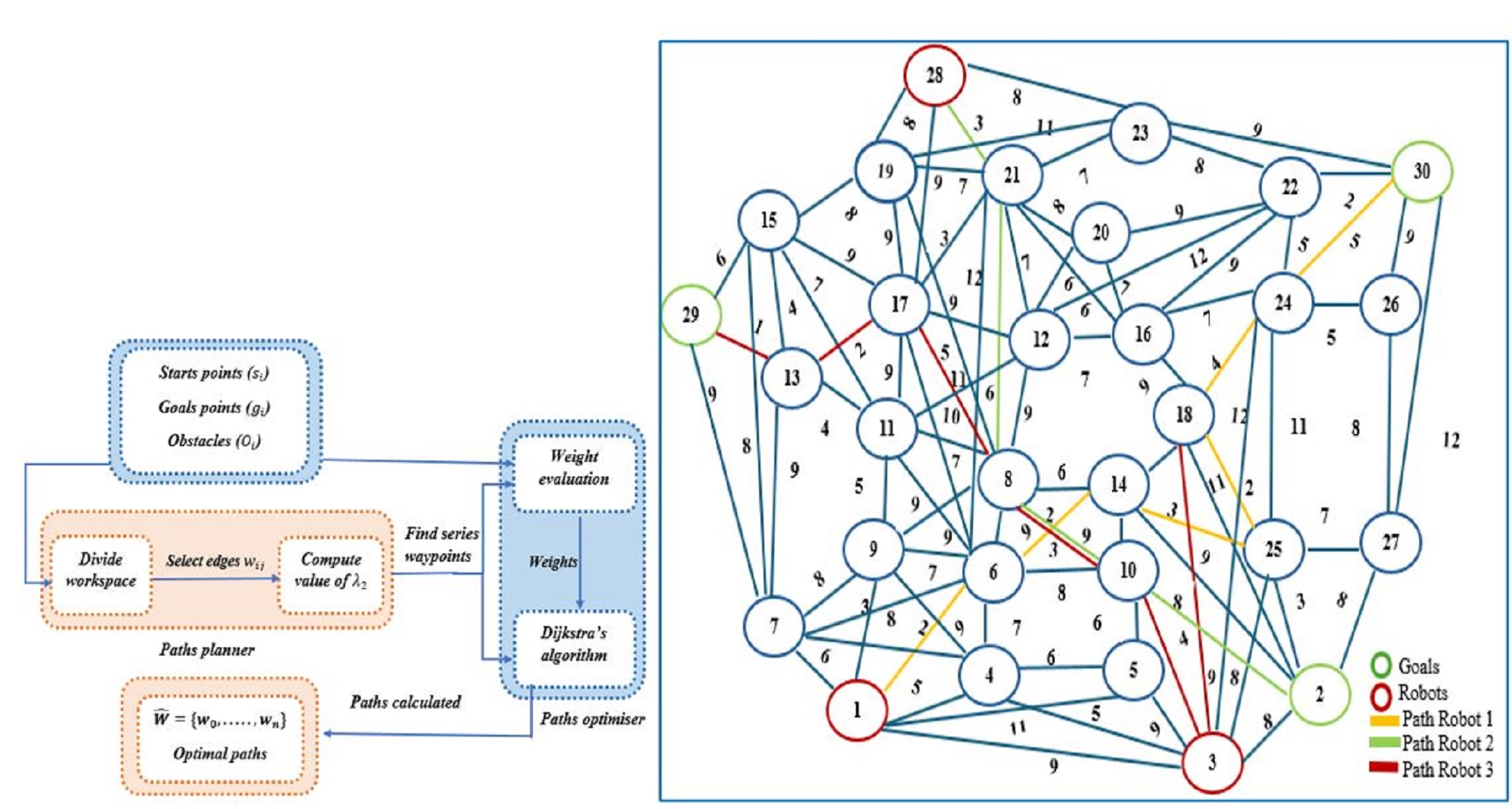
The operations of MPRR algorithm are also illustrated in Figure 1.
The key objective of the MRPP algorithm is to find optimal paths for all robots by minimising the path length. It maintains λ2 of the communication graph at a high level to ensure the multi-robot system remains connected during the motion and provides collision avoidance.
3.2. Procedure to Implement MRPPA
The MRPPA was implemented by following the steps:
- Create VG for the environment, including all the start and goal positions of the robots. Each robot can be represented as a vertex, and edges existing between the robots. The edges (connections) between these vertices refer to the corresponding robots, are within a certain communication range and can directly exchange information.
- Evaluate connectivity by calculating and define the communication or interaction graph between the robots. The Laplacian matrix L of this graph is constructed, and its eigenvalues are determined (). Higher algebraic connectivity implies that the robots are well-connected, meaning the communication graph is robust to disconnection for coordinated motion.
- Carry out an initial path planning by using the Dijkstra’s algorithm to find each robot’s shortest path from start to finish.
3.3. Description of the Optimisation Process
During a motion planning process, the algorithm selects paths for the robots that minimise their travel distance and ensures that each robot network’s algebraic connectivity is improved and maintained [25]. The optimisation process involves calculating the paths and connectivity at each step as outlined by the steps below.
- If is the small, indicating weaker network connectivity, the paths can be adjusted to improve connectivity. Robots’ paths can be altered to keep them within the communication range of others. This may involve adding edges to maximise or maintain a high level of algebraic connectivity, thereby strengthening the network's resilience to disconnections. The objective of adding edges is to increase robot proximity, increase , improve connectivity and to ensure the communication graph remains connected.
- Run the Dijkstra’s algorithm on the visibility graph for each robot to find the shortest initial paths.
- Repeat the above operations until optimal path lengths are obtained for all robots to reach their targets while maintaining communication.
4. Results
The key aim of the optimisation is minimising the path length (the total distance travelled by the robots) while maintaining a minimum level of connectivity in the communication graph. To illustrate how the algorithm operated, a scenario comprising six obstacles was considered as shown in Figure 2. The robots are R1-R3 and associated goals are g1-g3.
The workspace scenario depicted in Figure 2 is represented as an undirected weighted graph in Figure 3. In this figure, the vertices correspond to specific locations or points within the workspace, and the edges represent the possible paths connecting these points. The weights assigned to each edge indicate the cost or distance associated with traversing that path, facilitating the analysis and optimization of movements within the workspace.
In this scenario, there are three robots and three goals. The workspace is divided into two disconnected components of an undirected weighted graph using VG, such as in Figure 4.
The graph in Figure 3 consists of vertices marked from =to and E = {}. There are six polygonal obstacles (, ). Each robot has an initial position () and the goal positionHere, there are three goals for the three robots. The second smallest eigenvalue of the graph in Figure 2 has zero value, i.e., (which means the graph is disconnected. The robots (, exist in the first component that contains vertices:, where vertex is a goal for . Subsequently, can find a way to reach its target , but and do not have paths to reach their targets. The second component contains vertices:vertices are goals for and respectively. When an edge was added between the vertices and increased to 0.087, and this enabled R1=v1, to find a path to reach its target ). Whereas if two edges added and), increased to 0.181 which allowed ( to find the most suitable path to reach its target Furthermore, when the three edges were together {} increased to 0.347, and R2 found a path to reach its goal ). When all possible paths were added between the vertices of the graph, the second smallest eigenvalue increased and a robust connectivity was created in the graph, where 6.380. The safe shortest paths are found using Dijkstra’s algorithm, as shown in Figure 5. The shortest paths for three robots using Dijkstra’s algorithm is shown in Figure 6.
The MRPP algorithm planed the path for each robot based on a specific sequence or priority i.e., the first path for , the second path for , and the third (last) path for . There is an intersection (crossroad) between the paths of and , and opposite directions on the graph edges (straight roads) between the paths of and . However, no collision occurred as the algorithm has planned a path for each robot sequentially (one by one). Hence, when planning the following path, it considers all the paths that have already been scheduled to prevent collisions and keep . There is a crossroad when passes the edge and passes the edge, but no collision occurs as passes before . The arrival time of when passed the vertex (is:, and once passed the vertex (:. Whereas the arrival time of once passed the vertex (:, and when passed the vertex (. Consequently, that the arrival time of to the vertex is shorter than the arrival time of to the vertex because the distance (edge weight) that has passed the vertex is less than the distance (edge weight) that has passed the vertex thus when arrives at the vertex (, arrives at the vertex , for this reason, no collision occurs, and a change of the edge weight is not necessary. If, then a collision is possible (i.e. if the arrival time of on the vertex (), then the change of the edge weight is necessary to avoid a collision. Also, there are opposite directions (straight paths) on the edge betweenand . passes the edge earlier than the , whereand . Thus, the arrival time of once it passes the edgeis shorter than the arrival time of as the distance that has passed to arrive at the vertex is less than the distance that has passed the vertex (. Thus, . In addition, there is a crossroad on the vertex (, where , and , hence the arrival time of to the vertex ( before . Accordingly, there is no need to change the edge weight since no collision occurs. If, then the collision happens, so the change of the edge weight is necessary to avoid a collision. These are highlighted in Table 1.
To further illustrate the process, the workspace environment is changed to Figure 7.
To apply the MRPPA, the workspace is represented as an undirected weighted graph, then divide it into two disconnected components of an undirected weighted graph using a VG such as Figure 8.
The graph in Figure 8 consists of vertices, where the vertices represent initial robot positions = that marked with red, while the verticesrepresent goals positions that shown as green, E = {}, and there are five polygonal obstacles (). The second smallest eigenvalue of the graph has zero value (because the graph has two disconnected components. has a path to reach its target, whilst and have their targets in the second components of undirected weighted. If an edge is added between the vertex and vertex, then can find a path to reach its target , and from this increases to 0.521. Also, if we add the edges,), andThis enables to find a path to reach its target, and increases to 1.275. Additionally, when adding all possible edges between the vertices of the graph, we created robust connectivity in the graph, and increases to 2.855. The shortest paths are found using the Dijkstra’s algorithm, as shown in Figure 9 and Figure 10.
The MRPPA planned the first path for R3, the second path for R1, and the third path for R2. No collision occurred because the algorithm has controlled the arrival time of each robot by holding the weight of the edge (distance) and keeping >0.
4.1. Simulation Procedure
This section introduces the simulation setup, parameters, and results of implementing the MRPP algorithm. This algorithm leverages VG for obstacle avoidance, algebraic connectivity to maintain communication cohesion, and Dijkstra’s algorithm for optimal pathfinding.
Simulation Environment: The path planning software simulations were conducted in a MATLAB/Simulink environment version 2024 (The MathWorks, Inc. with the Robotics System Toolbox) [27], leveraging custom VG generation and pathfinding scripts. All required inputs were supplied to perform and complete the path planning process and follow a specific logical order. A 2D environment with static polygonal obstacles was devised, representing a workspace of dimensions (18 × 12) units, where each unit represented one-meter square. The obstacles were defined as geometric shapes such as triangles, rectangles, squares, zigzag lines, etc, and robots were modelled as points.
Parameters: Three robots (R1, R2, R3) appearing as three red points were selected. Three goals (g1, g2, g3) were represented by green points. The six randomly generated polygonal obstacles () of varying sizes were highlighted in blue with different labels. Each robot was initialised at random start points and assigned unique goal positions. The algorithm’s effectiveness was evaluated in different scenarios with varying obstacles and number of robots. The performance metrics included path optimality and connectivity maintenance.
Motion Planning Approach: Each robot computed a visibility graph to represent possible paths around obstacles, connecting vertices (obstacles’ vertices, and start and goal points) with edges representing collision-free paths. Dijkstra’s algorithm was applied to find the shortest route to the goal for each robot. Algebraic connectivity was constantly measured, ensuring all robots remained within the communication range. Adjustments were made to the paths when the connectivity = 0 or very small.
4.2. Results for the Simulation Scenarios
Scenario 1: Six obstacles, three robots marked red, three goals marked green are shown in Figure 11 and Figure 12.
In the first scenario, three robots were deployed highlighted with six obstacles density marked as blue. VG was established, and each robot’s path was computed using Dijkstra’s algorithm. The connectivity was maintained throughout the simulation. All robots successfully reached their goals as illustrated in Figure 13.
The simulation results using MATLAB show that the robots reached their targets, the path of R1 is highlighted as yellow, the path of R2 is highlighted as green, and the path of R3 is highlighted as red as shown in Figure 14.
Scenario 2: Five obstacles, three robots highlighted as blue and three goals highlighted as green, see Figure 15 and Figure 16.
In scenario 2, three robots highlighted in blue, and three goals highlighted in green navigated an environment with obstacles. A VG was generated for each robot. Dijkstra’s algorithm was used to measure the distance for each robot. All robots reached their targets while maintaining connectivity, as shown in Figure 17.
The simulation result (Figure 18) shows that each robot has reached its target without a collision.
5. Discussion
The proposed multi-robot motion planning approach was evaluated through experiments using different environments with randomly placed obstacles and different robot configurations. Robots were assigned random start and goal locations, navigating through environments of varying obstacles. For each configuration, performance metrics included path length and the total distance that each robot travelled, i.e.,
- Computation of path: Calculating paths while maintain connectivity.
- Algebraic connectivity: A measure of communication robustness among robots.
- Success Rate: The robots reaching their targets without collisions or connectivity loss.
These metrics align with the previous studies such as [28], which emphasised path efficiency, robustness, and connectivity in multi-robot systems. The proposed paths contained two main components: a global planner and path optimisation. The global planner gathered information about the surrounding environment, such as the robot’s positions, targets, and obstacles. Depending on the path analysis, finding the path with minimum cost is necessary. When the optimal path is found with prior knowledge of the environment and static obstacles, a collision-free optimal path was created before the robots moved. One finding is that the proposed algorithm significantly improved the generation of efficient paths due to connectivity robustness, and robots reached their goals reliably without collisions.
In tests with three robots for connectivity maintenance, the MRPP effectively determined paths by analysing all possible routes and selecting the most suitable one based on the algebraic connectivity measure and the predefined weight evaluation function, indicating adaptability. The algorithm planned a sequential path for each robot one by one (i.e., path by path), considering all already planned paths to avoid collisions. The MRPP algorithm provided each robot's optimal (i.e., short-distance and safe) paths. The lengths, and motion times of the paths were based on the planning order. The choice of the correct sequence for the path planning of robots has a significant impact on the performance of the robot team. In the first scenario of workspace, has a path to reach its target: ), and the total distance is (20 m), see Figure 4. However, this path is not optimal and ( = 0) meaning the graph is disconnected. Thus, for optimisation, the MRPPA re-calculated the path and examined the two best edges and) to add between the graph components and measured algebraic connectivity. The algorithm found an optimal path for R3 instead of the first path while maintaining of the communication graph at a high level (for R3, . The total distance is (15 m), and ( increases to 0.181), see Figure 5. Accordingly, the MRPPA chooses a path for each robot respectively to ensure that robots remain connected while performing their tasks and avoid collision avoidance. Ensuring connectivity among robots throughout their paths proved effective with algebraic connectivity. The system maintained an average algebraic connectivity value of 6.380 in Figure 4, indicating robust and consistent communication links due to recalculations that adaptively modified paths. This result is consistent with an earlier study [29], who demonstrated that multi-robot systems incorporating recalculation can effectively respond to real-time changes in their environment. This supports prior work by [30], highlighting algebraic connectivity’s effectiveness in maintaining communication in multi-robot networks and where connectivity is essential for coordinated robot actions [31].
The results demonstrated the visibility graph’s ability to avoid obstacles effectively while ensuring direct paths. This aligns with an earlier finding that reported similar results when comparing visibility-based methods with grid-based path planning in cluttered environments [32]. The VG method considers obstacles’ vertices in the map to be the vertices through which the robots can reach their required positions. It links the visible vertices with each other, where the visible vertices are vertices with the property that a straight line (edge, path) connecting them does not intersect with any obstacles. Therefore, the calculated paths contain a set of waypoints (), with the shortest length. These waypoints are determined like a series of consecutive points which begin from the lowest number of the first point to the goal number; the waypoints are given by where is the starting point, and is the goal point. Hence, waypoints are a set of vertices of obstacles. For this reason, the paths have the least distances because they contain a set of waypoints, which are a set of vertices found by using VG with a combination of Dijkstra’s algorithm. These waypoints do not include the start points and the goal points, so they are always at specific vertices of obstacles. Thus, they can produce the shortest paths in terms of the Euclidean distance, the essential condition for a path to have a lower Euclidean distance from the starting point to the goal point in C-space, where each waypoint is a vertex of an obstacle. In robotics, the configuration space (often abbreviated as C-space) is a conceptual framework that represents all possible positions and orientations of a robot within its environment.
The proposed algorithm provided an efficient and robust solution for multi-robot motion planning. The work showcased notable benefits in path optimality and connectivity, providing reliable routes. This makes it well-suited for environments where efficient path planning and dependable connectivity are essential [33]. Consequently, this method is more effective for applications that require continuous communication, such as collaborative robotics and autonomous logistics [34]. The simulation results also indicated that the proposed approach is practical for multi-robot motion planning in different environments. In comparison, the VG method with Dijkstra’s algorithm generates pathfinding and provides efficient optimal paths in pathfinding applications. This approach allows for the computation of the shortest paths that navigate around obstacles effectively [35]. In addition, the connectivity constraints provided by algebraic connectivity enable a more resilient, robust communication framework, and it serves as an indicator of a network's overall connectedness, facilitating better synchronization and coordination among robots. This improvement in connectivity is valuable for applications requiring continuous communication, such as coordinated robotic systems in automated warehouses [36,37]. Our approach exhibited clear advantages in optimal path efficiency and robust connectivity, potentially enabling faster, safer, and more efficient operations in real-world applications [38].
6. Conclusions
This article presents a novel path-planning algorithm (MRPP) in a 2D static environment. Our algorithm successfully balanced path length optimisation with the maintenance of communication between robots. It provided efficient and coordinated navigation in environments with obstacles while avoiding collision. Simulation results demonstrated the effectiveness of the proposed algorithm, which efficiently navigated multiple robots in environments while ensuring robust communication. Although MRPPA has generated promising results in different scenarios and experiments, it can be computationally expensive when the environments are rich in obstacles. Therefore, investigations can be undertaken to improve MRPPA’s performance. Future work could also involve extending this approach to dynamic environments and a more significant number of robots as well as enhancing computation speed by optimising the VG construction or implementing parallel processing.
Author Contributions
Conceptualization, F.A.S.A., X.X., L.A., R.S.; methodology, F.A.S.A., X.X., L.A., R.S.; software, F.A.S.A., X.X., L.A., RS.; validation, F.A.S.A., X.X., L.A., R.S. and Z.Z.; formal analysis, F.A.S.A., X.X., L.A., R.S.; investigation, F.A.S.A., X.X., R.S., L.A.; resources, F.A.S.A., X.X., R.S., L.A.; data curation F.A.S.A., X.X., R.S., L.A.; writing—original draft preparation F.A.S.A., X.X., R.S., L.A.; writing—review and editing, F.A.S.A., X.X., R.S., L.A.; visualization, F.A.S.A., X.X., R.S., L.A. All authors have read and agreed to the published version of the manuscript (please note the acknowledgement regarding Dr Lyuba Alboul).
Funding
This research received no external funding.
Institutional Review Board Statement
Not applicable.
Acknowledgments
This work emerged from a PhD study (undertaken by F.A.S.A) with the main supervisor, Dr Lyuba Alboul. However sadly Dr Alboul died before this article could be prepared. The authors acknowledge Dr Alboul’s contribution in this study. F.A.S.A also would like to acknowledge the support provided by Sirt University, Libya.
Conflicts of Interest
The authors declare no conflicts of interest.
References
- Ma, H. Graph-Based Multi-Robot Path Finding and Planning. Current Robotic Reports 2022, 3, 77–84. [Google Scholar] [CrossRef]
- Chitikena, H.; Sanfilippo, F.; Ma, S. Robotics in Search and Rescue (SAR). Operations: An Ethical and Design Perspective Framework for Response Phase. Appl. Sci. 2023, 13, 1800. [Google Scholar] [CrossRef]
- Bui, HD. A Survey of Multi-Robot Motion Planning. https://arxiv.org/abs/2310.08599, last accessed 12 April 2025. 2023; 1–10arXiv:2310.08599. [Google Scholar]
- Al-Kamil, S.J.; Szabolcsi, R. Optimizing Path Planning in Mobile Robot Systems Using Motion Capture Technology. Results in Engineering 2024, 22, 1–9. [Google Scholar] [CrossRef]
- Solis, I.; Motes, J.; Sandström, R.; Amato, N.M. Representation-Optimal Multi-Robot Motion Planning Using Conflict-Based Search. IEEE Robotics and Automation Letters 2021, 6, 4608–4615. [Google Scholar] [CrossRef]
- LaValle, S.M. Planning Algorithms. Cambridge University Press. 2009. [Google Scholar] [CrossRef]
- Hvězda, B.J. Comparison of Path Planning Methods for a Multi-Robot Team. Czech Technical University in Prague, 2017, https://dspace.cvut.cz/bitstream/handle/10467/69497/F3-DP-2017-Hvezda-Jakub-Comparison_of_path_planning_methods_for_a_multi-robot_team.pdf. Last accessed 10 April 2024.
- Kolushev, F.A.; Bogdanov, A.A. Multi-Agent Optimal Path Planning for Mobile Robots in Environment with Obstacles. In: Bjøner, D.; Broy, M.; Zamulin, A. (Eds.) Perspectives of System Informatics 1999. Lecture Notes in Computer Science 1755. Springer, Berlin, Heidelberg, 2000, 503-510. [CrossRef]
- Capelli, B.; Fouad, H.; Beltrame, G.; Sabattini, L. Decentralised Connectivity Maintenance With Time Delays Using Control Barrier Functions. https://arxiv.org/abs/2103.12614, last accessed 10 April 2025. Proceedings of International Conference on Robotics and Automation (ICRA), 2021; 1–7. [Google Scholar]
- Omar, R.B. Path Planning For Unmanned Aerial Vehicles Using Visibility Line-Based Methods. Doctoral Dissertation, University of Leicester, Department of Engineering, United Kingdom. 2012. https://figshare.le.ac.uk/articles/thesis/Path_Planning_for_Unmanned_Aerial_Vehicles_Using_Visibility_Line-Based_Methods/10107965, 10 April 2025. [Google Scholar]
- Giesbrecht, J. Global Path Planning For Unmanned Ground Vehicles. Technical Memorandum DRDC Suffield TM 2004-272 December, Defence R&D Canada – Suffield 2004, 1-59, https://apps.dtic.mil/sti/tr/pdf/ADA436274.pdf, last accessed 10 April 2025.
- Elbanhawi, M.; Simic, M.; Jazar, R. Autonomous Robots Path Planning: An Adaptive Roadmap Approach. Last accessed 10 April 2025. Applied Mechanics and Materials. [CrossRef]
- Omar, N. Path Planning Algorithm For a Car-Like Robot Based on Cell Decomposition Method. Universiti Tun Hussein Onn Malaysia), 2013. https://cendekia.unisza.edu.my/neuaxis-e/Record/uthm-4346. Doctoral Dissertation, 10 April 2025. [Google Scholar]
- Banik, S.; Banik, S.C.; Mahmud, S.S. Path Planning Approaches In Multi-Robot System: A Review. Engineering Reports, 2025, 7, e13035. [Google Scholar] [CrossRef]
- Milos, S. Roadmap Methods vs. Cell Decomposition In Robot Motion Planning. Athens, Greece: World Scientific and Engineering Academy and Society (WSEAS), 2007. https://www.researchgate.net/publication/262215647_Roadmap_methods_vs_cell_decomposition_in_robot_motion_planning, last accessed 10 April 2025. Proceedings of the 6th WSEAS International Conference on Signal processing, Robotics and Automation.
- Moldagalieva, A.; Ortiz-Haro, J.; Hönig, W. db-CBS: Discontinuity-Bounded Conflict-Based Search For Multi-Robot Kinodynamic Motion Planning 2024 IEEE International Conference on Robotics and Automation (ICRA). IEEE, 2024. https://arxiv.org/abs/2309.16445, last accessed 10 April 2025.
- Wooden, D.T. Graph-Based Path Planning For Mobile Robots, Doctoral Dissertation, School of Electrical and Computer Engineering Georgia Institute of Technology December 2006, http://mcs.csueastbay.edu/~grewe/CS3240/Mat/Graph/wooden_david_t_200611_phd.pdf, last accessed 10 April 2025.
- Kavraki, L.E.; Svestka, P.; Latombe, J.-C.; Overmars, M. H. Probabilistic Roadmaps For Path Planning in High-Dimensional Configuration Spaces. IEEE Transactions on Robotics and Automation 1996, 12, 566–580. [Google Scholar] [CrossRef]
- Dijkstra, E.W. A Note On Two Problems In Connection With Graphs. Numerische Mathematik 1959, 1, 269–271. [Google Scholar] [CrossRef]
- Toan, T.Q.; Sorokin, A.A.; Trang, V.T.H. Using Modification Of Visibility-Graph In Solving The Problem Of Finding Shortest Path For Robot. In 2017 International Siberian Conference on Control and Communications (SIBCON), Conference Location: Astana, Kazakhstan,. [CrossRef]
- Saad, A.F.A. Social Graphs And Their Applications To Robotics. Doctoral Thesis, Sheffield Hallam University (United Kingdom), 2022. https://shura.shu.ac.uk/31906/ last accessed. 10 April.
- Elbanhawi, M.; Simic, M.; Jazar, R. Autonomous Robots Path Planning: An Adaptive Roadmap Approach. Applied Mechanics and Materials 2013, 373–375, 246–254. [Google Scholar] [CrossRef]
- Capelli, B.; Fouad, H.; Beltrame, G.; Sabattini, L. Decentralized Connectivity Maintenance With Time Delays Using Control Barrier Functions. Proceedings of International Conference on Robotics and Automation (ICRA, Cornell University, USA, 2021. Available online: https://arxiv.org/abs/2103.12614 (accessed on 10 April 2025).
- Capelli, B.; Sabattini, L. Connectivity Maintenance: Global and Optimised Approach Through Control Barrier Functions. 2020 IEEE International Conference on Robotics and Automation (ICRA). P: Conference Location, 5590. [Google Scholar]
- Fiedler, M. Algebraic Connectivity Of Graphs. Czechoslovak Mathematical Journal 1973, 23, 298–305. [Google Scholar] [CrossRef]
- Olfati-Saber, R.; Murray, R.M. Consensus Problems In Networks Of Agents With Switching Topology And Time-Delays. IEEE Transactions on Automatic Control 2004, 49, 1520–1533. [Google Scholar] [CrossRef]
- MathWorks. Mobile Robotics Simulation Toolbox, Version 2024. USA, https://uk.mathworks.com/matlabcentral/fileexchange/66586-mobile-robotics-simulation-toolbox. (accessed on 10 April 2025).
- Zhao, D.; Zhang, S.; Shao, F.; Yang, L.; Liu, Q.; Zhang, H.; Zhang, Z. Path Planning for the Rapid Reconfiguration of a Multi-Robot Formation Using an Integrated Algorithm. Electronics 2023, 12, 3483. [Google Scholar] [CrossRef]
- Yu, J.; LaValle, S.M. Planning Optimal Paths For Multiple Robots On Graphs In 2013 IEEE International Conference on Robotics and Automation 2013 May 6 (pp. 3612-3617). IEEE, 2013 https://doi.org/10.48550/arXiv.1204.3830, last accessed 12 April 2025.
- Griparic, K. Algebraic Connectivity Control in Distributed Networks by Using Multiple Communication Channels. Sensors 2021, 21, 5014. [Google Scholar] [CrossRef] [PubMed]
- Zhao, W.; Deplano, D.; Li, Z.; Giua, A. Franceschelli, M. Algebraic Connectivity Control and Maintenance in Multi-Agent NetWorks Under Attack. 12 April 1846; 7, arXiv:2406.18467. 2024, https://arxiv.org/abs/2406. [Google Scholar]
- Defoort, M.; Veluvolu, K.C. A Motion Planning Framework With Connectivity Management For Multiple Cooperative Robots. J Intell Robot Syst (Springer) 2013, 75, 343–357. [Google Scholar] [CrossRef]
- Woosley, B.; Dasgupta, P.; Rogers, J.G.; Twigg, J. Multi-Robot Information Driven Path Planning Under Communication Constraints. Autonomous Robots 2020, 44, 721–737. [Google Scholar] [CrossRef]
- Alt, H.; Welzl, E. Visibility Graphs and Obstacle-Avoiding Shortest Paths. Zeitschrift für Operations-Research 1988, 32, 145–164. [Google Scholar] [CrossRef]
- Lee, W.; Choi, G.H.; Kim, T.W. Visibility Graph-based Path-Planning Algorithm With Quadtree Representation. Applied Ocean Research 2021, 117, 1–13. [Google Scholar] [CrossRef]
- Murayama, T. Distributed Control For Bi-Connectivity Of Multi-Robot Network. SICE Journal of Control, Measurement, and System Integration 2023, 16, 1–10. [Google Scholar] [CrossRef]
- Matos, D.M.; Costa, P.; Sobreira, H.; Valente, A.; Lima, J. Efficient Multi-Robot Path Planning In Real Environments: A Centralized Coordination Sstem. International Journal of Intelligent Robotics and Applications 2025, 9, 217–244. [Google Scholar] [CrossRef]
- Zhou, C.; Li, J.; Shi, M. , Wu, T. Multi-Robot Path Planning Algorithm For Collaborative Mapping Under Communication ConStraints. Drones 2024, 8, 493. [Google Scholar] [CrossRef]
Figure 1.
The operation of the MRPP algorithm.
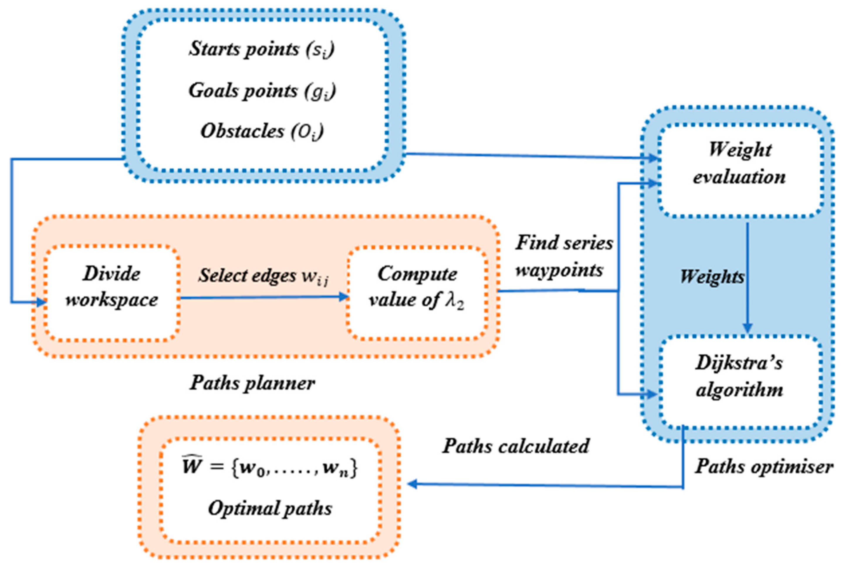
Figure 2.
Scenario of workspace, R1, R2 and R3 are robots, g1, g2 and g3 are corresponding goals and the polygons are the obstacles.
Figure 2.
Scenario of workspace, R1, R2 and R3 are robots, g1, g2 and g3 are corresponding goals and the polygons are the obstacles.
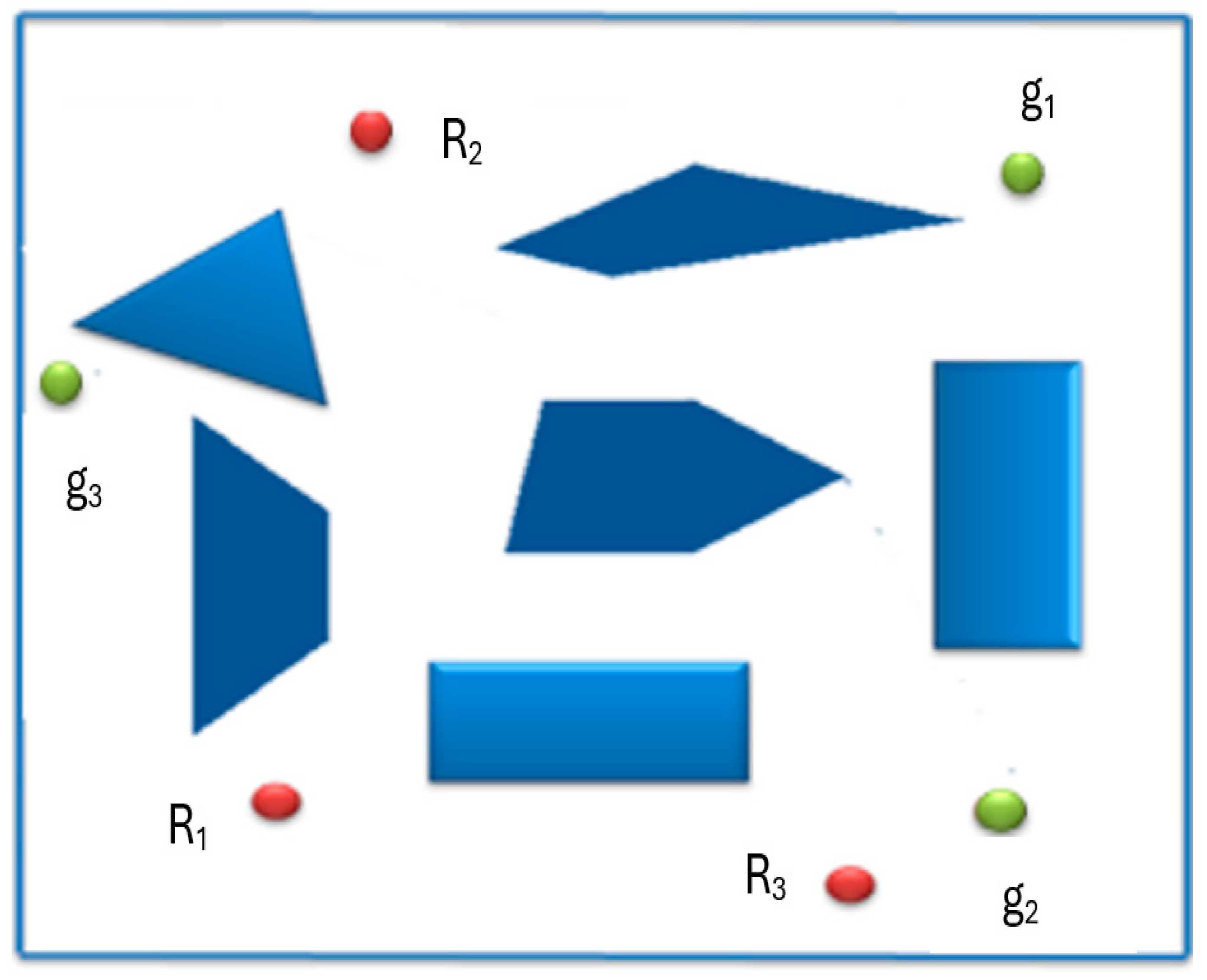
Figure 3.
Workspace represented as a graph. The weights assigned to each edge indicate the cost or distance associated with traversing that path.
Figure 3.
Workspace represented as a graph. The weights assigned to each edge indicate the cost or distance associated with traversing that path.
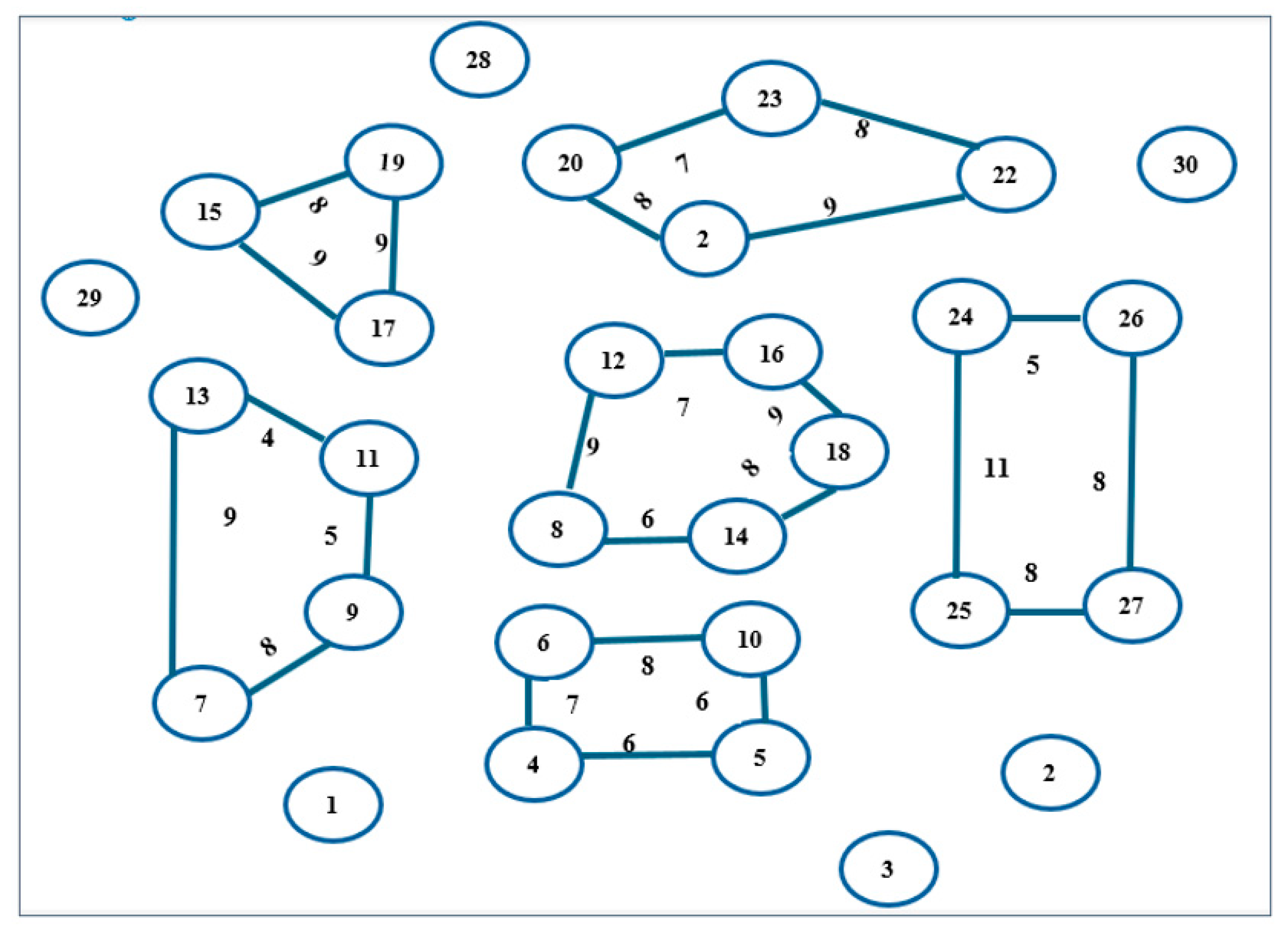
Figure 4.
Example of two disconnected components undirected weighted graph.
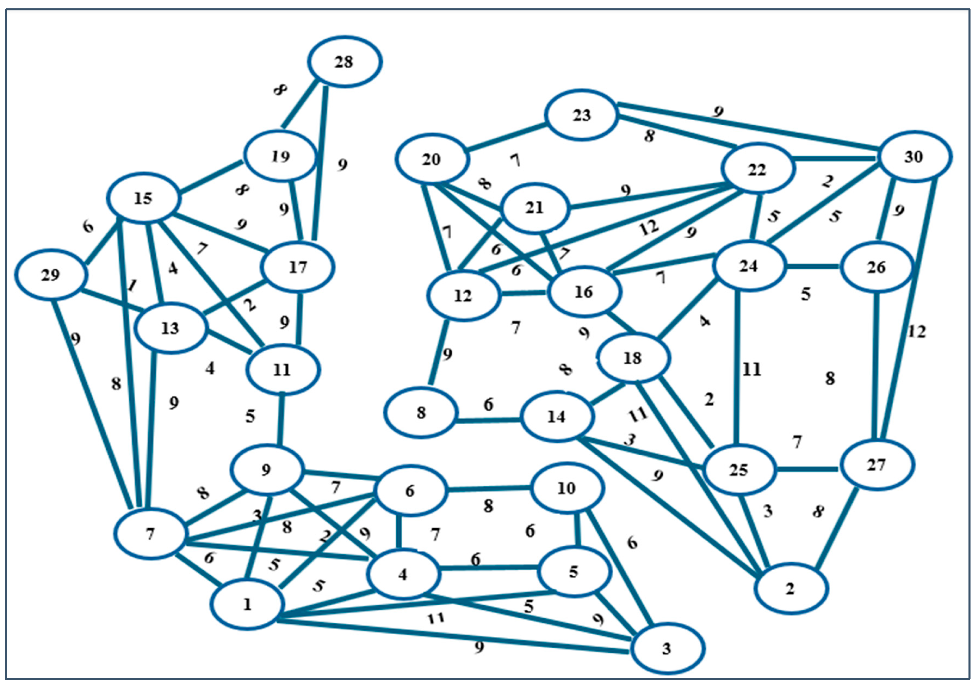
Figure 5.
The shortest paths for three robots using Dijkstra’s algorithm. The numbers next to the links are the weights. The blue circles are the vertices of the obstacles.
Figure 5.
The shortest paths for three robots using Dijkstra’s algorithm. The numbers next to the links are the weights. The blue circles are the vertices of the obstacles.
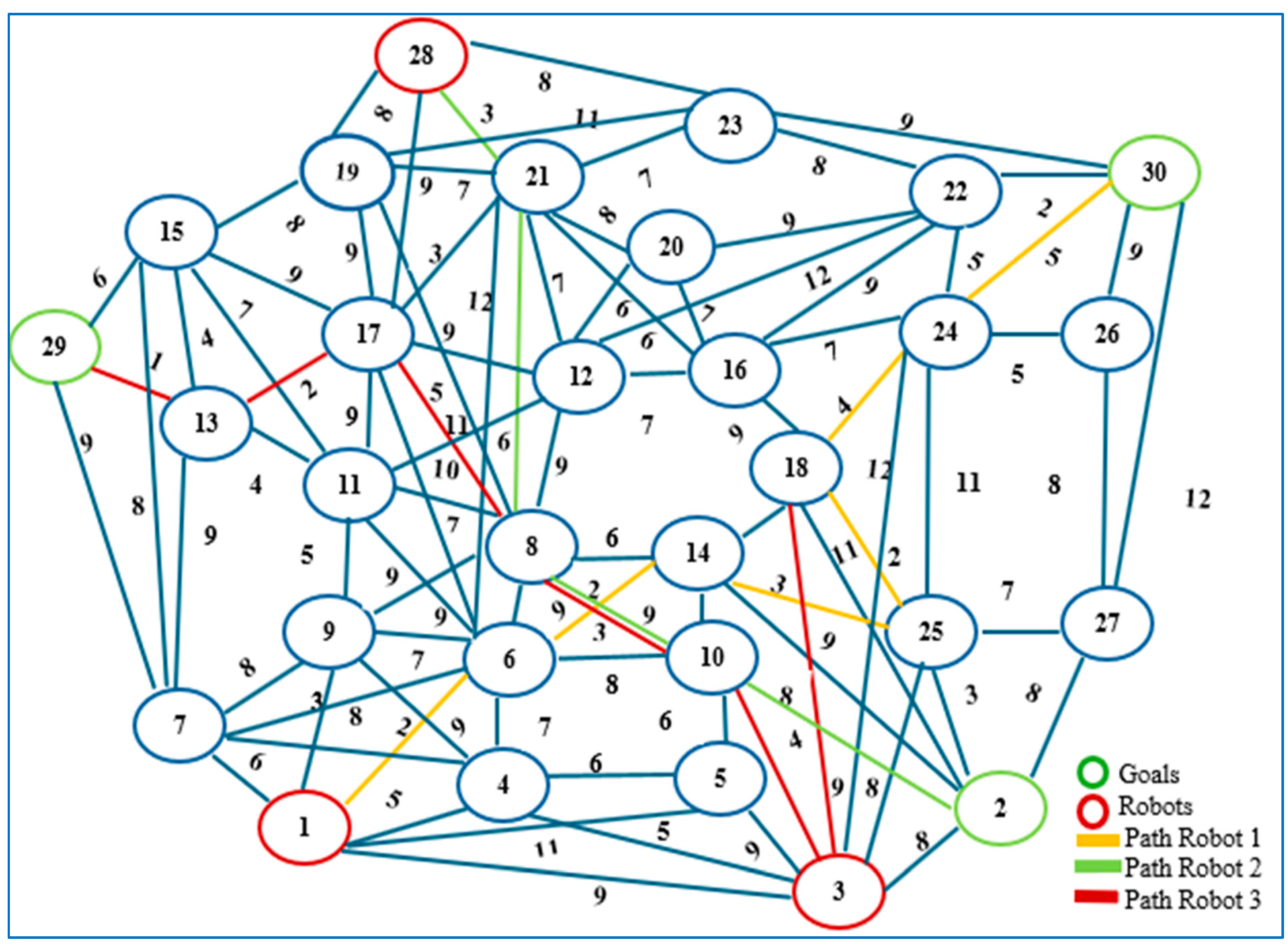
Figure 6.
The shortest paths of the three robots shown in Figure 5 determined using the Dijkstra’s algorithm.
Figure 6.
The shortest paths of the three robots shown in Figure 5 determined using the Dijkstra’s algorithm.
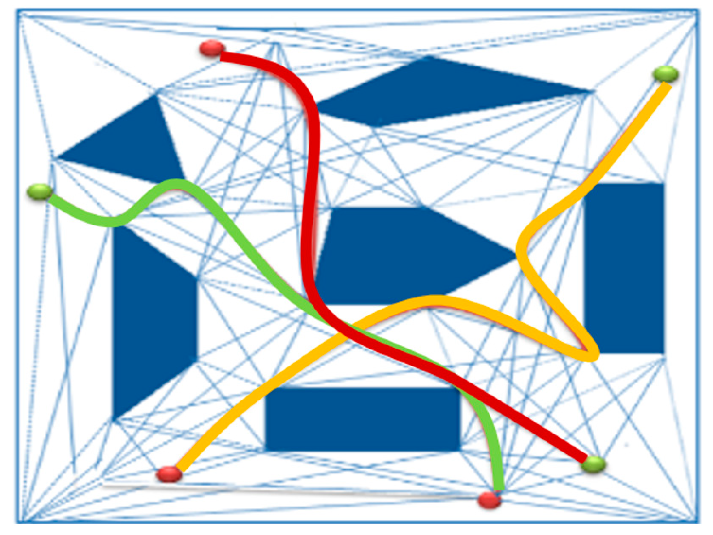
Figure 7.
A workspace environment containing three robots shown as red circles and three goals shown as green circles.
Figure 7.
A workspace environment containing three robots shown as red circles and three goals shown as green circles.
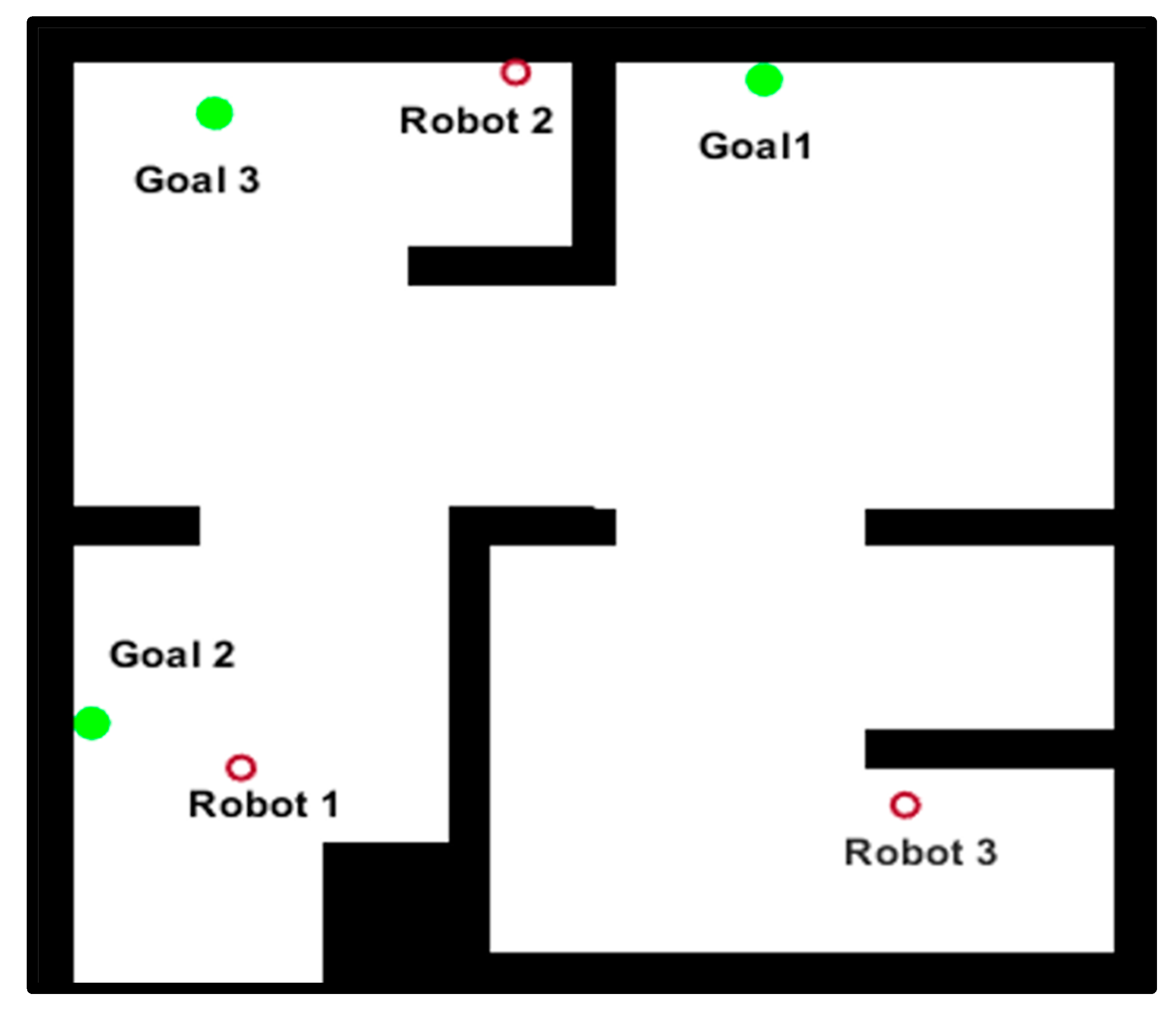
Figure 8.
Two disconnected components undirected weighted graphs consisting of three robots marked as red vertices and three goals marked as green vertices.
Figure 8.
Two disconnected components undirected weighted graphs consisting of three robots marked as red vertices and three goals marked as green vertices.
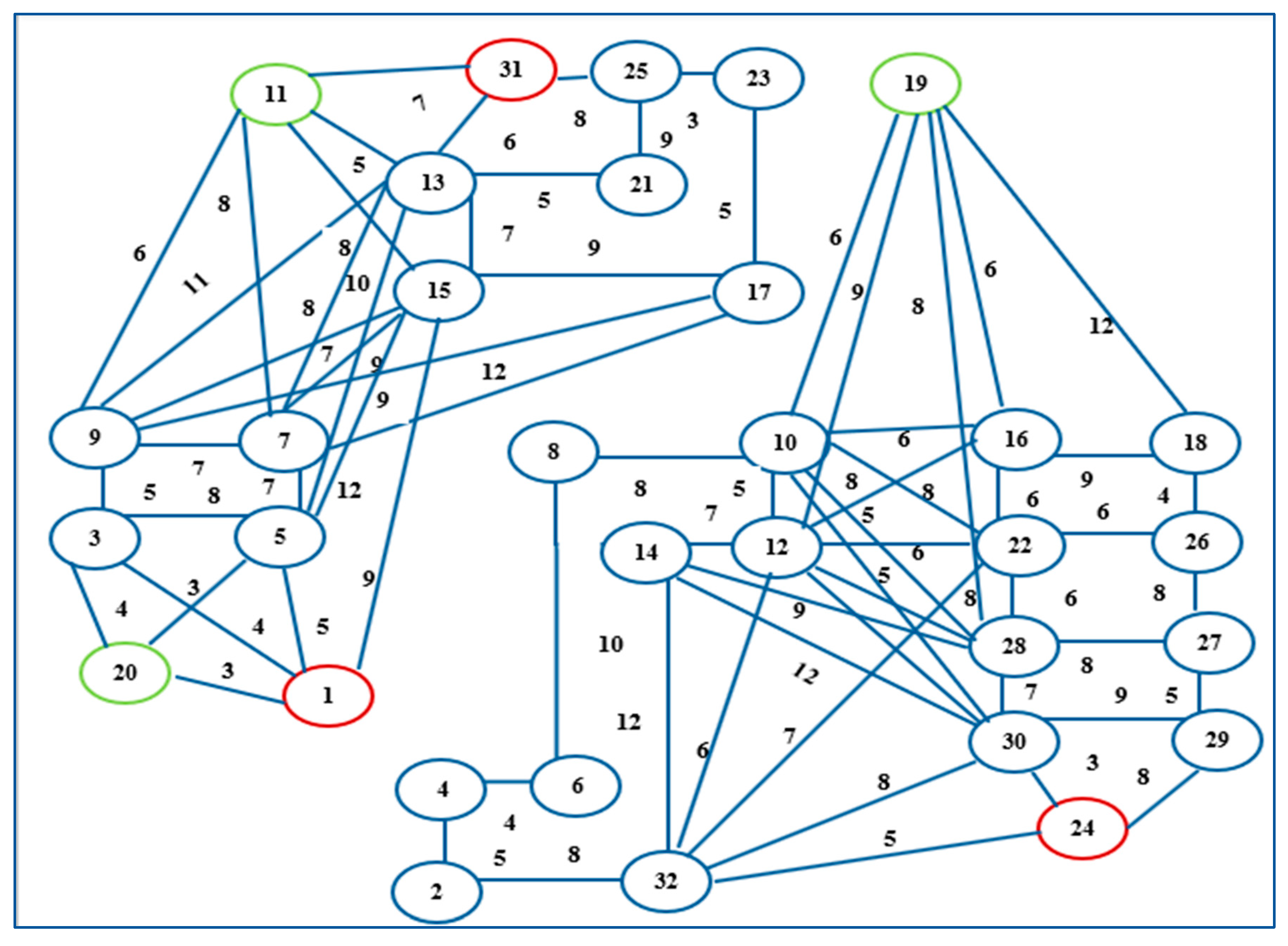
Figure 9.
The shortest paths for robot 1 highlighted in yellow, robot 2 highlighted in green, and robot 3 highlighted in red by using Dijkstra’s algorithm.
Figure 9.
The shortest paths for robot 1 highlighted in yellow, robot 2 highlighted in green, and robot 3 highlighted in red by using Dijkstra’s algorithm.
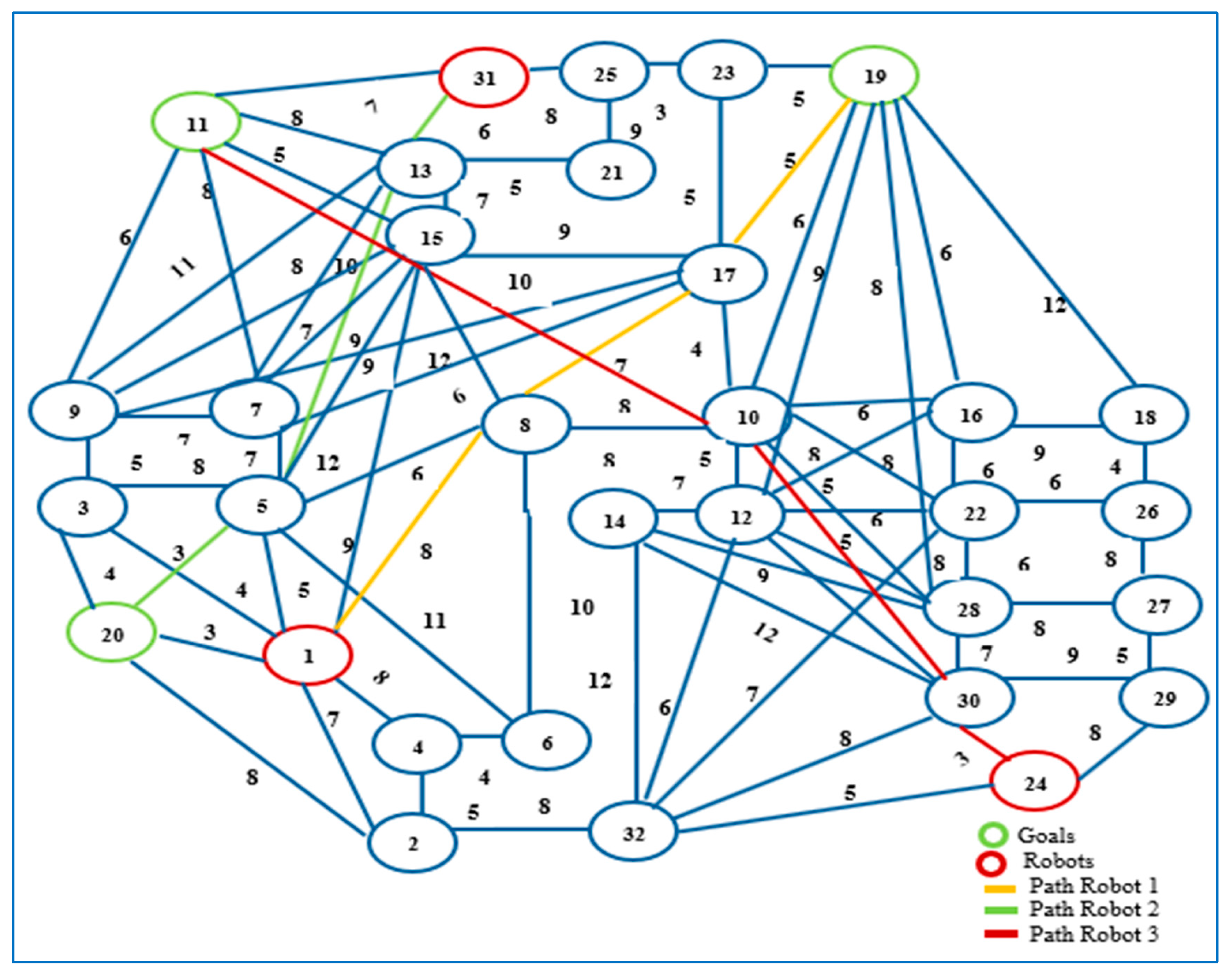
Figure 10.
The shortest paths for three robots by using Dijkstra’s algorithm.
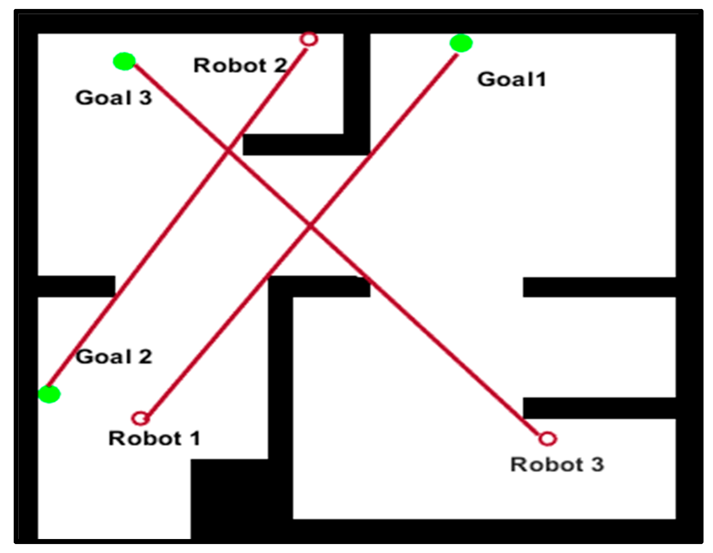
Figure 11.
The workspace, R1, R2 and R3 are robots, g1, g2 and g3 are goals.
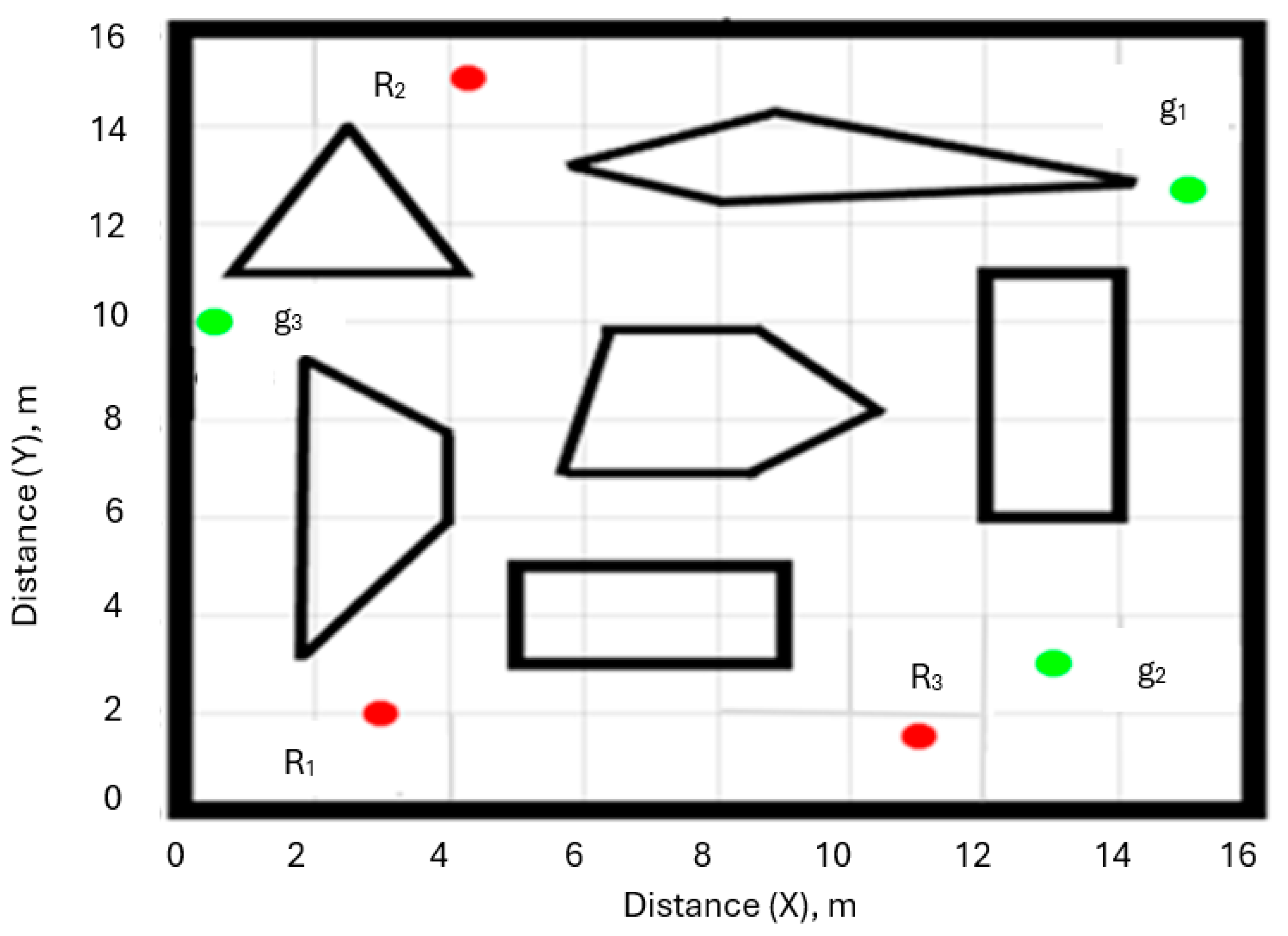
Figure 12.
Workspace represented as a graph contains three robots represented as red vertices and three goals as green vertices.
Figure 12.
Workspace represented as a graph contains three robots represented as red vertices and three goals as green vertices.
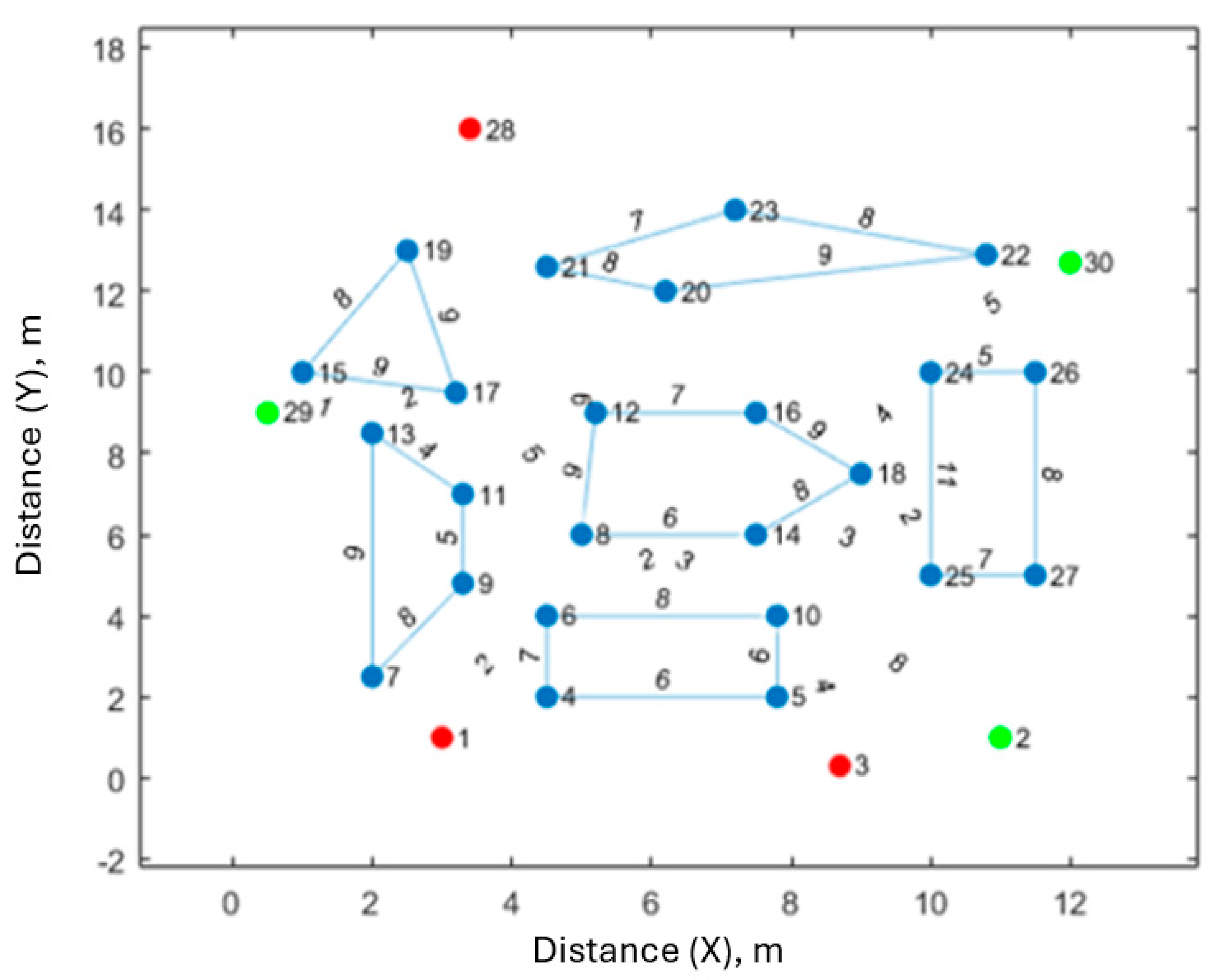
Figure 13.
Paths planned by MRPPA (red for robot 1, green for robot 2, and yellow for robot 3). Path for robot 1 = 1, 6, 14, 25, 18, 24,30 (distance = 18 m), Path 2 = 3, 10, 8, 17, 13, 29 (distance = 15 m), Path 3 = 28, 21, 8, 10, 2 (distance = 20 m).
Figure 13.
Paths planned by MRPPA (red for robot 1, green for robot 2, and yellow for robot 3). Path for robot 1 = 1, 6, 14, 25, 18, 24,30 (distance = 18 m), Path 2 = 3, 10, 8, 17, 13, 29 (distance = 15 m), Path 3 = 28, 21, 8, 10, 2 (distance = 20 m).
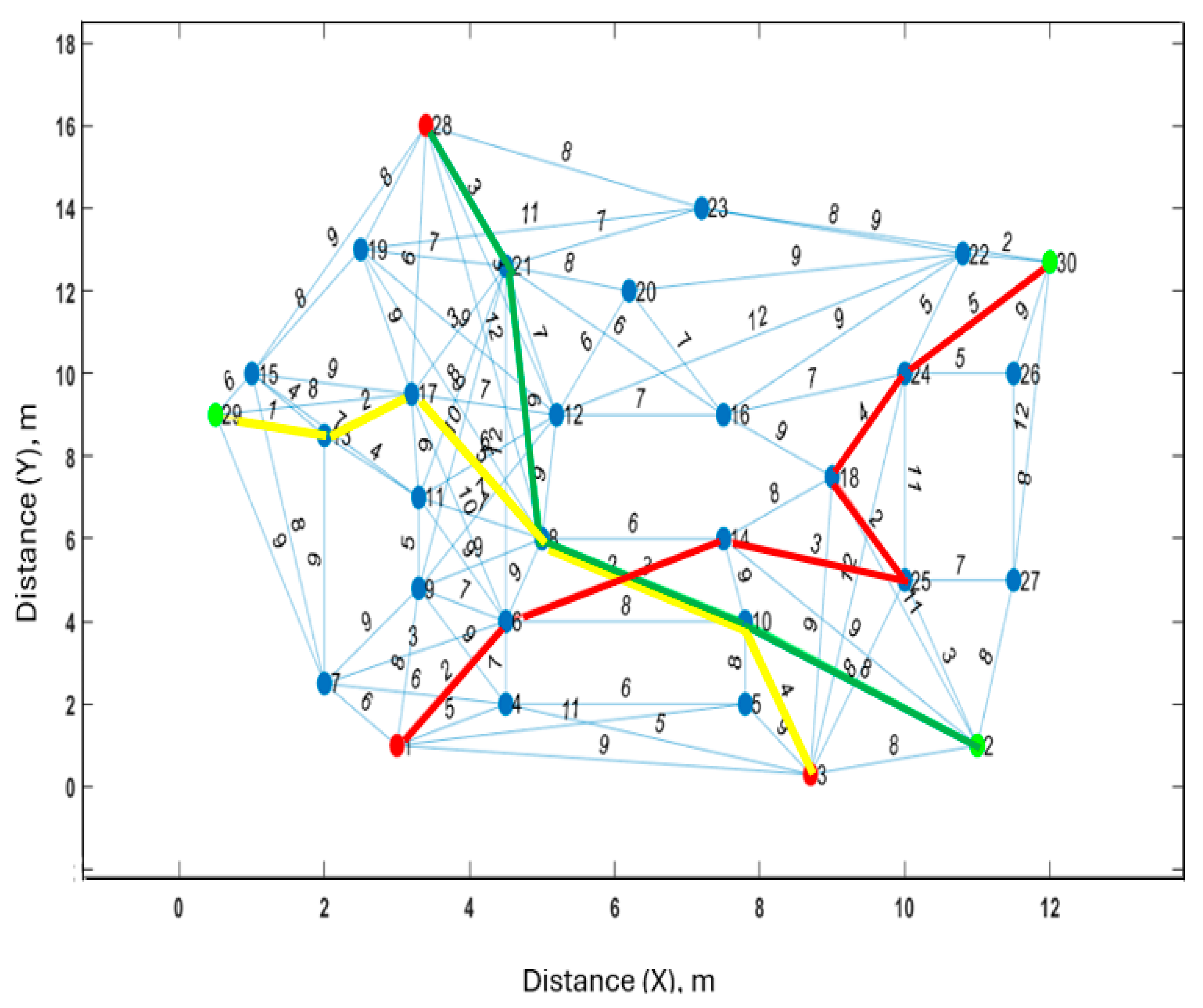
Figure 14.
Simulation for scenario 1 illustrating robots reaching the goals points.
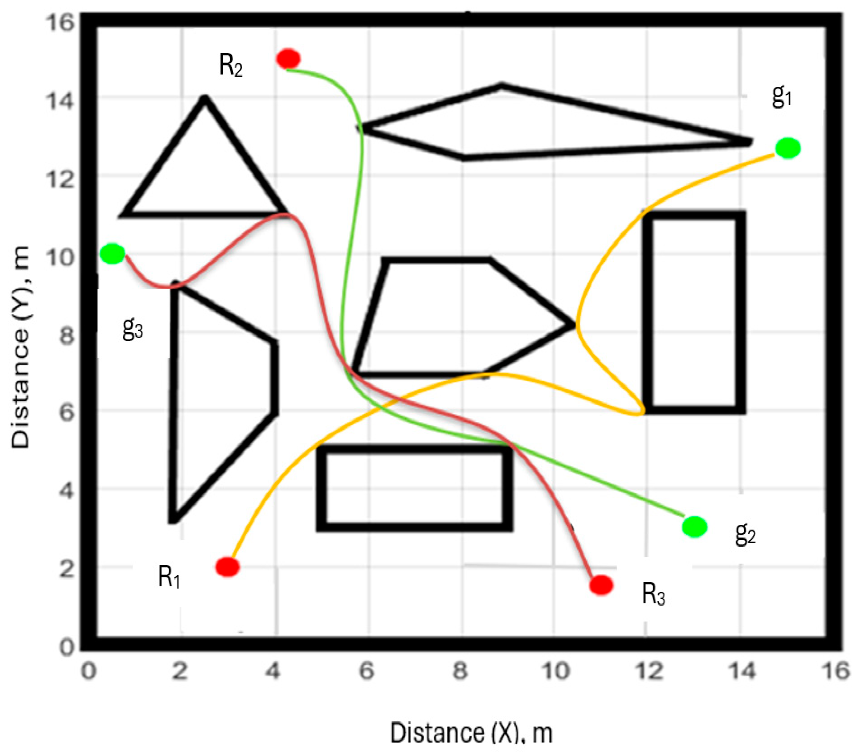
Figure 15.
Scenario 2 workspace environment consisting of three robots highlighted in blue, and three goals highlighted as green, which represented as graph in Figure 16.
Figure 15.
Scenario 2 workspace environment consisting of three robots highlighted in blue, and three goals highlighted as green, which represented as graph in Figure 16.
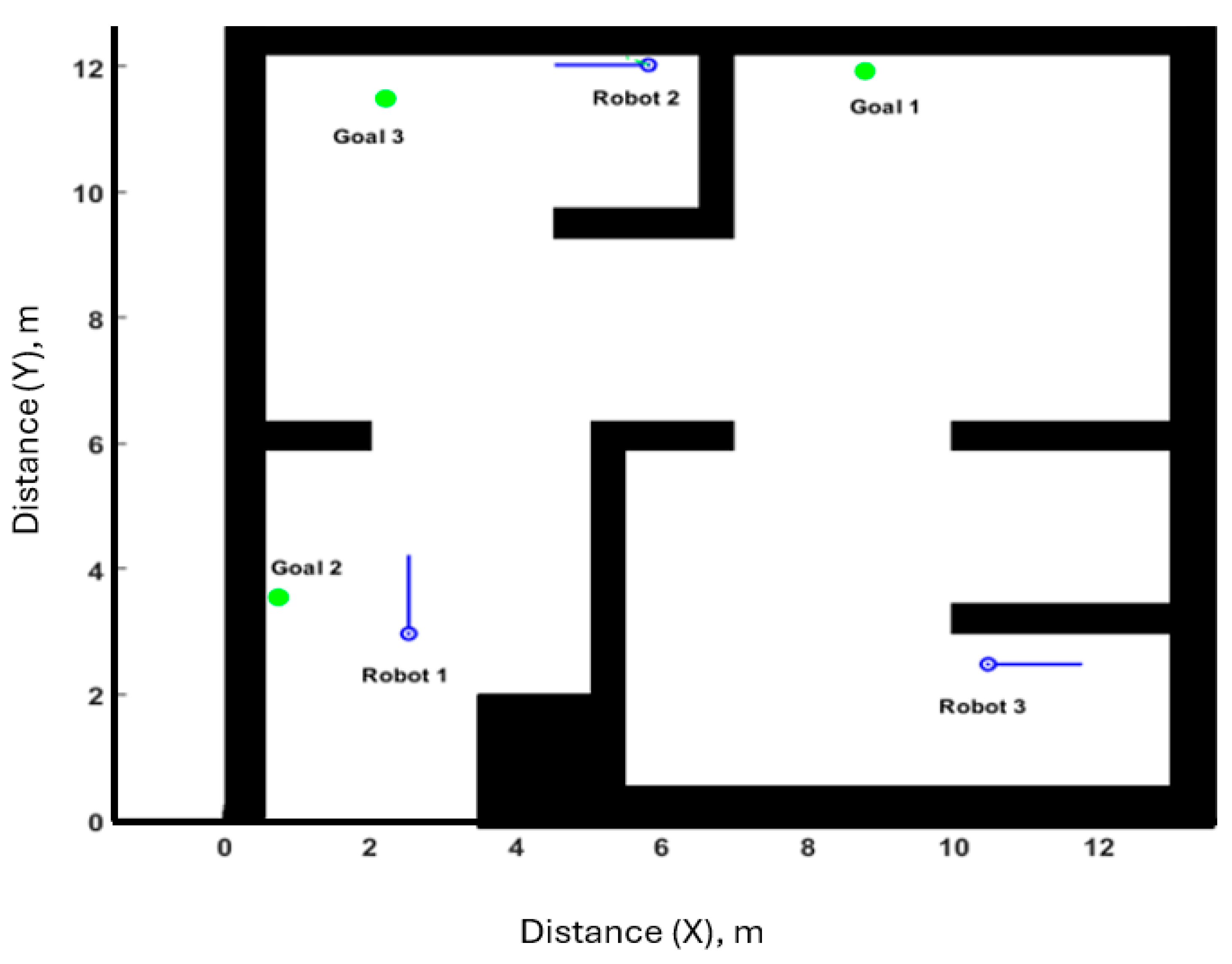
Figure 16.
A workspace represented as a graph consisting of three robots represented as red vertices and three goals as green vertices.
Figure 16.
A workspace represented as a graph consisting of three robots represented as red vertices and three goals as green vertices.
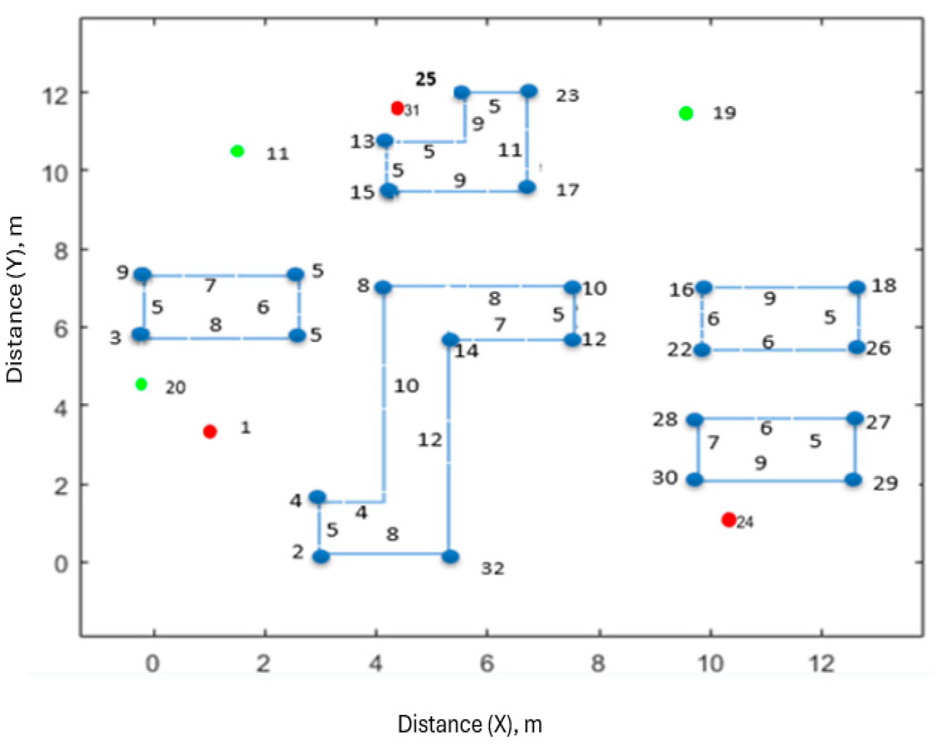
Figure 17.
Senario 2, paths planned by MRPPA highlighted as red, yellow, and green for each robot. Where Path for robot 1 = 1, 8, 17, 19 highlighted as red (distance = 20 m). Path for robot 2 = 31, 13, 5, 20 highlighted as yellow (distance = 19 m). Path for robot 3 = 24, 30, 10, 11 highlighted as green (distance = 18 m).
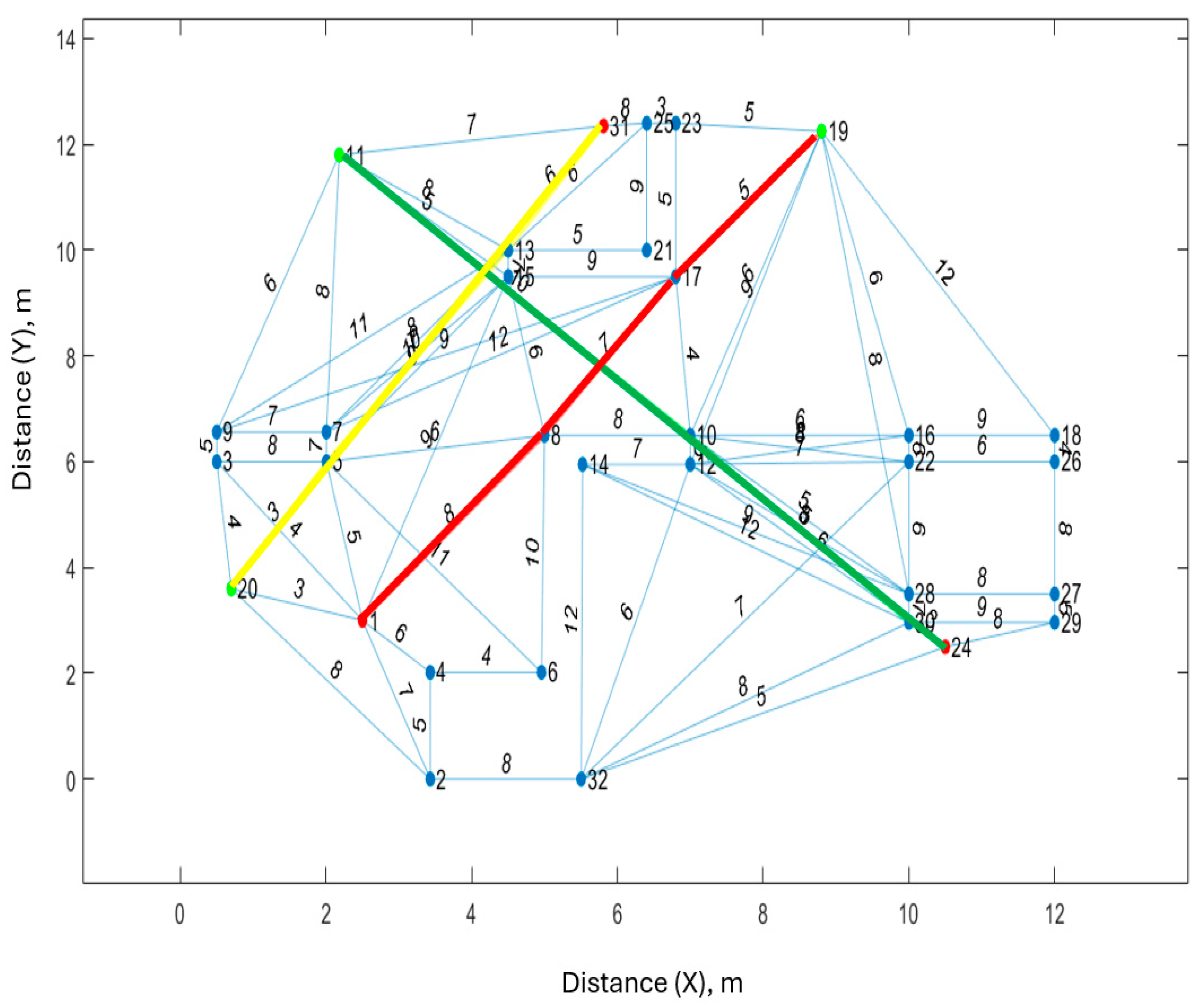
Figure 18.
Simulation results for scenario 2. The green dots are the goals for robots, and the red crosses are the waypoints.
Figure 18.
Simulation results for scenario 2. The green dots are the goals for robots, and the red crosses are the waypoints.
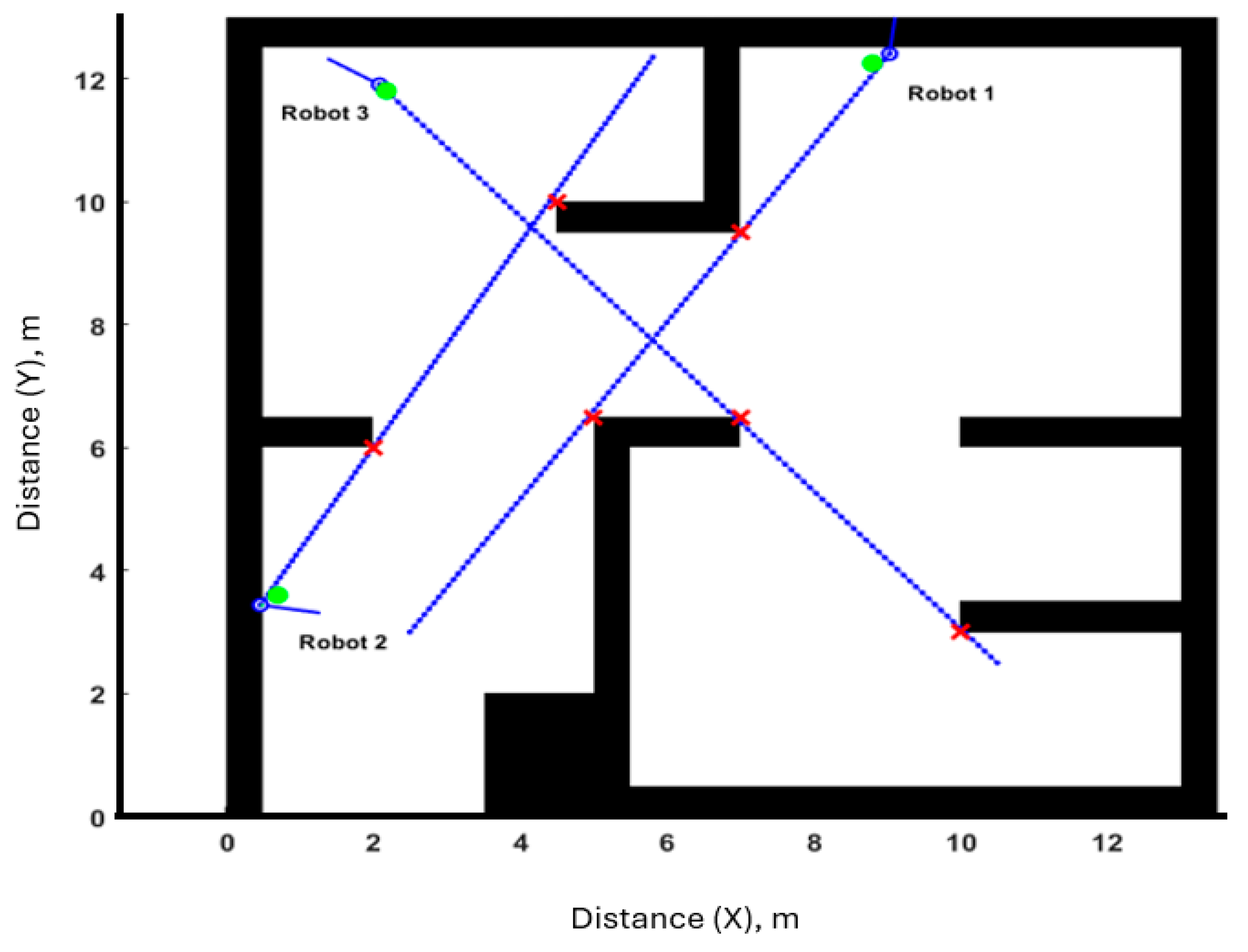

Table 1.
The calculated paths planned (path 1, path 2, path 3) for each robot in Figure 5.
Table 1.
The calculated paths planned (path 1, path 2, path 3) for each robot in Figure 5.
| Initial and endpoint | Shortest Path | Total distance |
|---|---|---|
| 1 | =2+2+3+2+4+5=18 m | |
| 2 | =3+6+3+8=20 m | |
| 3 | =4+3+5=2+1=15 m |
Table 2.
The calculated paths planned (path1, path2, path3) for each robot in Figure 5.
Table 2.
The calculated paths planned (path1, path2, path3) for each robot in Figure 5.
| Robot and its goal | Shortest Path | Total distance |
|---|---|---|
| Robot 1 to goal 1 | =8+7+5=20 m | |
| Robot 2 to goal 2 | =6+9+3=18 m | |
| Robot 3 to goal 3 | =3+6+10=19 m |
Disclaimer/Publisher’s Note: The statements, opinions and data contained in all publications are solely those of the individual author(s) and contributor(s) and not of MDPI and/or the editor(s). MDPI and/or the editor(s) disclaim responsibility for any injury to people or property resulting from any ideas, methods, instructions or products referred to in the content. |
© 2025 by the authors. Licensee MDPI, Basel, Switzerland. This article is an open access article distributed under the terms and conditions of the Creative Commons Attribution (CC BY) license (http://creativecommons.org/licenses/by/4.0/).
Copyright: This open access article is published under a Creative Commons CC BY 4.0 license, which permit the free download, distribution, and reuse, provided that the author and preprint are cited in any reuse.


