
Submitted:
27 May 2025
Posted:
29 May 2025
You are already at the latest version
Abstract
Driven by the latest advancements in wireless technology location-based services have attracted the interest of computing and telecommunication industries, as well as academia, to launch fast and accurate localization systems. The aim of this work is to propose a closed-loop localization framework for large-scale deployments facilitating both the modeling and continuous monitoring of Activities of Daily Living (ADLs). The design of these localization systems is very challenging, time consuming and their adaptation in environmental changes is hard. The proposed methodology takes advantage of limited RSSI measurements at different distances, enriches the data and accurately models the attenuation of the propagated signal. These measurements are then used as input in the data-enrichment process, where the proposed framework generates datasets at different distances. Therefore, all created datasets (gathered and generated) are exploited to train the proposed ML-based chain. The primary purpose of the ML-chain is to determine the distance between the mobile nodes and each installed beacon. The position is then calculated using trilateration methods. Finally, the collected RSSI along with the estimated position will be stored and used for increasing position accuracy, allowing our proposed framework to continuously and automatically optimize its processes and accuracy. Furthermore, to be useful and practical, once reliable position estimation is achieved, the proposed framework can detect predefined Activities of Daily Living (ADLs) based on location patterns and movement behaviors. This capability opens new opportunities for context-aware services and smart environment applications. Each module of the framework was individually tested and evaluated, demonstrating strong performance both in isolation and as part of the integrated system.
Keywords:
Bluetooth Low Energy (BLE)
; RSSI
; Indoor Localization
; Indoor Positioning System (IPS)
; signal filtering
; machine learning
; location-based Services
; ADLs
1. Introduction
Indoor positioning and Activities of Daily Living (ADLs) identification are essential components in Ambient Assisted Living (AAL) environments, designed to enhance the safety, independence, and well-being of elderly or individuals with disabilities [1]. Indoor location-based services (LBSs) allow for real-time tracking of residents within their living spaces, enable emergency response in case of falls or health incidents, monitor mobility patterns to detect potential health concerns, and facilitate context-aware automations, such as adjusting lighting or environmental controls. LBSs can express the importance of location awareness, making things more intelligent and offering more efficient context-aware services, that can provide a plethora of solutions in multiple domains such as public safety and healthcare [2].
There are several widely used techniques that are used in localization systems. The variety of these techniques leverage modalities such as, Received Signal Strength Indicator (RSSI) signal measurements, and Time of Flight (TOF) measurements. Each technique has its advantages/disadvantages and limitations [3]. TOF techniques offer better localization results but require specialized hardware that increases the deployment cost. On the contrary, RSSI-based techniques’ main advantage is the low-cost deployment (no specialized hardware) making a suitable choice for large scale deployments. RSSI-based techniques can be divided into two categories, distance-based, and fingerprinting-based (FP-based) [1]. Fingerprinting-based techniques exploit a vector of RSSI measurements in known fingerprint positions to create a so-called reference fingerprint map (RFM). Then, a machine-learning regressor is fed with the RFM data to build an association rule between RSSI measurements and their corresponding position estimates. Although FP-based techniques can predict effectively the position of mobile nodes, they are inefficient when deployed in large-scale areas.
In contrast, distance-based techniques directly translate RSSI values into position coordinates for mobile nodes using mathematical models that estimate the distance between transmitter and receiver based on signal attenuation [4]. Although distance-based methods are generally less resource-intensive and easier to apply to larger scale areas compared to the technique mentioned above, they tend to suffer from reduced accuracy due to the inherent variability and from the unpredictable evolution of RSSI values caused by multipath effects, interference from various obstacles and environmental changes. As a result, the estimated distances may lead to significant errors in position estimation, especially in indoor environments.
Meanwhile, ADL identification involves monitoring tasks like eating, dressing, and bathing to assess the individual’s health status and detect early signs of cognitive or physical decline [5]. This information supports tailored interventions, such as reminders for essential activities, personalized health plans, and actionable insights for caregivers. Together, these technologies enable proactive care, improved safety, and greater autonomy, fostering smarter and more responsive living environments that support aging-in-place and reduce healthcare costs. Machine learning plays a key role in this process by analyzing complex behavioral data patterns, enhancing activity recognition accuracy, and enabling adaptive systems that respond intelligently to individual needs.
By tracking a person’s real-time location within their living environment using communication technologies like Wi-Fi, BLE beacons, or sensors, and combining it with sensor data (motion detectors, wearable devices, or smart home appliances), it effectively enables the accurate detection can categorization of the type and quality of activities being performed [6]. For instance, detecting prolonged presence in the kitchen along with interactions with smart appliances may indicate meal preparation, while extended time in the bathroom combined with water usage can suggest bathing. Similarly, lack of movement or abnormal positioning (e.g., remaining in bed for an unusually long period) may signal potential health concerns such as falls or mobility issues.
The fusion of location-based data and activity recognition provides a richer context for accurately modeling and identifying ADLs, enabling smart systems to deliver personalized assistance, trigger reminders, or alert caregivers to unusual behavior patterns, ultimately enhancing safety and proactive care management [7]. ADL modeling plays a critical role in translating raw sensor and location data into meaningful insights about an individual’s functional abilities and daily routines. By formalizing how activities are identified, categorized, and interpreted, ADL modeling ensures consistency, enhances accuracy, and enables intelligent systems to make reliable, context-aware decisions that support health monitoring and intervention.
This paper introduces a comprehensive framework that leverages IoT signal processing and ML algorithms to achieve precise indoor localization and effective environmental monitoring. Furthermore, it exploits the person’s position and determines whether he performs one of the ADLs defined. The proposed framework incorporates a feedback process that dynamically adjusts system parameters based on real-time conditions, ensuring adaptability and resilience. By integrating feedback mechanisms, the framework enhances its ability to cope with environmental variability, signal noise, and unforeseen disruptions.
The remainder of this paper is structured as follows: Section 2 reviews related work in IoT-based indoor localization and monitoring systems. Section 3 outlines the proposed framework, detailing its architecture, key components, and feedback-driven methodology. Section 4 presents the experimental setup, dataset description, and evaluation metrics used to validate the framework. Section 5 presents the machine learning training process. Section 6 discusses the results and implications of the findings. In Section 7, the use of positioning information to detect an Activity of Daily Living (ADL) is examined, and a proof-of-concept experiment is presented. Finally, Section 8 concludes the paper with insights into future research directions.
2. Related Work
Location-based services have gained significant attention due to their promising development potential with the advent of IoT and CPS services. However, accurate and efficient localization of objects remains a challenging task due to the dynamic and complex nature of indoor environments. In recent years, literature has proposed various solutions for localization and tracking, introducing different approaches and algorithms [8,9]. In [10] an Obstruction-Aware Signal-Loss-Tolerant Indoor Positioning (OASLTIP) system is proposed towards a cost-effective BLE-based indoor positioning algorithm. Their approach integrates running average filtering, multilateration, and particle filtering to enhance performance. The system is evaluated in both simulated and real-world environments, achieving an average positioning error of 2.29 meters. In [11], an Adaptive Range-Based Localization (ARBL) algorithm is introduced, which combines trilateration with an optimized reference node selection approach. The algorithm leverages combinations of three reference nodes, selecting the most optimal set at any given time based on a criterion that considers both ranging error and localization geometry. Simulation and experimental results demonstrate that the proposed algorithm significantly reduces localization error. The work in [12], proposes a collaborative indoor positioning approach that utilizes a multilayer perception (MLP) neural network to estimate relative distances. Subsequently, they apply trilateration methods to determine the final device position. Experimental results show that the proposed collaborative approach surpasses the standalone trilateration method in terms of positioning accuracy. In [13], authors present a Bluetooth Low Energy (BLE)-based indoor positioning system that combines both trilateration and fingerprinting methods, with a primary focus on monitoring the daily living patterns of individuals, particularly those with disabilities. Their experiments, conducted in various home environments, demonstrate that the system can achieve a location accuracy of approximately 90%. In [14], a scalable and cost-effective Indoor Positioning System (IPS) based on Bluetooth Low Energy (BLE), incorporating frequency diversity techniques, Kalman filtering, and weighted trilateration. Their results show an average error of 1.82 meters for moving devices, 90% of the time, and 0.7 meters for static devices. Authors in [15], investigate user movement in indoor environments by developing a positioning model based on Convolutional Neural Networks (CNN). For their evaluations, they employ machine learning and deep learning techniques to predict their proposed system results and show that their systems can achieve a high accuracy of approximately 97%, with an error rate of about 3%. Authors in [16], present a method for compensating RSSI values by applying Artificial Neural Network (ANN) algorithms to RSSI measurements from three different BLE advertising channels, along with a wearable camera as an additional source to detect the presence or absence of human obstacles. The improved RSSI values are then converted into ranges using path loss models, and trilateration is applied to estimate the device’s location. Their results demonstrate that this approach significantly outperforms other methods, such as fingerprinting or trilateration using uncorrected RSSI values.
Significant efforts have been made in identifying Activities of Daily Living (ADLs). Earlier studies have mainly focused on wearable devices, particularly those equipped with accelerometers and gyroscopes and capture movement patterns. A survey [17] examines the application of machine learning models—including decision trees, support vector machines, and neural networks—for effective ADL classification. Several studies also point to the critical role of signal processing and the extraction of meaningful features in enhancing recognition performance [18]. Foundational works have compared classifiers such as decision tables, SVMs, and k-nearest neighbors when applied to activities like walking, running, and lying down [19]. Additional research has investigated how accelerometers and gyroscopes within wearable devices recognize movement, classifying a broader set of activities. Finally, another work evaluates wrist-worn systems equipped with motion sensors and highlights how sensor fusion can contribute to more accurate recognition, particularly in fall detection [20].
By integrating data from both wearable and environmental sources, sensor fusion techniques have improved accuracy of activity recognition systems. A widely cited study by Roggen et al. [21] illustrated how combining inputs from wearable accelerometers with ambient environmental sensors enhanced the classification of more complex behaviors such as cooking or cleaning. This method leveraged machine learning and sensor data to outperform methods with individual data sources. Based on this approach, Gjoreski et al. [22] investigated similar fusion strategies that combine smart home technologies with wearable devices for fall detection and daily routines monitoring. Their findings showed that applying both feature-level and decision-level fusion methods minimized false alarms and improved the system’s overall reliability.
In research work by Rashidi and Cook [23], ambient sensors like motion detectors were combined with wearable accelerometers and monitored activity in smart home environments. The system used Bayesian networks to integrate data from different sensors, and it performed especially well in recognizing activities that depend on context—like when someone enters or leaves a room.In the same context, more recent studies such as Zhao et al. [24] have used deep learning techniques. By using data from wearable devices and smart home sensors, they showed that deep neural networks can effectively capture complex time-based activities. Overall, combining data from different sensors—known as sensor fusion—has significantly improved the recognition of Activities of Daily Living (ADLs). Moreover, context-aware approaches that take into account both time and space have improved ADL recognition. Rashidi and Cook [23] found that incorporating time-based dependencies using Bayesian networks improved the system’s ability to predict sequences of activities. Similarly, Krishnan and Cook [25] used time-series models with sliding windows to detect overlapping tasks. Researchers have also explored deep learning methods like Convolutional Neural Networks (CNNs) and Recurrent Neural Networks (RNNs) to automatically detect spatial and temporal patterns from raw sensor data. Zhao et al [25], for instance, developed a hybrid system using CNNs and Long Short-Term Memory (LSTM) networks to recognize complex ADLs with high accuracy. These efforts demonstrate the importance of modeling both time and space in activity recognition systems, especially for creating intelligent and responsive smart home environments.Context-aware systems that include indoor location data have proven especially useful for accurate ADL detection. However, challenges remain—particularly in making these systems generalize across different users and homes, protecting privacy, and dealing with unbalanced datasets. To address these issues, researchers are increasingly looking at techniques like federated learning and transfer learning, which aim to create more flexible, secure, and personalized ADL recognition systems without compromising user data.
3. Reference Architecture
Nowadays, the cloud-edge continuum has become the standard approach for intelligent systems that aim to deliver scalable, flexible, and efficient solutions to end-users. These systems must implement various services and applications across different layers, working in collaboration to offer seamless end-to-end solutions. In this context, a multi-layer indoor localization framework was designed and implemented, able to provide Activities of Daily Living on top of the localization services. The architecture of the proposed localization framework, shown in Figure 1 below.
Our framework is divided into three collaborative layers, namely Edge, Cloud and Public layer. Starting from the Edge layer, which comprises from the devices that the system is monitoring to estimate their position, the interfaces (gateways) that are responsible for forwarding the collected data to the upper layers and finally the fixed-position devices (beacons) that are installed in different places around the indoor environment.
The communication at the edge layer is based-on BLE (Bluetooth Low Energy) protocol, where the fixed devices are broadcasting message on a millisecond basis. On the other hand, the non-fixed devices are receiving these messages, extract any localization-based valuable information (e.g. RSSI) and forwarding the data collected to the upper layer, the Cloud layer, through the gateways for further processing.
The Cloud layer is responsible for aggregating data, processing, storing and finally extracting relevant information to the end-users, which, in the specific case, is the estimated positions of the devices. The main aggregation point for the edge data is the Data Aggregation services, where the received data are filtered, enriched with information gathered by Auxiliary Services and finally are stored to the Storage infrastructure. Auxiliary services provide software components for managing device and user profiles, which are closely aligned with the goals of the proposed localization framework. Device management services expose APIs utilized by the localization process, including device information and their relationships with the end-users (e.g. device attached to the hand of a user), and applicable indoor environments. Meanwhile, user management services are storing information related to user profiles, such as health habits and historical records, which are related with ADL monitoring applications.
The aggregated data is forwarded to the localization services, which analyze the collected information and estimate the positions of devices within indoor environments. The proposed localization flow, shown in Figure 2, is divided into three different processes namely, Edge Runtime Environment (EDE), RSSI Measurements Processing and Location Estimation.
EDE is the primary process of the proposed flow, involving the collection of RSSI measurements and the enrichment of the collected data (more details in Section 4.3). The next step, Measurements Processing, focuses on RSSI processing and the extraction of valuable insights that will guide the final stage of the flow—the Location Estimation process. The RSSI processing task ensures signal smoothness by filtering out noisy measurements using a custom filtering mechanism (details in Section 4.2). The processed RSSI data serves as input for the next two parallel processes: the LoS/NLoS classification and Distance Estimation processes (details in Section 5.1 and Section 5.3, respectively). The LoS/NLoS classification aims to detect the presence of obstacles between the communicating entities (beacons and moving devices), while the Distance Estimation process is trying to estimate the actual distance of the communication parties.
The final part of the localization flow is the Location estimation process, where the spatial coordinates of the devices are estimated. This process is divided into two separate sub-processes. The Beacon Selection Optimization sub-process is responsible for identifying a group of beacons (details in Section 5.3), that will be used by the trilateration procedures during the Position Estimation sub-process (details in Section 5.4).
Once accurate position estimation is established, the framework can identify predefined Activities of Daily Living (ADLs) by analyzing spatial patterns and movement trajectories. This enables context-aware insights and supports intelligent behavior recognition within the living environment.
4. Design Phase
This section provides an overview of the three building blocks of our data handling pipeline within our proposed system: data collection, preprocessing, and enrichment. The intention is to provide the localization and classification models with both context-friendly and clean data.
4.1. Data Collection
To collect the necessary data, a TI CC2650 sensor (Rx Sensitivity BLE 1 Mbps) is used as a transmitter, sending signals via Bluetooth Low Energy (BLE). The receiver is an ESP32 Thing device (Tx Power: 0 dBm, Rx Sensitivity (BLE): ~ -97 dBm), which was responsible for receiving the signals and sending the RSSI (Received Signal Strength Indicator) measurements to our cloud infrastructure. To evaluate how the signal behaves under different conditions, measurements were taken across various environmental scenarios and distances:
- Open space: Measurements were performed in an environment without significant obstacles, to record the performance of the BLE signal under ideal conditions.
- Indoor space with obstacles: Static and dynamic obstacles were placed between the transmitter and the receiver to measure the signal attenuation. The scenarios included: a static obstacle (chair and person) at half the distance between the transmitter and the receiver, a dynamic obstacle (one/two person/s) moving freely within the space and finally one/two person/s moving between the transmitter and the receiver.
- Variable distance: All measurements were performed at distances from 0.5 meters to the maximum of 4 meters in increments of 0.5 meters.
4.2. Data Preprocessing
One of the primary techniques used by localization systems to determine object positions in indoor environments involves the analysis of the Received Signal Strength Indicator (RSSI) of incoming communication messages. Respective approaches effectively try to directly relate the distance between the transmitter and receiver to physical modalities’ measurements. A major challenge with received signal intensity is the significant, abrupt and unpredictable fluctuations caused by multipath effects, where signals undergo reflection due to obstacles such as walls, metal surfaces, and moving around human bodies. These fluctuations greatly impact the accuracy of indoor localization systems, necessitating the use of signal processing techniques to mitigate these effects.
The goal of RSSI preprocessing in the context of the proposed framework is to filter out RSSI samples that significantly deviate from the overall sample. This is achieved by promoting a subset of the collected RSSI samples that consist of strong signals with minimal deviations. We prioritize strong signals, relying on signal attenuation models, which essentially show that a signal strength decreases consistently with respect to distance between communication nodes increase. Our assumption relies on the idea that strong signals are the result of direct communication, while the weak signals are results caused by obstacles. Therefore, relying on this principle, if strong signals are present within our RSSI samples, are the ones that will provide a more accurate estimation of the distance. This process is targeting subset (enclosed in red dotted lines) of the signal as shown in Figure 3.
To extract the best subset from the RSSI sample, a weighted rating approach was implemented (the weights are described in Table 1). According to this approach, very weak RSSI samples (outliers -red arrows in Figure 3) are initially removed, and then the RSSI sample is divided into chunks and finally every RSSI chunk is rated. The RSSI sample chunk with the best rating score, is selected and forwarded to the next process of the localization flow, as described in Section 3. The minimum RSSI chunk length that our algorithm uses is 5 sec.
To evaluate the RSSI pre-processing algorithm three different scenarios were performed, at eight different distances. The results are shown in Figure 4. The first scenario performed is the simplest one where the transmitter and the receiver communicate without any obstacle between them. In the other two scenarios communication is performed while an obstacle is placed between them. In the first case, the experiments were performed using a stationary chair and in the second case the same experiment was performed with a human between the transmitter and the receiver.
Each graph in Figure 4 illustrates the Cumulative Distribution Function (CDF) of the RSSI samples. As indicated, our signal pre-processing algorithm selectively removes RSSI samples that deviate significantly from the overall RSSI sample. The objective of these visualizations is to demonstrate how the distribution of raw RSSI samples (left column) becomes more concentrated after the processing task (right column), emphasizing to the retention of ‘clean’ RSSI samples. An expanded CDF curve reflects a more consistent and outlier-free dataset, which is critical for accurately associating RSSI measurements to specific distances.
As illustrated, the distribution of raw RSSI samples (left column) across all scenarios exhibits substantial variability. In the simplest scenario (Empty Space), our pre-processing algorithm results in a marked reduction in RSSI samples density—even at the greatest distances—where the decrease reaches approximately 90%. This reduction becomes even more pronounced at closer ranges, with density shrinking by up to 300% at distances between 0.5 and 2 meters. In scenarios involving obstacles (Steady Human and Steady Chair), the reduction in RSSI samples density is less severe, averaging around 100% across most distances, and exhibiting marginally improved results at shorter ranges. The results clearly indicate a strong correlation between signal behavior and the uniformity of the surrounding environment. These findings facilitate the extraction of meaningful insights regarding both the environmental context (e.g., open space vs. obstructed conditions) and the relative distances.
4.3. Data Enrichment
The data enrichment process is crucial as it provides flexibility and bandwidth requirements reduction in indoor localization systems. It also involves the integration of dynamic data into the overall localization process. Instead of embedding all the necessary information directly into network devices (in edge-layer), the data are retained to the cloud-layer, making it accessible to all system components, through well-defined APIs. The key concept of the proposed localization system is that devices in edge-layer collect only the RSSI samples from installed beacons and forward this information to cloud-layer by utilizing MQTT (Message Queuing Telemetry Transport) protocol. The data is forwarded using the following topic template,
gateways/{gatewayId}/events/devices/deviceId}/position
To identify the indoor environment where the localization process will try to estimate the position of an obstacle or human, we examine the gatewayId of the received message (at cloud layer). As indicated in the reference architecture (Section 3) each indoor environment contains at least one gateway. Using the gateway identifier the data-enrichment process is loading the corresponding indoor environment information which includes the following information,
- General information about the indoor environment, e.g. relevant objects (bed, chairs, etc..).
- The rooms, including their spatial coordinates, are used by the system to identify the room that the obstacles or users are inside.
- Areas of interest with the corresponding annotations (e.g. kitchen) that will be used later by the ADL-related processes, e.g. a polygon that indicates the surrounding area of the kitchen.
- Fixed or moving obstacles that are present in the area. This information will be added to the system either statically or through the localization process.
- Information related to the house tenants, e.g. their current location in the indoor environment.
Next, the process is loading information for the deviceId identifier and devices included in the message payload (localization beacons). For the devices the enrichment process is loading the following information,
- General information about the devices.
- Details related to the device’s hardware components, which are relevant to localization (e.g. transmission frequency, transmission power)
- The spatial coordinates of the beacon, mandatory for position estimation process.
- Details identifying the user or obstacle to which the corresponding device(s) is attached.
The overall data enrichment process is shown in Figure 5.
5. Machine Learning Models Training & Optimization
To design an accurate and powerful indoor localization system based on BLE RSSI data, various interdependent components need to be well designed, validated, and integrated. They range from signal propagation condition classification between Line-of-Sight (LoS) and non-Line-of-Sight (NLoS) to distance estimation from RSSI, beacons selection using intelligent algorithms, to final computation of the device’s position. In this section, we methodically describe and evaluate each core component’s performance.
5.1. LoS-Non LoS Classification
To ensure localization accuracy in complex indoor environments, the proposed system integrates a classification module to distinguish between LoS and NLoS signal conditions. The performance of the machine learning models in LoS and NLoS classification was evaluated using four classifiers with train/test ratio=80/20 and random state = 42: a Random Forest classifier, a kNN classifier, a support vector machine (SVM), and a neural network were trained and compared. Random Forest classifier showed the best overall performance of achieving 83.4% accuracy, 86.7% precision, 84.9% recall, and an F1 score of 85.8% as shown in Table 2.
The results show a well-performing model in terms of high sensitivity and specificity. In support of the superiority of Random Forest, the area under the ROC curve (Figure 6) was also good (AUC = 0.91), which represents its exceptional ability to distinguish between LoS and NLoS conditions. The second-best performing algorithm was the kNN classifier that performed slightly lower but stable performance (accuracy = 81.3%, AUC = 0.88). However, the SVM model was characterized by high recall (92.3%), but with lower accuracy (68.6%), and detected more NLoS cases and possibly more false positives. Meanwhile, the neural network model performed well (accuracy = 72.2%, AUC = 0.81), but showed a good balance of accuracy (73.6%) and recall (82.6%). In general, the results indicate that a set-based model, for example the Random Forest model performed robustly and accurately in the LoS/NLoS classification process in dynamic environments with variation in obstacles.
5.2. Distance Estimation
For the distance estimation problem, a different approach was followed since contrary to be binary problem of LoS-NLoS classification, in this case, we have a regression problem (the values range from 0.5 – 4.0). The procedure is the same, several algorithms were tested and the results produced were used for the comparison of the algorithms shown in Figure 7.
According to the metrics shown in Figure 7, LSTM and Gradient Boosting appear to have the lowest RMSE value (0.6229) and the highest R² (0.7107 and 0.7097 respectively), which means that this algorithm has the best overall performance in distance prediction.
To establish the accuracy of RSSI-based range estimation and LoS/NLoS-aware features, a variety of machine learning models that include both traditional as well as deep learning approaches were tested. Performance was quantified in terms of three significant parameters: Mean Absolute Error (MAE), Root Mean Squared Error (RMSE), and the coefficient of determination (R²). Figure 7 depicts that tree-based models such as Random Forest and Gradient Boosting outperform linear and kernel-based models in the sense of having lower values for MAE and RMSE and higher values for R², which indicates superior generalization and lower prediction bias. The performance of the LSTM model was not far behind the best-performing models in terms of RMSE and achieved a good value for R². The methodology illustrates the effectiveness of temporal modeling in addressing the sequence-dependent variability in RSSI data. However, performance was poor for lighter models like Linear Regression and Decision Trees in terms of RMSE but good in terms of R² values.
5.3. Beacon Selection Optimization
Too many active beacons in a confined space can cause signal interference, leading to noisy RSSI readings and reduced localization accuracy. Selecting a non-overlapping or spatially distributed subset helps improve signal quality. The Beacon Selection Problem (BSP) involves the selection of a subset of beacons based on specific optimization criteria. Although it is commonly believed that the utilization of more beacons in multilateration methods improves the accuracy of the localization process, this is valid only when the estimated distances between the beacons and the trackable objects are accurately estimated. Signals can be affected by multipath propagation, environmental interference, and hardware induced error, hence a distance estimation based on those distorted signals, will propagate an error to the localization result. Therefore, implementing a robust BSP method is essential to filter out unreliable signals, ensuring that only the most accurate and stable beacons contribute to the positioning process.
In this section, a multi-criteria weighted scoring system is introduced to solve the BSP. It evaluates the beacons based on their signal and its produced characteristics such as the Line-of-Sight (LoS) availability, RSSI signal strength, signal variance, packet loss rate and other techniques. In order for a scoring system to be effective, factors used in the tool should be as independent, precise, and objective as possible. For each of the methods used, a maximum score (named Involvement Ratio) has been assigned and the maximum score a beacon can get is 1.
Various tests were conducted to find the optimal involvement ratios for each scoring criterion. The scoring parameters as well as their respective involvement ratios are presented in Table 3.
An example scenario is presented to prove the adequate functionality of the scoring system and the involvement ratios. It consists of 9 beacons, 5 of which were in LoS with the target at distances of 0.5m, 1m, 1.5m, 2m and 2.5m, while for the rest 4 there was a human between the beacon and the target (NLoS) and their respective distances were 1m, 2m, 3m and 4m. Each beacon’s sample consists of 2 seconds worth of received packets (the expected number of packets is 20 but not all are received, especially on indirect and distant beacons, hence the Loss Rate).
In this scenario it is obvious that the three highest scores (Top 35%) were given to the closest beacons that were in direct line of sight. They are followed by three beacons, at 1m, 2m and 2.5m, the first not being in Line of Sight. Even though it was expected that this beacon would be lower, details such as the Loss Rate, variance etc. determined the score, hence the beacon with ID 4 has a more reliable signal. The result is followed by 3 beacons that were not in Line of Sight with the target. The scenario and the results are visualized at Figure 8.
5.4. Location Estimation
In indoor localization systems, the problem of determining the position of an unknown point based on its distances from multiple known reference points can be addressed using two main techniques: Trilateration and Non-Least Squares [26]. Trilateration determines the target’s location by measuring the radii of circles (or spheres in 3D space) centered at known reference points, with their intersections revealing the unknown position. In contrast, non-least-squares approaches do not rely on minimizing squared errors. Instead, they are designed to handle environmental factors such as signal interference, measurement noise, outliers, and non-line-of-sight conditions, which can distort distance calculations. These techniques are particularly useful in challenging environments where traditional trilateration methods may struggle to provide accurate results.
In this paper, a non-least-squares technique is applied to estimate the unknown position of a non-static node. We formulate the localization problem as a nonlinear least squares optimization and solve it using the Levenberg-Marquardt Optimizer, a highly efficient and reliable method for refining position estimates in real-world localization scenarios. The Levenberg-Marquardt Optimizer combines the Gauss-Newton method and gradient descent, dynamically adjusting between them to enhance convergence. When the solution is far from optimal, it operates like gradient descent to maintain stability; as it nears the optimal solution, it transitions to the faster Gauss-Newton method for improved accuracy. This adaptability makes it particularly effective in handling noisy distance measurements.
6. Evaluation/Experimental Results
6.1. Setup
The proposed localization process was evaluated in the Ambient Assisted Living (AAL) environment within the ESDA-LAB premises [26]. The AAL environment is shown in Figure 9. The setup consists of TI Sensor Tag (CC2650) devices acting as beacons, each in a fixed position. These devices broadcast simple messages at a frequency of 10 messages per second.
On the receiver side, the device whose position we aim to estimate is a SparkFun ESP32, typically attached on obstacles or users in standard localization setups. Its role is limited to receiving messages from the beacons, extracting the RSSI from each beacon’s transmission, and forwarding the collected data to the application running the proposed localization algorithm to estimate its position.
6.2. Signal Filtering
Signal filtering is an essential procedure for RSSI-based indoor localization systems to mitigate signal fluctuations caused by multipath interference and environmental noise. Three filtering techniques were tested in this work: the Kalman filter, the Weighted Moving Average (WMA) and the Gaussian Filter. Various tests revealed the optimal parameters for each filter, aiming to minimize the distance estimation error.
Kalman filter is one of the most used filters in relevant applications, as it is particularly effective in dynamic environments where RSSI readings fluctuate rapidly due to movement or interference. By continuously updating its estimates based on prior values and new measurements, the Kalman filter can provide stable and accurate RSSI readings. The optimal parameters of the filter in our case are F = 1, H = 1, Q = 0.1 and R = 8.55 after tests.
The weighted moving average (WMA) filter is one more popular filtering technique with sufficient results. It smooths RSSI values by assigning higher weights to more recent measurements while still considering past values, while a window defines the number of the latest values being used in the calculation. In our dataset, greater window sizes lead to less error and deviation. On a deployed system though, where the targets are moving objects, it is inefficient to use wide windows. In our case, a window size of 20 offers the optimal balance between the accuracy and the time needed to collect those measurements.
The Gaussian filter applies a Gaussian-weighted convolution to the RSSI readings, giving more emphasis to values near the center of the window while gradually reducing the influence of outliers. This method is particularly useful for environments where RSSI fluctuations follow a normal distribution, as it effectively removes high-frequency noise while preserving important signal variations. The algorithm has been tested and used in various relevant works.
A dataset consisting of measurements at 0.5m, 1.5m and 2.5m is used to produce metrics on the filters’ efficiency. The measurements are taken at an empty space thus the received signal, raw and filtered, owes to be the most stable possible. As we can see from Table 4, at 0.5m, all filters perform similarly with low MSE and variance, but as the distance increases, MSE and variance rise significantly. Kalman performs best at 1.5m with MSE at 4.57 ⋅ 10-2 and its variance being slightly higher than Gaussians. More notable differences are observed at 2.5m, in which Gaussian outperforms all 3 filters at 4.90 ⋅ 10-1 MSE and 6.75 ⋅ 10-2 variance. Overall, the Gaussian filter provides the best trade-off between error reduction and consistency (performs better at large distances such as 2.5m), while the Kalman filter performs well at short to medium distances but becomes less reliable at longer ranges.
In Figure 10, the three signals are shown in the same scenario (empty space) but at different distances (0.5, 1.5 and 2.5 meters). We observe that there are some points where a signal has spikes that intervene another signal and negatively affect its structure. For this reason, we applied filters to normalize the sample to make it more distinct. From the filters applied, we ended up with three that had the best results and are depicted in the middle of each signal: Gaussian (orange), Kalman (blue) and Weighted Moving Average (pink). We observe that the WMA filter responds faster and abrupts changes in the signal compared to the Gaussian filter where the change is done more smoothly (this is more obvious in the area between 200-400 in the x-axis of the sample and at a distance of 1.5m). On the other hand, the Gaussian manages to make smoother changes when there are fluctuations in the signal and in this way, we can have a smoother transition (this is observed more at the distance of 2.5m between 150 and 200 of the x-axis).
6.3. ML Algorithms Results (Distance Estimation)
The same approach as LoS/NLoS classification was followed, using a train/test ratio = 80/20 and random_state = 42, with the main difference that now the problem we must deal with is a regression problem. With this approach we tested the following algorithms, and the results are shown in Table 5.
Among the models compared, the Random Forest Regressor and the K-Nearest Neighbors Regressor had the best and most consistent performance for all metrics. Both the Random Forest Regressor and the K-Nearest Neighbors Regressor recorded the lowest MAE (0.50), MSE (0.57), and RMSE (0.76) while having a relatively stable R² score of 0.56. While the Gradient Boosting Regressor performed slightly better in terms of MSE (0.56), it was less stable, particularly regarding MAPE (34.07%) and MedAE. Linear Regression performed the worst on all the performance metrics, reflecting its low capacity to represent the nonlinear relationship prevalent in RSSI-based range estimation. Overall, the results validate the suitability of ensemble and non-parametric models (Random Forest, KNN) for representing the complicated, noisy patterns of indoor signal propagation.
6.4. Position Estimation
The evaluation of the overall localization system is performed in the surrounding area of AAL House as illustrated in Figure 9. Measurements were carried out across four separate paths, which have been individually segmented, as illustrated in Figure 11. The left part of the figure displays the actual trajectory, whereas the right part provides a visual comparison between the predicted trajectories produced by the proposed localization system and the corresponding ground truth data.
The accuracy of the proposed localization system is assessed using the Root Mean Square Error (RMSE) and the mean localization error as quantitative performance metrics. The results of the localization system estimates are illustrated in Figure 12.
The RMSE values ranging from 0.66m up to 0.95m and mean errors between 0.50 m and 0.87 m. From all the evaluated routes, Route #1 exhibits the lowest RMSE and mean localization error, which can be attributed to the high density of beacons employed by the localization system and from the relatively unobstructed space. An additional insight that validates the effectiveness of the beacon selection process (as part of the beacon optimization selection part) is the convergence of localization errors toward the positions of the nearest beacons. Routes #3 and #4 exhibit similar RMSE and mean localization error, primarily influenced by the low density of the selected beacons utilized by the localization system. In contrast, Route #2 exhibits the highest RMSE and mean localization error, which can be attributed to the presence of multiple obstacles within that section of the indoor environment.
7. ADLS
7.1. ADL Design
Modeling an Activity of Daily Living (ADL) using positional data in an indoor environment involves leveraging spatial context alongside sensor information to infer activities based on a person’s location and movement. Indoor positioning data (from Wi-Fi, Bluetooth, RFID, or other positioning systems) provides information on where the individual is located within a specific area, which can be used to classify activities based on typical spatial patterns associated with each activity.
The first step is to define the ADLs that must be modeled (e.g., eating, cooking, sleeping, walking, or sitting). Each ADL is often linked to a specific location within an indoor environment (Table 6).
ADLs are not only location-based but also time-dependent. It is important to recognize that a person might start their activity in one location and move to another (e.g., cooking might start in the kitchen and then transition to sitting at the dining table). To model the temporal context, the time window must be defined as well as the activity transitions. The next step is to extract features collecting data from the indoor positioning system as the person moves around the environment. This data might include location coordinates, indicating the person’s position in the room or house, timestamps, to correlate the position with time (e.g., duration in each location) and movement patterns, e.g. movements between rooms or specific locations within a room. The final step is utilizing the positional and temporal features and training a machine learning model to recognize activities based on the person’s location and movement patterns. In this work 3 ADLS were defined. Table 7 shows the ADLs, the features related to each one and the machine learning result.
7.2. Evaluation
The ADLs evaluation was done classifying user movement paths between rooms using coordinate data provided in CSV files. Each file represented a single path, containing time-stamped coordinates as well as the starting room and ending room. The goal was to build a model that could predict the origin and destination of a path based on its coordinate sequence.
Initially, multiple CSV files were uploaded, each labeled with a specific path such as “office to bed” or “sofa to kitchen.” The coordinate data was parsed from strings like [-6.13, -7.76] and structured into numeric arrays. A preliminary plot was generated where each path was visualized using a line connecting its coordinate points. Figure 13 shows that although the starting and ending areas were relatively distinct, some paths overlapped or intersected, especially around central areas.
Machine learning models were then used to classify the paths. Basic feature extraction involved computing the mean and standard deviation of the x and y coordinates for each path. These were fed into models including a Random Forest, k-Nearest Neighbors (k-NN), and a Multi-Layer Perceptron (MLP). The models performed poorly (all of them had an accuracy of 40% at most). Predictions frequently misidentified paths that overlapped in space, despite having distinct labels.
To improve feature quality, full coordinate sequences were flattened into fixed-size vectors. This allowed models to consider more information about each path. Additional features such as path length, direction vectors, and start/end points were also computed and used to refine the model inputs. However, even with these enhancements, accuracy remained low due to the similar shapes among paths.
As an alternative to machine learning, a simple rule-based method was implemented. This method stored the start and end coordinates of each known path. When a new path was provided, its start and end coordinates were compared to each known pair using Euclidean distance. The label of the closest known path was returned as the predicted path. This approach assumes that the user’s movement between rooms tends to start and end in consistent physical locations, which was mostly true based on the data.
To test the rule-based classifier, six test samples were used (e.g. “office to bed”, “office to kitchen” etc.). This was further supported by a confusion matrix shown in Figure 14. The rule-based method correctly identified most of them correctly, giving an accuracy of 100%. In two circumstances (bed->fridge and bed->kitchen) the model was confused but still made the correct prediction with high accuracy. The confusion derives from the fact that both paths had the same starting point and very close ending points as shown in Figure 15.
In addition to this, a visualization was created showing only the start and end points of each path. Green dots represented start points, and red dots represented end points. These were connected by dashed lines, and each point was labeled with the associated room. The visualization confirmed that while path shapes overlapped, start and end positions were often distinct enough to uniquely identify the path.
Based on these observations, a hybrid approach was used combining a rule-based system with a machine learning model to improve path classification accuracy. If a full path has starting and ending coordinates close to a known path, the system confidently assigns the corresponding label using simple distance checks. If the path is ambiguous, the model predicts the most likely destination based on learned patterns. This method balances precision and flexibility, making it ideal for small or overlapping datasets.
The last challenge was to identify a user’s destination based on their movement path, using coordinate data from CSV files. First, the features from each path were extracted, including coordinates, starting and ending points and direction. Several machine learning models were trained and combined with a rule-based system to create a hybrid classifier. This hybrid approach uses simple distance checks to confidently match known paths, while relying on the trained model for more ambiguous cases. To handle partial paths, the first half of the file’s coordinates were extracted and the model predicted where that half-path leads. Even if multiple paths start from the office and end at bed, their paths may differ slightly — especially in the first half.
In Table 8 two probability tables are shown for the paths Bed to Kitchen and Office to Bed. It is clearly shown that the results are better when the path doesn’t overlap with others.
8. Limitations and Future Work
Despite the promising results and the comprehensive design of the proposed localization and ADL monitoring framework, several limitations need to be addressed. One of the primary challenges lies in the sensitivity of RSSI-based positioning to environmental factors such as multipath effects, interference, and dynamic changes in indoor layouts. Although signal filtering and data enrichment processes help mitigate these issues, they cannot fully eliminate the inherent variability of RSSI signals, which may lead to occasional inaccuracies in localization, particularly in cluttered or highly variable environments.
The system also assumes consistent beacon placement and hardware characteristics. In real-world scenarios, hardware variability or battery degradation could affect signal quality, potentially impacting the performance of the machine learning models that were trained under idealized conditions. Similarly, user-specific behavior variations, such as differences in movement patterns or ADL performance, are not currently personalized, which may limit the framework’s accuracy for broader deployment.
Another limitation is the reliance on preconfigured areas of interest and static annotations for ADL detection. While the proposed method is effective for controlled or semi-structured environments, it may struggle to generalize across diverse residential layouts or to adapt to frequent environmental changes without manual intervention. Additionally, the rule-based classifier that was employed in ADL recognition may not scale well for more complex or overlapping paths where behavioral ambiguity increases.
In terms of future work, one promising direction is the integration of generative adversarial networks (GANs) to synthetically expand RSSI datasets, enhancing the robustness of ML models under varied conditions. Moreover, the feedback loop mechanism, which currently adjusts system parameters post hoc, could be improved with real-time adaptive learning techniques, allowing for dynamic model retraining based on streaming data. Another critical advancement would be the inclusion of context-aware and personalized ADL models that adapt to individual behavior and preferences over time, leveraging sensors measurements.
9. Conclusions
This work presents a scalable framework for indoor localization designed to work seamlessly in real-world environments. By using RSSI signal processing, machine learning and ADL recognition, the system proposed effectively overcomes common challenges such as signal noise and changes in indoor conditions. The integration of machine learning for tasks like distance estimation, LoS/NLoS detection, and activity recognition enables position and ADLs monitoring. The experiments conducted showed that each component of the system performs well both separately and combined with the other components. As for future work, the system is planned to be more personalized, adaptable, enhancing safety, independence and quality of life.
Acknowledgments
This work was co-funded by the European Union’s HORIZON EUROPE research and innovation programme under the grant agrement No 101147881 - InclusiveSpaces: Designs, Tools & Frameworks for Creating an Accessible & Inclusive Built Environment for All, for Now & for the Future.
References
- Zafari, F., Gkelias, A., & Leung, K. K. (2019). A Survey of Indoor Localization Systems and Technologies. IEEE Communications Surveys & Tutorials, 21, 2568-2599. [CrossRef]
- Farahsari, P. S., Farahzadi, A., Rezazadeh, J., & Bagheri, A. (2022). A Survey on Indoor Positioning Systems for IoT-Based Applications. IEEE Internet of Things Journal, 9, 7680-7699. [CrossRef]
- Asaad, S.M.; Maghdid, H.S. A comprehensive review of indoor/outdoor localization solutions in IoT era: Research challenges and future perspectives. Computer Networks 2022, 212, 109041. [CrossRef]
- Gaona Juárez, R.; García-Barrientos, A.; Acosta-Elias, J.; Stevens-Navarro, E.; Galván, C.G.; Palavicini, A.; Monroy Cruz, E. Design and Implementation of an Indoor Localization System Based on RSSI in IEEE 802.11ax. Appl. Sci. 2025, 15, 2620. [CrossRef]
- Timon, C.M.; Hussey, P.; Lee, H.; Murphy, C.; Rai, H.V.; Smeaton, A.F. Automatically Detecting Activities of Daily Living from In-Home Sensors as Indicators of Routine Behaviour in an Older Population. Sensors 2023, 23, 12345. [CrossRef]
- Lee, M.; Mishra, R.K.; Momin, A.; El-Refaei, N.; Bagheri, A.B.; York, M.K.; Kunik, M.E.; Derhammer, M.; Fatehi, B.; Lim, J.; et al. Smart-Home Concept for Remote Monitoring of Instrumental Activities of Daily Living (IADL) in Older Adults with Cognitive Impairment: A Proof of Concept and Feasibility Study. Sensors 2022, 22, 6745. [CrossRef]
- Javed, M.; Al Muqadi, N.S.; Alzaeb, A.; Almakdi, S.; Alotaibi, S.S.; Chelouf, S.A.; Jalal, A. Intelligent ADL Recognition via IoT-Based Multimodal Deep Learning Framework. Sensors 2023, 23, 7927. [CrossRef]
- Yang T, Cabani A, Chafouk H. A Survey of Recent Indoor Localization Scenarios and Methodologies. Sensors. 2021; 21(23):8086. [CrossRef]
- A. Nessa, B. Adhikari, F. Hussain and X. N. Fernando, “A Survey of Machine Learning for Indoor Positioning,” in IEEE Access, vol. 8, pp. 214945-214965, 2020. [CrossRef]
- Taşkan AK, Alemdar H. Obstruction-Aware Signal-Loss-Tolerant Indoor Positioning Using Bluetooth Low Energy. Sensors. 2021; 21(3):971. [CrossRef]
- Luomala, Jari; Hakala, Ismo. Adaptive Range-Based Localization Algorithm Based on Trilateration and Reference Node Selection for Outdoor Wireless Sensor Networks. Computers and Networks 2022, 210, 108865. [CrossRef]
- Pascacio, P.; Torres–Sospedra, J.; Casteleyn, S.; Lohan, E.S. A Collaborative Approach Using Neural Networks for BLE-RSS Lateration-Based Indoor Positioning. Proceedings of the 2022 International Joint Conference on Neural Networks (IJCNN), Padua, Italy, 18–23 July 2022; pp. 1–9. [CrossRef]
- Bai, L.; Ciravegna, F.; Bond, R.; Mulvenna, M. A Low Cost Indoor Positioning System Using Bluetooth Low Energy. IEEE Access 2020, 8, 136858–136871. [CrossRef]
- Cantón Paterna, V.; Calveras Augé, A.; Paradells Aspas, J.; Pérez Bullones, M.A. A Bluetooth Low Energy Indoor Positioning System with Channel Diversity, Weighted Trilateration and Kalman Filtering. Sensors 2017, 17, 2927. [CrossRef]
- Sun, D.; Wei, E.; Ma, Z.; Wu, C.; Xu, S. Optimized CNNs to Indoor Localization through BLE Sensors Using Improved PSO. Sensors 2021, 21, 1995. [CrossRef]
- Naghdi, S.; O’Keefe, K. Combining Multichannel RSSI and Vision with Artificial Neural Networks to Improve BLE Trilateration. Sensors 2022, 22, 4320. [CrossRef]
- Lara, O.D.; Labrador, M.A. A Survey on Human Activity Recognition Using Wearable Sensors. IEEE Communications Surveys & Tutorials 2013, 15, 1192–1209. [CrossRef]
- Preece, S.J.; Goulermas, J.Y.; Kenney, L.P.J.; Howard, D.; Meijer, K.; Crompton, R. A Review of Sensor-Based Systems for Monitoring Physical Activity. Med. Eng. Phys. 2009, 31, 1–18. [CrossRef]
- Ravi, N.; Dandekar, N.; Mysore, P.; Littman, M.L. Activity Recognition from Accelerometer Data. Proc. Natl. Conf. Artif. Intell. (AAAI) 2005, 20, 1541–1546.
- Gjoreski, M.; Gjoreski, H.; Luštrek, M.; Gams, M. How Accurately Can Your Wrist Device Recognize Daily Activities and Detect Falls? Sensors 2016, 16, 800. [CrossRef]
- Roggen, D.; Calatroni, A.; Förster, K.; Tröster, G.; Lukowicz, P.; Bannach, D.; Pirkl, G.; Ferscha, A.; Kurz, M.; Habetha, J. Collecting complex activity datasets in highly rich networked sensor environments. In Proceedings of the 7th International Conference on Networked Sensing Systems (INSS), Kassel, Germany, 15–18 June 2010; pp. 233–240.
- Gjoreski, H.; Kozina, S.; Gams, M.; Luštrek, M. How Accurately Can Your Wrist Device Recognize Daily Activities and Detect Falls? Sensors 2016, 16, 800. [CrossRef]
- Rashidi, P.; Cook, D.J. Keeping the Resident in the Loop: Adapting the Smart Home to the User. IEEE Trans. Syst. Man Cybern. A Syst. Hum. 2009, 39, 949–959. [CrossRef]
- Zhao, J.; Wang, H.; Li, J.; Tian, L.; Tu, P.; Cao, T.; An, Y.; Wang, K.; Li, S. Wearable Sensor-Based Human Activity Recognition Using Hybrid Deep Learning Techniques. Security and Communication Networks 2020, 2020, 2132138. [CrossRef]
- Krishnan, N.C.; Cook, D.J. Activity Recognition on Streaming Sensor Data. Pervasive Mob. Comput. 2014, 10, 138–154. [CrossRef]
- Sivasakthiselvan, S.; Nagarajan, V. Localization Techniques of Wireless Sensor Networks: A Review. In Proceedings of the 2020 International Conference on Communication and Signal Processing (ICCSP), Chennai, India, 28–30 July 2020; pp. 1643–1648. [CrossRef]
- https://aalhouse.esdalab.ece.uop.gr/.
Figure 1.
End-to-End Architecture.
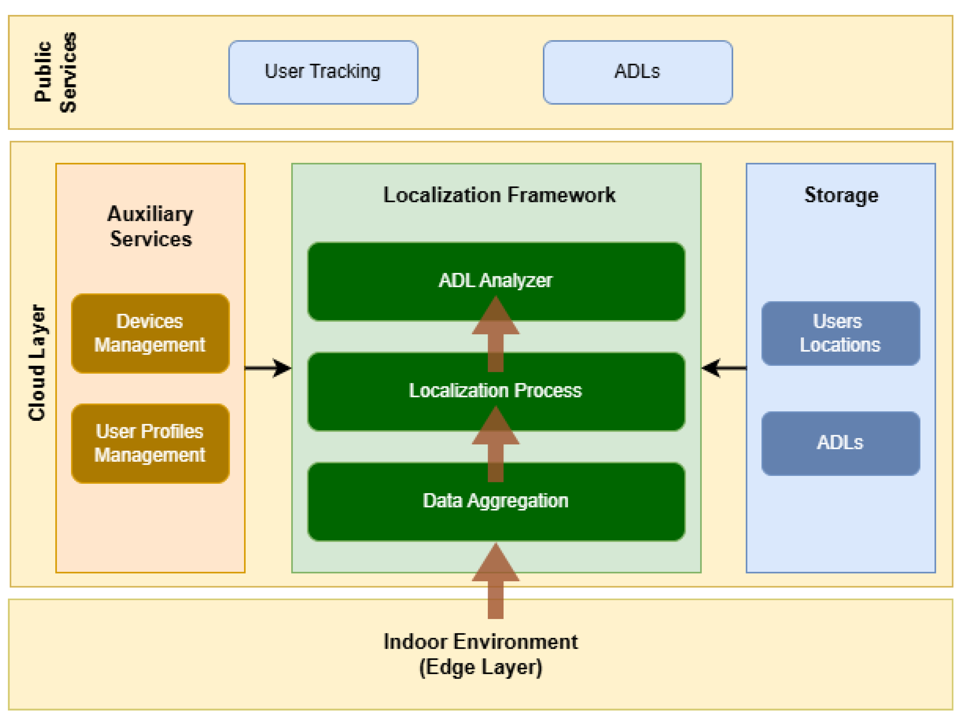
Figure 2.
Localization Process.
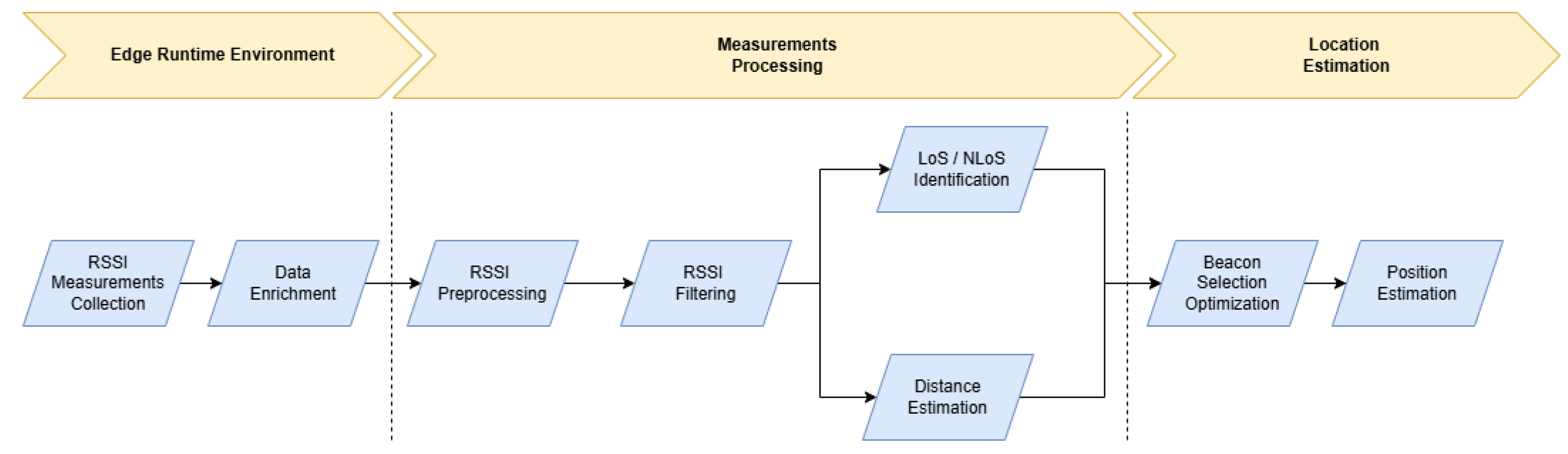
Figure 3.
RSSI Subset selection.
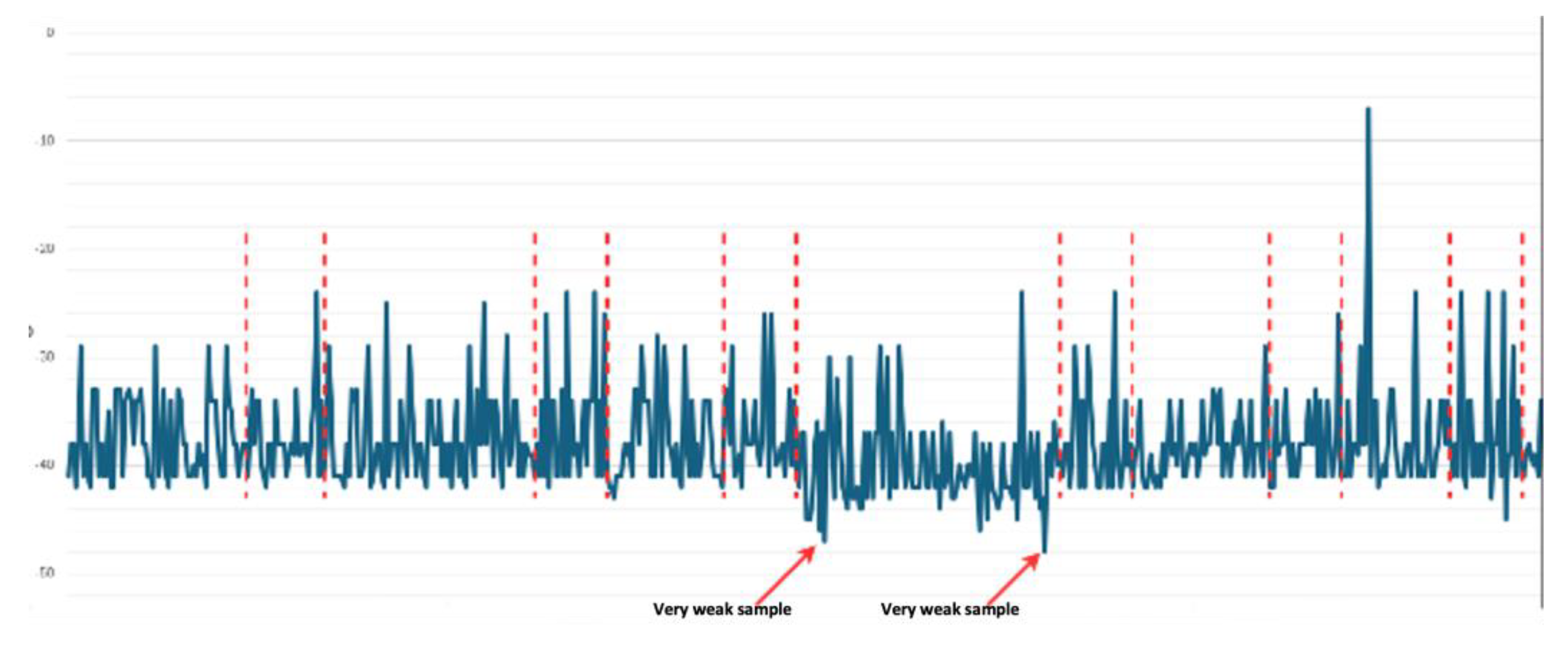
Figure 4.
RSSI Pre-processing results per scenario.
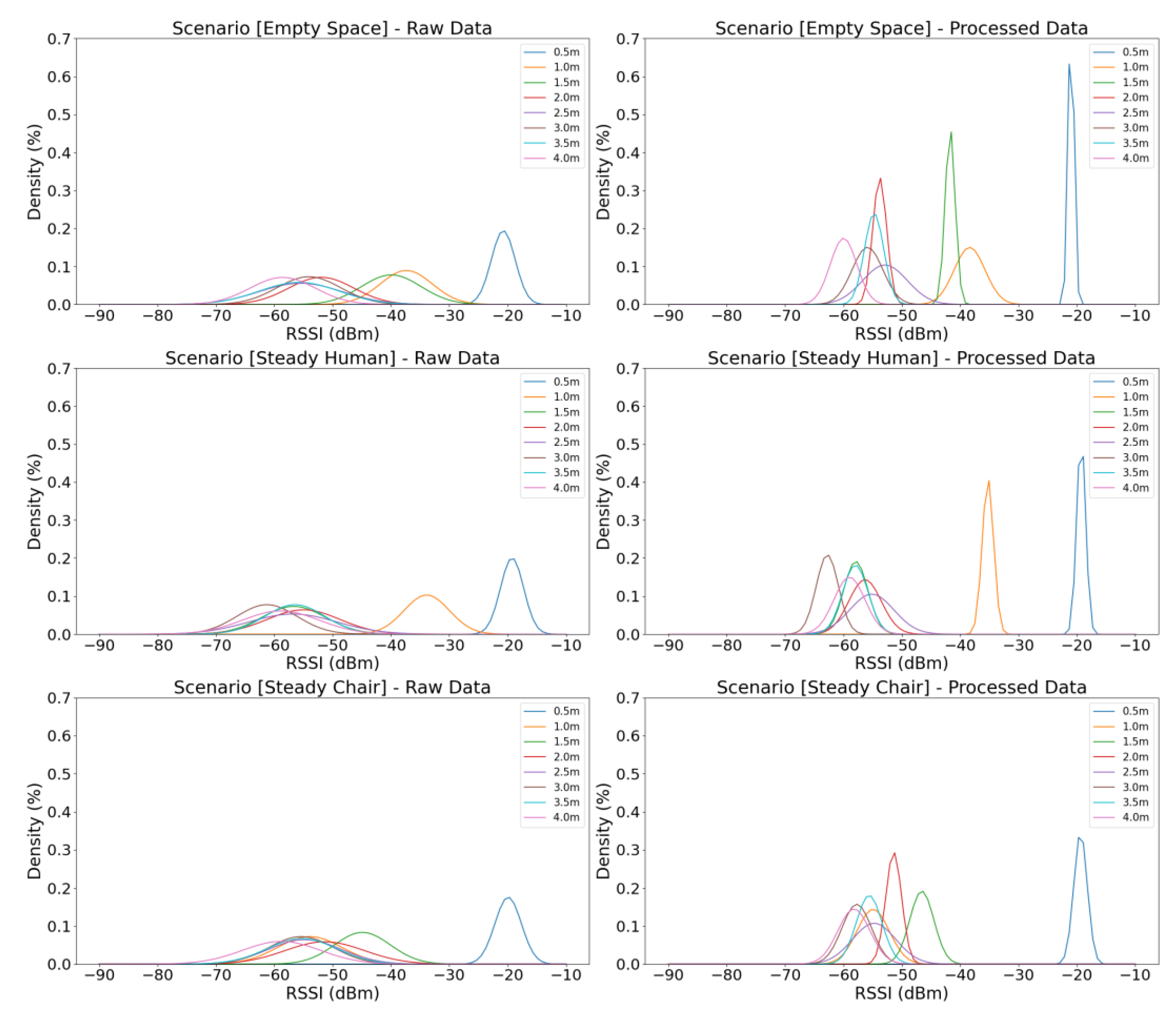
Figure 5.
Data Enrichment Process.
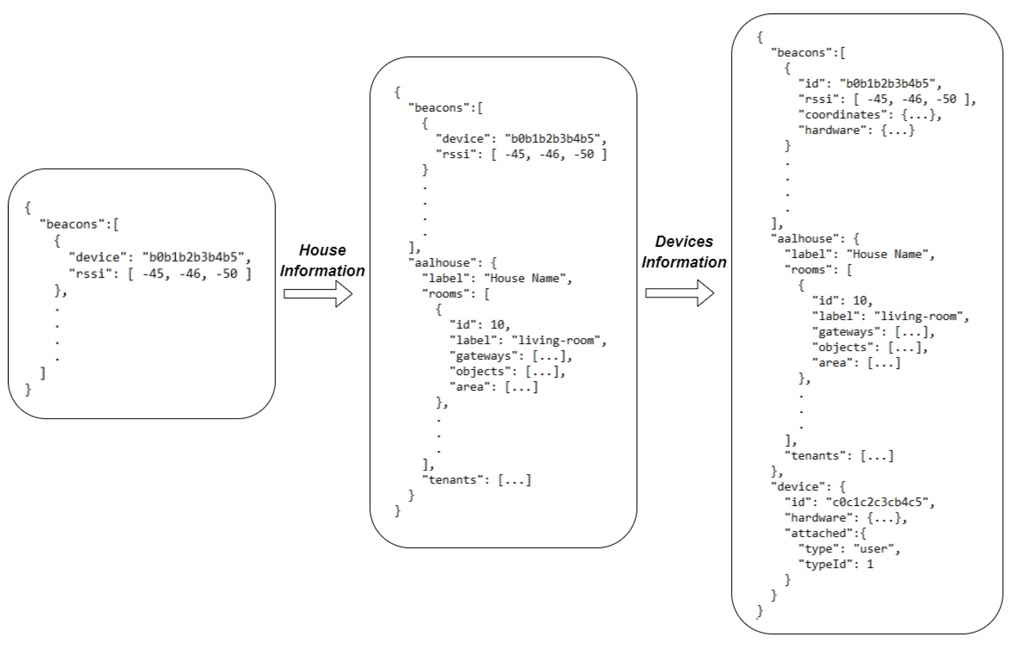
Figure 6.
Roc diagram for LoS/NLoS classification.

Figure 7.
Comparison Machine Learning diagram.
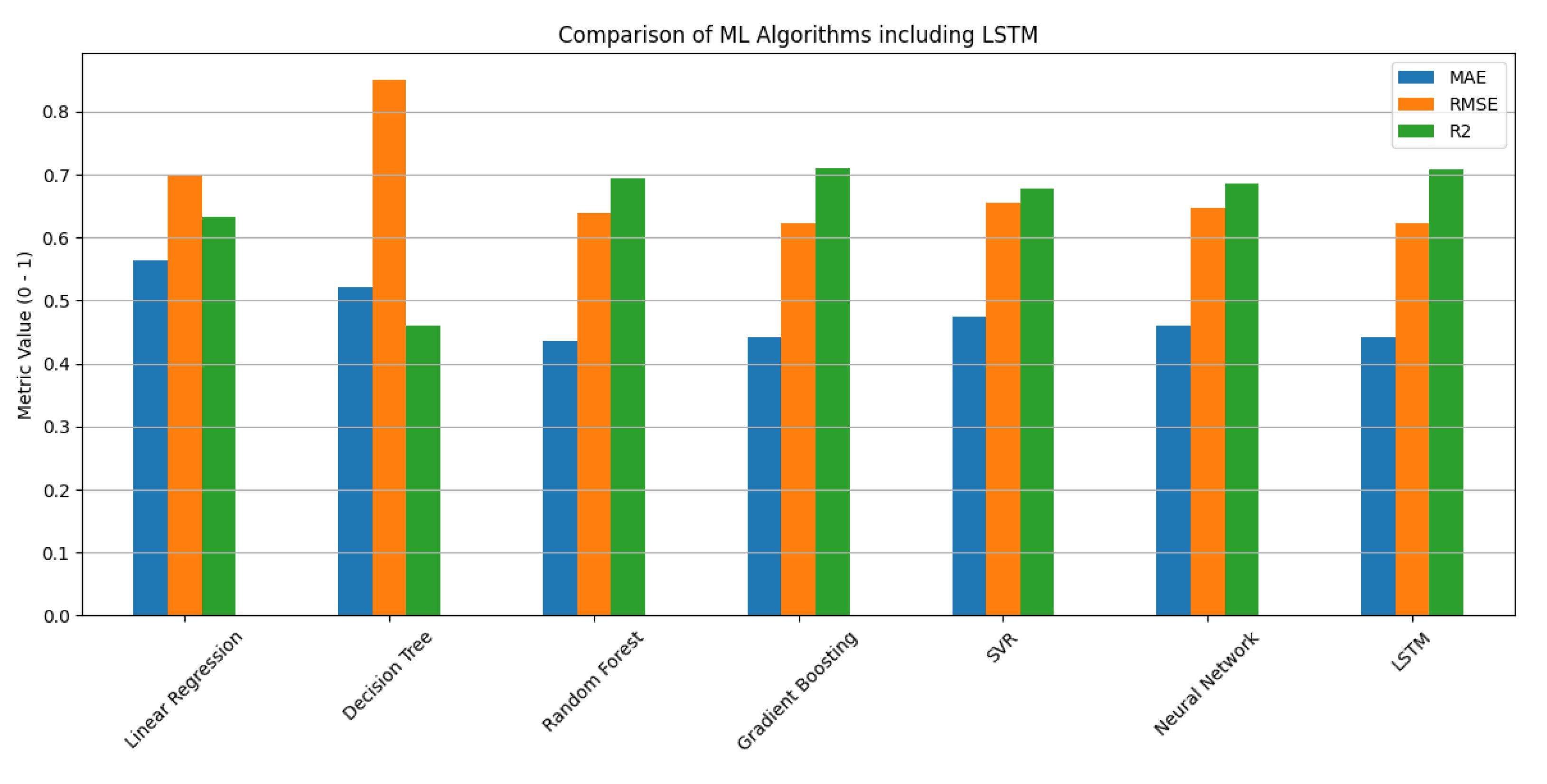
Figure 8.
Scenario visualization.
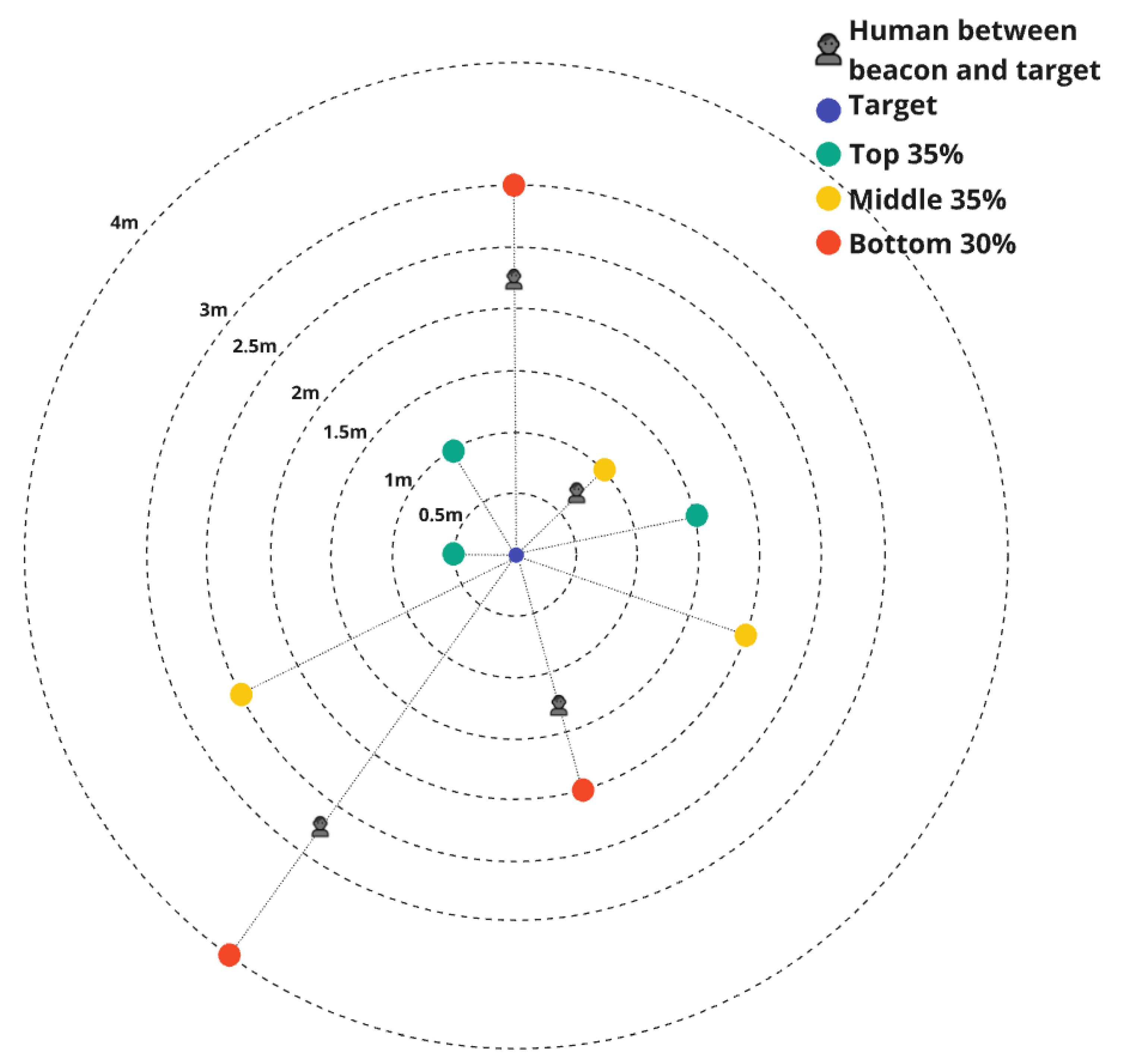
Figure 9.
Localization Process - Evaluation Setup (AAL).
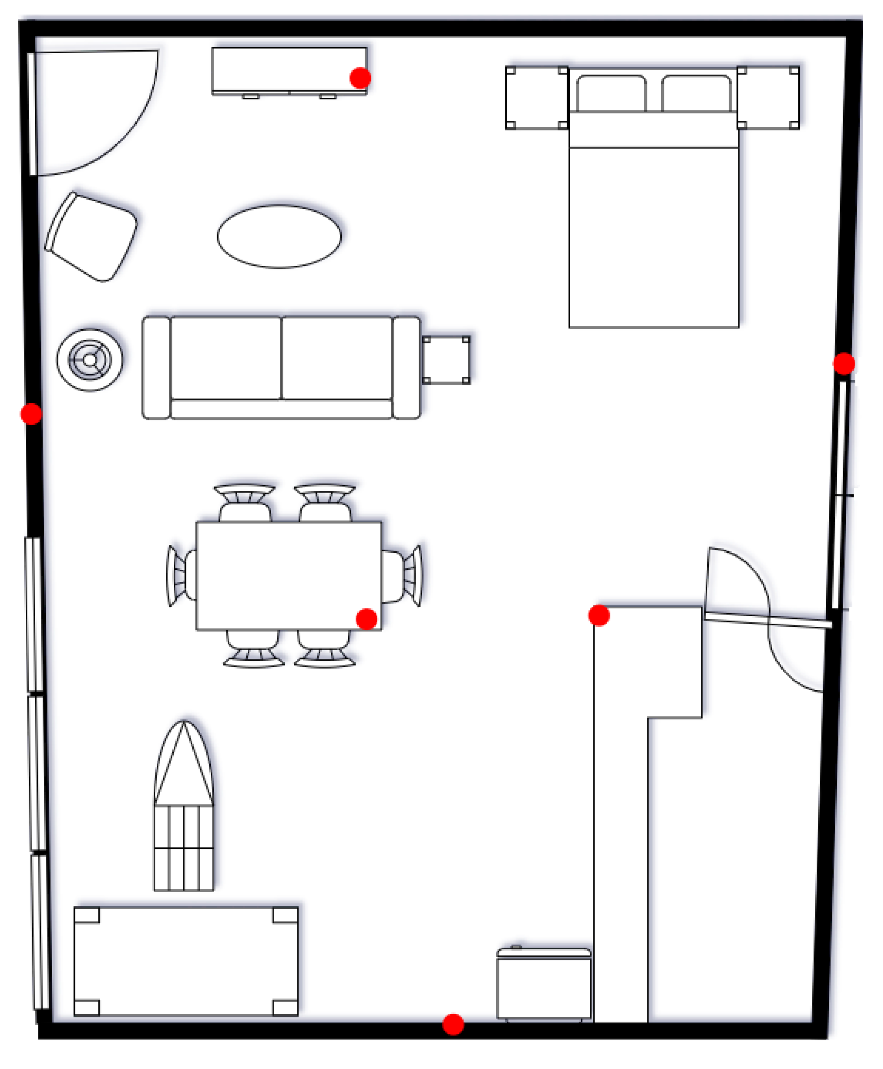
Figure 10.
Comparison of the 3 filters.
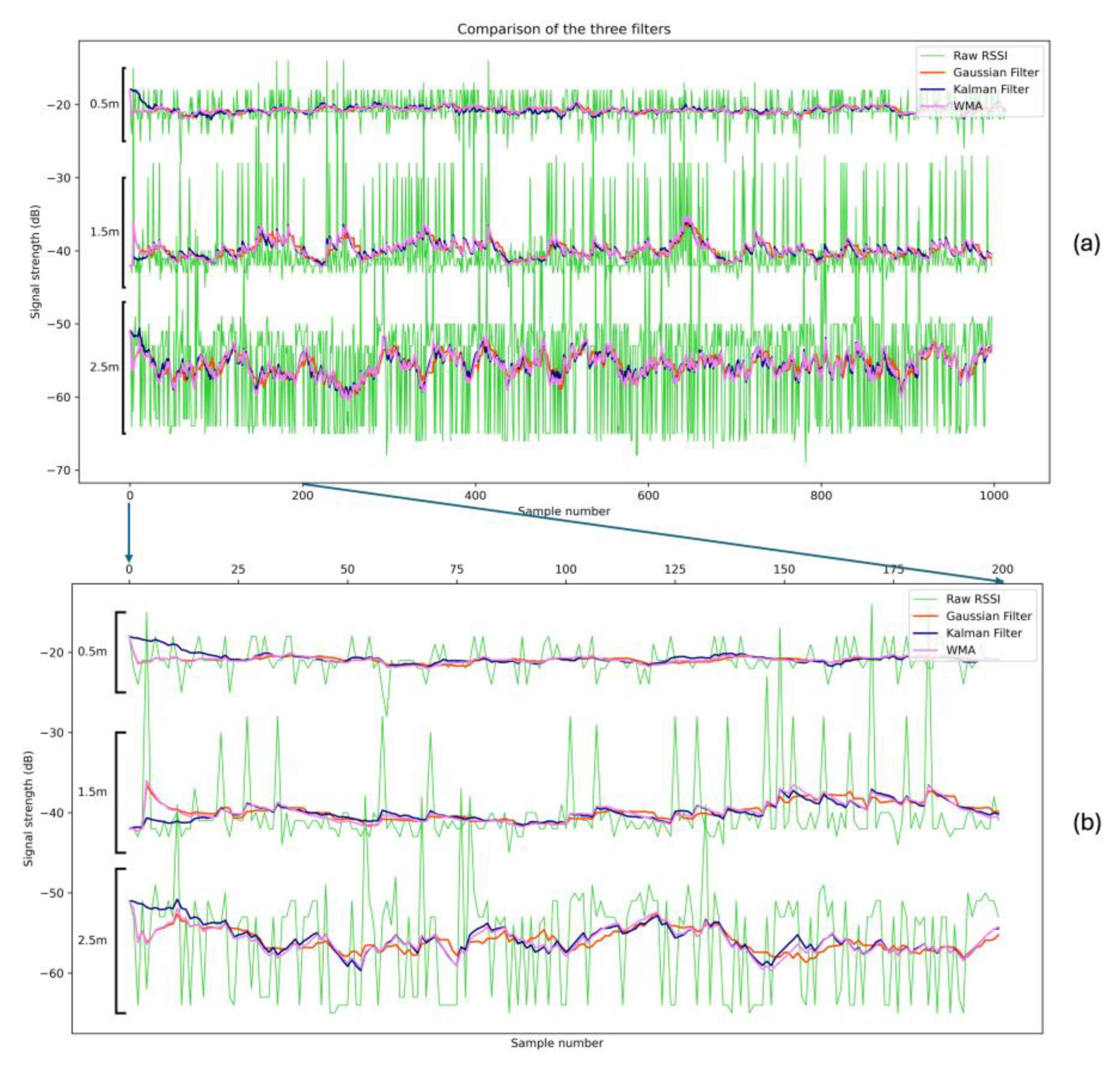
Figure 11.
Location Routes Evaluation.
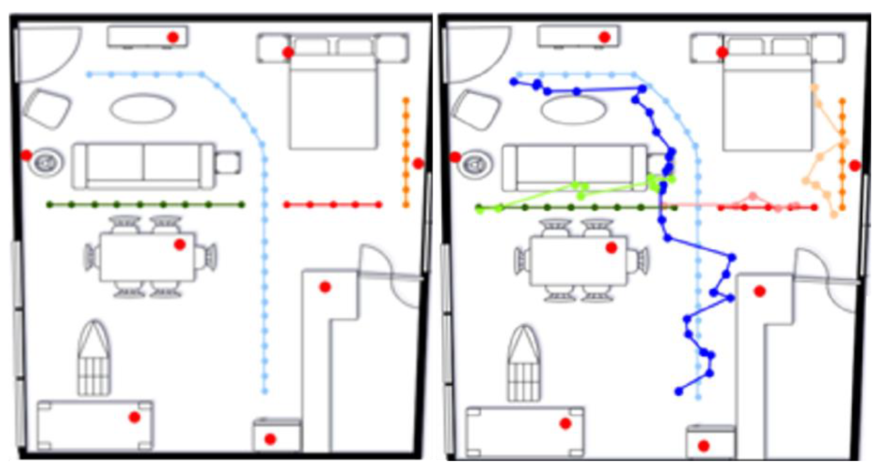
Figure 12.
Location Estimation Results.
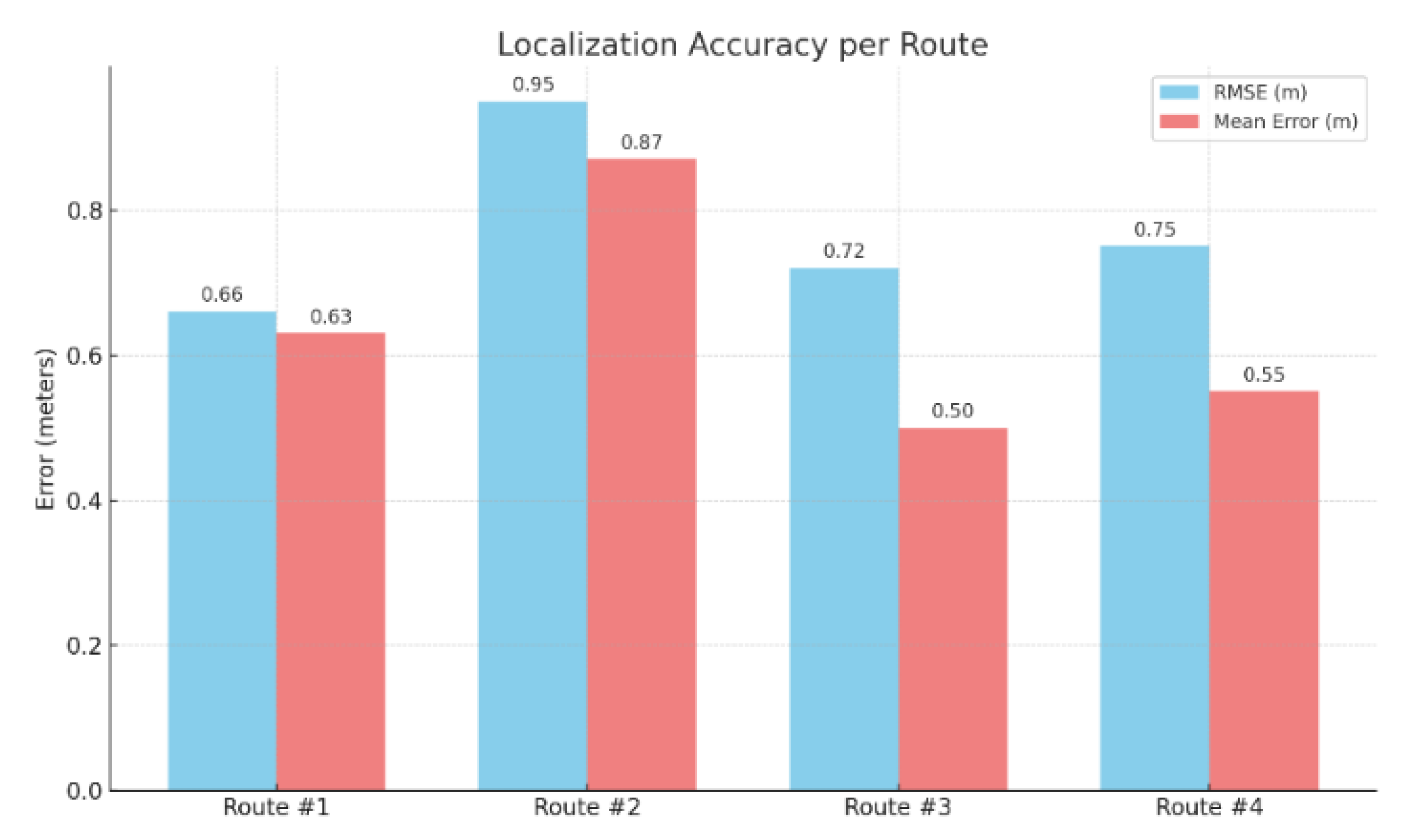
Figure 13.
User Paths Visualization.
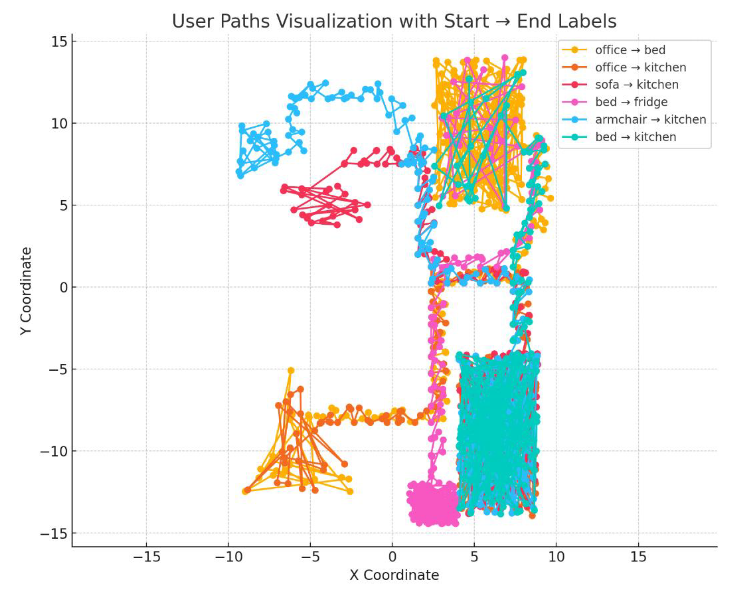
Figure 14.
Confusion matrix.
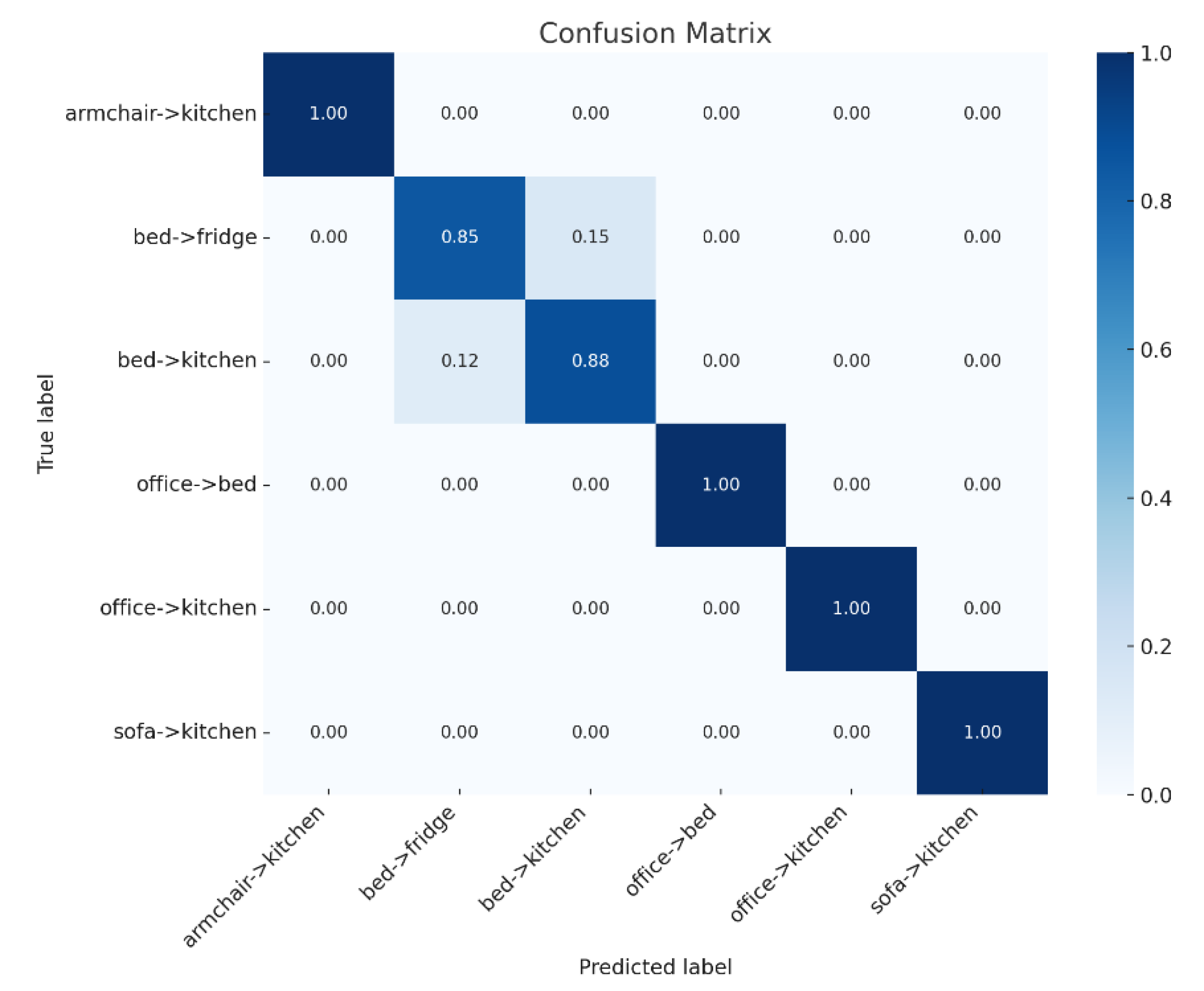
Figure 15.
User Paths Visualization.
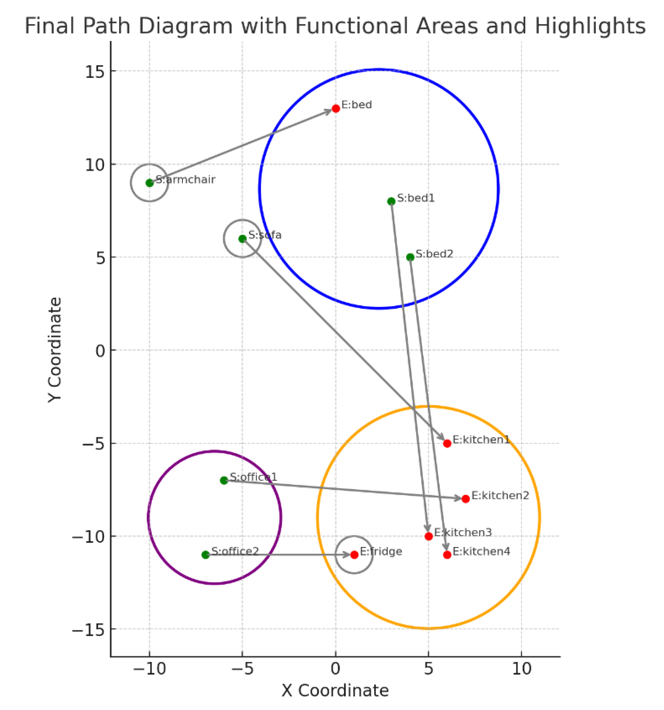

Table 1.
Rating Algorithm Weights.
| Criterion | Weight |
|---|---|
| Standard Deviation | 60% |
| RSSI Chunk Length | 20% |
| Loss Rate | 10% |
| Filtered Data Length | 10% |
Table 2.
Comparative table of Machine Learning algorithms.
| Model | Accuracy | Precision | Recall | F1-Score | Weight |
|---|---|---|---|---|---|
| Random Forest | 0.834 | 0.867 | 0.849 | 0.858 | 60% |
| k-Nearest Neighbors (kNN) | 0.813 | 0.848 | 0.833 | 0.840 | 20% |
| Support Vector Machine (SVM) | 0.705 | 0.686 | 0.923 | 0.787 | 10% |
| Neural Network | 0.722 | 0.736 | 0.826 | 0.778 | 10% |
Table 3.
Comparative table of Machine Learning algorithms.
| Name | Description | Involvement Ratio |
|---|---|---|
| Line of Sight | Beacons with a direct LoS to the receiver generally provide more stable RSSI readings. | 0.20 |
| RSSI Strength Score | Beacons are scored based on their mean RSSI value. It utilizes the raw signal. | 0.25 |
| Distance | Beacons that are estimated to be closer to the target get a higher score, as they provide more reliable signals. | 0.2 |
| RSSI Variance Score | Lower signal variance is preferred, as high fluctuations indicate instability. It is calculated based on the raw signal. | 0.1 |
| Entropy Score | This method quantifies the entropy of a beacon’s RSSI distribution, favoring beacons that provide more distinctive signal patterns useful for localization. It is calculated based on the raw signal. | 0.15 |
| Loss Rate | The loss rate is computed based on the number of missing packets in a given time window. It utilizes the raw signal. | 0.1 |
Table 4.
Learning algorithms MSE and variance at different distances.
| Kalman | WMA | Gaussian | ||||
| MSE (m2) | Variance | MSE(m2) | Variance | MSE(m2) | Variance | |
| 0.5m | 3.50 ⋅ 10-3 | 2 ⋅ 10-4 | 3.40 ⋅ 10-3 | 1 ⋅ 10-4 | 3.40 ⋅ 10-3 | 1 ⋅ 10-4 |
| 1.5m | 4.57 ⋅ 10-2 | 6.84 ⋅ 10-3 | 4.83 ⋅ 10-2 | 7.4 ⋅ 10-3 | 4.73 ⋅ 10-2 | 6.1 ⋅ 10-3 |
| 2.5m | 5.08 ⋅ 10-1 | 8.31 ⋅ 10-2 | 5.17 ⋅ 10-1 | 8.96 ⋅ 10-2 | 4.90 ⋅ 10-1 | 6.75 ⋅ 10-2 |
| Mean | 1.84 ⋅ 10-1 | 3.02 ⋅ 10-2 | 1.89 ⋅ 10-1 | 3.24 ⋅ 10-2 | 1.8 ⋅ 10-1 | 6.46 ⋅ 10-2 |
Table 5.
Model Comparison for LoS/NLoS classification.
| Model | MAE (m) | MSE (m2) | RMSE (m) | R² | MAPE (%) | MedAE (m) | Variance |
|---|---|---|---|---|---|---|---|
| Linear Regression | 0,72 | 0,80 | 0,89 | 0,38 | 45,56% | 0,62 | 0,38 |
| Random Forest Regressor | 0,50 | 0,57 | 0,76 | 0,56 | 30,14% | 0,30 | 0,56 |
| Support Vector Regressor | 0,59 | 0,66 | 0,81 | 0,48 | 33,84% | 0,44 | 0,49 |
| K-Nearest Neighbors Regressor | 0,50 | 0,57 | 0,76 | 0,56 | 30.74% | 0,30 | 0,56 |
| Gradient Boosting Regressor | 0,55 | 0,56 | 0,75 | 0,56 | 34,07% | 0,42 | 0,56 |
Table 6.
ADLs and their location in indoors environments.
| Room | ADLs |
|---|---|
| Kitchen | Cooking, eating, cleaning |
| Living room | Watching TV, sitting, resting |
| Bathroom | Showering, washing hands |
| Bedroom | Sleeping, dressing |
Table 7.
ADLs description.
| ADL | Location | Feature Extraction | Machine Learning |
|---|---|---|---|
| Cooking | Kitchen | Time spent in the kitchen, speed of movement, and transitions between the refrigerator, stove, and sink. | Classify the activity as cooking based on patterns of movement and time spent in the kitchen. |
| Resting / Sitting | Living room | Duration of stillness in a specific area, no movement or low movement for an extended period. | Recognize this activity by identifying prolonged stays in the living room with minimal movement. |
| Sleeping | Bedroom | Long periods of inactivity, detection of the person lying down, and absence of transitions. | Classify the activity as sleeping on long periods in the bedroom with little to no movement. |
Table 8.
Partial Predictions.
| Bed to kitchen Partial Prediction | Office to bed Partial Prediction | ||
|---|---|---|---|
| Destination | Probability (%) | Destination | Probability (%) |
| Bed -> kitchen | 99.82 | office -> bed | 75.11 |
| bed -> fridge | 0.17 | bed -> kitchen | 16.45 |
| office -> bed | 0.01 | armchair -> kitchen | 4.28 |
Disclaimer/Publisher’s Note: The statements, opinions and data contained in all publications are solely those of the individual author(s) and contributor(s) and not of MDPI and/or the editor(s). MDPI and/or the editor(s) disclaim responsibility for any injury to people or property resulting from any ideas, methods, instructions or products referred to in the content. |
© 2025 by the authors. Licensee MDPI, Basel, Switzerland. This article is an open access article distributed under the terms and conditions of the Creative Commons Attribution (CC BY) license (http://creativecommons.org/licenses/by/4.0/).
Copyright: This open access article is published under a Creative Commons CC BY 4.0 license, which permit the free download, distribution, and reuse, provided that the author and preprint are cited in any reuse.


