
Submitted:
27 May 2025
Posted:
28 May 2025
You are already at the latest version
Abstract
With the rapid development of the low-altitude economy and smart logistics, unmanned aerial vehicles (UAVs), as core low-altitude platforms, have been widely applied in urban delivery, emergency rescue, and other fields. Although path planning in complex environments has become a research hotspot, optimization and scheduling of UAVs under time window constraints and task assignments remain insufficiently studied. To address this issue, this paper proposes an improved algorithmic framework based on a two-layer structure to enhance the intelligence and coordination efficiency of multi-UAV path planning. In the lower-layer path planning stage, considering the limitations of the Whale Optimization Algorithm (WOA) such as slow convergence, low precision, and susceptibility to local optima, this study integrates a backward learning mechanism, nonlinear convergence factor, random number generation strategy, and genetic algorithm principle to construct an improved IWOA. These enhancements significantly strengthen the global search capability and convergence performance of the algorithm. In the upper-layer task assignment stage, in response to the tendency of the Adaptive Large Neighborhood Search (ALNS) algorithm to fall into local optima under complex constraints, we incorporate K-means clustering for initialization and a simulated annealing mechanism, thereby proposing an improved IALNS to enhance scheduling rationality and solution efficiency. Through the coordination between the upper and lower layers, the overall solution flexibility is improved. Experimental results demonstrate that the proposed IALNS-IWOA two-layer method outperforms the conventional IALNS-WOA approach by 7.30% in solution quality and 7.36% in environmental adaptability, effectively improving the overall performance of UAV trajectory planning.
Keywords:
trajectory planning
; time window
; task allocation
; two-layer structure
; improved whale optimization algorithm
1. Introduction
The Outline of the Strategic Plan for Expanding Domestic Demand (2022–2035), issued by the Central Committee of the Communist Party of China and the State Council, explicitly proposes “supporting the application of technologies such as autonomous driving and unmanned delivery”, highlighting the development of new types of consumption. This marks the formal entry of the low-altitude economy into industrialization and standardization [1]. Low-altitude airspace policies are being continuously refined, and low-altitude aircraft technologies are rapidly advancing. As a result, drone applications in low-altitude airspace have expanded, particularly in military reconnaissance, emergency rescue, and logistics delivery applications [2]. However, traditional single-drone models can no longer meet the demands of large-scale applications. Ensuring the safety, feasibility, and optimality of multi-drone cooperative flight paths under multiple constraints has become a core challenge in the field of intelligent path planning.
The drone task assignment problem with time windows can be abstracted as a dynamic scheduling problem involving multiple agents under spatiotemporal constraints. Essentially, it is an extension of the Vehicle Routing Problem with Time Windows (VRP-TW) [3]. With ongoing technological advancements, research on VRP-TW has become increasingly diversified, ranging from traditional single-depot route planning to more complex scenarios involving multiple depots and time window constraints. The literature [4] developed an adaptive genetic algorithm with dynamic crossover/mutation probabilities, enhancing solution efficiency and quality. The literature [5] used an LSTM network to predict logistics demands, integrating forecasts into VRP for routing optimization. For problems involving hard time windows and heterogeneous vehicle types, BPC model with capacity inequalities to reduce the relaxation gap was introduced to improve urban waste collection efficiency successfully [6]. The literature [7] developed a novel mathematical model using an innovative backtracking approach to address a variable-location delivery problem with multiple time windows, using hospital data to assess the impact of delivery locations and cost functions, thereby enhancing delivery flexibility. The literature [8] recognized the need for dynamic route adjustments in emergency rescue scenarios, and argued that soft time windows are more appropriate. Mathematical model for optimizing multi-rescue-vehicle routes with soft time windows for a multi-depot scenario is constructed and a hybrid genetic algorithm incorporating a nearest-neighbor heuristic to solve the problem is proposed. While VRP and its variants have been widely studied—particularly in optimizing multi-depot vehicle scheduling to reduce logistics costs and enhance transportation efficiency, research on applying VRP to drone systems has lagged. With the rapid development of drone technologies, more researchers are now beginning to apply VRP methodologies to drone path planning. Unlike traditional vehicle delivery problems, drone routing must consider additional physical constraints such as ground obstacles, flight altitude, and range limitations, as well as aerial no-fly zones, payload capacities, and multi-drone coordination.
In recent years, with the rapid development of deep learning and distributed control technology, multi-UAV formation path planning and scheduling has become a research hotspot. The literature [9] achieved dynamic obstacle avoidance and cooperative formation in complex urban environments by using deep reinforcement learning methods, which significantly improved the planning efficiency and robustness. The literature [10] proposed a hybrid algorithm combining genetic algorithm and particle swarm optimization for real-time multi-UAV task scheduling and achieved better performance in scenarios containing hard and soft time window constraints. In addition, the literature [11] proposed a distributed consensus-based coordination strategy for heterogeneous UAV formations, which effectively mitigates the cooperative degradation problem when the communication bandwidth is limited. However, most of the above works focus on single-layer path or scheduling optimization, failing to simultaneously consider the coupled optimization of path planning and task allocation under spatio-temporal constraints. The literature [12] proposed a hybrid distributed scheduling framework based on deep reinforcement learning to cope with the dynamic task allocation problem in urban disaster relief; The literature [13] introduced a path prediction algorithm based on graph neural networks in a multi-UAV collaborative environment, realizing real-time obstacle avoidance in dense urban airspace; The literature [14] optimized airspace sharing and game theory among different operators by combining multi-intelligent reinforcement learning and game theory. real-time obstacle avoidance in high-density urban airspace. Whereas these studies show significant differences in algorithm design, simulation scenarios, and application focus in different regions, they all face the challenge of trade-off between coordination efficiency and real-time performance. There is a lack of a unified evaluation framework to compare the performance of different methods in multiple typical scenarios, which is difficult to guide practical system deployment.
Based on these gaps this paper proposes a two-layer algorithmic framework from three perspectives of 3D modeling, spatio-temporal constraints and task allocation to achieve algorithmic generalization and superior performance across scenarios. Therefore, to address the problems of inefficient coupling of task assignment and path optimization, easy to fall into local optimum, and insufficient consideration of multi-dimensional constraints such as time window, load, range and terrain in existing multi-UAV scheduling algorithms under spatio-temporal constraints, this paper proposes a two-layer structure-based IALNS-IWOA cooperative framework. In the upper-level task allocation stage, the Improved Adaptive Large Neighborhood Search (IALNS) introduces K-means clustering to construct the initial solution and combines the simulated annealing acceptance criterion in order to enhance the diversity of the solutions and the ability of jumping out of the local optimums; in the lower-level path planning stage, the Improved Whale Optimization Algorithm (IWOA) strengthens global search through an adversarial learning mechanism with nonlinear convergence factors, and embeds a genetic operator to achieve the global search, and embeds a genetic algorithm to achieve the global search. search, and embedded genetic operators to achieve local variation to enhance the solution accuracy; the two interact with each other through iterative information, with the upper-layer allocation results guiding the lower-layer planning and the lower-layer cost feeding back to the upper-layer update, thus achieving efficient collaborative scheduling and a significant improvement in optimization performance in a multi-UAV multi-constraint environment.
2. Modeling
The Multi-Drone Routing Problem with Time Windows (MDRP-TW) extends the classical Vehicle Routing Problem with Time Windows (VRP-TW) to multiple aerial vehicles operating in 3D space. In MDRP-TW, a fleet of UAVs must service spatially distributed tasks—each with its own time window and demand—while respecting additional aerial constraints such as altitude limits, no-fly zones, endurance and payload capacities. The objective is to jointly assign tasks to drones and generate collision-free, energy-efficient 3D trajectories that minimize a composite cost (e.g. time, distance, or energy) under these spatio-temporal constraints. To ensure the alignment of the planned routing scheme with real-world application scenarios while maintaining feasibility and effectiveness, it is necessary to establish constraint conditions for the MDRP-TW model. This section provides the mathematical formulation of the Multi-Drone Routing Problem with Time Window (MDRP-TW). The model incorporates various real-world constraints such as no-fly zones, altitude restrictions, time windows, and UAV payload capabilities. The objective functions are detailed in Equations (1) through (5).
Here, in Equation 1 represents the objective function of the MDRP-TW model, denotes the objective function of the task allocation model, and represents the objective function of the trajectory optimization model. Specifically. in Equation 2 denotes the cost associated with time window constraints, the cost related to payload constraints, denotes the weighting coefficient in the task allocation model. In Equation 3 the cost of trajectory length constraints with a weighting factor of , in addition, indicates the cost due to no-fly zone constraints with a weighting factor of , denotes the cost related to flight altitude constraints with a weighting factor of , refers to the cost of flight smoothness constraints with a weighting factor of , and represents the cost arising from spatial conflict constraints with a weighting factor of . and all weight coefficients add up to 1 in Equation 5, ensuring flexibility in problem adjustment. Table 1 defines all the mathematical symbols used in the model of this study and their meanings, while Figure 1 shows a schematic diagram of the no-fly zone model with the coordinates of the trajectory points and the coordinates of the centre axis of the no-fly zone, and distinguishes the meanings of different distances between the UAV and the no-fly zone.
In this study, the no-fly zone is modeled as an infinitely high cylinder. Let the coordinates of the trajectory point be denoted as , and a point on the central axis of the no-fly zone be denoted as .
2.1. Mathematical Model of the Trajectory Planning Layer
To solve the MDRP-TW problem, a dual-layer framework is constructed in this study. The drone flight path is represented by a set of discrete trajectory points, denoted as set . The first step is to determine the optimal trajectory between each pair of task points, which defines the trajectory optimization layer [15,16,17]. The specific formulation is provided in Equations (6) through (13).
All symbols in Equation 6 to Equation 13 are defined as before. The schematic of Eq. 13 is shown in Figure 2, which shows the UAV flying a distance over two different lines of operation.
Having modelled the assessment of each UAV trajectory based on spatial and safety constraints, the focus will now be on a tasking model that determines which UAV is assigned to which task point, considering the time window and payload constraints.
2.2. Mathematical Model of the Task Allocation Layer
Task allocation layer assigns tasks based on the information provided by the lower-level path planning model, considering time windows, task loads, and drone payload capacities. Let denote the total number of task points and represent the number of drones used. Task allocation is determined according to task loads. The specific formulations are given in Equations (14) to (16).
In this case, the constraints for both and are realized by imposing great penalties, which increase as the degree of constraint violation increases; the number of unoccupied people and the number of tasks is derived by back-calculating the number of tasks, which can vary with the number of tasks.
Having defined the mathematical formulation of the MDRP-TW problem, work will proceed to describe the solution strategy. A two-tier meta-heuristic algorithm - the IALNS algorithm for task assignments and the IWOA algorithm for path planning - is designed to solve the problem efficiently.
3. IALNS-IWOA Algorithm
Single-layer optimization methods are often insufficient for MDRP-TW problems, as they cannot simultaneously handle spatial-temporal trajectory constraints and combinatorial task assignment. Therefore, a hierarchical framework is adopted, where the upper layer handles assignment feasibility, and the lower layer focuses on trajectory cost minimization. The dual-layer architecture adopted in this study offers distinct structural advantages, as it decouples the task allocation and path optimization processes, thereby providing greater flexibility and scalability when addressing complex constraint problems. First, an improved Whale Optimization Algorithm (IWOA) is employed to plan the optimal flight path between each pair of task points. Then, an Improved Adaptive Large Neighborhood Search algorithm (IALNS) is used to optimize task allocation by determining the visiting sequence of task points for each drone. This approach reduces conflicts and idle time during the task assignment process, thereby improving the overall efficiency of multi-drone cooperative operations. IALNS and IWOA each possess unique optimization capabilities: the former demonstrates strong local search performance in solving combinatorial optimization problems [18], while the latter offers superior global search ability, effectively avoiding entrapment in local optima [19]. The overall dual-layer architecture of the proposed framework is illustrated in Figure 3.
A two-tier solution framework is designed based on the MDRP-TW mathematical formulation in Section 2. The lower layer focuses on optimal trajectory generation between task points, while the upper layer determines the distribution of these tasks among available UAVs. Starting with the trajectory planning part.
3.1. Adaptive Large Neighborhood Search
The Adaptive Large Neighborhood Search (ALNS) algorithm [20] has been widely applied to complex combinatorial optimization problems. Its core idea is to iteratively perform destruction-repair operations to evolve the solution. Traditional ALNS generates an initial solution and treats it as the current best solution. During the iterative process, new solutions are produced through destruction and repair operators and are accepted based on a roulette-wheel mechanism, continuing until the maximum number of iterations is reached or other termination criteria are satisfied. However, such an initialization is prone to falling into local optima and is difficult to escape. Moreover, the operator selection and weight adjustment mechanisms lack adaptability, resulting in low computational efficiency, especially for large-scale problems. To address these issues, this study incorporates a K-means clustering strategy [21] during the algorithm initialization phase. During the solution update stage, simulated annealing is employed to determine whether the new solution should be accepted within the IALNS framework. The algorithm flow is illustrated in Figure 4.
3.1.1. K-Means Clustering
The K-Means clustering method divides the given dataset into different clusters such that the data points in the same cluster show high similarity and the data point information is shown in Table 5, while the data points in different clusters have relatively low similarity [22]. The core idea is to iteratively search for cluster centers such that the sum of distances from each data point to the center of its assigned cluster is minimized. In this study, the number of clusters is set equal to the number of drones deployed. The clustering formulation for K-Means is shown in Equation (17).
Here, denotes the cluster, the mathematical meaning of which is the sum of the squares of the errors within the cluster, and represents a data point belonging to cluster . During the iterative optimization process, the cluster centers are continuously updated to gradually reduce the objective function value until convergence is achieved. The use of K-Means clustering during initialization enables the generation of solutions with better structure and rationality, facilitating faster convergence of the algorithm toward near-optimal solutions. The clustering results are shown in Figure 5, where the three coloured task points shown are the initial solution classifications.
3.1.2. Simulated Annealing Algorithm
Simulated Annealing (SA) is a general probabilistic algorithm commonly used to search for the global optimum within a large solution space [23]. Its core lies in the acceptance criterion, which is defined in Equation (18).
Here, represents the probability of accepting a new solution, is the difference in objective function value between the new solution and the current solution, and denotes the current temperature. The ALNS algorithm is prone to becoming trapped in local optima during the search process. To address this, IALNS integrates the concept of simulated annealing, allowing the algorithm to probabilistically accept inferior solutions under certain conditions. This facilitates escape from local optima, broadens the search space, and increases the likelihood of finding a global optimum. In summary, the pseudocode of IALNS is presented in Table 2.
While the IWOA module provides high-quality inter-point trajectory costs, it requires an effective upper-layer strategy to assign tasks to UAVs. We thus construct an Improved Adaptive Large Neighborhood Search (IALNS) framework to explore the assignment space under multiple constraints.
3.2. Improved Whale Optimization Algorithm
The Whale Optimization Algorithm (WOA) is a swarm intelligence optimization algorithm inspired by the foraging behavior of humpback whales, and it has been widely applied to solve nonlinear optimization problems. However, WOA tends to fall into local optima, has limited global search capability, and struggles with complex constraint scenarios. To address these issues, this study introduces reverse learning mechanisms, nonlinear convergence factors, random number generation strategy, and evolutionary algorithm techniques to propose an Improved Whale Optimization Algorithm (IWOA) for optimizing drone trajectory planning. Reverse learning enhances the diversity of the initial population, while the convergence factor is modified from linear to nonlinear decay. Additionally, enhanced random number generation mechanism is integrated into the iteration process to coordinate the algorithm’s global exploration and local exploitation capabilities [24]. The flowchart of the proposed IWOA is shown in Figure 6.
3.2.1. Simulated Annealing Algorithm
The core of the Genetic Algorithm (GA) lies in crossover and mutation operations. By applying these operations to parent individuals, GA generates offspring and searches for the solution space to find better solutions. In this study, solution updates are guided by this principle: a new solution is generated by comparing the current solution with another solution produced through crossover and mutation, and the better one is selected as the optimal solution for the current generation [25]. The crossover operation simulates genetic information exchange between two individuals. The corresponding formulations are shown in Equations (19) and (20).
Here, and represent the parent individuals, denotes the offspring individual, is the crossover coefficient, is the crossover control parameter, and is a binary variable used to control crossover directionality.
The mutation operation is applied to adjust individuals after crossover, helping to prevent premature convergence to local optima. Based on a multipoint mutation strategy, the mutation update is formulated as shown in Equation (21).
Here, denotes the value of the decision variable of the current individual, and represents the value of the decision variable after mutation. and are the allowable maximum and minimum values of the normalized decision variable. and represent the distances between the current solution and the upper and lower bounds, respectively. In summary, the pseudocode for the Improved Whale Optimization Algorithm (IWOA) is provided in Table 3.
This chapter outlines the overall algorithmic structure. The IWOA and IALNS components of architecture operate in a coordinated manner, with IWOA providing the trajectory costs of the task combinations, and IALNS using this information to adaptively re-assign tasks. The interplay between these two layers enables flexible yet coordinated optimization. In the following section, we validate the proposed method through simulation experiments under various mission settings.
4. Simulation Experiments
4.1. Simulation Environment and Mapping to Mathematical Model
To ensure that the proposed mathematical model is faithfully reflected in the simulation environment, this section presents a structured mapping from the model components to their implementation in MATLAB. with the simulation environment set as a 3D space of size , containing 2 no-fly zones, 1 starting point, and 15 task points with varying task loads. The maximum payload capacity of a single drone was set to 110 [26]. Using the Analytic Hierarchy Process (AHP) [27], and after consistency verification, the weight coefficients were determined as follows: ; , , , , were set to 0.4357, 0.1875, 0.0625, 0.2500, and 0.0625, respectively. In the simulation code, these are used as fixed input parameters during fitness evaluation. As illustrated in Figure 7, the terrain environment was modeled in 3D space using curved surfaces and cylindrical volumes to simulate obstacles and topographical constraints. The information from this map will be used as input for the lower trajectory planning section. These elements were considered infinitely high and impassable. The corresponding data are listed in Table 4:
The distribution of task points in the terrain is shown in Figure 8, Figure 7 and Table 4 reflect the inputs to the lower objective function . The mentioned in Equation (3) uses the distance between the UAV path and the no-fly zone, and the calculates the spacing between the UAVs to avoid conflicts. penalizes flights that exceed the allowable flight altitude range, and Each term shown in the representation is a method for calculating the flight altitude range. And the symbols , , represent that each term shown is calculated based on the 3D environment and geometry using equations (6)-(13).
The mission point information is shown in Table 5, complete with a mapping of the upper-level objective function . Where is the penalty for violating the time window as shown in Eq. (14), which is computed by comparing the arrival time of each mission point with its allowed service interval. represents the mission overload as shown in Equation (15), which penalizes the UAV if its total mission exceeds the payload limit. These values are calculated during the mission assignment phase using time and load data extracted from the solution.
Figure 8 shows the spatial distribution of the mission points in the side and top views. These mission locations are represented as basic inputs to the mission assignment framework defined in Equations (1)-(3), where UAVs are assigned based on their spatio-temporal distance and capacity constraints.
The total objective function is shown in Equation (1), where denotes the mission assignment cost and denotes the trajectory cost. In the simulation, the environmental parameters are transformed into a model for input, using IALNS algorithm to calculate , using IWOA to calculate , and finally adjusting the weights by AHP to output . The specific process is shown in Figure 9.
4.2. Experimental Results
4.2.1. Algorithm Base Performance Validation
In order to validate the effectiveness of the proposed IWOA, this study compares the IWOA with the WOA, PSO and ACO using five benchmark test functions as shown in Table 6. Among them, - are unimodal test functions, is multimodal test function, and are fixed-dimension multimodal test functions. Each algorithm was run for 100 iterations. The average value and standard deviation of the results were used as evaluation metrics. Detailed test functions are listed in Table 7.
As shown in Table 7, based on the comparison of mean values and standard deviations of the optimal search results, IWOA exhibits slightly lower search precision than PSO only for the test function. However, for the other test functions, the optimal and mean values obtained by IWOA are smaller than those of the other algorithms. Moreover, IWOA achieves theoretical optimal values in the and tests, demonstrating that the improved algorithm is more stable.
Table 7 shows that IWOA reaches the theoretical optimal value in single-peak function and fixed-dimension multi-peak function with lower standard deviation than traditional algorithms, which proves that it has the stability and anti-local optimality in complex optimization problems, and provides the algorithmic basis for UAV trajectory optimization.
4.2.2. Simulated Annealing Algorithm
The number of drones used is set to three. The algorithms compared include IALNS-IWOA, IALNS-WOA, IALNS-PSO, and IALNS-ACO, each with an average population size of 90 and a maximum number of 300 generations. Multi-drone cooperative path planning based on the dual-layer algorithm was simulated, and the experimental results are shown in Figure 9, Figure 10, Figure 11 and Figure 12.
The fitness value represents the total cost of combining the task assignment penalty and the trajectory planning objective. As shown in Figure 13, the proposed IALNS-IWOA algorithm converges the fastest and has the lowest final fitness value. All algorithms exhibit exploration fluctuations during the first 50 iterations; however, IALNS-IWOA converge significantly earlier, i.e., around 120 iterations. The other algorithms either converge slowly or fluctuate around the local optimum. This performance improvement stems from the synergy of the two-layer architecture, where IWOA enhances global trajectory exploration using nonlinear convergence and adaptive mutation, while IALNS dynamically adjusts task allocation using adaptive damage-repair operators and simulated annealing. Together, they enable efficient navigation of large solution spaces and robust escape from local optima. The smoother convergence profile of IALNS-IWOA also reflects a better balance between exploration and exploitation, confirming its robustness and efficiency in solving MDRP-TW with complex constraints.
The visualization of the experimental results clearly demonstrates the superiority of IALNS-IWOA in solving trajectory planning for VRP-TW. Detailed information on the dual-layer structures of the different algorithms is presented in Table 8.
The comparison results indicate that the proposed dual-layer framework effectively addresses the multi-drone coordination problem with time windows. Specifically, the total fitness of the IALNS-IWOA model is 7.36% higher than that of the IALNS-WOA model, 3.08% higher than that of the IALNS-PSO model, and 39.13% higher than that of the IALNS-ACO model. In terms of total flight distance, the IALNS-IWOA model achieves reductions of 7.30%, 3.34%, and 16.43% compared to the IALNS-WOA, IALNS-PSO, and IALNS-ACO models, respectively. These results validate both the effectiveness of the improved algorithm and the superiority of the proposed dual-layer framework.
4.2.3. Extended Experiments Under Varying Mission Scenarios
To further evaluate the scalability, adaptability and robustness of the proposed IALNS-IWOA algorithm, the study conducted two additional simulation experiments under mission scenarios of varying complexity. These extended cases aim to validate the performance of the algorithm when varying the number of mission points, the presence of obstacles and the number of UAVs required. The generalized capabilities of the two-tier planning framework proposed in this paper are demonstrated by analyzing both lightly loaded scenarios and complex, obstacle-rich scenarios.
The lightweight experiment was conducted first, and in this minimal configuration, five mission points were randomly placed in a flat 3D environment with an area of 500 × 500 × 300. The mission point information is shown in Table V for mission points 1 to 5, with no terrain obstacles or no-fly zones. The payload and flight parameters of the UAV are consistent with the main experiment. The experimental environment is shown in Figure 14.
After task evaluation and trajectory planning, the algorithm assigns tasks to two UAVs. The planned trajectories are shown in Figure 15.
Among them, the flight trajectories generated by IALNS-IWOA are compact and spatially separated from each other, which ensures efficient mission coverage and minimal overlap. At this point the experiment yields an adaptation level of A. The mission information performed by each UAV is shown in Table 9.
The results of this experiment show that the IALNS-IWOA algorithm can efficiently determine balanced assignments and short and feasible flight paths without unnecessary complexity, even in the case of sparse tasks.
The second one is the complexity experiment, in which the complexity of the environment and the density of the tasks were increased. Twenty task points were randomly distributed in 3D space, except for task point 1-task point 15 shown in Table 5, the information of the added task points is shown in Table 10; meanwhile, three cylindrical no-fly zones were introduced to simulate the complex environment with dense obstacles, except for cylinder 1-cylinder 2 shown in Table 4, the information of the added cylinders is shown in Table 11. This experimental environment is shown in Figure 16.
The algorithm automatically calculates that four UAVs are required for optimal coverage due to the cumulative mission requirements and spatial complexity of the layout. The planning trajectory is shown in Figure 17. As can be seen from the figures, the trajectory avoids forbidden areas while maintaining reasonable distances and smooth transitions. The UAV task assignments, coverage task sequences, total distance flown, and final fitness values are detailed in Table 12. Despite the increased difficulty, the IALNS-IWOA framework maintains the feasibility of the trajectory, achieves good load balancing, and demonstrates strong coordination of task assignments under complex constraints.
These two additional experiments further demonstrate the effectiveness and flexibility of the proposed IALNS-IWOA framework, not only adapts to varying numbers of UAVs and task points but also maintains high-quality solutions under both obstacle-free and obstacle-rich environments. Its ability to balance task allocation, avoid constraints, and generate smooth, feasible trajectories under diverse mission conditions highlights its robustness and practical applicability in real-world UAV planning scenarios.In summary, the extended experiments under varying mission complexities further validate the generalizability and reliability of the proposed dual-layer framework. The IALNS-IWOA algorithm consistently achieves efficient task allocation and trajectory optimization across both sparse and densely constrained UAV scenarios.
5. Conclusion
The experimental results validate the robustness and effectiveness of the proposed IALNS-IWOA framework. Compared to baseline algorithms such as IALNS-PSO, IALNS-WOA, and IALNS-ACO, our method consistently achieves better convergence behavior and lower overall fitness. This performance gain is attributed to the dual-layer coordination: IWOA improves global trajectory search, while IALNS efficiently adjusts task assignments with adaptive operators. The algorithm maintains strong generalization capability across scenarios with different numbers of UAVs, task points, and obstacle configurations. This confirms its potential for deployment in practical UAV mission environments such as urban logistics, post-disaster mapping, and dynamic area surveillance.
Despite its advantages, the proposed method has certain limitations. First, all simulation scenarios assume static task locations and predefined obstacle regions, which may differ from dynamic real-world missions. Second, the current model handles only homogeneous UAVs with uniform payload and flight parameters. Scalability to large-scale missions beyond 50 task points may also require further optimization, such as parallel computing or heuristic pruning. In summary, this study proposed a dual-layer UAV trajectory planning framework that integrates Improved Whale Optimization (IWOA) and Adaptive Large Neighborhood Search (IALNS) to solve the MDRP-TW problem. The model incorporates windows, no-fly zones, altitude, payload constraints, and environmental obstacles. Extensive experiments confirmed that the proposed method is competitive, adaptive, and applicable to varied UAV scheduling tasks.
6. Future Research Directions
Future work will focus on extending the proposed framework to dynamic and uncertain environments. In real UAV deployments, tasks may be generated in real time or change due to unexpected events such as weather conditions and urgent needs. Integrating real-time data-driven scheduling and event-triggered replanning will increase the flexibility of the system. Another promising direction is to extend the model to heterogeneous fleets of UAVs with different speeds, capacities, and endurance. This will require redesigning the tasking strategy to be capacity-aware and adaptable to UAV-specific constraints. From an engineering perspective, we also plan to deploy the algorithm on an embedded platform such as an on-board edge processor and validate its performance through hardware-in-the-loop simulations or small-scale flight experiments. These steps will bridge the gap between theoretical modelling and actual deployment, bringing the system closer to practical applications.
Author Contributions
Writing—review and editing, Yong Yang.; writing—original draft preparation, Yujie Fu; visualization, Runpeng Xin.; investigation, Weiqi Feng.; data curation, Kaijun Xu.; All authors have read and agreed to the published version of the manuscript.
Funding
This study has been supported by the Open Fund Project of the Key Laboratory of Civil Aviation Flight Technology and Fight Safety (Grant No. FZ2021ZZ06). This work has also been supported by Central University Basic Research Projects (Grant No. 24CAFUC04002) and the Sichuan Engineering Research Center for Smart Operation and Maintenance of Civil Aviation Airports (Grant No. JCZX2023ZZ07). This work has also been supported by Sichuan Flight Engineering Technology Research Center Project (Grant No. GY2024-30D), and the Student Innovation and Entrepreneurship Training Program (No. S202410201018).
Data Availability Statement
The original contributions presented in the manuscript are included in the article, any further inquiries can be directed to the corresponding author.
Conflicts of Interest
The authors declare no conflict of interest.
References
- The Central Committee of the Communist Party of China and the State Council issued the Outline of the Strategic Plan for Expanding Domestic Demand (2022-2035). China’s Foreign Economic Relations and Trade Bulletin 2023, 17, 3–17.
- Li, H.; Wang, T.; Du, X. Analysis of collaborative navigation algorithms for multi-UAV swarm. Tactical Missile Technology 2024, 6, 118–126. [Google Scholar]
- Fang, K.; An., Y.; Zhu., N.; Huang., D. The vehicle routing problem with drone stations. Journal of Management Sciences in China 2025, 28, 61–76. [Google Scholar]
- Zhao, W.; Bian, X.; Mei, X. An Adaptive Multi-Objective Genetic Algorithm for Solving Heterogeneous Green City Vehicle Routing Problem. Applied Sciences 2024, 14, 6594. [Google Scholar] [CrossRef]
- Pan, C. Research on Vehicle Routing Problem Based on Deep Reinforcement Learning. 2023 8th International Conference on Intelligent Computing and Signal Processing (ICSP), Xi’an, China. 21-23 April 2023, pp. 2116–2119.
- Huang, N.; Zhu, J.; Zhu, W.; Qin, Hu. The multi-trip vehicle routing problem with time windows and unloading queue at depot. Transportation Research Part E Logistics and Transportation Review 2021, 152, 102370. [Google Scholar] [CrossRef]
- Christian, M.M. Frey, Alexander Jungwirth, Markus Frey, Rainer Kolisch, The vehicle routing problem with time windows and flexible delivery locations. European Journal of Operational Research 2023, 308, 1142–1159. [Google Scholar]
- Liu, T.; Xu, W.; Wu, Q. Modeling of Multi-vehicle Route Searching with Soft Time Windows Under Sudden-on set Disaster. Journal of Tongji University (Natural Science) 2012, 40, 109. [Google Scholar]
- Zhang, L.; Wang, J.; Liu, X. Deep Reinforcement Learning for Dynamic Multi-UAV Path Planning in Urban Environments. IEEE Transactions on Automation Science and Engineering 2024, 21, 712–725. [Google Scholar]
- Li, Y.; Chen, M.; Xu, J. A Hybrid GA-PSO Algorithm for Real Time Multi Drone Task Scheduling with Time Windows. Journal of Intelligent & Robotic Systems 2023, 101, 34. [Google Scholar]
- Chen, Q.; Zhao, S.; Huang, H. Distributed Consensus Based Coordination for Heterogeneous UAV Swarms under Communication Constraints. International Journal of Robotics Research 2025, 44, 58–75. [Google Scholar]
- García Carrillo, R.; Müller, T.; Novak, P. A Hybrid Distributed Scheduling Framework for UAV Swarms in Urban Disaster Response. IEEE Transactions on Automation Science and Engineering 2023, 20, 2105–2117. [Google Scholar]
- Kim, S.; Lee, H. Real time Obstacle Avoidance for Multi UAV Systems Using Graph Neural Net-works. Journal of Field Robotics 2024, 41, 295–312. [Google Scholar]
- Sato, Y.; Tanaka, K.; Watanabe, M. Multi Agent Reinforcement Learning and Game Theoretic Co-ordination for UAV Airspace Sharing. Proceedings of the International Conference on Intelligent Unmanned Systems 2025, 12, 88–97. [Google Scholar]
- Feng, O.; Zhang, H.; Tang, W.; Wang, F.; Feng, D.; Zhong, G. Digital Low-Altitude Airspace Unmanned Aerial Vehicle Path Planning and Operational Capacity Assessment in Urban Risk Environments. Drones 2025, 9, 320. [Google Scholar] [CrossRef]
- Merei, A.; Mcheick, H.; Ghaddar, A.; Rebaine, D. A Survey on Obstacle Detection and Avoidance Methods for UAVs. Drones 2025, 9, 203. [Google Scholar] [CrossRef]
- Guo, J.; Gan, M.; Hu, K. Cooperative Path Planning for Multi-UAVs with Time-Varying Communication and Energy Consumption Constraints. Drones 2024, 8, 654. [Google Scholar] [CrossRef]
- Lei, Q.; Gao, Y.; Zhou, Y.; Wu, Z. Multi-delivery option path planning based on improved ALNS algorithm. Systems Engineering and Electronics 2025, 47, 173–181. [Google Scholar]
- Wang, X.; Zhang, Q.; Jiang, S.; Dong, Y. Dynamic UAV path planning based on modified whale optimization algorithm. Journal of Computer Applications 2025, 45, 928–936. [Google Scholar]
- Cherfi, S.; Boulaiche, A.; Lemouari, A. Exploring the ALNS method for improved cybersecurity: A deep learning approach for attack detection in IoT and IIoT environments. Internet of Things 2024, 28, 101421. [Google Scholar] [CrossRef]
- Ma, Z.; Jiao, H.; Zhang, z.; Jiang, B.; Wang, L. Research on Vehicle Path Optimization Algorithms for Urban Logistics and Distribution. Journal of System Simulation 2025, 1–10. [Google Scholar]
- Li, J.; Cui, W.; Kong, X. DMR Kmeans: Identifying Differentially Methylated Regions Based on k-means Clustering and Read Methylation Haplotype Filtering. Current Bioinformatics 2024, 19, 490–501. [Google Scholar] [CrossRef] [PubMed]
- Xi, F.; Lin, F. Research on dynamic collaborative path planning combining simulated annealing algorithm and genetic algorithm. Ship Science and Technology 2024, 46, 161–164. [Google Scholar]
- Yang, Y.; Fu, Y.; Lu, D.; Xu, K. Three-dimensional unmanned aerial vehicle trajectory planning based on the improved whale optimization algorithm. Symmetry 2024, 16, 1561. [Google Scholar] [CrossRef]
- Li, Z.; Xu, X. Journal of Safety and Environment. Journal of Safety and Environment 2025, 25, 237–249. [Google Scholar]
- Xu, J.; Shang, S.; Wang, W. Statics Analysis and Optimization Design of Heavy Load Agricultural UAV. Journal of Agricultural Mechanization Research 2023, 45, 16–23. [Google Scholar]
- Ma, X.; Zhang, J. Characteristic Gene Analysis of Mini-tiller Product Family Based on AHP and SPSS. Journal of Agricultural Mechanization Research 2024, 46, 34–38. [Google Scholar]
Figure 1.
Schematic diagram of the UAV trajectory, collision avoidance buffer, and cylindrical no-fly zone model. The UAV flight path is represented as a series of 3D points , while the red ellipsoid denotes the safety buffer for collision avoidance. The right-side vertical cylinder illustrates a no-fly zone with center and radius . Distances , , and represent the UAV’s proximity to restricted airspace boundaries and are used in constraint formulations.
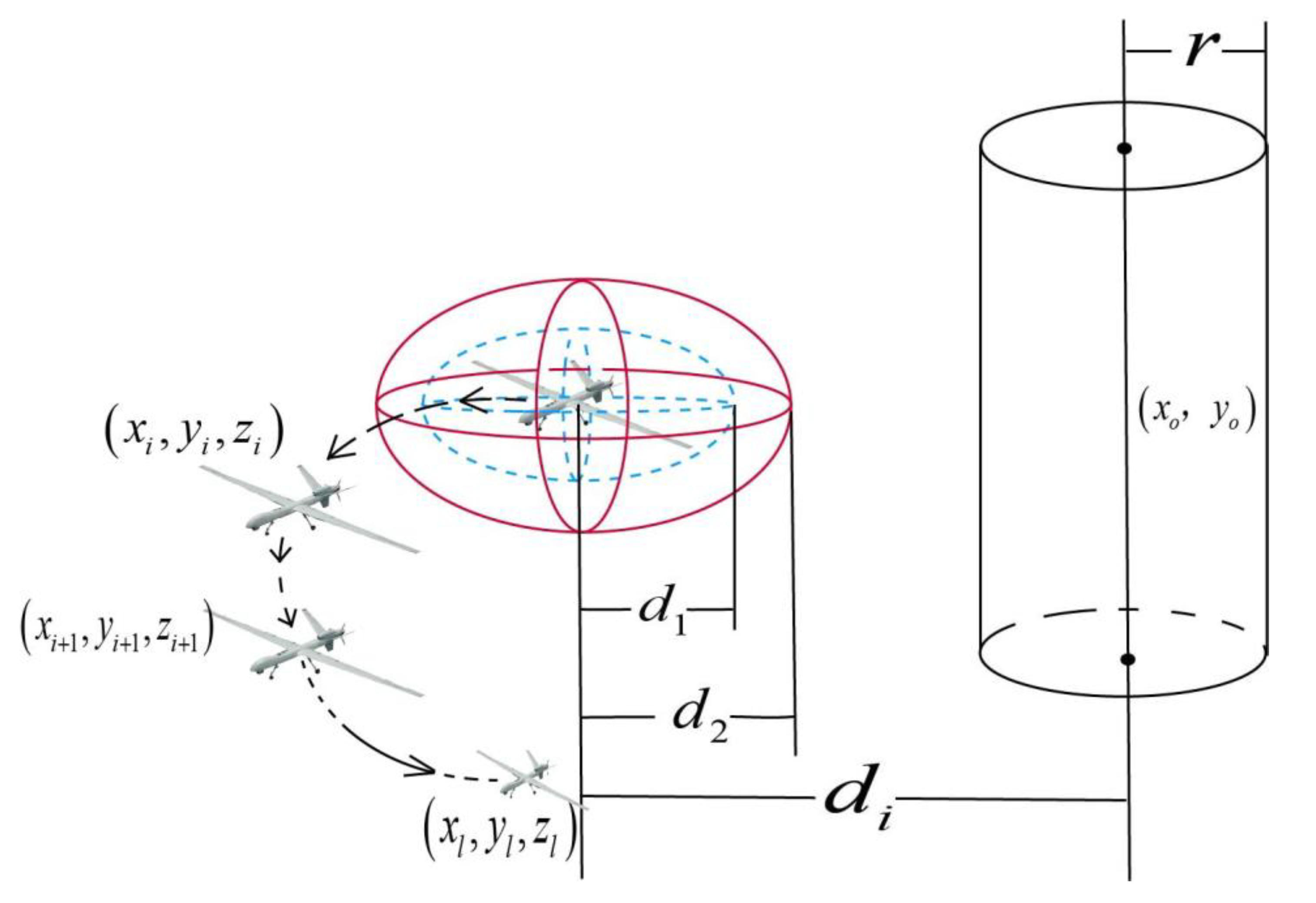
Figure 2.
Schematic of the spacing between the two drones.
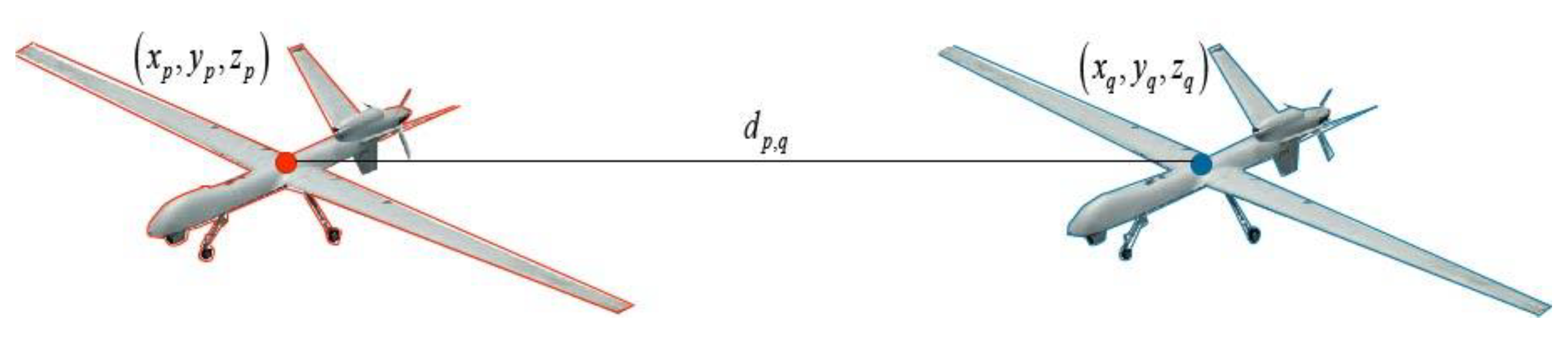
Figure 3.
Overall structure of the proposed dual-layer IALNS-IWOA framework for multi-UAV trajectory planning.
Figure 3.
Overall structure of the proposed dual-layer IALNS-IWOA framework for multi-UAV trajectory planning.
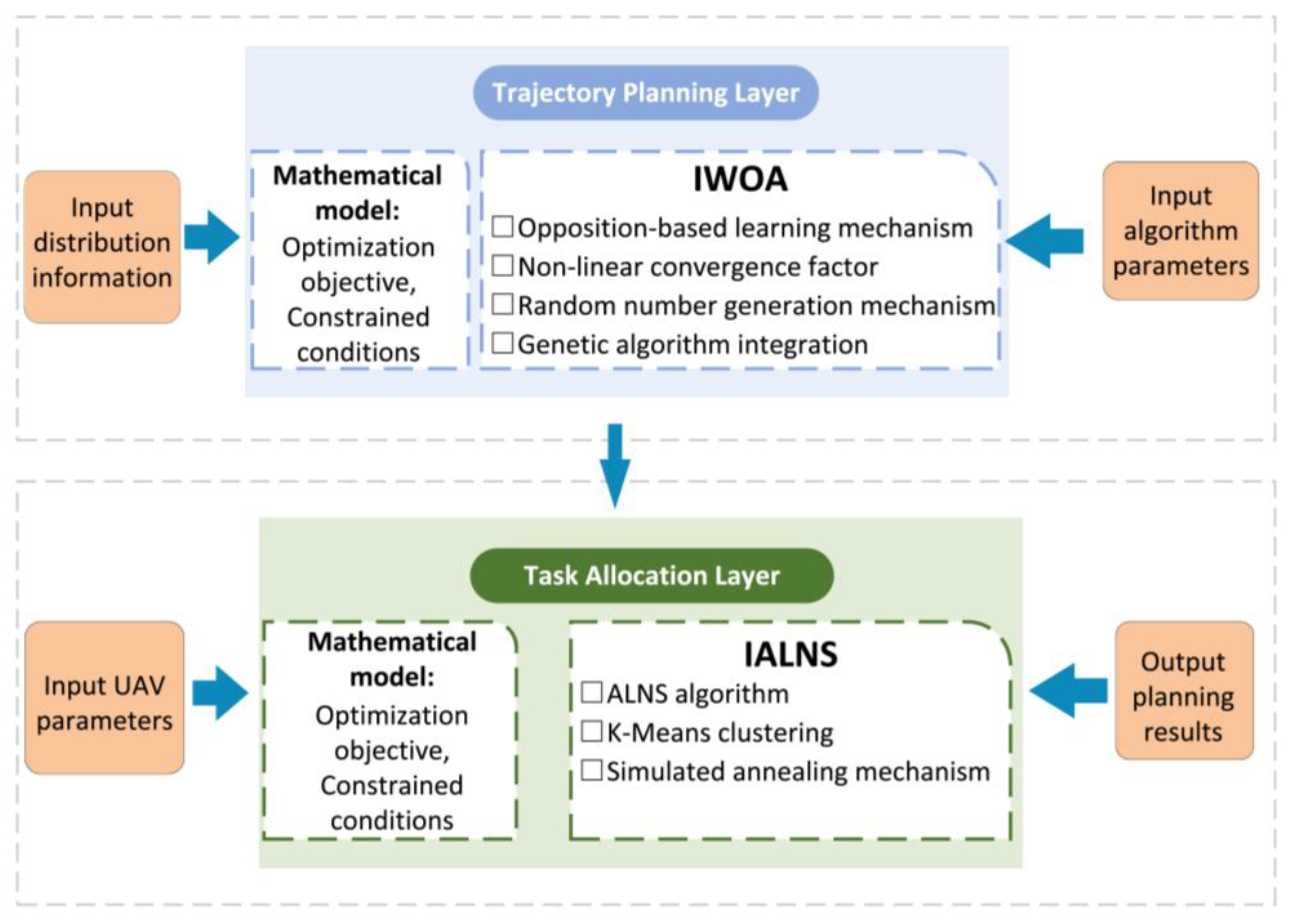
Figure 4.
Flow Chart of IALNS.
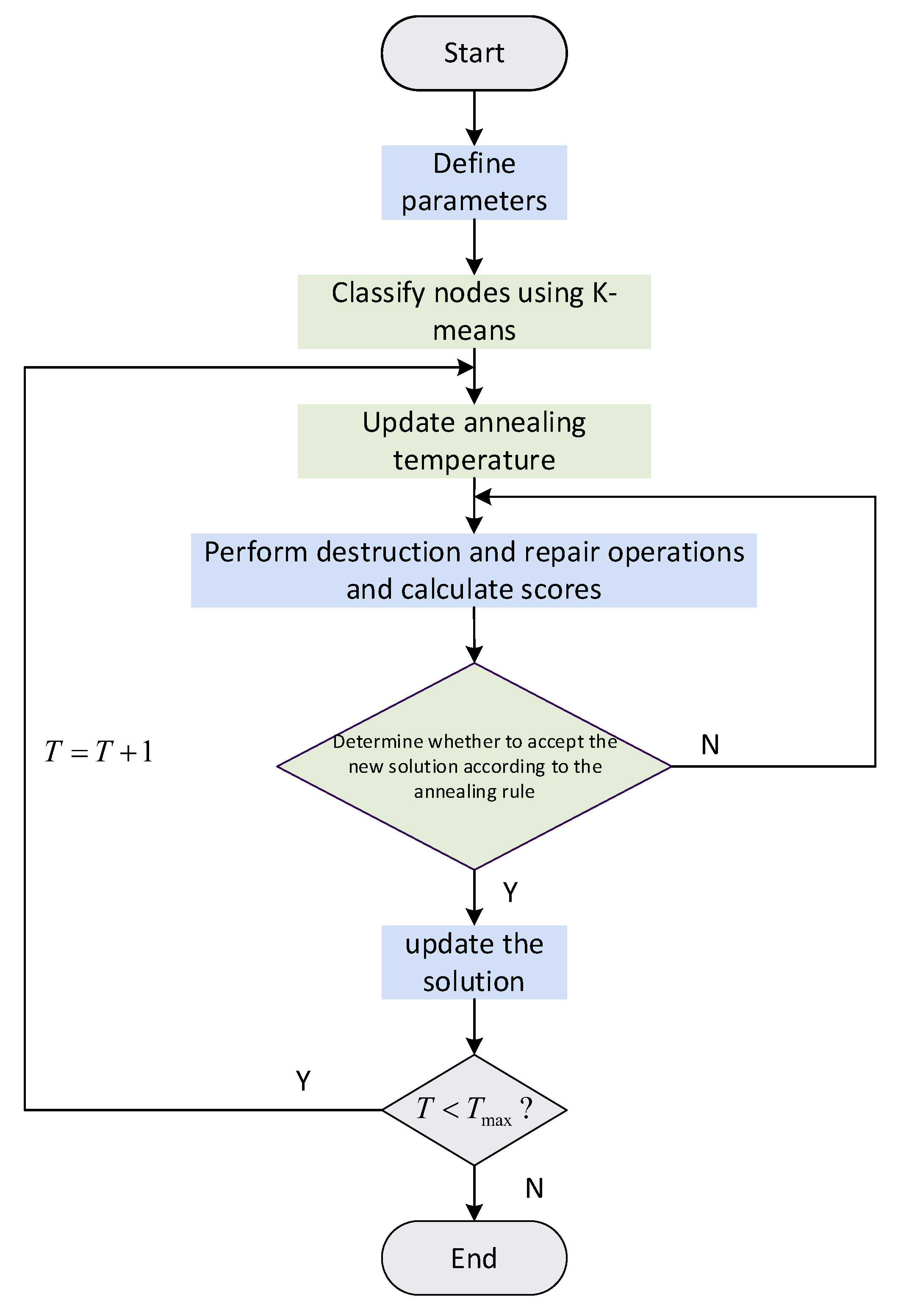
Figure 5.
K-means Clustering Diagram.
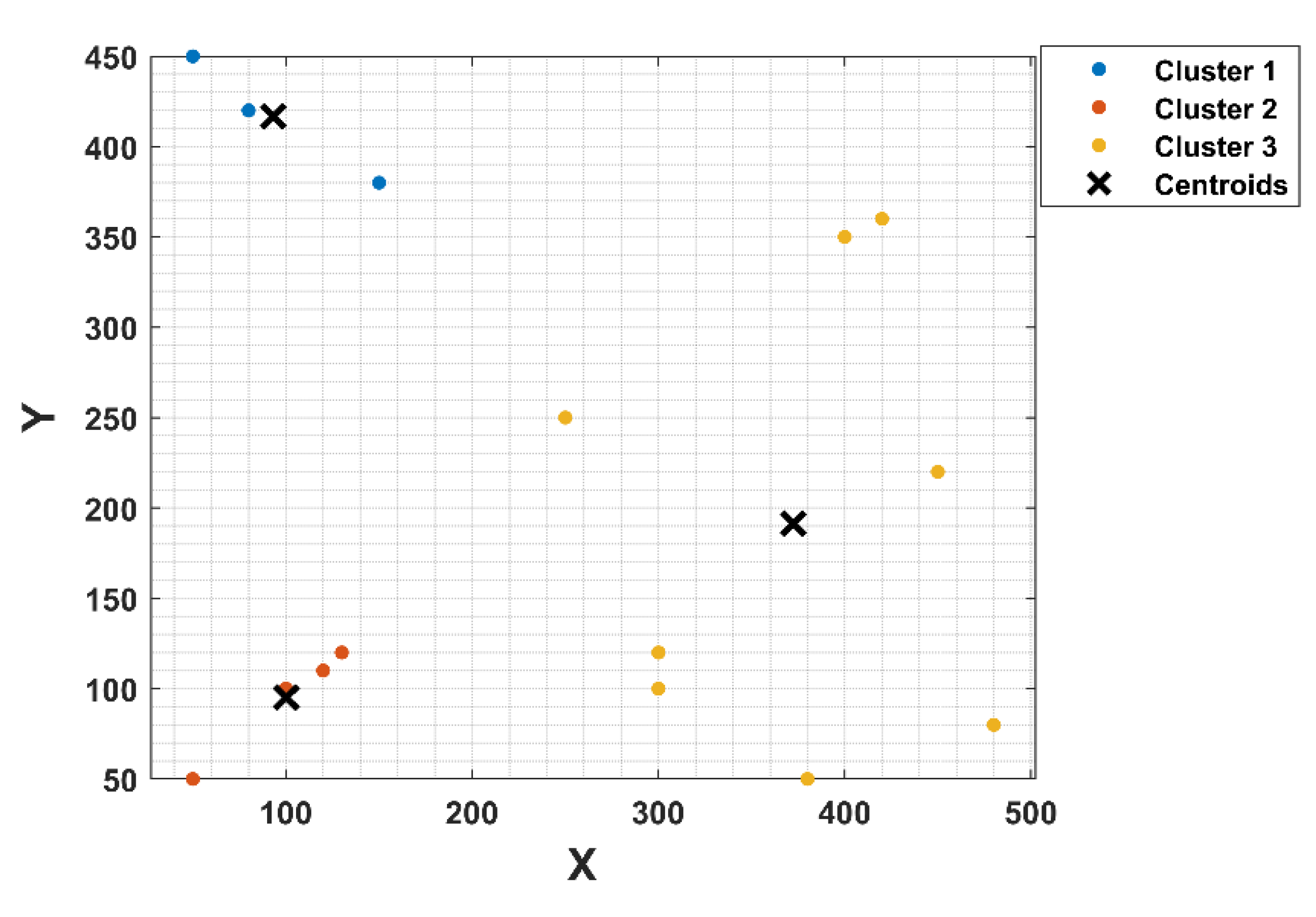
Figure 6.
IWOA Flow chart.
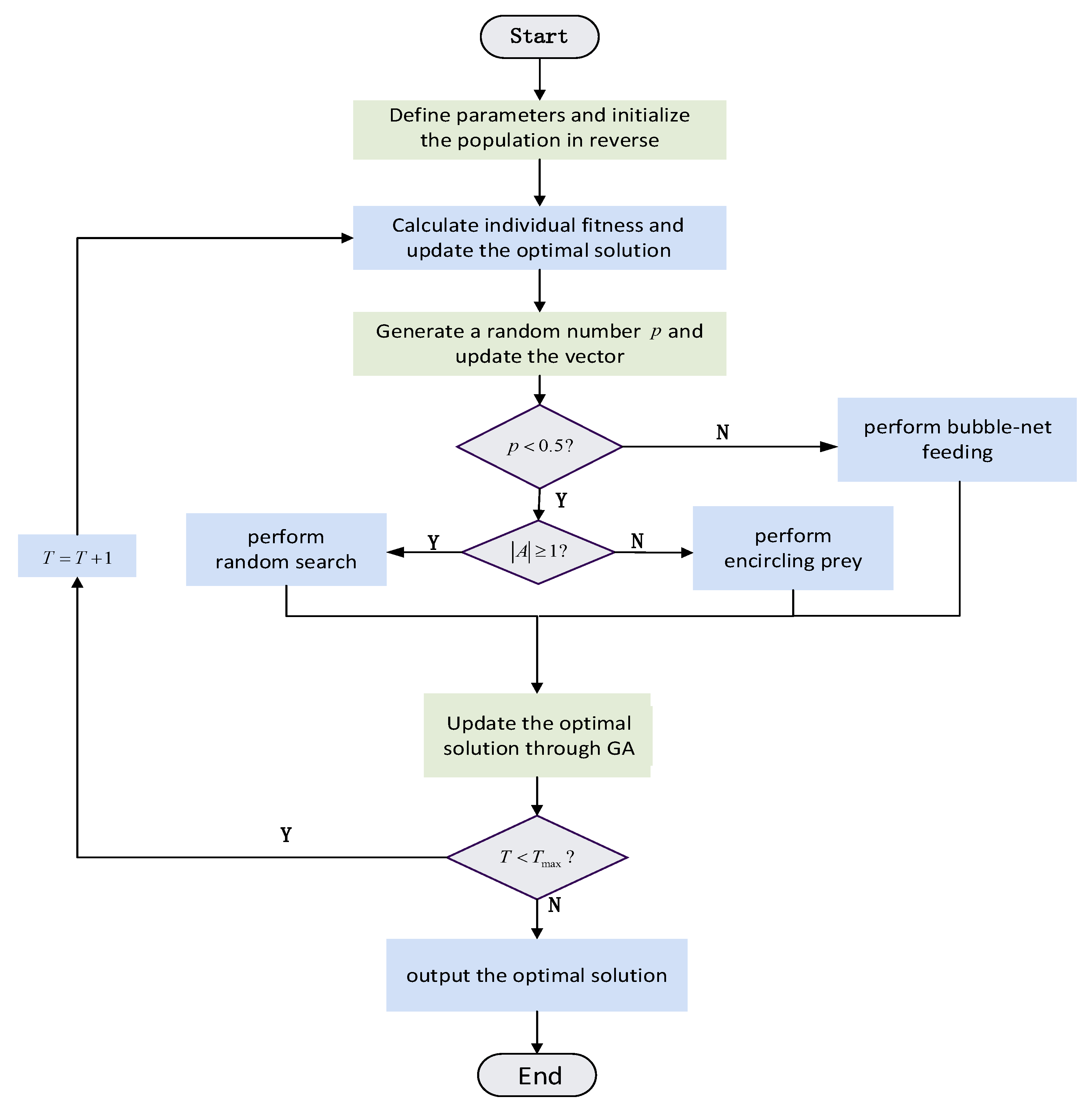
Figure 7.
Schematic Diagram of the Terrain Environment.
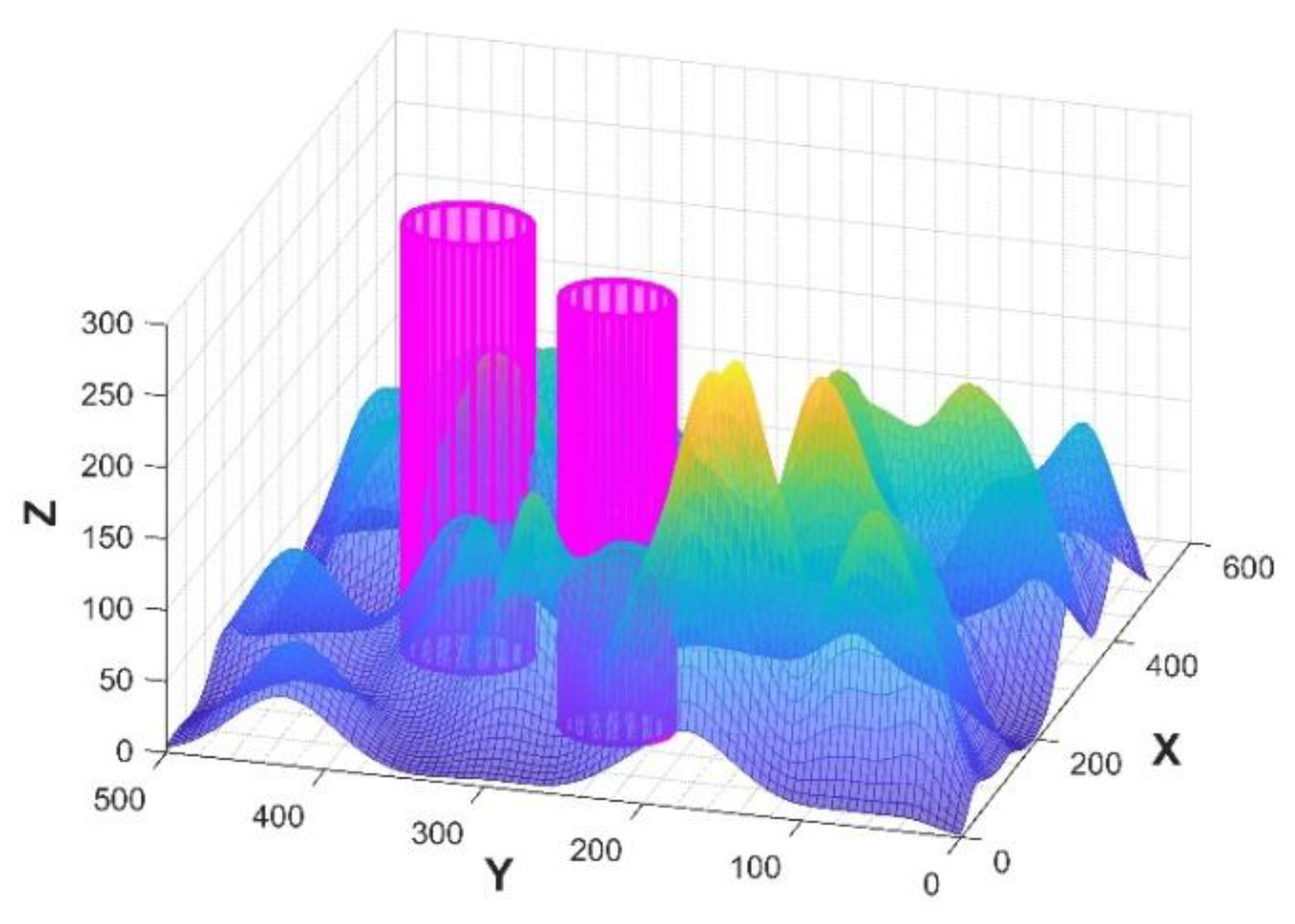
Figure 8.
Spatial distribution of mission points and depot locations over 3D terrain. (a) Side view of the terrain surface showing altitude changes and UAV start points. (b) Top view showing the 2D distribution of the 15 mission points on the terrain heat map. 02Black icons indicate depots and blue circles indicate numerically labelled mission points.
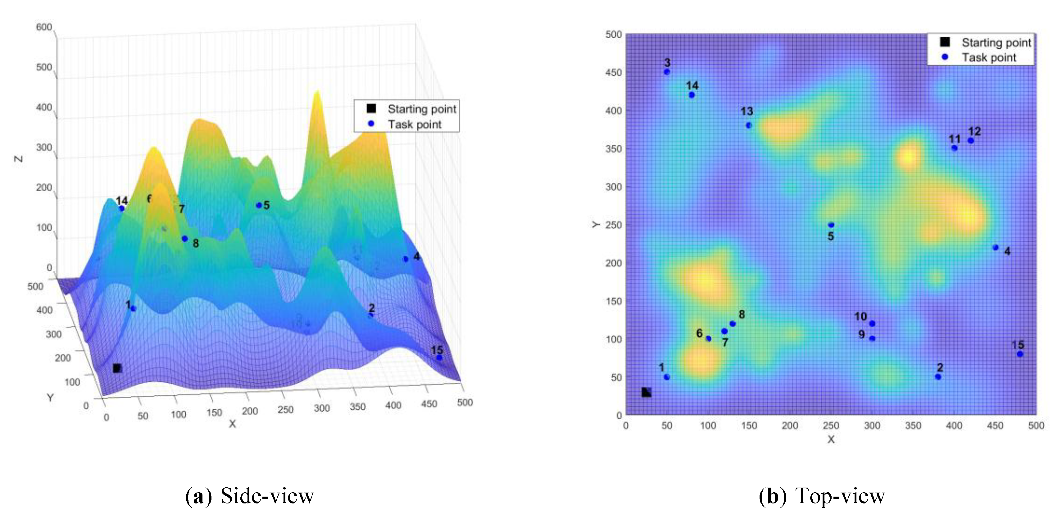
Figure 9.
Trajectory planning for the MDRP-TW problem under the IALNS-ACO algorithm.
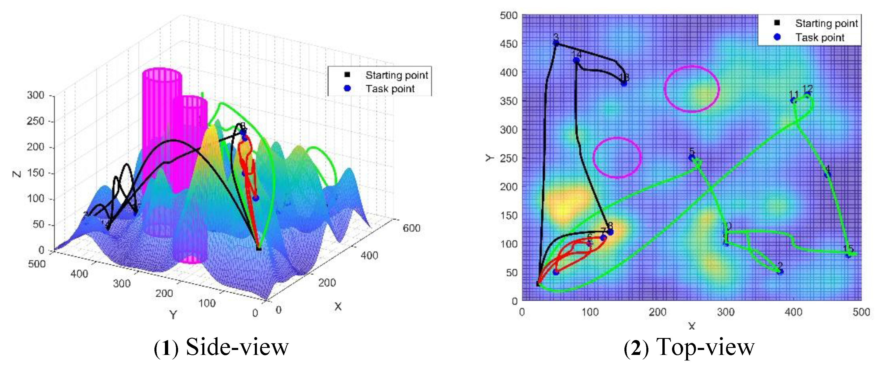
Figure 10.
Flight Path Planning Diagram. Trajectory planning for the MDRP-TW problem under the IALNS-PSO algorithm.
Figure 10.
Flight Path Planning Diagram. Trajectory planning for the MDRP-TW problem under the IALNS-PSO algorithm.
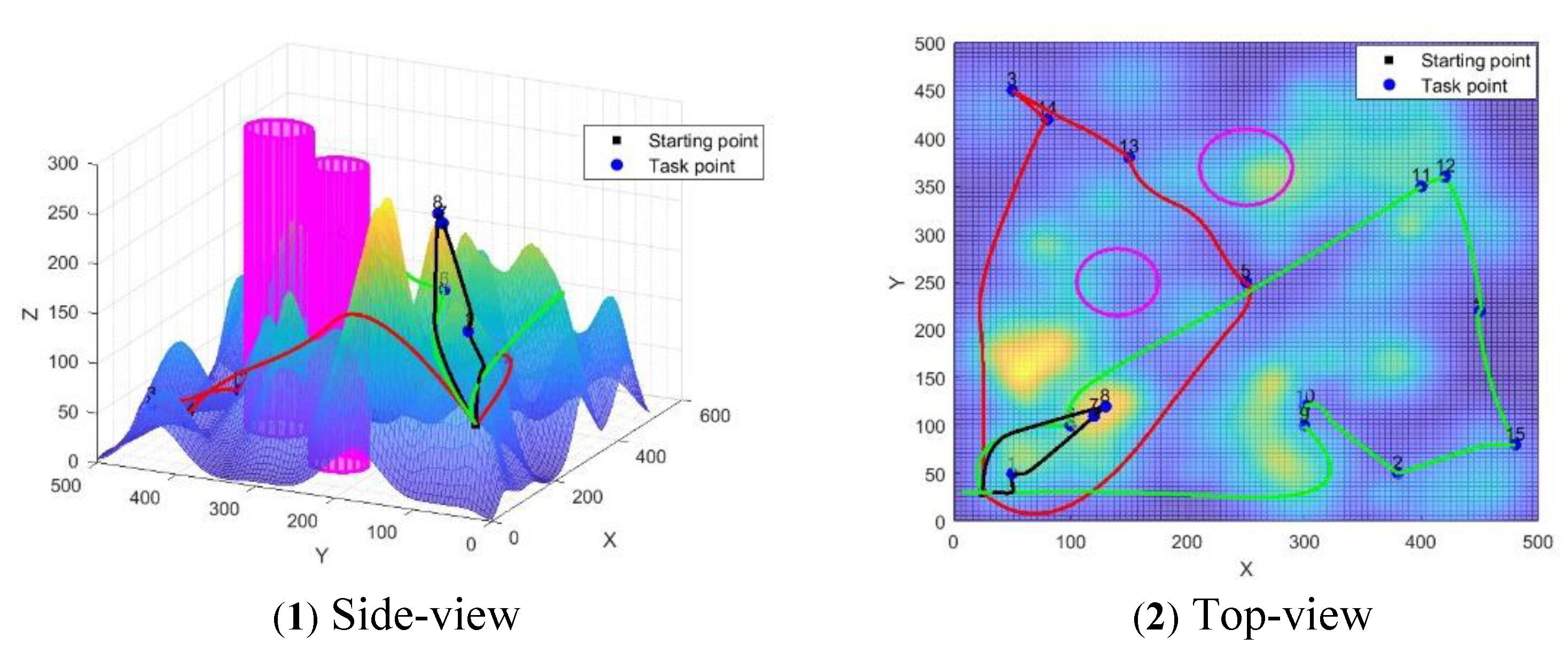
Figure 11.
Flight Path Planning Diagram. Trajectory planning for the MDRP-TW problem under the IALNS-WOA algorithm.
Figure 11.
Flight Path Planning Diagram. Trajectory planning for the MDRP-TW problem under the IALNS-WOA algorithm.
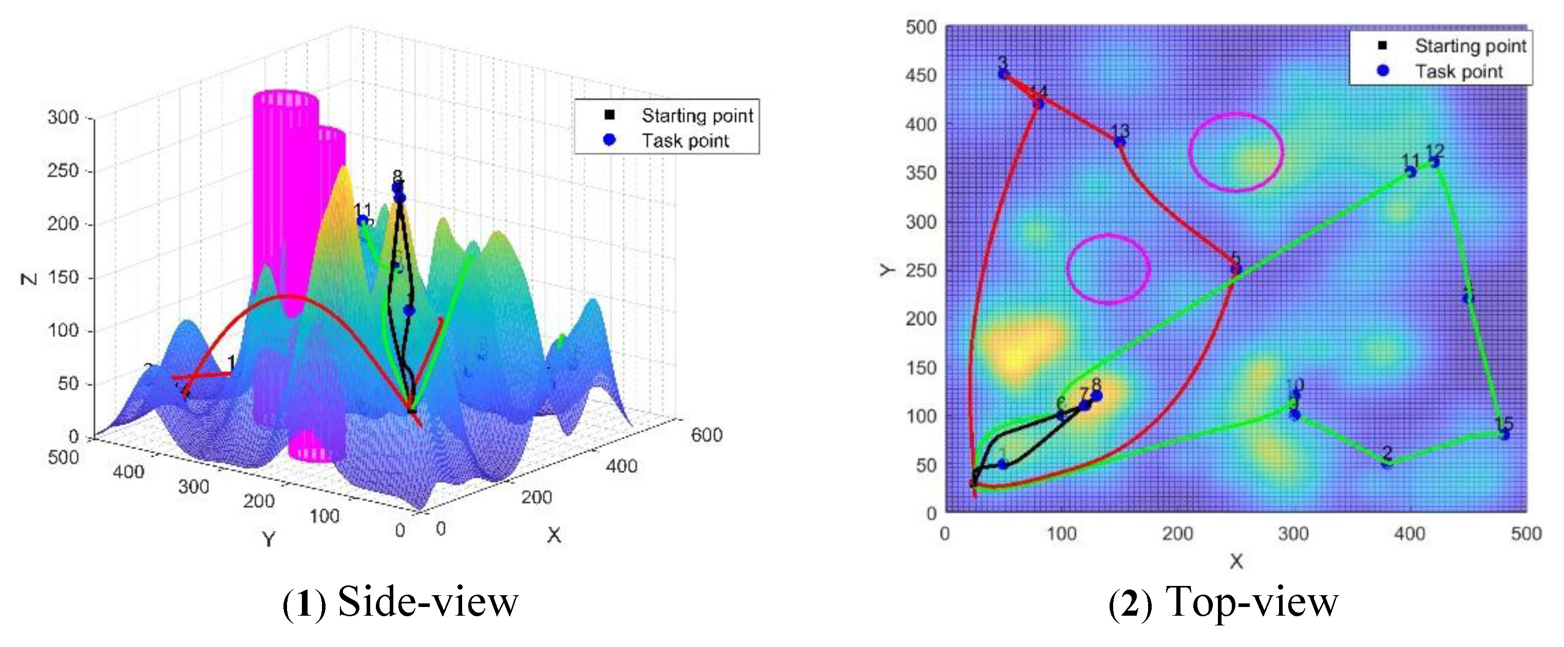
Figure 12.
Flight Path Planning Diagram. Trajectory planning for the MDRP-TW problem under the IALNS-IWOA algorithm.
Figure 12.
Flight Path Planning Diagram. Trajectory planning for the MDRP-TW problem under the IALNS-IWOA algorithm.
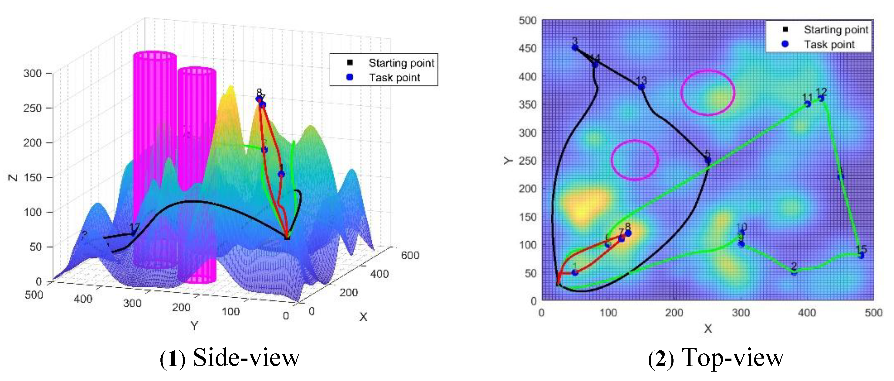
Figure 13.
Convergence comparison of different dual-layer algorithms (IALNS-IWOA, IALNS-WOA, IALNS-PSO, IALNS-ACO) over 300 iterations, evaluated by total fitness.
Figure 13.
Convergence comparison of different dual-layer algorithms (IALNS-IWOA, IALNS-WOA, IALNS-PSO, IALNS-ACO) over 300 iterations, evaluated by total fitness.
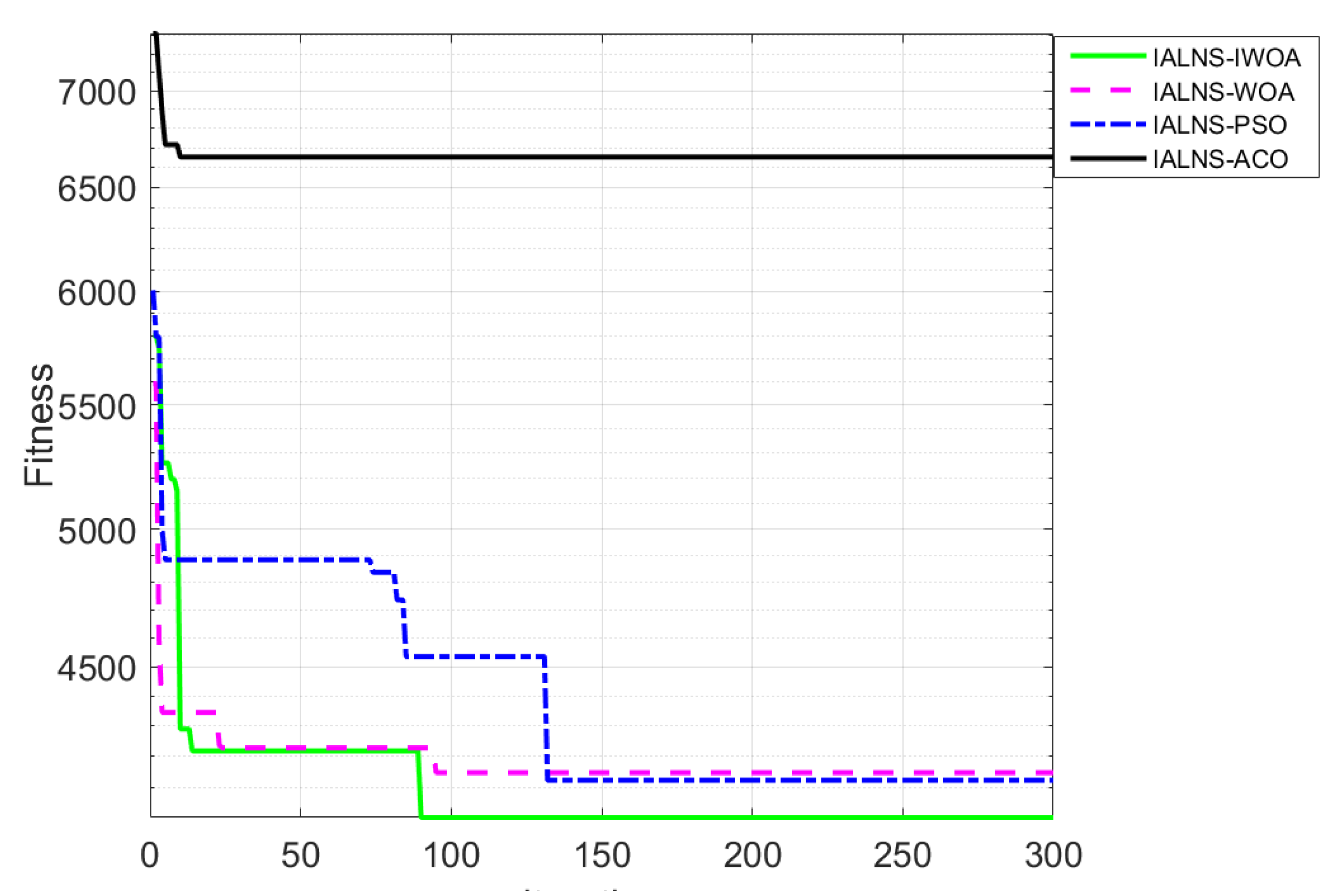
Figure 14.
Lightweight experimental simulation environment diagram.
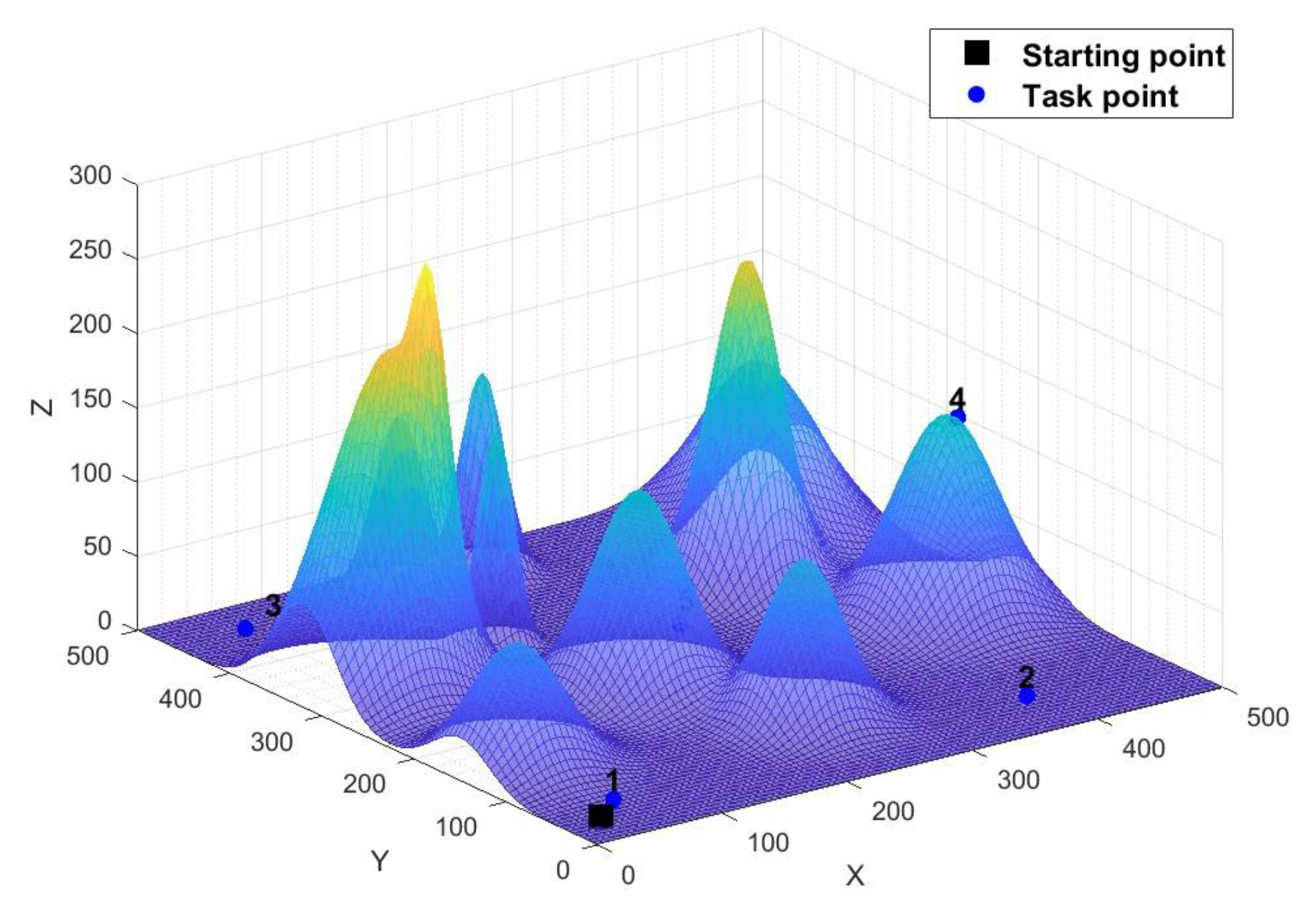
Figure 15.
Lightweight experimental drone trajectory planner.
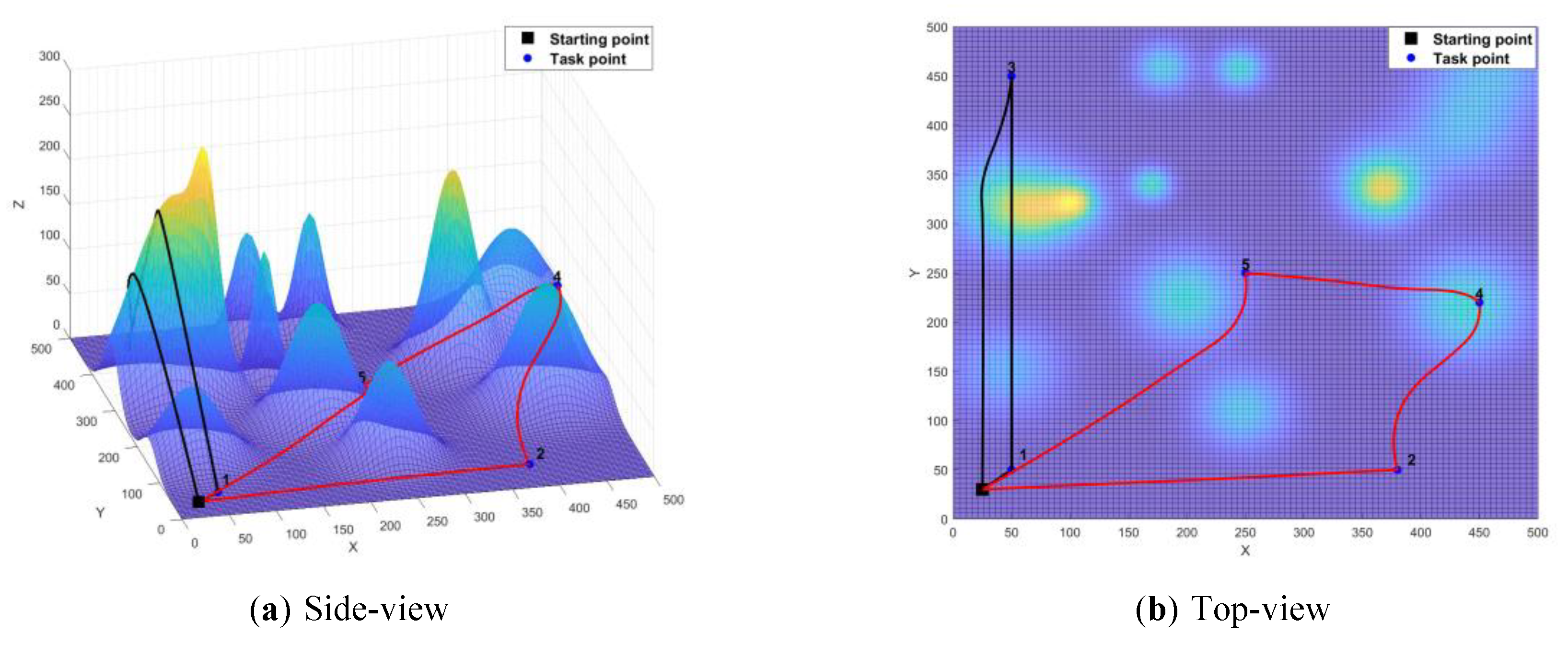
Figure 16.
Complexity experimental simulation environment diagram.
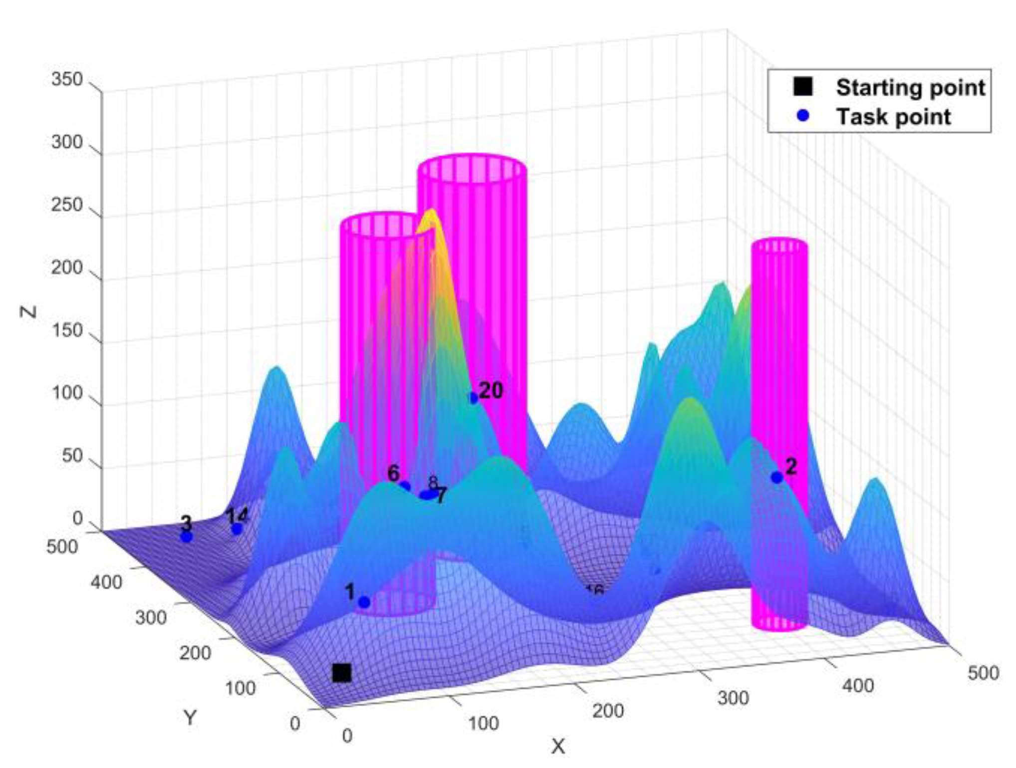
Figure 17.
Complexity experimental drone trajectory planner.
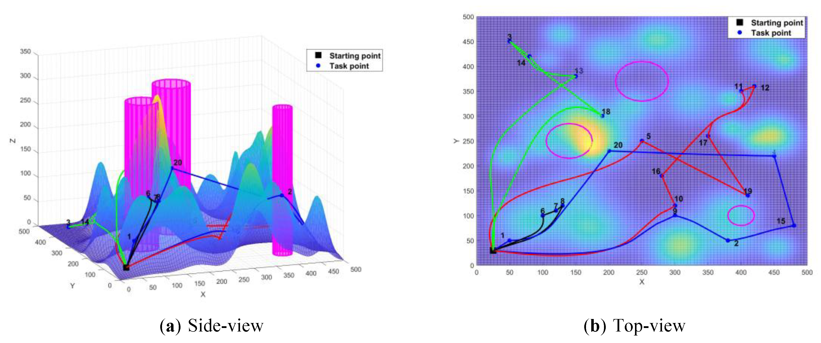

Table 1.
Description of variables and parameters used in the MDRP-TW optimization model.
| Symbol | Explanation |
|---|---|
| Euclidean distance between the and waypoints of the UAV | |
| Constraint from the waypoint to the no-fly zone | |
| Flight altitude of the UAV at the waypoint | |
| Maximum and minimum flight altitudes of the UAV | |
| Turning angle | |
| Pitch angle | |
| Distance between the and UAVs | |
| Time when the UAV arrives at the task point | |
| Left and right time windows of the task point | |
| Task volume of the task point | |
| Maximum task volume that the UAV can complete |
Table 2.
Pseudocode of the Improved Adaptive Large Neighborhood Search (IALNS) for upper-layer task assignment.
Table 2.
Pseudocode of the Improved Adaptive Large Neighborhood Search (IALNS) for upper-layer task assignment.
| Algorithm: Adaptive Large Neighborhood Search (IALNS) |
|---|
| 01: Input Clustering parameters; feasible initial solution from K-means clustering |
| 02: ; ; ; 03: Repeat 04: Update annealing temperature; update and ; select , ; 05: ; 06: Use the simulated annealing rule to determine whether to accept the new solution 07: If accepted, set ; 08: End if 09: Determine whether the new solution is accepted as the current best solution 10: If accepted, update and ; 11: End if 12: Until stopping criterion is met 13: Return the best solution |
Table 3.
Pseudocode of the Improved Whale Optimization Algorithm (IWOA) for UAV trajectory planning.
Table 3.
Pseudocode of the Improved Whale Optimization Algorithm (IWOA) for UAV trajectory planning.
| Algorithm: Improved Whale Optimization Algorithm (IWOA) |
| 01: Input Population size, maximum number of generations, search probability, variable range |
| 02: Execute reverse learning initialization to enhance population diversity 03: Evaluate the fitness value of each individual and determine the current best solution 04: Repeat 05 Calculate the nonlinear convergence factor and spiral coefficient 06 Generate a random number 07 If 08 If 09 Perform random search 10 Else: 11 Perform encircling prey 12 Else: 13 Update position using GA-based strategy 14 Update solution 15 End if 16 Determine whether termination condition is met 17 Return the best solution found |
Table 4.
Data Information Table of the No - Fly Zone.
| Serial Number | Center of the Bottom Circle | Radius |
|---|---|---|
| 1 | (250,370) | 40 |
| 2 | (140,250) | 35 |
Table 5.
Detailed attributes of task points including coordinates, demands, and time windows.
| Serial Number | X-coordinate | Y-coordinate | Demand | Left Time Window | Right Time Window | Service Time |
|---|---|---|---|---|---|---|
| Distribution Center | 25 | 30 | / | 0 | 1260 | / |
| 1 | 50 | 50 | 40 | 480 | 945 | 20 |
| 2 | 380 | 50 | 10 | 456 | 900 | 20 |
| 3 | 50 | 450 | 40 | 48 | 225 | 20 |
| 4 | 450 | 220 | 10 | 432 | 855 | 20 |
| 5 | 250 | 250 | 20 | 16 | 90 | 20 |
| 6 | 100 | 100 | 10 | 384 | 780 | 20 |
| 7 | 120 | 110 | 40 | 128 | 300 | 20 |
| 8 | 130 | 120 | 30 | 176 | 405 | 20 |
| 9 | 300 | 100 | 10 | 368 | 750 | 20 |
| 10 | 300 | 120 | 5 | 240 | 495 | 20 |
| 11 | 400 | 350 | 17 | 312 | 660 | 20 |
| 12 | 420 | 360 | 3 | 392 | 825 | 20 |
| 13 | 150 | 380 | 16 | 72 | 225 | 20 |
| 14 | 80 | 420 | 23 | 344 | 753 | 20 |
| 15 | 480 | 80 | 31 | 272 | 600 | 20 |
Table 6.
Test Functions.
| Category | Function Name | Expression | Theoretical Optimal Value |
|---|---|---|---|
| Unimodal Test Function | Sphere function | 0 | |
| Quartic Function | 0 | ||
| Multimodal Test Function | Ackley’s Function | 0 | |
| Fixed-dimension Multimodal Test Function | Branin Function | 0.39788735 | |
| Kowalik Function | 0.0003075 |
Table 7.
Performance comparison of IWOA, PSO, ACO, and standard WOA on benchmark test functions.
| Test Function | Data Type | ACO | PSO | WOA | IWOA |
|---|---|---|---|---|---|
| Mean Value | 100222.22 | 12324.9345 | 0.6090 | 0.00077 | |
| Best Value | 100222.22 | 3874.1177 | 0.05230 | 1.64983E-05 | |
| Mean Value | 5605894559 | 202601216.1 | 33.5324 | 0.119037 | |
| Best Value | 4579640494 | 37290487.49 | 1.2149 | 0.01651 | |
| Mean Value | 21.7181 | 19.9999 | 20.4272 | 20.27560 | |
| Best Value | 21.7180 | 19.9999 | 20.1486 | 20.05561 | |
| Mean Value | 15.9554 | 1.1616 | 0.6112 | 0.655569 | |
| Best Value | 14.5972 | 0.3986 | 0.3979 | 0.3979 | |
| Mean Value | 0.1170 | 0.0063 | 0.0024 | 0.0013 | |
| Best Value | 0.0156 | 0.0011 | 0.0010 | 0.0009 |
Table 8.
Optimal task allocation, flight distance, and total fitness values for different dual-layer algorithms in UAV path planning. This table summarizes the optimal results obtained from four dual-layer algorithms: IALNS-IWOA, IALNS-WOA, IALNS-PSO, and IALNS-ACO. For each algorithm, the task sequences, flight distances, task volumes, total distances, and overall fitness values are presented across three UAVs.
| Algorithm | Drone | Task Points | Flight Distance | Task Volume | Total Flight Distance | Total Fitness |
|---|---|---|---|---|---|---|
| IALNS-IWOA | 1 | 0-8-7-1-0 | 461.30792 | 110 | 2961.5315 | 4019.38625 |
| 2 | 0-5-13-3-14-0 | 1054.25558 | 99 | |||
| 3 | 0-10-9-2-15-4-12-11-6-0 | 1445.96800 | 96 | |||
| IALNS-WOA | 1 | 0-13-3-14-10-9-0 | 1227.17871 | 94 | 3194.65192 | 4338.738 |
| 2 | 0-7-8-1-0 | 462.48449 | 110 | |||
| 3 | 0-5-11-12-4-15-2-6-0 | 1504.98872 | 101 | |||
| IALNS-PSO | 1 | 0-7-8-1-0 | 462.48449 | 110 | 3063.74593 | 4147.02121 |
| 2 | 0-5-13-3-14-0 | 1054.25558 | 99 | |||
| 3 | 0-9-10-2-15-4-12-11-6-0 | 1547.00586 | 96 | |||
| IALNS-ACO | 1 | 0-7-1-6-0 | 566.87832 | 90 | 3543.66885 | 6603.29729 |
| 2 | 0-3-13-14-8-0 | 1238.45150 | 109 | |||
| 3 | 0-5-10-2-9-15-4-12-11-0 | 1738.33903 | 106 |
Table 9.
Lightweight Experimental UAV Flight Path Planning Trajectory Information Sheet.
| Algorithm | Drone | Task Points | Flight Distance | Task Volume | Total Flight Distance | Total Fitness |
|---|---|---|---|---|---|---|
| IALNS-IWOA | 1 | 0-3-1-0 | 852.76203 | 80 | 1973.14747 | 998.83682 |
| 2 | 0-5-4-2-0 | 1120.38544 | 40 |
Table 10.
Additional task point information sheet.
| Serial Number | X-coordinate | Y-coordinate | Demand | Left Time Window | Right Time Window | Service Time |
|---|---|---|---|---|---|---|
| 16 | 280 | 180 | 12 | 256 | 540 | 20 |
| 17 | 350 | 260 | 25 | 144 | 330 | 20 |
| 18 | 190 | 300 | 28 | 320 | 660 | 20 |
| 19 | 410 | 140 | 14 | 192 | 420 | 20 |
| 20 | 200 | 230 | 9 | 400 | 810 | 20 |
Table 11.
Added no-fly zone data information sheet.
| Center of the Bottom Circle | Radius |
|---|---|
| (400,100) | 20 |
Table 12.
Lightweight Experimental UAV Flight Path Planning Trajectory Information Sheet.
| Algorithm | Drone | Task Points | Flight Distance | Task Volume | Total Flight Distance | Total Fitness |
|---|---|---|---|---|---|---|
| IALNS-IWOA | 1 | 0-8-7-6-0 | 372.88136 | 80 | 4130.72609 | 1953.13468 |
| 2 | 0-5-19-17-11-12-16-10-0 | 1366.03646 | 96 | |||
| 3 | 0-13-3-14-18-0 | 1085.99370 | 107 | |||
| 4 | 0-9-2-15-4-20-1-0 | 1305.81457 | 110 |
Disclaimer/Publisher’s Note: The statements, opinions and data contained in all publications are solely those of the individual author(s) and contributor(s) and not of MDPI and/or the editor(s). MDPI and/or the editor(s) disclaim responsibility for any injury to people or property resulting from any ideas, methods, instructions or products referred to in the content. |
© 2025 by the authors. Licensee MDPI, Basel, Switzerland. This article is an open access article distributed under the terms and conditions of the Creative Commons Attribution (CC BY) license (http://creativecommons.org/licenses/by/4.0/).
Copyright: This open access article is published under a Creative Commons CC BY 4.0 license, which permit the free download, distribution, and reuse, provided that the author and preprint are cited in any reuse.


