
Submitted:
17 June 2024
Posted:
17 June 2024
You are already at the latest version
Abstract
The challenging terrain and deep ravines characteristic of mountainous regions often result in slower path planning and suboptimal flight paths for Unmanned Aerial Vehicles (UAVs) when traditional meta-heuristic optimization algorithms are employed. This study investigates the application of an Improved Enhanced Snake Optimizer (IESO) for three-dimensional path planning in a simulated rugged mountainous terrain. The initialization process in the enhanced snake optimizer is refined by integrating the Chebyshev chaotic map. Additionally, a non-monotonic factor is introduced to modulate the "temperature," and a boundary condition is incorporated into the dynamic opposition learning mechanism. These modifications collectively reduce the likelihood of population convergence to local optima during optimization. The feasibility of IESO is validated through time complexity and global convergence analyses. Comparative simulation experiments benchmarked IESO against five state-of-the-art optimization algorithms across test functions and path-planning simulated scenarios. The experimental results indicate that the enhanced algorithm achieves superior optimization precision, faster convergence speeds, and improved quality in the planned trajectories by 30%.
Keywords:
UAV
; path planning
; enhanced snake optimizer
; dynamic boundary-based opposition learning
; test function
1. Introduction
The complex mountainous terrain, characterized by significant elevation changes and limited transportation options, often renders certain areas difficult to access using conventional observation, surveillance, and logistical support methods. Due to their agility and flexibility, unmanned aerial vehicles (UAVs) have become extensively utilized in these challenging environments. Consequently, high-quality and rapid flight path planning in such complex terrains is critically important for enhancing the efficiency of UAV missions [1,2].
Recent research in UAV path planning has introduced many different methodologies, including meta-heuristic optimization algorithms (MAs) [3], the quality-oriented hybrid A* and Q-learning algorithm [4], the artificial potential field [5], trajectory planning with matrix alignment Dijkstra’s algorithm [6,7]. Flores-Caballero et al. [8] approached path planning as a constrained global optimization problem, utilizing MAs in conjunction with the A* algorithm. However, their objective function was overly simplistic, concentrating exclusively on flight distance, and consequently, it did not achieve optimal practical outcomes. Shao et al. [9] proposed a hierarchical trajectory optimization framework that combines an adaptive particle swarm optimization algorithm with the Gaussian pseudospectral method. This methodology accounted for the UAV dynamics model and state constraints, thereby enabling the minimization of flight time. However, the simulated environment was overly simplistic and not applicable to complex terrains, such as mountainous regions or ravines. For large-scale collaborative searches, Chen et al. [10] utilized the ant colony optimization algorithm to efficiently plan paths for UAV swarms, reducing task completion times. Despite its rapid optimization, the algorithm exhibited limited convergence precision.
UAV path planning necessitates considering rugged terrain environments, such as mountainous regions, flight safety, and UAV-specific conditions, rendering it a quintessential multi-objective optimization problem. A literature review reveals that current research predominantly focuses on MAs due to their global search capabilities, which effectively address UAV motion constraints and path planning requirements, particularly in complex environments characterized by rugged mountainous terrain.
In this study, we examined the Enhanced Snake Optimizer (ESO) proposed by Yao et al. [11], which builds upon the original Snake Optimizer (SO) developed by Hashim and Hussien [12]. The ESO incorporates a randomized population initialization and mirroring imaging. This enhancement has been validated using classical test and engineering design functions, demonstrating its applicability to UAV path planning. However, in line with the No Free Lunch theorem [13], which posits that no single algorithm is universally optimal for all optimization problems, we acknowledge the limitations of ESO.
We propose three major ESO revisions at three stages that significantly improve optimization results, particularly in rugged terrains. Therefore, we name our method Improved Enhanced Snake Optimizer (IESO). First, the original SO employs a simple normal distribution random function to initialize the "population," which consists of the initial guess points. We replaced this with a Chebyshev chaotic map to improve the diversity and quality of the initial population. Second, we introduced a non-monotonic coefficient to adjust the "temperature," which controls the search merge and split processes. This modification addresses the SO’s persistent "cold temperature" state, balancing global exploration and local exploitation. Third, we added a boundary value to address occasional anomalies from the dynamic opposition learning mechanism, a key enhancement of ESO over SO.
With these three major revisions to ESO, we tested IESO against five state-of-the-art optimization algorithms, namely Enhanced Snake Optimizer (ESO) [11], Snake Optimizer (SO) [12], Golden Jackal Optimization (GJO) [14], Honey Badger Algorithm (HBA) [15], Grey Wolf Optimizer (GWO) [16], demonstrating superior performance in precision, convergence speed and planned trajectory quality.
2. Methodologies: Improved Enhanced Snake Optimizer (IESO) Algorithm and Simulation Design
This section is organized into four subsections: 2.1 briefly reviews the Snake Optimizer (SO). 2.2 presents a concise overview of the Enhanced Snake Optimizer (ESO). 2.3 offers a detailed explanation of our Improved Enhanced Snake Optimizer (IESO). 2.4 discusses the design of the simulation experiments and the evaluation criteria.
2.1. Basic Concepts of Snake Optimizer (SO)
The Snake Optimizer (SO) was initially proposed by Hashim and Hussien [12] in 2022. It is an optimization algorithm inspired by the snake mating process, which is influenced by "temperature" (mode switch) and "food" (change position) availability. Snakes mate only when the temperature is low, and food is abundant. When food is scarce, the SO algorithm prioritizes the food search, representing the exploration phase (global search). Once food is sufficient, the algorithm progresses to the exploitation phase (local search). During "hot" temperatures (T > 0.6), mating is deferred. When temperatures are low (T < 0.6), snakes engage in mating, based on a random probability (0, 1), whether to mate with the opposite sex or engage in same-sex aggression. When , mating behaviour occurs between sexes; while < 0.6, males compete for mating rights in a fight mode, followed by a mating mode. Successful mating results in females laying eggs and hatching new snakes, thereby renewing the population (add more search points).
In SO, the "population" (N) represents the search points. The initial positions are generated using a random uniform distribution function, as defined in Equation 1. The population is then equally divided into two groups: males and females.
In SO, The "temperature" (T) determines the switch between global and local search modes. It is defined by Equation 2, where t is the current iteration and T is the maximum iteration and the same for the rest of this manuscript.
In SO, a "food" parameter represents the feature position. The algorithm performs a broad, global search when no food is available. If food is present and the temperature is "hot", the algorithm refines the search point positions by eating food. When the temperature is "cold," the algorithm enters the exploitation phase, where males and females select optimal mates, resulting in convergence and repositioning new search points. The food quantity (Q) is defined in Eq. 3.
When Q < 0.25, the snakes search for food by selecting any random position and updating their position for it, which is called the exploration phase. The male version is presented as Eq. 4, and is defined as Eq. 5. The female version is identical except for replacing the subscript m to f.
When Q > 0.6 and T > 0.6, the snake searches for food, keeping the global search. And it is presented in Eq. 6.
where is the snake position (male or female), is the position of the food.
When Q > 0.6 and T < 0.6, the snake will enter the flight mode (FM) or mating mode (MM), which means the search points are merging and splitting, which are presented in Eq. 7 and 8.
where is the male position, refers to the best female position. FM and FF are the fighting ability of a snake (male and female), and it is defined in Eq. 9 and 10.
2.2. Enhanced Snake Optimizer (ESO)
The Enhanced Snake Optimizer (ESO) was proposed by Yao et al. in 2023 [11]. The main modifications are the dynamic coefficients. First, the food quantity initialization function opens the fixed coefficient = 0.5 to a dynamic updated , given as Eq. 17.
where is a random number between (0,1).
Then, the fixed temperature coefficient = 0.05 to a new dynamic as shown in Eq. .
where is a random number between (0,1). And, the fixed = 2.
2.3. Improved Enhanced Snake Optimizer (IESO)
In our Improved Enhanced Snake Optimizer (IESO), we have implemented three significant enhancements based on the Enhanced Snake Optimizer (ESO). First, we adopted Chebyshev Population Initialization to initialize the snake’s initial population. Second, we introduced a non-monotonic factor to modulate the temperature. Third, we applied a Dynamic Boundary-based Opposition Learning (DBOL) approach to define the upper and lower boundaries. The general flowchart is illustrated in Figure 1.
2.3.1. Chebyshev Population Initialization
The SO and ESO randomly populate the initial population, leading to unstable target accuracy and varying convergence speeds across multiple searches. Achieving a more evenly distributed initial population within the solution space enhances the probability of locating the optimal value. Chaotic search, renowned for its randomness, ergodicity, and uniqueness, is preferred over random search strategies for generating initial populations due to its thorough coverage of the solution space. Therefore, this paper employs the Chebyshev chaotic map [19] for initializing the snake population to ensure a more comprehensive occupation of the entire solution space. The mathematical model of the Chebyshev chaotic map is as follows Eq. 21:
This comparison, illustrated in Figure 2a,b, demonstrates that the Chebyshev chaotic map produces a more uniformly distributed initial population. The Chebyshev chaotic map exhibits enhanced search capabilities, particularly when solutions to constrained problems are situated at the boundaries of the search space.
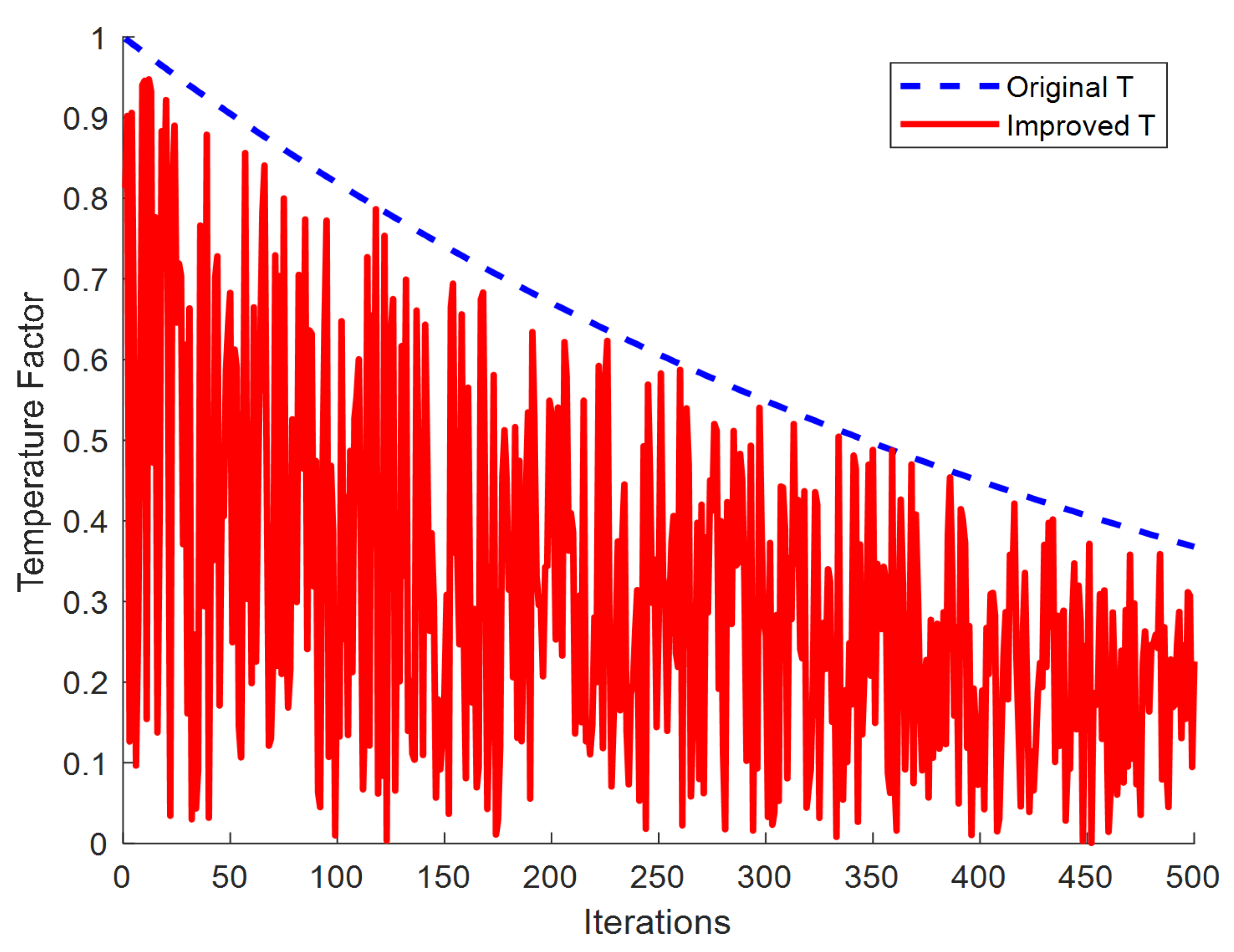
2.3.2. Non-Monotone Temperature Factor
In SO and ESO, the temperature factor influences the behaviour of the snake swarm in a monotonic manner. Figure 2 demonstrates that the temperature factor solely depends on the number of iterations, with a threshold value of approximately 220. Before this threshold, the temperature coefficient T consistently remains above 0.6, indicating a "warm" state and foraging activity. Conversely, as the optimization process progresses into its later stages, the temperature shifts to a "cold" state and remains "cold." This transition indicates that after a significant number of iterations, both SO and ESO are prone to local convergence failure.
To address this issue, we introduce a non-monotonic temperature factor by incorporating a random coefficient a into each iteration’s temperature coefficient T. This adjustment allows the modified temperature coefficient to balance more effectively between local development modes, as shown in Equation 22.
Figure 3.
Temperature factor.
2.3.3. Dynamic Boundary-Based Opposition Learning (DBOL)
After carefully examining the mirror imaging strategy used in ESO [17] and the original opposition-based learning (OBL) [18], it is evident that the ESO mirror method effectively enhances the diversity and quality of the population by calculating the opposition solutions for the current position and then selecting the optimal solution.
However, the performance exhibits a certain degree of uncertainty. While opposition solutions may have greater potential for global optimization, the fixed search upper and lower boundaries limit the ability to estimate the direction of new solutions. We propose a Dynamic Boundary-based Opposition Learning (DBOL) to address this issue. DBOL leverages the fact that elite individuals carry more effective information than ordinary ones to refine the opposition process. It fully utilizes the valuable experiences of historical individuals while maintaining a global perspective for new individuals. Through greedy selection, a superior solution is chosen between the current and opposition solutions to participate in the next iteration. The DBOL defines the boundary as follows: Eq. 23:
where is a random value in the interval (0, 1), , , and and are the upper and lower dynamic boundary in the dimension, respectively.
2.4. Simulation Experiments Design and the Evaluation Criteria
2.4.1. Simulated Experiment
This study’s simulation experiments are divided into two parts: The first part involves selecting the benchmark test functions with a search dimension (D=1000). The objective is to compare different algorithms’ convergence speeds and optimization precision to ascertain whether IESO demonstrates a superior capability to evade local optima when dealing with large-scale optimization problems. The second part entails creating a simulated rugged mountainous terrain to test the path planning. In this experience, the performance of various algorithms is assessed when solving three-dimensional path planning problems based on the three optimization criteria (discussed in 2.4.2). It aims to further validate the feasibility of IESO in determining optimal flight paths within intricate, complex landscapes.
We selected thirteen testing functions shown in Table 1.
We selected five algorithms, namely GJO, GWO, HBA, ESO and SO and their parameters are listed in Table 2.
We randomly generated the digital elevation model of a simulated rugged mountainous terrain, with map dimensions of 100 km by 150 km by 3 km. The maximum elevation difference is at least 2 km, representing a terrain with significant undulations and numerous ravines. Arbitrary no-fly zones were also added to increase the complexity. Flight waypoints were set to evaluate the effectiveness of the flight paths generated by different algorithms.
The experimental setup utilized a Windows 10, 64-bit operating system with an AMD Ryzen 7 4800H CPU running at 2.9 GHz and 16GB of RAM. The algorithms were implemented on the Matlab2020b platform.
2.4.2. Evaluation Criteria
Considering the intricate nature of UAV three-dimensional path planning, this study formulates the path planning objective function by incorporating factors such as flight distance, path smoothness, and flight safety. The shortest flight path is defined as Eq. 24
, where D represents the number of waypoints and denotes the cooridnates of the waypoints. Ensuring smoothness involves minimizing abrupt changes in yaw angle and altitude. Given mountainous areas’ rugged and diverse terrain, flight paths must adhere to maximum climb angles and rates. The path smoothness is given as Eq. 25, 26, and 27.
where represents the distance between two waypoints. Eq 25 and 26 represent the yaw angle and pitch angle , respectively.
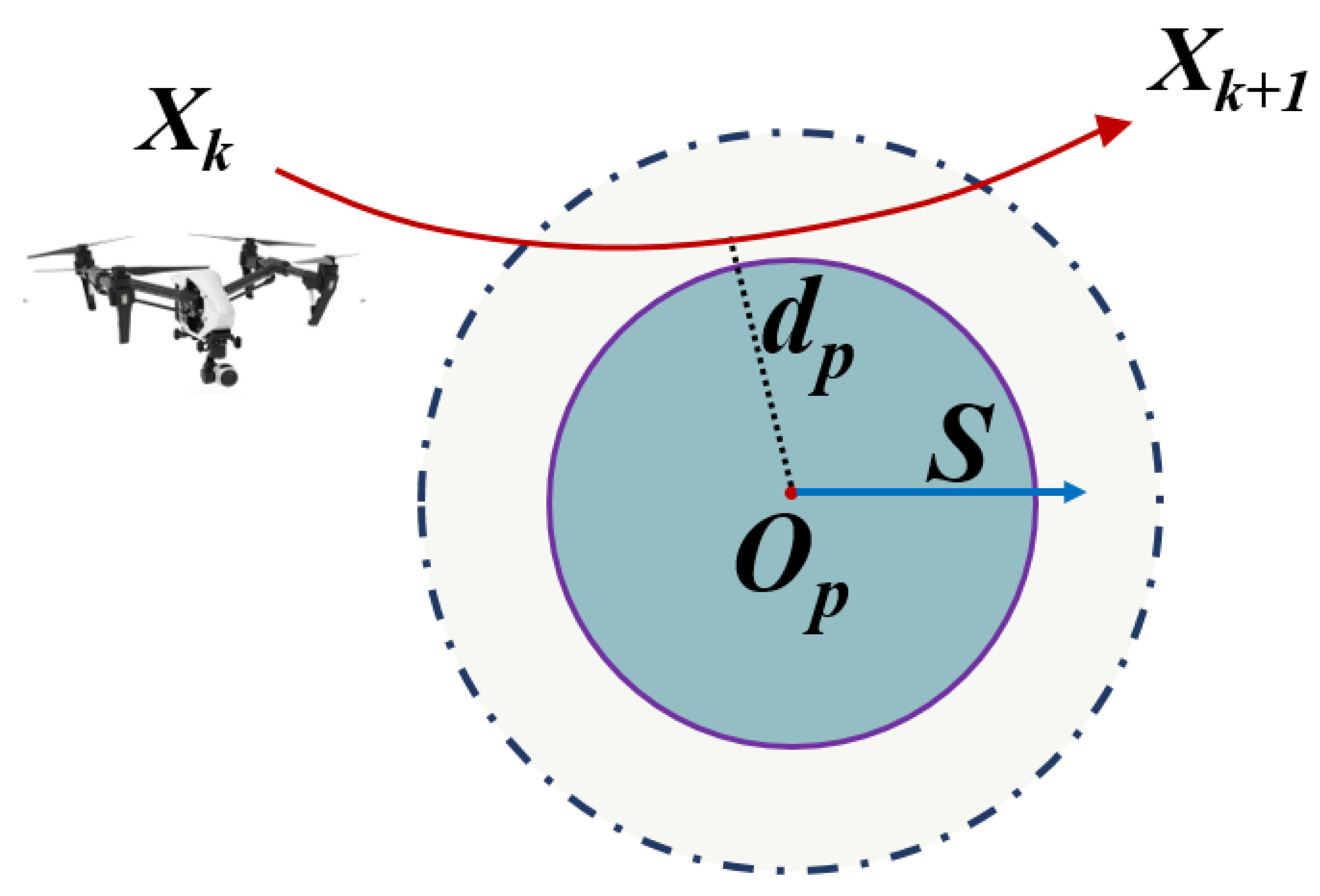
A meticulously designed path should prioritize the safe operation of UAVs. The objective function design must incorporate a safety margin, enabling UAVs to avoid obstacles or restricted no-fly zones. As shown in Figure 4 the obstacle within the airspace has a center coordinate of and radius . The perpendicular distance from the flight node of the UAV to the obstacle should exceed the safety distance , ensuring the UAV operates outside designated shaded regions for safety. The flight safety formula is provided as Eq. 28
By integrating these cost functions with weights, an objective function F for the multi-objective path planning problem is formed in Eq. 29
Figure 4.
Flight safety to avoid obstacles or restricted no-fly zones.
3. Results and Discussion
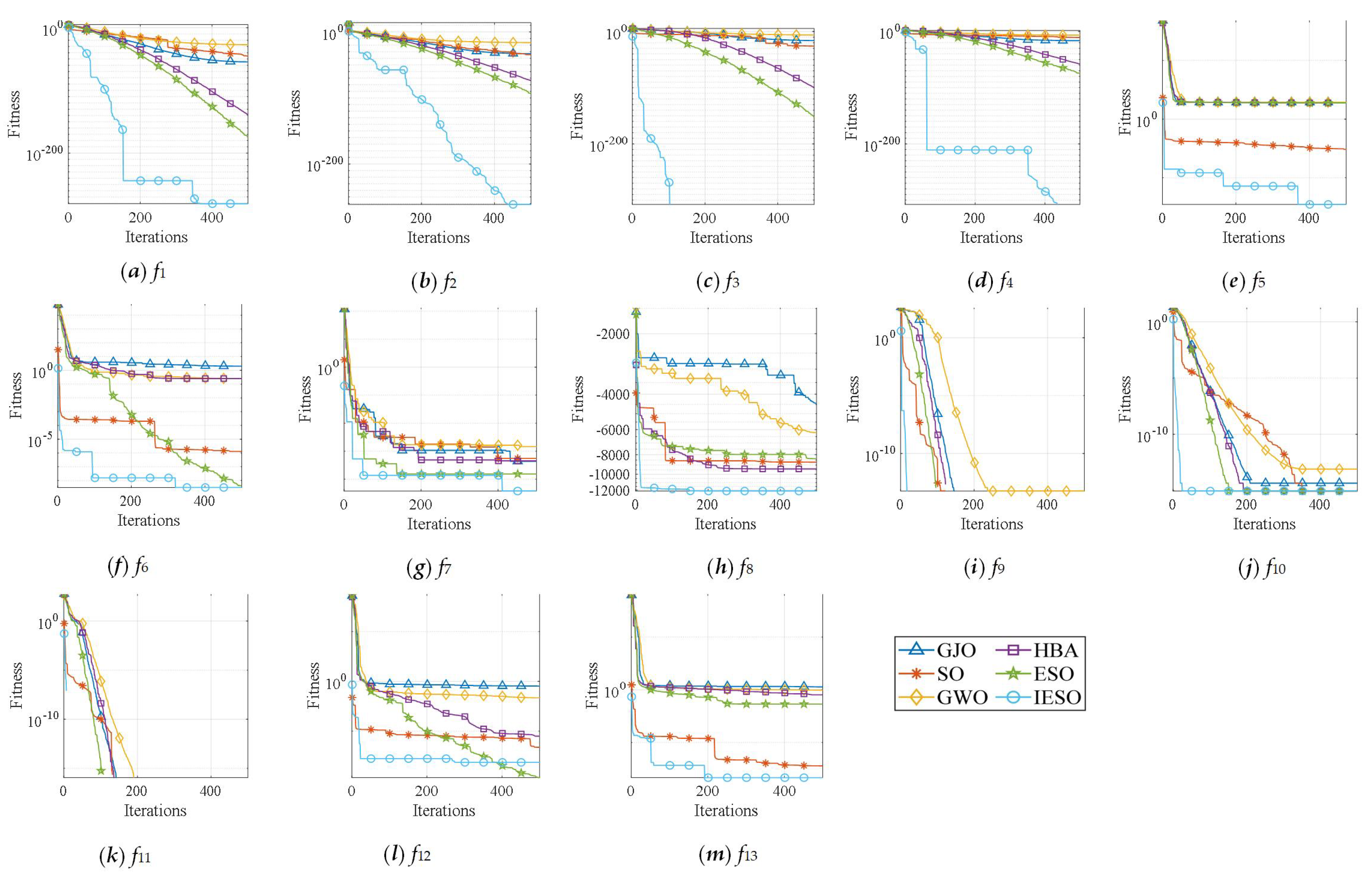
The test results across six different algorithms are summarized, with the algorithm achieving the lowest average optimization result for each test function highlighted in bold, which is shown in Table 3. In the rank-sum test, the symbols “+”, “-”, and “=” denote that IESO optimization is superior, inferior, or equivalent, respectively, compared to other algorithms. Moreover, the statistical analysis indicates that, overall, the optimization performance of IESO surpasses that of most tested algorithms. The integration of multiple strategies significantly enhances the convergence precision and stability of IESO beyond that of the standard SO, preliminarily confirming the effectiveness of these strategies. For any given test function, none of the algorithms significantly outperforms IESO. The optimization curves for various algorithms on the test function with D=1000 are illustrated in Figure 4.
Among the thirteen test functions, our IESO algorithm significantly outperforms other algorithms. This advantage is attributed to the non-monotonic decrease in the temperature factor, which fosters interaction among the foraging, combat, and mating modes. Specifically, the foraging mode utilizes the current global best position to generate high-quality solutions throughout the mid-to-high iterations, accelerating convergence. The only exception is , where ESO slightly outperforms our IESO. Its numerous local minima characterize this function, posing a considerable challenge for global optimization algorithms. The analysis suggests that introducing the mirroring mechanism has somewhat expanded the exploration horizon of the SO. However, as stated in Wang et al., [20], due to limited executions and dynamically narrowing boundaries over iterations, the development mode, which relies on information exchange between the male and female snake populations, might still result in the optimizer becoming trapped in local optima. Wang et al. suggested incorporating Lévy flights into the ESO for mutating optimal individuals. As a distinctive heavy-tailed distribution, Lévy flights, with their long and short step lengths, help the algorithm escape local optima. In our IESO, we employed a dynamic boundary to the opposite learning mechanism to enhance performance further, which has better results escaping the local optima than ESO. However, in some cases, it may not be fully utilized.
Figure 5.
Iteration fitness curves for different test functions.
A simulated digital elevation model of rugged mountainous terrain was obtained, with the map dimensions measuring 100 km by 150 km by 3 km. The maximum elevation difference in this area exceeds 2 km, featuring a terrain with significant undulations and numerous ravines. Randomly generated "no-fly zones" within this terrain are added and are illustrated in Figure 6 (purple areas). The launch point is set at coordinates (10, 90, 1.115), and the destination is at (130, 10, 1.373), with all units in kilometres (km). The fundamental challenge of path planning lies in identifying suitable waypoints during the flight to achieve an optimal flight route. To this end, this study sets 15 flight waypoints within the three-dimensional map and then employs interpolation to obtain detailed flight paths between adjacent waypoints. The parameters to be optimized are the spatial coordinates of these 15 waypoints.
The six algorithms—GJO, HBA, GWO, SO, ESO, and our IESO—were selected to plan the optimized routing on this simulated terrain. As shown in Figure 7, IESO exhibits a significantly faster convergence time than the other algorithms, at least 20% faster than GJO and over 35% faster than ESO. Additionally, Figure 8 and Figure 9 demonstrate that the route proposed by IESO is the shortest and successfully avoids all no-fly zones, as seen from both 2D and 3D perspectives. It is at least 10% shorter than the competitors. Therefore, we can conclusively state that IESO significantly improves flight planning in complex environments, such as rugged mountain terrains with substantial undulations and numerous ravines, while effectively avoiding arbitrary no-fly zones.
4. Conclusions
In this study, we propose an Improved Enhanced Snake Optimizer (IESO) to optimize 3D UAV path planning in complex conditions such as rugged mountainous terrains. The IESO refines the Enhanced Snake Optimizer (ESO) by incorporating Chebyshev chaotic mapping, a non-monotonically decreasing temperature factor, and dynamic boundary-based opposition learning (DBOL).
We validated the results in simulated experiments using thirteen different test functions under three criteria against five other innovative optimization algorithms. The IESO consistently outperformed these algorithms, demonstrating superior convergence accuracy and speed, which is over 30% shorter in distance and 10% faster in computing speed.
Author Contributions
Conceptualization, W.L. and K.Z.; methodology, W.L.; software, W.L. and Q.X.; validation, W.L., and Q.X.; formal analysis, W.L. and K.Z.; investigation, W.L.; resources, W.L. and Q.X.; data curation, X.X.; writing—original draft preparation, W.L. and X.C.; writing—review and editing, K.Z.; visualization, W.L. and K.Z.; supervision, Q.X.; project administration, Q.X.; funding acquisition, Q.X. All authors have read and agreed to the published version of the manuscript..
Funding
This work was partly supported by the Natural Science Foundation of Hunan Province under Grant NO. 2023JJ50328, and partly by the Scientific Research Project of HUAS under Grant No. 22ZD03.
Institutional Review Board Statement
Not applicable.
Data Availability Statement
The data that support the findings of this study are available on request from the corresponding author, [Wuke Li], upon reasonable request.
Conflicts of Interest
The authors declare no conflicts of interest.
Abbreviations
The following abbreviations are used in this manuscript:
| DBOL | Dynamic Boundary-based Opposition Learning |
| DOL | Dynamic Opposition Learning |
| ESO | Enhanced Snake Optimizer |
| GJO | Golden Jackal Optimization |
| GWO | Grey Wolf Optimizer |
| HBA | Honey Badger Algorithm |
| MA | Meta-heuristic Algorithm |
| SO | Snake Optimizer |
| IESO | Improved Enhanced Snake Optimizer |
| OBL | Opposition-Based Learning |
| UAV | Unmanned Aerial Vehicle |
References
- Jones, M.; Djahel, S.; Welsh, K. Path-Planning for Unmanned Aerial Vehicles with Environment Complexity Considerations: A Survey. ACM Computing Surveys 2023, 55, 1–39. [Google Scholar] [CrossRef]
- Aggarwal, S.; Kumar, N. Path planning techniques for unmanned aerial vehicles: A review, solutions, and challenges. Computer Communications 2020, 149, 270–299. [Google Scholar] [CrossRef]
- Yahia, H. S.; Mohammed, A. S. Path Planning Optimization in Unmanned Aerial Vehicles Using Metaheuristic Algorithms: A systematic review. Environmental Monitoring and Assessment 2023, 10, 10. [Google Scholar] [CrossRef] [PubMed]
- Li, D.; Yin, W.; Wong, W.E.; Jian, M.; Chau, M. Quality-oriented Hybrid Path Planning Based on A* and Q-learning for Unmanned Aerial Vehicle. IEEE Access 2021, 10, 7664–7674. [Google Scholar] [CrossRef]
- Pan, Z.; Zhang, C.; Xia, Y.; Xiong, H.; Shao, X. An Improved Artificial Potential Field Method for Path Planning and Formation Control of the Multi-UAV Systems. IEEE Transactions on Circuits and Systems II: Express Briefs 2022, 69, 1129–1133. [Google Scholar] [CrossRef]
- Wang, J.; Li, Y.; Li, R.; Chen, H.; Chu, K. Trajectory Planning for UAV Navigation in Dynamic Environments with Matrix Alignment Dijkstra. Application of soft computing 2022, 26, 12599–12610. [Google Scholar] [CrossRef]
- Prasad, N. L, Ramkumar, B. 3-D Deployment and Trajectory Planning for Relay Based UAV Assisted Cooperative Communication for Emergency Scenarios Using Dijkstra’s Algorithm. IEEE Transactions on Vehicular Technology 2022, 72, 5049–5063. [Google Scholar] [CrossRef]
- Flores-Caballero, G. , Rodríguez-Molina, A., Aldape-Pérez, M., Villarreal-Cervantes, M. G. Optimized Path-Planning in Continuous Spaces for Unmanned Aerial Vehicles Using Meta-Heuristics. IEEE Access 2020, 8, 176774–176788. [Google Scholar] [CrossRef]
- Shao, S. , He, C., Zhao, Y., Wu, X. Efficient Trajectory Planning for UAVs Using Hierarchical Optimization. IEEE Access 2021, 9, 60668–60681. [Google Scholar] [CrossRef]
- Chen, J. C. , Ling, F. Y., Zhang, Y., You, T., Liu, Y. F., Du, X. Y. Coverage Path Planning of Heterogeneous Unmanned Aerial Vehicles Based on Ant Colony System. Swarm and Evolutionary Computation 2022, 69, 101005. [Google Scholar] [CrossRef]
- Yao, L. , Yuan, P., Tsai, C.Y., Zhang, T., Lu, Y., Ding, S. ESO: An Enhanced Snake Optimizer for Real-world Engineering Problems. Expert Systems with Applications 2023, 230, 120594. [Google Scholar] [CrossRef]
- Hashim, F.A. , Hussien, A.G. Snake Optimizer: A Novel Meta-heuristic Optimization Algorithm. Expert Systems with Applications 2022, 242, 108320. [Google Scholar] [CrossRef]
- Wolpert, D.H. , Macready, W.G. No Free Lunch Theorems for Optimization. IEEE Transactions on Evolutionary Computation 1997, 1, 67–82. [Google Scholar] [CrossRef]
- Chopra, N. , Ansari, M.M. Golden Jackal Optimization: A Novel Nature-inspired Optimizer for Engineering Applications. Expert Systems with Applications 2022, 198, 198. [Google Scholar] [CrossRef]
- Hashim, F.A. , Houssein, E.H., Hussain, K., Mabrouk, M.S., Al-Atabany, W. Honey Badger Algorithm: New Metaheuristic Algorithm for Solving Optimization Problems. Mathematics and Computers in Simulation 2022, 192, 84–110. [Google Scholar] [CrossRef]
- Nadimi-Shahraki, M. , Taghian S., Mirjalili S. An Improved Grey Wolf Optimizer for Solving Engineering Problems. Expert Systems with Applications 2021, 166, 113917. [Google Scholar] [CrossRef]
- Xu, Y. , Li, X., Yang, J., Zhang, D. Integrate the original face image and its mirror image for face recognition. Neurocomputing 2014, 131, 191–199. [Google Scholar] [CrossRef]
- Tizhoosh, H. R. Opposition-based learning: a new scheme for machine intelligence. International conference on computational intelligence for modelling, control and automation and international conference on intelligent agents, web technologies and internet commerce (CIMCA-IAWTIC’06) 2005, 131, 695–701. [Google Scholar] [CrossRef]
- Wu, T.Y. , Li, H., Chu, S.C. CPPE: An Improved Phasmatodea Population Evolution Algorithm with Chaotic Maps. Mathematics 2023, 11, 1977. [Google Scholar] [CrossRef]
- 16. Wang, C., Jiao, S., Li, Y. and Zhang, Q. Capacity Optimization of a Hybrid Energy Storage System Considering Wind-Solar Reliability Evaluation Based on A Novel Multi-strategy Snake Optimization Algorithm Expert Systems with Applications 2023, 231, 120602. [CrossRef]
Figure 1.
IESO Flowchart
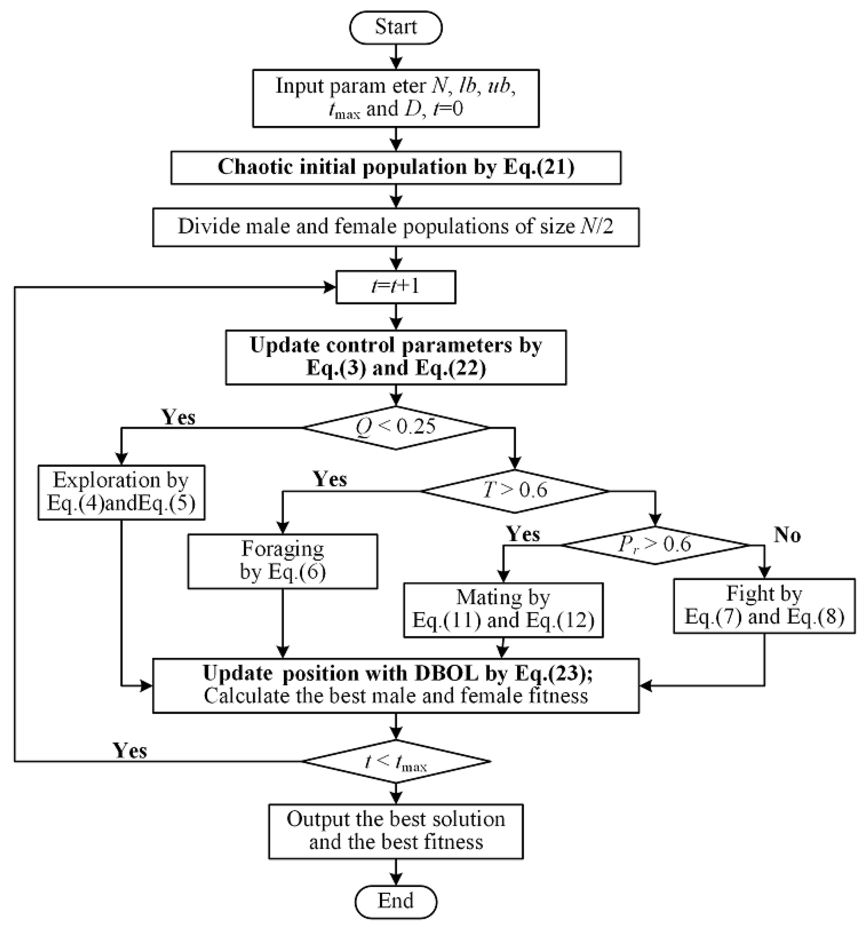
Figure 2.
Initial value distribution by (a) Normal Random distribution and (b) Chebyeshev Chaotic map.
Figure 2.
Initial value distribution by (a) Normal Random distribution and (b) Chebyeshev Chaotic map.
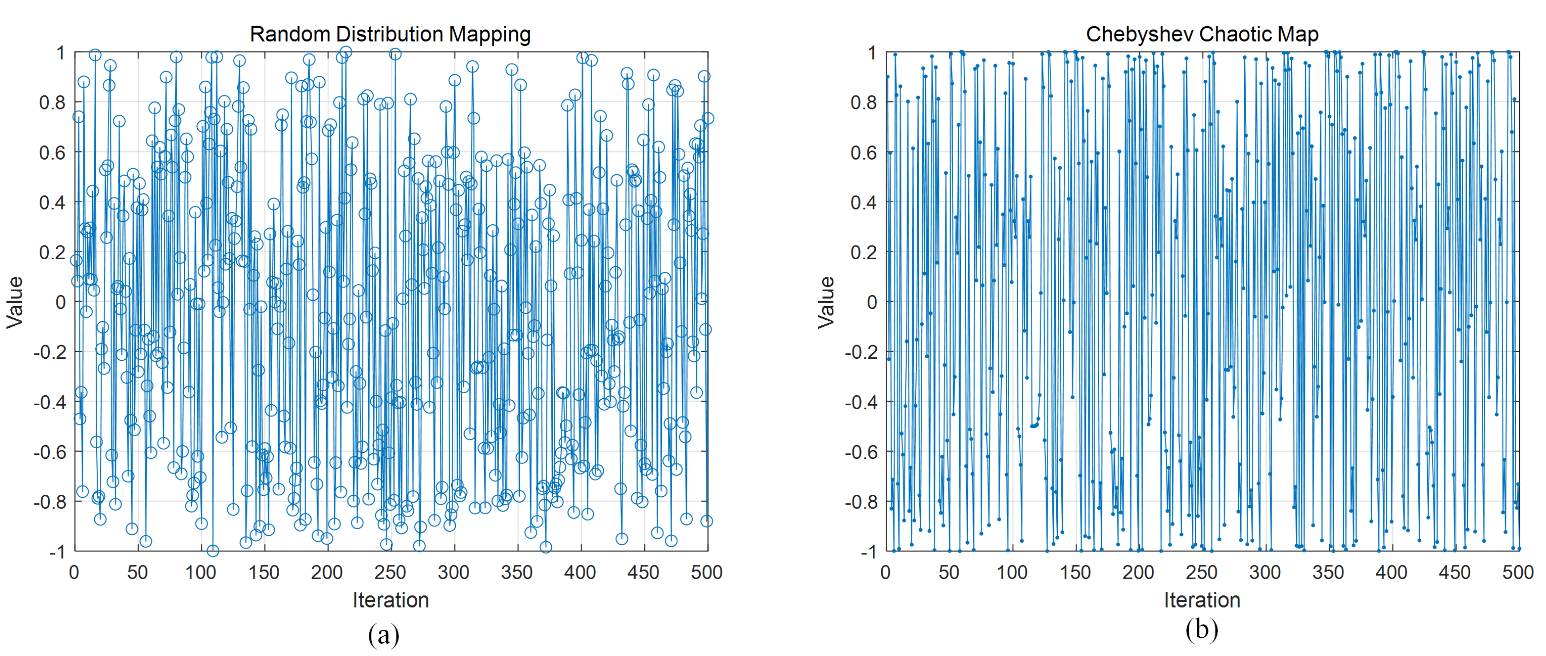
Figure 6.
The simulated rugged mountain terrain with "no-fly" zones.
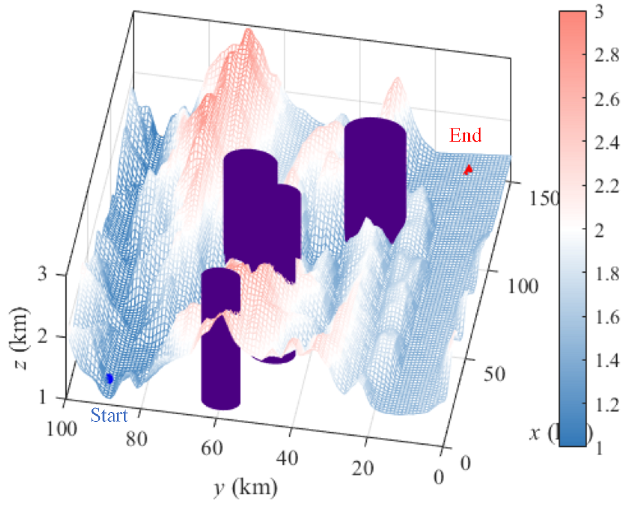
Figure 7.
Iteration fitness curves for the six algorithms
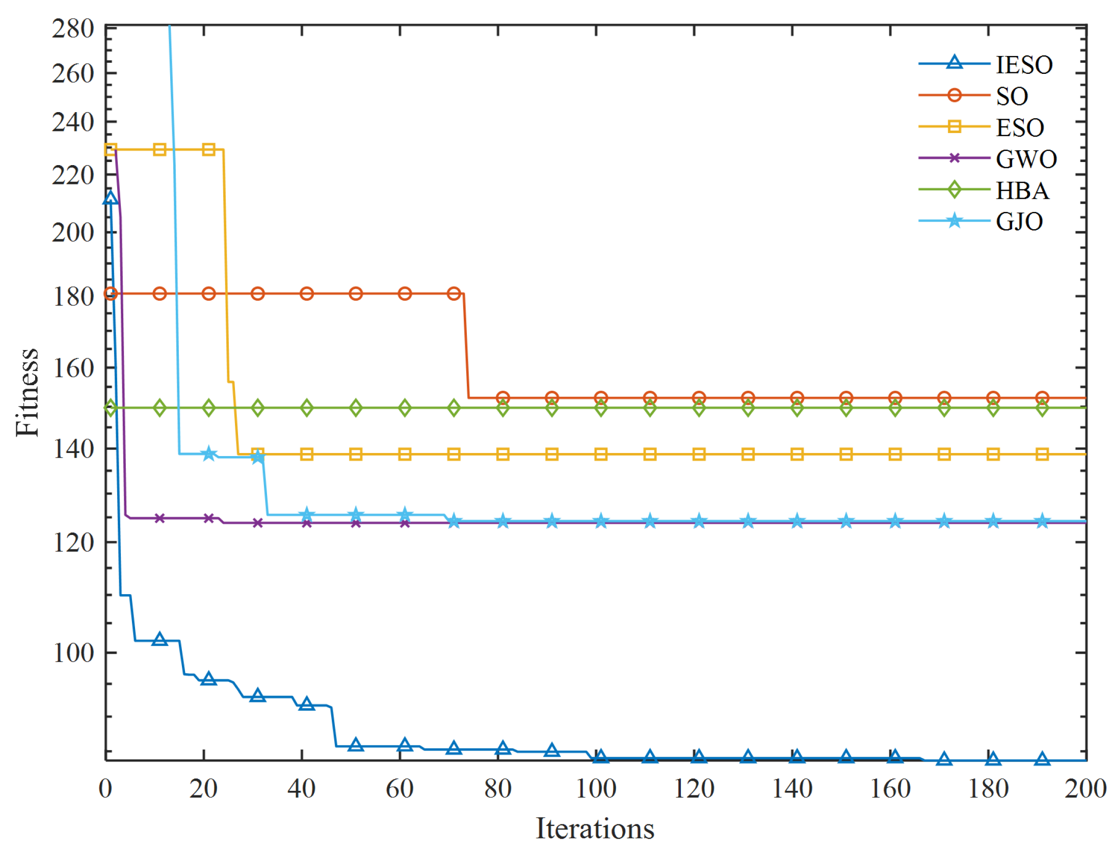
Figure 8.
The planned routes from the six algorithms
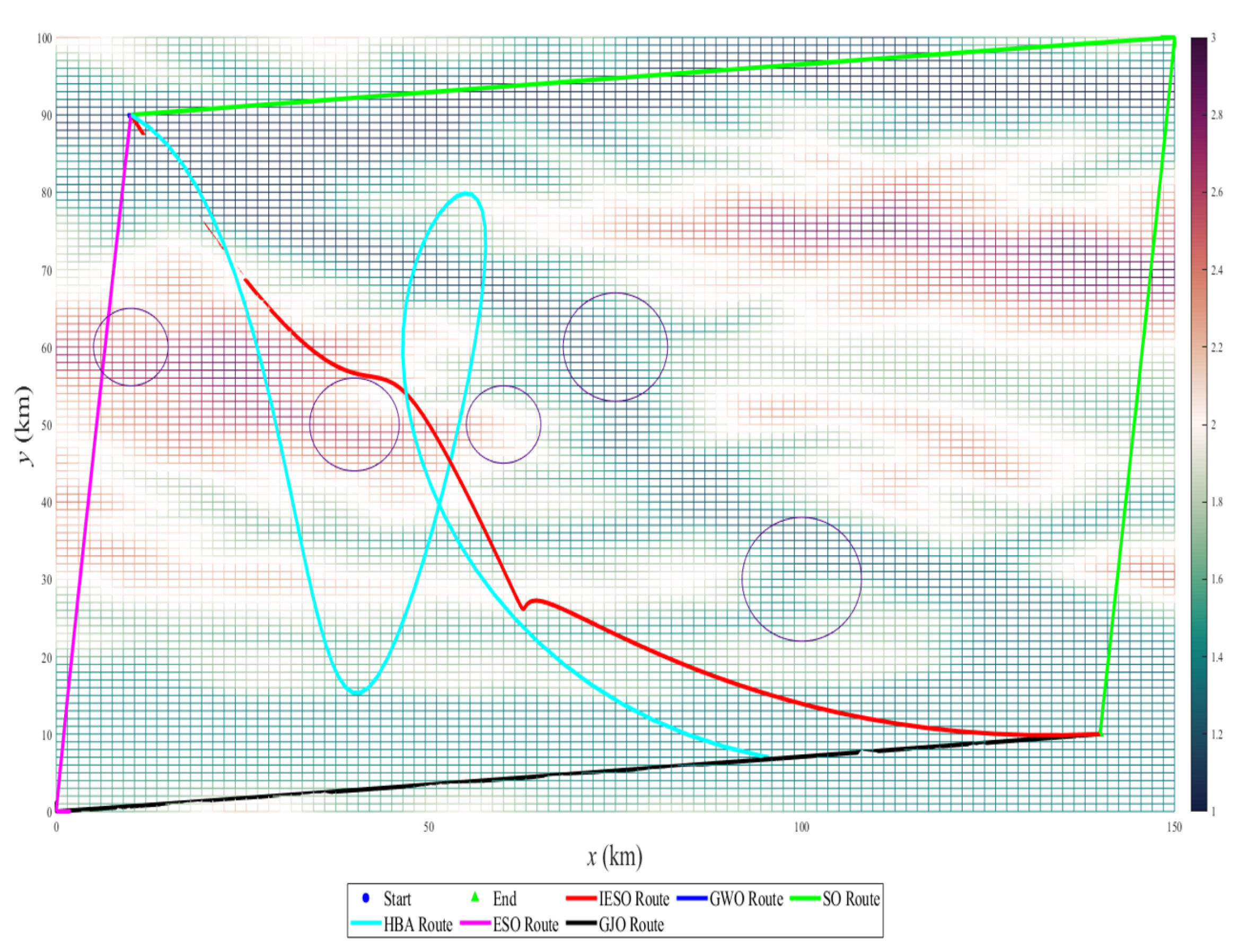
Figure 9.
The IESO planned route on the simulated terrain
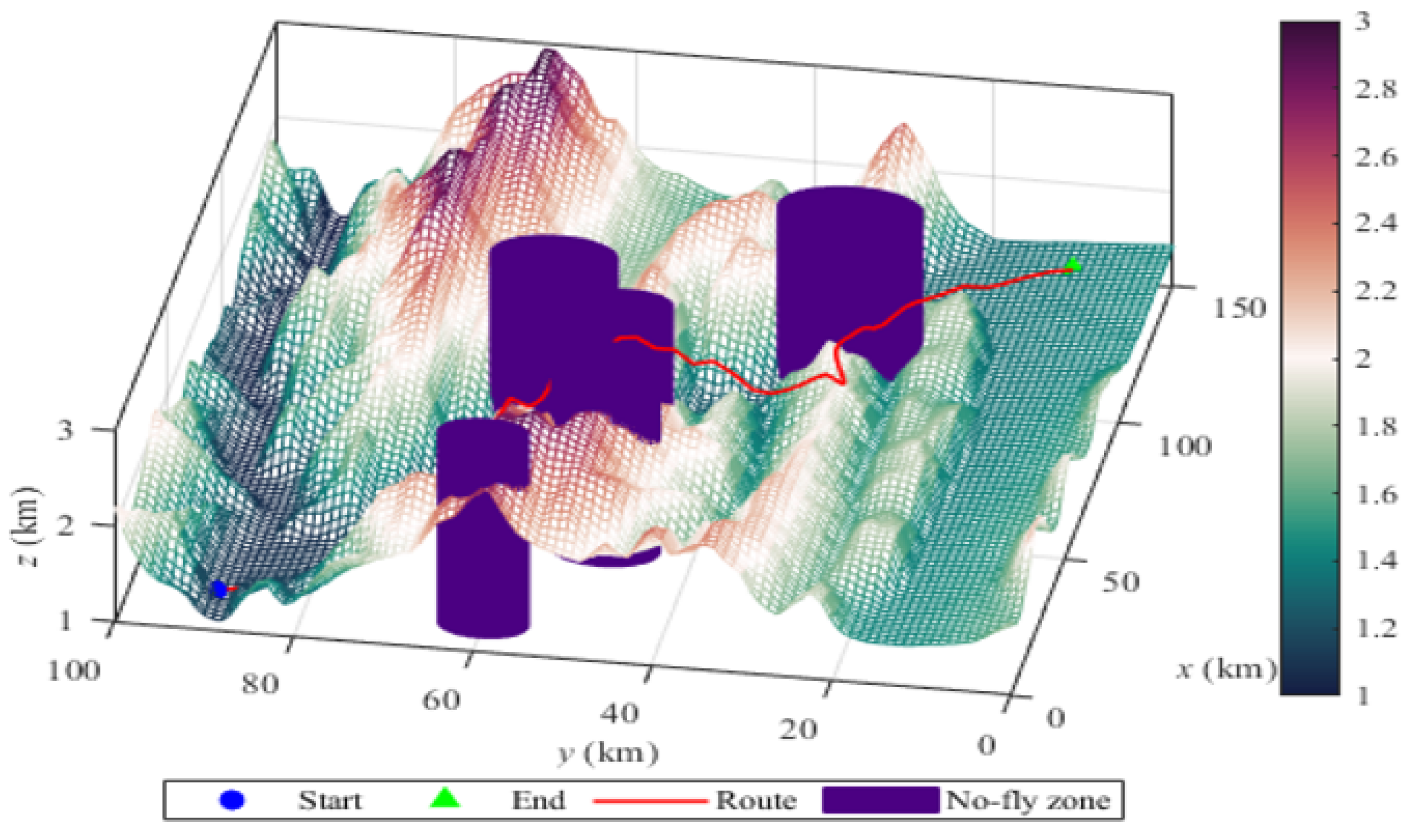

Table 1.
Formula and parameters of 13 benchmark test functions.
| Num. | Name | Formula | Range | |
|---|---|---|---|---|
| Sphere’s Function | [-100,100] | 0 | ||
| Schwefel’s Problem 2.22 | [-10,10] | 0 | ||
| Schwefel’s Problem 1.2 | [-100,100] | 0 | ||
| Schwefel’s Problem 2.21 | [-100,100] | 0 | ||
| Generalized Rosenbrock’s Function | [-30,30] | 0 | ||
| Step Function | [-100,100] | 0 | ||
| Quartic Function | [-1.28,1.28] | 0 | ||
| Generalized Schwefel’s Problem 2.26 | [-500,500] | -2094 | ||
| Generalized Rastrigin’s Function | [-10,10] | 0 | ||
| Ackley’s Function | [-10,10] | 0 | ||
| Generalized Griewank’s Function | [-10,10] | 0 | ||
| Generalized Penalized Function 1 | [-10,10] | 0 | ||
| Generalized Penalized Function 2 | [-10,10] | 0 |
Table 2.
Algorithm parameters.
| Algorithms | Parameters |
|---|---|
| IESO | |
| ESO | |
| SO | |
| GJO | |
| HBA | |
| GWO |
Table 3.
Test results of 13 benchmark functions (D=1000)
| Num. | GJO | SO | GWO | HBA | ESO | IESO |
|---|---|---|---|---|---|---|
| 5.76E-55(7.15E-55)/+ | 9.32E-37(2.69E-36)/+ | 9.32E-28(2.82E-28)/+ | 5.00E-137(7.43E-137)/+ | 3.38E-197(0.00E+00)/+ | 0.00E-00(0.00E-00) | |
| 1.29E-32(1.18E-32)/+ | 6.02E-34(1.75E-33)/+ | 6.02E-17(1.27E-16)/+ | 4.20E-72(9.64E-72)/+ | 5.40E-92(1.45E-91)/+ | 7.52E-240(0.00E-00) | |
| 1.37E-17(2.54E-17)/+ | 9.89E-17(1.69E-17)/+ | 9.89E-06(6.81E-07)/+ | 2.81E-101(4.02E-101)/+ | 1.10E-150(2.94E-150)/+ | 0.00E-00(0.00E-00) | |
| 2.75E-16(7.85E-16)/+ | 7.57E-09(1.25E-08)/+ | 7.57E-07(7.28E-07)/+ | 2.47.00E-137(7.43E-137)/+ | 2.35E-197(6.41E-77)/+ | 7.88E-135(2.94E-134) | |
| 2.75E+01(7.85E-01)/+ | 7.57E-03(1.25E-03)/+ | 2.43E-01(7.28E-01)/+ | 2.47E-137(7.43E-137)/+ | 2.35E-197(6.41E-01)/+ | 1.21E-07(1.64E-06) | |
| 2.76E-04(3.82E-01)/+ | 3.10E-05(5.92E-05)/+ | 3.10E-28(2.82E-02)/+ | 2.56E-137(7.43E-137)/+ | 2.79E-197(7.51E-02)/+ | 9.52E-08(1.08E-08) | |
| 2.95E-55(1.66E-04)/+ | 4.96E-03(3.33E-04)/+ | 4.96E-28(2.82E-04)/+ | 2.85E-137(7.43E-137)/+ | 1.85E-197(1.88E-04)/+ | 1.82E-04(1.03E-04) | |
| -3.70E+03(1.04E+03)/+ | -9.70E+03(2.27E+03)/+ | -9.70E-28(8.73E+02)/+ | -9.02E-137(7.43E-137)/+ | -8.62E+03(0.00E-00)/+ | -1.08E+04(1.38E+03) | |
| 0.00E-00(0.00E-00)/= | 0.00E-00(0.00E-00)/= | 2.18E-02(5.68E-14)/+ | 0.00E-00(0.00E-00)/= | 0.00E-00(0.00E-00)/= | 0.00E-00(0.00E-00) | |
| 6.13E-55(1.83E-15)/+ | 1.87E-15(2.48E-15)/+ | 1.86E-13(1.48E-14)/+ | 8.88E-00(0.00E-00)/= | 8.88E-16(0.00E-00)/= | 8.88E-16(0.00E-00) | |
| 0.00E-00(0.00E-00)/= | 0.00E-00(0.00E-00)/= | 0.00E-00(0.00E-00)/= | 0.00E-00(0.00E-00)/= | 0.00E-00(0.00E-00)/= | 0.00E-00(0.00E-00) | |
| 2.95E-02(1.66E-02)/+ | 4.96E-07(3.33E-07)/+ | 4.96E-02(7.30E-02)/+ | 2.85E-04(1.78E-03)/+ | 1.85E-09(5.88E-09)/= | 2.53E-09(3.26E-09) | |
| 1.75E-00(2.20E-01)/+ | 2.98E-05(8.17E-05)/+ | 2.95E-05(1.74E-01)/+ | 3.80E-01(2.76E-01)/+ | 1.43E-01(1.72E-01)/+ | 7.13E-08(7.36E-08) | |
| Wilcoxon Test Summary | 12/1/0 | 10/3/0 | 12/1/0 | 9/4/0 | 8/5/0 | Wilcoxon |
* The data format: Average / Standard Deviation / Wilcoxon Test Sign (+/-/=)
Disclaimer/Publisher’s Note: The statements, opinions and data contained in all publications are solely those of the individual author(s) and contributor(s) and not of MDPI and/or the editor(s). MDPI and/or the editor(s) disclaim responsibility for any injury to people or property resulting from any ideas, methods, instructions or products referred to in the content. |
© 2024 by the authors. Licensee MDPI, Basel, Switzerland. This article is an open access article distributed under the terms and conditions of the Creative Commons Attribution (CC BY) license (http://creativecommons.org/licenses/by/4.0/).
Copyright: This open access article is published under a Creative Commons CC BY 4.0 license, which permit the free download, distribution, and reuse, provided that the author and preprint are cited in any reuse.


