
Submitted:
27 May 2025
Posted:
28 May 2025
You are already at the latest version
Abstract
Fish coloration plays an important role in reproduction and camouflage, yet capturing color variation in field conditions remains challenging. We present a standardized, semi-automated protocol for measuring body coloration in the popular model fish threespine stickleback (Gasterosteus aculeatus). Individuals are photographed in a controlled light box within minutes of capture, and color is sampled from eight anatomically defined standard sites in human-perception–based CIELAB space. Analyses combine univariate color metrics, multivariate statistics, and the ΔE* perceptual difference index to detect subtle shifts in hue and brightness. Validation on laboratory-reared and wild-caught pre-spawning fish shows the method reliably distinguishes males and females well before full breeding colors develop. Although it currently omits ultraviolet signals and fine-scale patterning, the approach scales efficiently to large sample sizes and varying lighting conditions, making it well suited for population-level surveys of camouflage dynamics, sexual dimorphism, and environmental influences on coloration in sticklebacks and other fish species.
Keywords:
threespine stickleback
; sexual dimorphism
; body coloration
; coloration measurements
; White Sea
1. Introduction
Fish coloration patterns are in focus of numerous studies of marine and freshwater taxa and utilizing broad range of methods [1,2,3,4,5]. These studies are often based on water pool experiments, yet field direct observational datasets are also common. Studies of coloration in model fish species including zebrafish, guppies, cichlids and threespine stickleback have further enabled detailed investigations of physiology and genetics of coloration [6,7,8,9,10,11,12,13,14,15,16,17].
Fish body coloration serves as a versatile communication channel, closely tied to both behavior and environmental contexts [18,19]. Weather through disruptive or countershading camouflage that helps prey avoid predators [20], or vivid nuptial displays that attract mates during spawning [21], coloration underpins key ecological and evolutionary processes. Even in pelagic species inhabiting relatively homogenous environments, variable body coloration, controlled by specialized light-reflecting and polarizing cell structures, provides adaptive camouflage [8,22].
The threespine stickleback Gasterosteus aculeatus L. is a popular model species in behavioral and evolutionary biology due to ecological plasticity, high abundances, and ability to thrive in aquaria experiments. Among the well-known features of the life history of G. aculeatus is color dimorphism during the spawning season, when males become reddish with orange hues and blue eyes, and females mostly remaining cryptically colored [23,24]. Studies of nesting behavior in male stickleback demonstrated the adaptive role of nuptial coloration in sexual selection and speciation [25], and have demonstrated that ultraviolet cues are important signals in communication among sticklebacks [15,26,27]. In threespine stickleback, variation in spatial distribution and grouping of melanophores, including e.g., the formation of vertical stripes in the rear part of the body is likely linked to camouflage coloration important for the adaptation to contrasting niches [28,29].
Quantifying the nuptial coloration has evolved from simple visual scales assigning discrete visual red-colored gradients [26,30] to calculating photographic “redness indices” by measuring relative contribution of red, green and blue in RGB color space [31], segmenting colored pixels [32,33], or using spectrophotometry to derive hue, chroma, and brightness from reflectance spectra [25,34]. Further development of methods included focusing on specific landmarks across the body [35].
In the seas, sticklebacks spend the non-breeding season in offshore habitats, displaying only cryptic pelagic coloration in both males and females. For spawning, sticklebacks migrate to coastal habitats and streams with a higher proportion of nests being built among the vegetation. Thus, males form a combination of nuptial and camouflage coloration patterns at spawning coastal grounds to avoid predation and be ready to display when courtship begins. The female stickleback coloration also shifts with maturity stage, yet has received less attention from researchers despite its potential contribution to evidence affecting mating and nest defense.
In the subarctic White Sea, which we used as a source of material, abundance of sticklebacks on spawning grounds now often exceeds 100 individuals per m², with the sex ratio of around two females per male [36,37,38]. Nevertheless, only three nests per m² are being built (M. Ivanov, unpublished) [39], thus, only a fraction of males and females can spawn at once. The likely consequence of this is different hormonal levels of fish which may manifest in individual nuptial coloration intensity. In particularly, the observed very high egg cannibalism [40,41] could drive high turnover among both sexes, which thus may result in their variation in coloration patterns.
Despite the range of techniques available for studying stickleback coloration, none readily capture the full complexity of population-level dynamics. Simple visual scores or single-spot measurements may record obvious nuptial flashes or broad camouflage patterns, but they cannot accommodate the mixtures of faint pre-spawning hues, cryptic coloration patterns, and bright breeding colors that often coexist within a single fish and vary with habitat. Likewise, laboratory-based spectrometry and landmark-sampling methods lack the flexibility required for large-scale surveys of hundreds of individuals under changing light, background, and behavioral conditions.
In this study, we aim to develop a universal technique for quantifying coloration in population studies of G. aculeatus. Our goal was a method that (1) is sensitive enough to detect the earliest male or female color cues before spawning, (2) can track color shifts in fish during the spawning season, and (3) scales to large field datasets without reduction precision.
We validated this technique on two datasets in which sex-specific coloration is not immediately apparent: on fish maintained under standard laboratory conditions, and on fish sampled immediately upon capture in the wild. Specifically, we asked the following questions: (i) Can our method reliably distinguish males from females by coloration during the pre-spawning period? (ii) Which body regions provide the strongest discrimination between sexes? (iii) Which coloration components contribute most to these differences?
2. Materials and Methods
The study was conducted at the Educational and research station "Belomorskaia" of Saint Petersburg State University, located in the Kandalaksha Bay of the White Sea (66°17.606' N, 33°38.747' E). A beach seine measuring 7x1.5 m was used to catch fish in the Seldianaya Inlet on June 5, 2021, three days after the first sticklebacks were observed in the inshore zone, following their inshore migration from the open waters where they had wintered. At that time of capture, spawning coloration was not observed. In the White Sea, the usual body length from the end of the snout to the beginning of the rays of the tail fin, AD (or SL, standard length), is 57.5 mm for males 62.8 mm for females [37]. Fishes from 1+ to 5+ years old can be present at the spawning grounds; however, the population is most often composed of 2-year-old specimens [36,42]. Approximately 1,100 specimens (with an estimated sex ratio of 1 male to 2 females) were placed in a pool with dimensions of 2.5 x 1.5 x 0.6 m without spawning substrate, and the water temperature maintained around 12°C under natural photoperiod conditions (around the clock light). The fish were regularly fed with TetraMin® granules (Spectrum Brands, Germany). All sticklebacks were kept in these conditions for 11 days before the experiment. We placed fish in experimental conditions that offset physiological and morphological factors of color change in order to avoid the influence of environmental heterogeneity. No breeding behavior was recorded during this experiment.
Eleven days after the capture, 34 females and 17 males were randomly selected for analysis. Generally, marine White Sea stickleback females are larger, have smaller heads and more fusiform body shapes than males (see [43] for detailed characteristics of sexual dimorphism). Males and females can also be distinguished by their inner mouth color: males have bright orange lips, while females have pale lips. Thus, sex was determined by morphological traits and then verified through dissections of all specimens.
We also sampled wild fish from the Seldianaya Inlet (66°20.284' N, 33°37.354' E) on June 04, 2023 four days after the sticklebacks migrated to the nearshore areas but still before males started the nest building. The sample consisted of 30 males and 30 females which were characterized by lack of spawning coloration signs.
Each individual was photographed alive in a specially designed wooden photo box measuring 60 x 60 x 60 cm in 1-2 minutes after the capture. The box was painted with white matte paint both inside and out. Two AA-cell bracket lights were used for lighting. The photos were taken with a Canon EOS 650D DSLR camera (f=18 mm using ISO=100) and RICOH WG-6 (f=4.2, ISO variable). The camera was positioned perpendicular to the shooting plane with the lens facing downwards, always 17 cm from the photographed surface. This setup, with fish placed in the center of the box just after capture (5 specimens per series), helped reduce distortion at the edges of the image and ensured accurate size representation of the photographed objects (Figure 1). Pictures were taken in. RAW format with an image size of 3456 x 5184 pixels using EOS D650D and in .jpeg using RICOH WG-6 (image size 5184 х 3888 pixels). In the resulting images, the pixel to mm ratios were 18:1 for D650D and 24:1 for WG-6. For color corrections, we used Datacolor SpyderCheckr24 color card, followed by processing in Adobe Lightroom [44] and SpyderCheckr 1.3 software [45]. Corrected images were saved in .JPEG format and analyzed using ImageJ software [46,47].
Measurements of fish body coloration were conducted using CIELAB color space, where L* represents lightness, ranging from 0 (black) to 100 (white), a* represents the green to magenta parameter, ranging from -100 (fully green) to +100 (fully magenta), and b* represents the blue to yellow parameter, ranging from -100 (fully blue) to +100 (fully yellow). Combination of L=50, a*=0 and b*=0 mean a point of neutral gray [48,49,50]. General color description in this color space is presented in Figure S1. This model was chosen because it aligns with human perception of color, rather than the fish's visual apparatus. Prior studies of fish color variability, including mating coloration in male sticklebacks, have also relied on human perception [51,52,53].
Color parameters L*, a*, and b* were measured using ImageJ software [46,47] following three steps. First, the image was split into three channels — L*, a*, b* — through the Image menu (full path: Image – Type – Lab stack). Regions of interest, hereafter mentioned as standard sites (SS) were selected using the built-in Rectangle tool, and a set of regions was created using the Region of interest Manager tool. In this study, each standard site (SS) was a 20x20 pixel square, representing the average of 400 pixels, in metric units this square had a side of approximately 1.07 mm and an area of 1.14 mm2. The values for each SS in the three channels were measured using the micaToolbox plugin [54]. To mitigate potential distortion of luminosity data due to glare, adjustments to the SS location were permitted within a 60x60 pixel area when glare was detected.
To estimate the per-site pairwise differences in total color change between males and females, and between experiment and field dataset, ΔE* pigmentation index was calculated using formula:
where L*, a* and b* are values of CIELAB chromatic parameters in pairwise comparisons.
For each SS, mean values of color coordinates were used for ΔE* calculation. Distances between colors were considered based on ΔE* values: irrelevantly perceptually different (ΔE* < 1), slightly perceptually different (1 < ΔE* < 2.3) or clearly perceptually different (ΔE* > 2.3) [55]. For interpreting results, the smallest perceivable difference between the colored patches is considered as 0.5–1.0 ΔE units.
Statistical analyses were conducted using PAST 5.2.2 [56], JASP 0.19.3.0 [57], Python 3.13 [58] in Anaconda Navigator software [59] and R 4.5.0 [60] in RStudio [61]. The distribution of all parameters (L*, a* and b*) differs from normal in some cases (Shapiro-Wilk test, p<0.05), thus we use Mann-Whitney test to compare means from samples with non-normal distribution and Student’s t-test when comparing means from samples with normal distribution. From this point on, any differences for which the p-value is p<0.05 will be mentioned as significant.
Principal component analysis (PCA) was performed to check the hypothesis whether there is sexual dimorphism in body coloration. To perform the analysis, we transformed the data following these algorithms. Firstly, both for a* and b* metrics we add +100 units to avoid negative values. Then each coloration metric values (L*, a*, b*) were standardized across individuals for each standard site (SS), i.e., we generate a dataset consisting of deviations from the mean and standard deviation units. This involved calculating the mean and standard deviation for L*, a*, and b* values for each SS, and adjusting individual coloration values accordingly. Once standardized, means or medians (if distribution is not normal) based on all SSs were calculated for each SS within each individual, and PCA performed based on these means.
3. Results
3.1. Method Developing: Standard Sites Selection and Coloration Description
To describe the stickleback coloration patterns, we identified eight standard sites (SS) located on different parts of the body (Figure 2). These SS were selected taking into account five criteria: (i) variability of coloration intensity across the body, (ii) variability of male coloration during the breeding season, (iii) differences in coloration between males and females during the breeding season, (iv) suitability for measurements on two-dimensional computer images, and (v) practicality to ensure that the analysis would not be excessively labor-intensive. In selecting the SS, we considered both gradient areas (as in [62]) and threespine stickleback-specific coloration patterns ([27,63,64] and references therein).
3.2. L*, a* and b* Variation
3.2.1. Lightness (L*)
In the experimental dataset, color parameter L* parameter show the range in females from 11.3 to 84.3, among the SS in focus and studied individuals; in males L* varied from 3.7 to 69.5. The darkest SS – SS1, located close to the dorsum, this was observed in both sexes: in females mean L* was 22.1±4.7 (mean±SD) and for males – 20.4±5.0 (Figure 3). Low L* values were also found at the eye iris (SS6 and SS7); for females the mean 34.1±11.2 and 35.5±7.4 for SS6 and SS7 respectively and for males these mean values are 18.1±8.3 and 22.3±10.3 respectively. Conversely, the lightest areas were found on the midbody (SS2, SS4) and abdomen (SS3, SS5), with L* mean values ranging from 34.6±7.4 to 55.8±6.6 in females and from 35.9±7.1 to 51.7±7.2 in males. Females generally demonstrated higher lightness (L*) values compared to males. This trend was consistent across the multiple SS, particularly cryptic SS such as SS1 (dorsal side) and SS3 (ventral side).
In the field dataset, the overall L* parameter in females varied from 12.80 to 66.79, in males – from 8.1 to 62.9. Both females and males have brighter sex-related SS such as SS4 (mean for females was 54.9±5.5 and for males – 51.2±7.8), SS5 (mean for females was 60.4±2.5 and for males – 55.2±9.6) and SS6 (mean for females was 44.3±8.9 and for males – 25.0±8.7). The group of darker SSs slightly differ, because the lowest L* value for females was in dorsum (SS1) with mean 17.6±2.4, while males have not only darker dorsum (SS1) with mean 20.4±7.3, but also the iris (SS6 and SS7, means 25.0±8.7and 24.4±10.9, respectively). Pair comparison reveals significantly different values between sexes for SS5, SS6 and SS7, what can be seen at Figure 3. No obvious patterns are registered for groups of sex-related and cryptic coloration SS.
All detailed information on the mean values for each SS for L* and other two CIELAB parameters and results of pair comparisons for males and females both for experimental and field data can be found at Table S1. In further description we do not use this reference.
3.2.2. Green to Magenta Axis (a*)
In the experimental dataset, parameter a* varied from -6.8 to 10.3 in females and from -9.1 to 4.6 in males. Females demonstrated a pronounced shift toward magenta at specific SS, notably the iris (SS6, SS7), operculum (SS4), and preoperculum (SS5), and the variation of means between all these SS was from 3.6±1.1to 5.3±1.8, while a shift toward green coloration is observed on the dorsum (SS1) – the mean was -0.6±2.2. Males predominantly manifested greenish tints (negative a* values), particularly on the frontal body parts (SS4, SS6, SS8), with their means ranged from -2.4±1.8 to -1.9±2.9 (see Table S1 and Figure 4). Coloration between females and males significantly differs between all the SS, except for SS1.
The range of the a* parameter in females from the field conditions covered positive and negative values with the minimum of -5.0 and the maximum of 6.2. In males from the field conditions, the range was slightly shifted to the greenish colors with the minimum of -6.9 and the maximum of 2.4. All mean values from cryptic coloration SS (SS1, SS2, SS3 and SS8) were below zero, i.e., slightly shifted to the greener colors, with the mean values ranged between -2.8±1.3 and -0.8±0.9 in females and between -4.2±1.3 to -1.4±1.5 in males. Mean values of sex-related coloration SS for both sexes tended to be less greenish, e.g., means in females ranged from -1.6±1.1 to 1.4±2.1 and in males – from -2.4±1.9 to -0.4±1.4. In addition, pair color comparison demonstrated significant differences in males and females a* mean values for all SS, except for SS1 (see Figure 4). When comparing sex-related and cryptic coloration SS, there were not found any clear patterns.
3.2.3. Blue to Yellow Axis (b*)
Within experimental data, values for the b* parameter (Figure 5) in females ranged from 1.0 to 27.8, and in males – from -6.9 to 31.4. In females, a distinct yellow shift was noted at several SS, including the dorsum (SS1, SS8), lateral side (SS2), operculum (SS4), and iris (SS6) – mean values on these SS varied from 14.7±2.9 to 19.2±4.4. In males, a general yellow shift was observed across the six different SS with the means from 15.9±3.6to 20.7±7.0. However, the iris on males was slightly blue-shifted with means 7.4±8.9 (SS6) and 10.8±5.2 (SS7). Some significant differences between males and females were found for the six SS: SS2, SS3, SS4, SS5 and SS6.
Across the field data the following results were obtained. The b* values for females had the minimum of -3.7 and the maximum of 23.0, but all the mean values were positive. The most yellow-shifted SS were SS8 (mean 14.0±3.2), SS2 (mean 12.6±3.9) and SS3 (mean 11.1±3.2). For males b* parameter values ranged from -2.2 to 27.8, and all the means were also positive (Figure 5). They had five most yellow-shifted SS such as SS8 (mean 15.9±5.8, SS2 (mean 14.9±6.3), SS3 (mean 13.6±4.8), SS4 (mean 13.6±6.4) and SS5 (mean 11.2±4.8). Statistically significant differences between males and females were among the following SS (in a range from the maximum to minimum mean values): SS3, SS4, SS5 and SS1 (Figure 6).
3.3. Principal Component Analysis
Ordination of individual fish color profiles L*, a*, b* indicated the presence of four groups broadly separating males and females within experimental and field datasets. According to the PCA results, groups of points were well segregated with a slight overlap between two groups of males, and a slight overlap between males and females from the field conditions (Figure 7). The first component (PC1) explained 26.1% of the total variation, the second component (PC2) – 22.0%, and the third component (PC3) – 14.7. Loadings along PC1 for three parameters L*, a* and b* were 0.2, 0.8 and 0.03 respectively. Loadings along PC2 were -0.2 for L*, 0.05 for a* and 0.7 for b*. Overall loadings along PC3 were 0.5 for L*, -0.2 for a* and 0.2 for b*. This means that PC1 was positively correlated with a* parameter variability, PC2 described b* alteration, while PC3 was slightly connected with L* variability. According to t-test, significant differences in PCA scores between females from the two groups were found only along PC1 (t=11.96, p<0.001, critical t-value (p=0.05) =1.999) and PC2 (t=11.57, p<0.001, critical t-value (p=0.05) =1.999). However, males demonstrated significant difference for PC1 (t=2.37, p=0.02, critical t-value (p=0.05) =2.01), PC2 (t=7.398, p<0.001, critical t-value (p=0.05) =2.01) and PC3 (t=2.21, p=0.03, critical t-value (p=0.05) =2.01). In addition, we observed positive correlations between a* parameters and PC1, positive correlations between parameter b* and PC2 and positive correlations between L* parameter and some SS. There was a group of positive a*-loadings along PC1 exceeding 0.8 for all SS, except SS1. In addition, we found positive b*-loadings along PC2 in all SS, except for SS6. Finally, at SS6 and SS7 loadings for both L* and b* parameters varied in a range from 0.5 to 0.6, and loadings for L* parameter at SS2, SS4 and SS8 exceeded 0.6.
3.4. Pigmentation Index (∆E*)
Comparisons of coloration between the sticklebacks using ∆E* indicated pronounced variation across experimental and field datasets. In both cases, ∆E* suggested differences in coloration of males and females (Table 1). Most of the SS demonstrated values exceeding 10 units. In experimental fish we could observe high differences in the posterior body SS (SS2 and SS4) and the iris (SS6 and SS7), exceeding 12 units. SS3, SS5 and SS8 had a range between 9 and 12 units. The lowest mean was noted for SS1 – lower than 7 units. Fish from the field conditions also show obvious variation across the SS, despite their mean values mostly being lower than 10 units. For instance, iris (SS6, SS7) had the highest mean units, then a group of SS2, SS4 and SS8 had a range of means between 7 and 9 units. All the other SS values were approximately at the same level and were below 7 units.
Then, we compared females and males separately for the experimental and field conditions (Table 1, columns 3 and 4). Females means ranged from 8.94 to 14.64 units, but standard deviations are high (from 3.00 to 7.28), indicating substantial variability. All SS series showed are broad (e.g., 1.11–33.19 for SS2 and 3.04–44.43 for SS7). Females exhibited the highest means in SS4 (0.19±5.93), SS6 (0.85±6.51) and SS7 (14.64±7.28), whereas mean values in the remaining SSs were below 12 units.
Mean values of ΔE* for males in the experimental and field datasets varied from 9.54 to 17.94 units, with the highest variability in SS4 (SD = 8.31, and the widest range (2.31 – 44.77). SS5 also showed a broad range (1.05 – 49.06), mirroring the high overlap observed in females. SS4 has the highest mean value (17.9±8.3), while SS2, SS5 and SS7 form an intermediate cluster, each with means between 12 and 14 units. In other SS mean ∆E* values remain below 12 units.
4. Discussion
Here, we present a coloration description method for threespine stickleback, designed for use in population analyses of various biological traits while balancing sufficient detail and practicality in field conditions. We consider this technique could be effective for: describing camouflage coloration in response to environmental changes throughout the life cycle, capturing nuptial coloration dynamics during the spawning season in both sexes and tracking the seasonal development of sexual dimorphism. Below, we discuss the validation of this method and examine its advantages and limitations
4.1. Image Capture Timing: Minimizing Color Shifts
Fish can alter their coloration extremely rapidly, so it is essential to minimize the interval between capture and imaging to record their true coloration. Benthic species such as gobies, for example, can change color in under one minute after changing background [66,67], while scorpionfish and flounders exhibit comparable adjustments even faster - within 10–25 sec [68,69,70]. Similarly, benthic threespine sticklebacks modify their body coloration very quicky, within 2–2.5 min after changing substrate [27]. In contrast, pelagic stickleback, which typically experience slower habitat shifts, show more slow changes, maintaining largely stable coloration at least 20 min after change of background [27]. Accordingly, researchers tried to minimize imaging delays: Candolin (1999) completed all stickleback photographs within one minute [71], and French et al. (2018) within 15 minutes of retrieval [72]. In our study, although we worked with fish recently arriving inshore from the pelagic zone, i.e. which are closer to pelagic fish, we aimed to keep the interval between capture and photography to just 1–2 min. In designing our protocol, we sought an optimal trade-off between minimizing imaging delays and processing sufficiently large sample sizes for robust population analyses. Nevertheless, more research is required to accurately quantify the rate and extent of stickleback coloration shifts across different habitats and life stages taking into account their large ecotype and geographical variation, which will allow to better balance rapid imaging with adequate sample sizes.
4.2. Detection Thresholds: Human vs Analytical Sensitivity
Our method reliably detected mean overall ΔE* differences of ~9–10 units between males and females in samples of 20–30 individuals. By comparison, the classic “just-noticeable difference” for human vision is ΔE* ≃ 2.3 units [73], indicating that the eye is inherently more sensitive than our current approach. However, direct translating of laboratory-derived thresholds obtained under optimal conditions to field settings remains challenging: ambient lighting variability and natural among-individual color variation among individual fish introduce additional noise that can reduce sensitivity of human eye and thus obscure small ΔE* shifts.
Despite these limitations, our ΔE* benchmarks suggest that, under favorable conditions, experienced observers familiar with threespine stickleback sexual dimorphism patterns, should reliably distinguish male and female groups in modestly sized samples. We believe however that in case of the White Sea stickleback with its well pronounced sexual dimorphism, sexing based solely on external body shape (e.g. anterior body markings) may be preferable [43]. The effectiveness of such morphological cues, however, depends on the magnitude of sexual dimorphism, which varies among populations [74,75]: populations with weaker dimorphism will be harder to sex using morphology alone.
In our case studies, lightness (L*) accounted for most of the overall ΔE* contrast, overshadowing chromatic parameters a* and b*. Examining chromatic components separately (a* and b*), our method achieved a detection threshold of just 3–6 units, comparable to human sensitivity under ideal conditions. This underscores the need for caution when interpreting earlier coloration studies conducted without digital analysis: while their broad findings definitely remain robust, subtle hue shifts may have gone undetected.
4.3. Nuptial Coloration as a Baseline
Nuptial coloration represents the maximum expression of body color in threespine stickleback, making it a logical baseline for assessing the extent of coloration change in our study. Because detailed descriptions of sea-spawning White Sea stickleback nuptial coloration are unavailable, we rely on generalized data from other populations. Numerous works have documented substantial variation in nuptial coloration among threespine stickleback populations [26,64,76,77,78], while also identifying common features that serve as reference points.
Male nuptial coloration has been characterized most thoroughly: males develop a bright red throat and anterior ventral region, along with vivid blue eyes [79,80,81]. Female nuptial coloration is generally much less intense, although some females can also display a red throat [82,83]. To capture breeding patterns, we selected SS4–SS7 on the anterior body. Both sexes exhibit overall body darkening during the breeding period [84,85]. The posterior body region undergoes less dramatic change than the anterior, but still contributes substantially to camouflage coloration, and this region is addressed by SS1–SS3 and SS8.
Although most research has focused on males, recent studies increasingly include female nuptial coloration [72,86]. We concur with French et al. (2018) [72] that integrating both sexes within a single study is essential for comprehensive population analyses of sexual dimorphism. Accordingly, our method treats males and females symmetrically.
4.4. Method Validation in Experiment and in the Field
As this study is primarily methodological, our case studies were designed solely to validate the method’s capabilities rather than to perform in-depth biological analysis. We examined two datasets of White Sea threespine stickleback captured during the pre-spawning period, when nuptial coloration was not evident. The first, experimental dataset refers to fish maintained, after capture, under homogeneous conditions for 11 days at ~12 °C to minimize among-individual and among-sex variation. Inshore migration in this species is neither synchronous among individuals nor between sexes [36,87], and indeed our pool-held fish showed no mating behavior, nor did they exhibit the blue iris or red body patches characteristic of full nuptial coloration [88]. The second dataset comprised wild fish sampled immediately upon capture at the onset of inshore migration. We conducted comparisons between males and females within each dataset, and also compared each sex across the two datasets.
When comparing the datasets, experimental fish of both sexes were overall darker and males displayed a slightly greener iris, although differences in iris blueness of iris were minimal. These shifts toward breeding coloration likely reflect the extended time which experimental fish spent inshore under cooler conditions, allowing spawning-related physiological processes to advance, albeit at a slower rate due to reduced temperature. Notably, the brighter lighting of pool than sea (although not formally quantified) did not impede this progression.
Interestingly, among-individual coloration variability — as measured by the SD of initial coloration parameters, PCA, and ΔE* was higher in experimental fish than in wild individuals, despite the uniformity of laboratory conditions. However, because experimental fish were more advanced in their spawning preparation (as evidenced also by their darker overall coloration; see above), this pattern is not unexpected and likely reflects asynchronous progression toward spawning among individuals. Also, despite the pool’s blue bottom, we observed no increase in the blue component at cryptic SSs. Such effects were reported by Clark & Schluter (2011) [27]. This suggest that background hue alone in our case does not drive detectable color changes.
4.5. Site-Specific Variation: Sex-Related vs Cryptic Standard Sites
According to expectations from generic patterns of stickleback coloration (detailed description for the White Sea stickleback is absent), sex-related SS4, SS6 and SS7 demonstrate larger differences between sexes even in pre-spawning fish, with the notable exception of SS5, which typically represents the well-known red throat coloration of spawning male sticklebacks (Figure 6). Males at SS5 exhibit a slight shift toward greenish rather than reddish hues compared to females, suggesting that red coloration in males may develop later and relatively rapidly over the subsequent weeks.
SS4 is another site where males may show red coloration, although usually less pronounced compared to SS5. Again, we observe no signs of breeding coloration here in pre-spawning fish. Rather, females display more intense yellow and magenta hues, shifting in a direction opposite to what is typically observed during stickleback spawning. These shifts at SS4 are even more pronounced than those at SS5.
A different pattern is observed iris coloration (SS6 and SS7). In males, the iris is notably darker, accompanied by distinct chromatic differences: along the a* axis, male iris coloration shifts toward greener shades, while along the b* axis it moves toward bluer tones. These shifts are highly significant in both datasets, suggesting relatively early development of sexual dimorphism in iris coloration prior to spawning. Changes in iris coloration may be attributed to physiological restructuring of iris pigmentation in males, typically transitioning toward blue hues during spawning [89].
Differences at the cryptic SS are generally less pronounced and more consistent across SSs: males are darker and greener. However, since previous stickleback coloration research has primarily focused on the anterior body regions, the extent to which our findings align with the literature remains unclear. The observed female coloration appears cryptic within coastal waters, characterized by a mixture of macrophytes and benthic features rather than saturated open-sea blues and greens. This coloration pattern aligns with observations of freshwater sticklebacks from Paxton Lake, Canada [27]. In that environment, benthic sticklebacks exhibit green-yellow dorsal coloration, adapting to the spectral heterogeneity of the littoral zone. However, in dense macrophyte thickets, males with bright red coloration often outcompete others, as demonstrated experimentally [90].
4.6. Method Limitations and Future Developments
One limitation of our method is the use of the CIELAB color space, which is based on human color perception [48]. While this approach is widely used in ichthyology [51,52,53], it does not fully reflect the characteristics of the fish visual system, which can perceive a broader spectral range, particularly in the ultraviolet spectrum [15,27,91]. This discrepancy may lead to inaccuracies in the interpretation of biologically relevant signals and communication strategies used by sticklebacks. Accounting for the ultraviolet portion of the spectrum could improve the biological relevance and precision of the analysis. Spectral sensitivity of threespine stickleback ranges from wavelength 350 to 700 nm with decrease [92], whereas in humans it ranges approximately from wavelength 380 to 750 nm [93,94]. Therefore, the spectral sensitivities of humans and sticklebacks still overlap considerably, especially with regard to the main visual signals used in stickleback communication and camouflage—red, green, blue, and yellow Therefore, our method remains valid and informative for analyzing color patterns associated with most behavioral and ecological aspects of this species.
Another limitation of our approach is its inability to capture fine-scale striping and other complex body patterns, which are common in juvenile [95,96] and adult [27,72,97] stickleback. Because our SS are fixed in position and relatively large, they often encompass both patterned and background areas, averaging out pattern-specific variation. This shortcoming is especially problematic when striping patterns are not stable and vary among individuals. Consequently, although our method reliably quantifies overall coloration, it may overlook biologically meaningful pattern elements. Addressing this limitation will require special methodological developments, such as increasing the number of SS while reducing their size, or implementing automated image analysis with color- or shape-based segmentation, which is quite common now in the literature [54,98].
Finally, our technique is not yet fully automated and relies on manual placement of anatomical landmarks on fish image to define each standard sampling site. Although this manual step increases processing time, it guarantees precise site localization and consistent color extraction across our heterogeneous image set. This is especially important given shadows and glares on three-dimensional wet object. Automated landmark-detection methods have been explored in geometric morphometrics [99,100] and fish-specific applications [101,102], but varied fish posture, lighting, and background complexity often still require human correction, and most of studies on stickleback rely on expert methods. But as computer-vision techniques advance—particularly in automated segmentation and landmarking frameworks [54,98], we plan to integrate it future research.
5. Conclusions
We developed and validated a semi-automated approach for quantifying of popular model fish threespine stickleback adapted for population analysis. By combining rapid image capture (< 2 min post-capture) with standardized CIELAB sampling at eight anatomically defined standard sites (SS), and then applying principal component analysis alongside with ΔE* sensitivity benchmarks, our method reliably detects both overall and chromatic sex differences in modest sample sizes (n ≥ 20–30). Validation on both experimental and wild-caught fish demonstrated its ability to track subtle biologically meaningful shifts associated with preparation for spawning, such as increased body darkness and iris greening in males. Nevertheless, the approach has several limitations: it relies on human-centered CIELAB space, which omits ultraviolet signals crucial to stickleback vision; its fixed, relatively large SS precludes fine-scale pattern analysis; and manual landmarking can introduce observer bias.
Despite these limitations, our technique represents a step toward standardized, quantitative analyses of fish coloration under field-relevant conditions. It offers a framework for investigating camouflage dynamics, nuptial color development, and sexual dimorphism across life stages and habitats. Although optimized for threespine sticklebacks, it can be readily adapted to other fish species to explore the ecological and evolutionary drivers of color variation.
Supplementary Materials
The following supporting information can be downloaded at the website of this paper posted on Preprints.org, Figure S1: Hue sequence and hue-angle orientation in the CIE Lab color space with ISCC-NBS color names; Table S1: Mean values and standard deviation of L*, a*, b* parameters for each standard site (SS) for females and males of threespine stickleback.
Author Contributions
Conceptualization, E.G.-Y., M.I., D.L.; methodology, E.N., A.G.-Y., E.G.-Y., M.I., D.L.; software, E.N., A.G-Y., E.G.-Y.; validation, E.N., A.G.-Y., E.G.-Y., M.I., D.L.; formal analysis, E.N., A.G.-Y., E.G.-Y., D.L.; investigation, E.N., D.L.; resources, E.N., M.I., D.L.; data curation, E.N., A.G.-Y., E.G.-Y., D.L.; writing—original draft preparation, E.N., D.L.; writing—review and editing, E.N., A.G-Y., E.G.-Y., M.I., D.L.; visualization, E.N., A.G-Y., E.G.-Y.; supervision, M.I., D.L.; project administration, M.I., D.L.; funding acquisition, M.I., D.L. All authors have read and agreed to the published version of the manuscript.
Funding
This research was funded by the Russian Science Foundation (grant 22-24-00956 "A common but unknown fish: ninespine stickleback Pungitius pungitius L. population characteristics and its role in the White and Baltic Seas ecosystems").
Institutional Review Board Statement
This study was carried out in accordance with the guidelines of FELASA (Mähler et al., 2014) and approved by the Commission on Bioethics of the Zoological Institute Russian Academy of Sciences (Approval No 1-1 dated September 09,2021) and by the Ethical Committee of St. Petersburg State University in the field of animal research (Approval No. 131-03-4 dated April 25, 2025.
Data Availability Statement
Supplementary photographs and datasets used in this article will be available over the PANGAEA ® Data publisher.
Acknowledgments
The authors would like to express their gratitude to the administration of the Marine Biological Station "Belomorskaia" at St. Petersburg State University for providing the opportunity to conduct year-round scientific research in the White Sea. We deeply acknowledge and honor the contributions of our co-author, Tatiana Ivanova, who, sadly, passed away before the acceptance of this article. Tatiana played an integral role in the design and methodology of our experiments, particularly in advancing techniques in fish photography.
Conflicts of Interest
The authors declare no conflicts of interest.
References
- Maan, M.E.; Seehausen, O.; Van Alphen, J.J. Female Mating Preferences and Male Coloration Covary with Water Transparency in a Lake Victoria Cichlid Fish. Biological Journal of the Linnean Society 2010, 99, 398–406. [CrossRef]
- Bergstrom, C.; Whiteley, A.; Tallmon, D. The Heritable Basis and Cost of Colour Plasticity in Coastrange Sculpins. Journal of Evolutionary Biology 2012, 25, 2526–2536. [CrossRef]
- Atsumi, K.; Koizumi, I. Web Image Search Revealed Large-Scale Variations in Breeding Season and Nuptial Coloration in a Mutually Ornamented Fish, Tribolodon Hakonensis. Ecological Research 2017, 32, 567–578.
- Morrongiello, J.; Bond, N.; Crook, D.; Wong, B. Nuptial Coloration Varies with Ambient Light Environment in a Freshwater Fish. Journal of Evolutionary Biology 2010, 23, 2718–2725. [CrossRef]
- Nguyen, C.-N.; Vo, V.-T.; Nhan, H.T.; Nguyen, C.-N.; others In Situ Measurement of Fish Color Based on Machine Vision: A Case Study of Measuring a Clownfish’s Color. Measurement 2022, 197. [CrossRef]
- Korzan, W.J.; Robison, R.R.; Zhao, S.; Fernald, R.D. Color Change as a Potential Behavioral Strategy. Hormones and behavior 2008, 54, 463–470.
- Guillot, R.; Ceinos, R.M.; Cal, R.; Rotllant, J.; Cerda-Reverter, J.M. Transient Ectopic Overexpression of Agouti-Signalling Protein 1 (Asip1) Induces Pigment Anomalies in Flatfish. PloS one 2012, 7. [CrossRef]
- Brady, P.C.; Gilerson, A.A.; Kattawar, G.W.; Sullivan, J.M.; Twardowski, M.S.; Dierssen, H.M.; Gao, M.; Travis, K.; Etheredge, R.I.; Tonizzo, A.; et al. Open-Ocean Fish Reveal an Omnidirectional Solution to Camouflage in Polarized Environments. Science 2015, 350, 965–969. [CrossRef]
- Ceinos, R.M.; Guillot, R.; Kelsh, R.N.; Cerdá-Reverter, J.M.; Rotllant, J. Pigment Patterns in Adult Fish Result from Superimposition of Two Largely Independent Pigmentation Mechanisms. Pigment Cell Melanoma Res. 2015, 28, 196–209. [CrossRef]
- Schweitzer, C.; Motreuil, S.; Dechaume-Moncharmont, F.-X. Coloration Reflects Behavioural Types in the Convict Cichlid, Amatitlania Siquia. Animal Behaviour 2015, 105, 201–209. [CrossRef]
- Morais, S.; Aragão, C.; Cabrita, E.; Conceição, L.E.; Constenla, M.; Costas, B.; Dias, J.; Duncan, N.; Engrola, S.; Estevez, A. New Developments and Biological Insights into the Farming of Solea Senegalensis Reinforcing Its Aquaculture Potential. Reviews in Aquaculture 2016, 8, 227–263. [CrossRef]
- Utagawa, U.; Higashi, S.; Kamei, Y.; Fukamachi, S. Characterization of Assortative Mating in Medaka: Mate Discrimination Cues and Factors That Bias Sexual Preference. Hormones and Behavior 2016, 84, 9–17. [CrossRef]
- Cal, L.; Suarez-Bregua, P.; Comesaña, P.; Owen, J.; Braasch, I.; Kelsh, R.; Cerdá-Reverter, J.M.; Rotllant, J. Countershading in Zebrafish Results from an Asip1 Controlled Dorsoventral Gradient of Pigment Cell Differentiation. Sci Rep 2019, 9.
- Sato, A.; Aihara, R.; Karino, K. Male Coloration Affects Female Gestation Period and Timing of Fertilization in the Guppy (Poecilia Reticulata). Plos one 2021, 16. [CrossRef]
- Boughman, J.W. Divergent Sexual Selection Enhances Reproductive Isolation in Sticklebacks. Nature 2001, 411, 944–948. [CrossRef]
- Lewandowski, E.; Boughman, J. Effects of Genetics and Light Environment on Colour Expression in Threespine Sticklebacks: Quantitative Genetics of Nuptial Colour. Biological Journal of the Linnean Society 2008, 94, 663–673.
- Tibblin, P.; Hall, M.; Svensson, P.A.; Merilä, J.; Forsman, A. Phenotypic Flexibility in Background-Mediated Color Change in Sticklebacks. Behavioral Ecology 2020, 31, 950–959. [CrossRef]
- Endler, J.A. Signals, Signal Conditions, and the Direction of Evolution. The American Naturalist 1992, 139, 125–153.
- Price, A.C.; Weadick, C.J.; Shim, J.; Rodd, F.H. Pigments, Patterns, and Fish Behavior. Zebrafish 2008, 5, 297–307.
- Phillips, B.L. The Evolution of Growth Rates on an Expanding Range Edge. Biol. Lett. 2009, 5, 802–804. [CrossRef]
- John, L.; Rick, I.P.; Vitt, S.; Thünken, T. Body Coloration as a Dynamic Signal during Intrasexual Communication in a Cichlid Fish. Bmc Zoology 2021, 6, 9. [CrossRef]
- Yoshioka, S.; Matsuhana, B.; Tanaka, S.; Inouye, Y.; Oshima, N.; Kinoshita, S. Mechanism of Variable Structural Colour in the Neon Tetra: Quantitative Evaluation of the Venetian Blind Model. Journal of the Royal Society Interface 2011, 8, 56–66.
- FitzGerald, G.J. The Reproductive Behavior of the Stickleback. Scientific American 1993, 268, 80–85.
- Bell, M.A.; Foster, S.A. Introduction to the Evolutionary Biology of the Threespine Stickleback. The evolutionary biology of the threespine stickleback 1994, 1–27.
- Hiermes, M.; Bakker, T.C.; Mehlis, M.; Rick, I.P. Context-Dependent Dynamic UV Signaling in Female Threespine Sticklebacks. Scientific reports 2015, 5. [CrossRef]
- Reimchen, T.E. Loss of Nuptial Color in Threespine Sticklebacks (Gasterosteus Aculeatus). Evolution 1989, 43, 450–460. [CrossRef]
- Clarke, J.M.; Schluter, D. Colour Plasticity and Background Matching in a Threespine Stickleback Species Pair: Colour Plasticity And Background Matching. Biological Journal of the Linnean Society 2011, 102, 902–914.
- Tapanes, E.; Rennison, D.J. The Genetic Basis of Divergent Melanic Pigmentation in Benthic and Limnetic Threespine Stickleback. Heredity 2024, 133, 207–215. [CrossRef]
- Sokołowska, E.; Kulczykowska, E. A New Insight into the Pigmentation of the Three-Spined Stickleback Exposed to Oxidative Stress: Day and Night Study. Frontiers in Marine Science 2024, 11.
- Bakker, T.C.; Milinski, M. The Advantages of Being Red: Sexual Selection in the Stickleback. Marine & Freshwater Behaviour & Phy 1993, 23, 287–300.
- Barber, I.; Arnott, S.A.; Braithwaite, V.; Andrew, J.; Mullen, W.; Huntingford, F. Carotenoid-Based Sexual Coloration and Body Condition in Nesting Male Sticklebacks. Journal of Fish Biology 2000, 57, 777–790.
- Candolin, U. Changes in Expression and Honesty of Sexual Signalling over the Reproductive Lifetime of Sticklebacks. Proceedings of the Royal Society of London. Series B: Biological Sciences 2000, 267, 2425–2430. [CrossRef]
- Chiara, V.; Velando, A.; Kim, S.-Y. Relationships between Male Secondary Sexual Traits, Physiological State and Offspring Viability in the Three-Spined Stickleback. BMC ecology and evolution 2022, 22, 4. [CrossRef]
- Wright, D.S.; Yong, L.; Pierotti, M.E.; McKinnon, J.S. Male Red Throat Coloration, Pelvic Spine Coloration, and Courtship Behaviours in Threespine Stickleback. Evolutionary Ecology Research 2016, 17, 407–418.
- Anderson, C.M.; McKinnon, J.S. Phenotypic Correlates of Pelvic Spine Coloration in the Threespine Stickleback (Gasterosteus Aculeatus): Implications for Function and Evolution. Behavioral ecology and sociobiology 2022, 76, 153. [CrossRef]
- Ivanova, T.; Ivanov, M.; Golovin, P.; Polyakova, N.; Lajus, D. The White Sea Threespine Stickleback Population: Spawning Habitats, Mortality, and Abundance. Evolutionary ecology research 2016, 17, 301–315.
- Lajus, D.L.; Golovin, P.V.; Zelenskaia, A.E.; Demchuk, A.S.; Dorgham, A.S.; Ivanov, M.V.; Ivanova, T.S.; Murzina, S.A.; Polyakova, N.V.; Rybkina, E.V.; et al. Threespine Stickleback of the White Sea: Population Characteristics and Role in the Ecosystem. Contemp. Probl. Ecol. 2020, 13, 132–145. [CrossRef]
- Lajus, D.; Ivanova, T.; Rybkina, E.; Lajus, J.; Ivanov, M. Multidecadal Fluctuations of Threespine Stickleback in the White Sea and Their Correlation with Temperature. ICES Journal of Marine Science 2021, 78, 653–665. [CrossRef]
- Ivanov, M. (St. Petersburg State University, St. Petersburg, Russian Federation). Personal communication 2021.
- Genelt-Yanovskaya, A.S.; Polyakova, N.V.; Ivanov, M.V.; Nadtochii, E.V.; Ivanova, T.S.; Genelt-Yanovskiy, E.A.; Tiunov, A.V.; Lajus, D.L. Tracing the Food Web of Changing Arctic Ocean: Trophic Status of Highly Abundant Fish, Gasterosteus Aculeatus (L.), in the White Sea Recovered Using Stomach Content and Stable Isotope Analyses. Diversity 2022, 14, 955. [CrossRef]
- Ivanov, M.; Zelenskaia, A.E.; Demchuk, A.S.; Ivanova, T.S.; Lajus, D.L. Threespine stickleback Gasterosteus aculeatus as a link between the inshore and offshore communities of the White Sea.; Novosibirsk State Agrarian University: Novosibirsk, 2021; pp. 99–103.
- Yurtseva, A.; Noreikiene, K.; Lajus, D.; Li, Z.; Alapassi, T.; Ivanova, T.; Ivanov, M.; Golovin, P.; Vesala, S.; Merilä, J. Aging Three-Spined Sticklebacks Gasterosteus Aculeatus: Comparison of Estimates from Three Structures. Journal of fish biology 2019, 95, 802–811. [CrossRef]
- Dorgham, A.; Candolin, U.; Ivanova, T.; Ivanov, M.; Nadtochii, E.; Yurtseva, A.; Lajus, D. Sexual Dimorphism Patterns of the White Sea Threespine Stickleback (Gasterosteus Aculeatus). Biological Communications 2021, 256–267. [CrossRef]
- Schewe, J. The Digital Print: Preparing Images in Lightroom and Photoshop for Printing; Peachpit Press, United States, 2013.
- Steeper, P. How to Achieve Accurate Color from Your Camera. PSA Journal 2012, 78, 18–20.
- Abràmoff, M.D.; Magalhães, P.J.; Ram, S.J. Image Processing with ImageJ. Biophotonics international 2004, 11, 36–42.
- Ferreira, T.; Rasband, W. ImageJ User Guide. ImageJ/Fiji 2012, 1, 155–161.
- Ly, B.C.K.; Dyer, E.B.; Feig, J.L.; Chien, A.L.; Del Bino, S. Research Techniques Made Simple: Cutaneous Colorimetry: A Reliable Technique for Objective Skin Color Measurement. Journal of Investigative Dermatology 2020, 140.
- Voss, D.H. Relating Colorimeter Measurement of Plant Color to the Royal Horticultural Society Colour Chart. HortScience HortSci 1992, 27, 1256–1260. [CrossRef]
- ChromaChecker Available online: https://chromachecker.com/manuals/en/show/chromaspot (accessed on 23 May 2025).
- Kekäläinen, J.; Huuskonen, H.; Kiviniemi, V.; Taskinen, J. Visual Conditions and Habitat Shape the Coloration of the Eurasian Perch (Perca Fluviatilis L.): A Trade-off between Camouflage and Communication? Biological Journal of the Linnean Society 2010, 99, 47–59.
- Martin, C.H. Strong Assortative Mating by Diet, Color, Size, and Morphology but Limited Progress toward Sympatric Speciation in a Classic Example: Cameroon Crater Lake Cichlids. Evolution 2013, 67, 2114–2123.
- Sundin, J.; Vossen, L.E.; Nilsson-Sköld, H.; Jutfelt, F. No Effect of Elevated Carbon Dioxide on Reproductive Behaviors in the Three-Spined Stickleback. Behavioral Ecology 2017, 28, 1482–1491. [CrossRef]
- Troscianko, J.; Stevens, M. Image Calibration and Analysis Toolbox–a Free Software Suite for Objectively Measuring Reflectance, Colour and Pattern. Methods in Ecology and Evolution 2015, 6, 1320–1331.
- Mahy, M.; Van Eycken, L.; Oosterlinck, A. Evaluation of Uniform Color Spaces Developed after the Adoption of CIELAB and CIELUV. Color Research & Application 1994, 19, 105–121. [CrossRef]
- Hammer, Ø.; Harper, D.A.; Ryan, P.D. PAST: Paleontological Statistics Software Package for Education and Data Analysis. Palaeontologia electronica 2001, 4, 9.
- Love, J.; Selker, R.; Marsman, M.; Jamil, T.; Dropmann, D.; Verhagen, J.; Ly, A.; Gronau, Q.F.; Šmíra, M.; Epskamp, S. JASP: Graphical Statistical Software for Common Statistical Designs. Journal of Statistical Software 2019, 88, 1–17. [CrossRef]
- Python 3.13 Documentation. Python Software Foundation, Wilmington, Delaware, United States. Available online: https://docs.python.org/3/ (accessed on 23 May 2025).
- Anaconda.Org. Anaconda Inc., Austin, Texas, United States. Available online: https://www.anaconda.com/docs/tools/anaconda-org/main (accessed on 23 May 2025).
- R: A Language and Environment for Statistical Computing. R Foundation for Statistical Computing, Vienna, Austria. Available online: https://www.R-project.org/ (accessed on 23 May 2025).
- RStudio: Integrated Development Environment for R. Posit Software, PBC, Boston, MA, United States. Available online: http://www.posit.co/ (accessed on 23 May 2025).
- Colihueque, N.; Parraguez, M.; Estay, F.J.; Diaz, N.F. Skin Color Characterization in Rainbow Trout by Use of Computer-Based Image Analysis. North American Journal of Aquaculture 2011, 73, 249–258. [CrossRef]
- Wedekind, C.; Meyer, P.; Frischknecht, M.; Niggli, U.A.; Pfander, H. Different Carotenoids and Potential Information Content of Red Coloration of Male Three-Spined Stickleback. Journal of Chemical Ecology 1998, 24, 787–801.
- Bolnick, D.I.; Shim, K.C.; Schmerer, M.; Brock, C.D. Population-Specific Covariation between Immune Function and Color of Nesting Male Threespine Stickleback. PloS one 2015, 10. [CrossRef]
- Franco-Belussi, L.; De Oliveira, C.; Sköld, H. Regulation of Eye and Jaw Colouration in Three-Spined Stickleback Gasterosteus Aculeatus. Journal of Fish Biology 2018, 92, 1788–1804. [CrossRef]
- Stevens, M.; Lown, A.E.; Denton, A.M. Rockpool Gobies Change Colour for Camouflage. PLoS One 2014, 9.
- Smithers, S.P.; Rooney, R.; Wilson, A.; Stevens, M. Rock Pool Fish Use a Combination of Colour Change and Substrate Choice to Improve Camouflage. Animal Behaviour 2018, 144, 53–65. [CrossRef]
- Ramachandran, V.; Tyler, C.; Gregory, R.; Rogers-Ramachandran, D.; Duensing, S.; Pillsbury, C.; Ramachandran, C. Rapid Adaptive Camouflage in Tropical Flounders. Nature 1996, 379, 815–818.
- Tyrie, E.K.; Hanlon, R.T.; Siemann, L.A.; Uyarra, M.C. Coral Reef Flounders, Bothus Lunatus, Choose Substrates on Which They Can Achieve Camouflage with Their Limited Body Pattern Repertoire. Biological Journal of the Linnean Society 2015, 114, 629–638. [CrossRef]
- John, L.; Santon, M.; Michiels, N.K. Scorpionfish Rapidly Change Colour in Response to Their Background. Frontiers in Zoology 2023, 20, 10.
- Candolin, U. The Relationship between Signal Quality and Physical Condition: Is Sexual Signalling Honest in the Three-Spined Stickleback? Animal behaviour 1999, 58, 1261–1267. [CrossRef]
- French, C.M.; Ingram, T.; Bolnick, D.I. Geographical Variation in Colour of Female Threespine Stickleback (Gasterosteus Aculeatus). PeerJ 2018, 6.
- MacAdam, D.L. Visual Sensitivities to Color Differences in Daylight. Journal of the Optical Society of America 1942, 32, 247–274. [CrossRef]
- Leinonen, T.; Cano, J.M.; Merilä, J. Genetics of Body Shape and Armour Variation in Threespine Sticklebacks. Journal of Evolutionary Biology 2011, 24, 206–218. [CrossRef]
- Reimchen, T.; Steeves, D.; Bergstrom, C. Sex Matters for Defence and Trophic Traits of Threespine Stickleback. Evolutionary Ecology Research 2016, 17, 459–485.
- Münzing, J. The Evolution of Variation and Distributional Patterns in European Populations of the Three-Spined Stickleback, Gasterosteus Aculeatus. Evolution 1963, 320–332.
- Bell, M.A. Evolution of Phenotypic Diversity in Gasterosteus Aculeatus Superspecies on the Pacific Coast of North America. Systematic Zoology 1976, 25, 211–227. [CrossRef]
- Jenck, C.S.; Lehto, W.R.; Ketterman, B.T.; Sloan, L.F.; Sexton, A.N.; Tinghitella, R.M. Phenotypic Divergence among Threespine Stickleback That Differ in Nuptial Coloration. Ecology and Evolution 2020, 10, 2900–2916. [CrossRef]
- Tinbergen, N. The Curious Behavior of the Stickleback. Scientific American 1952, 187, 22–27. [CrossRef]
- Milinski, M.; Bakker, T.C.M. Female Sticklebacks Use Male Coloration in Mate Choice and Hence Avoid Parasitized Males. Nature 1990, 344, 330–333. [CrossRef]
- Zyuganov, V.V. Fauna of the USSR. Fishes. The Sticklebacks (Gasterosteidae) of the World Fauna (Fauna SSSR. Ryby. T. 5. Vyp. 1. Semeistvo Koliushkovykh (Gasterosteidae) Mirovoi Fauny). 1991, 5.
- McKinnon, J.; Demayo, R.; Granquist, R.; Weggel, L. Female Red Throat Coloration in Two Populations of Threespine Stickleback. Behaviour 2000, 137, 947–963.
- Yong, L.; Guo, R.; Wright, D.S.; Mears, S.A.; Pierotti, M.; McKinnon, J.S. Correlates of Red Throat Coloration in Female Stickleback and Their Potential Evolutionary Significance. Evolutionary Ecology Research 2013, 15, 453–472.
- von Hippel, F.A. Black Male Bellies and Red Female Throats: Color Changes with Breeding Status in a Threespine Stickleback. Environmental Biology of Fishes 1999, 55, 237–244.
- Semler, D.E. Some Aspects of Adaptation in a Polymorphism for Breeding Colours in the Threespine Stickleback (Gasterosteus Aculeatus). Journal of Zoology 1971, 165, 291–302. [CrossRef]
- Yong, L.; Peichel, C.L.; McKinnon, J.S. Genetic Architecture of Conspicuous Red Ornaments in Female Threespine Stickleback. G3: Genes, Genomes, Genetics 2016, 6, 579–588. [CrossRef]
- Dorgham, A.S.A.; Golovin, P.; Ivanova, T.; Ivanov, M.; Saveliev, P.; Lajus, D. Morphological Variation of Threespine Stickleback (Gasterosteus Aculeatus) on Different Stages of Spawning Period. Proceedings of KarRC of RAS 2018, 59.
- Mclennan, D.A. Integrating Phylogenetic and Experimental Analyses: the Evolution of Male and Female Nuptial Coloration in the Stickleback Fishes (Gasterosteidae). Systematic Biology 1996, 45, 17.
- Hulslander, C.L. The Evolution of the Male Threespine Stickleback Color Signal. PhD Thesis, Clark University, Worcester, Massachusetts, United States, 2003.
- Kraak, S.; Bakker, T.; Hočevar, S. Stickleback Males, Especially Large and Red Ones, Are More Likely to Nest Concealed in Macrophytes. Behaviour 2000, 137, 907–919. [CrossRef]
- Levine, J.S.; MacNichol, E.F. Color Vision in Fishes. Scientific American 1982, 246, 140–149.
- Rennison, D.J.; Owens, G.L.; Heckman, N.; Schluter, D.; Veen, T. Rapid Adaptive Evolution of Colour Vision in the Threespine Stickleback Radiation. Proceedings of the Royal Society B: Biological Sciences 2016, 283. [CrossRef]
- Wyszecki, G.; Stiles, W.S. Color Science: Concepts and Methods, Quantitative Data and Formulae; John wiley & sons, Inc., Canada, 2000.
- Schnapf, J.; Kraft, T.; Baylor, D. Spectral Sensitivity of Human Cone Photoreceptors. Nature 1987, 325, 439–441. [CrossRef]
- Greenwood, A.K.; Jones, F.C.; Chan, Y.F.; Brady, S.D.; Absher, D.M.; Grimwood, J.; Schmutz, J.; Myers, R.M.; Kingsley, D.M.; Peichel, C.L. The Genetic Basis of Divergent Pigment Patterns in Juvenile Threespine Sticklebacks. Heredity 2011, 107, 155–166. [CrossRef]
- Greenwood, A.K.; Cech, J.N.; Peichel, C.L. Molecular and Developmental Contributions to Divergent Pigment Patterns in Marine and Freshwater Sticklebacks. Evolution & development 2012, 14, 351–362.
- Gygax, M.; Rentsch, A.K.; Rudman, S.M.; Rennison, D.J. Differential Predation Alters Pigmentation in Threespine Stickleback (Gasterosteus Aculeatus). Journal of evolutionary biology 2018, 31, 1589–1598. [CrossRef]
- van den Berg, C.P.; Troscianko, J.; Endler, J.A.; Marshall, N.J.; Cheney, K.L. Quantitative Colour Pattern Analysis (QCPA): A Comprehensive Framework for the Analysis of Colour Patterns in Nature. Methods in Ecology and Evolution 2020, 11, 316–332. [CrossRef]
- Bookstein, F.L. Morphometric Tools for Landmark Data; Cambridge University Press, England, 1992.
- Rohlf, F.J. The Tps Series of Software. Hystrix 2015, 26, 9–12. [CrossRef]
- Hand, D.M.; Brignon, W.R.; Olson, D.E.; Rivera, J. Comparing Two Methods Used to Mark Juvenile Chinook Salmon: Automated and Manual Marking. North American Journal of Aquaculture 2010, 72, 10–17. [CrossRef]
- Petrtýl, M.; Kalous, L.; Memi̇Ş, D. Comparison of Manual Measurements and Computer-Assisted Image Analysis in Fish Morphometry. Turk J Vet Anim Sci 2014, 38, 88–94. [CrossRef]
Figure 1.
Individual imaging of White Sea threespine sticklebacks in pre-spawning coloration: (A) Sample photo with reference color checker plate used for color correction; (B) several examples of analyzed fish with a high similarity in proportions; f and m abbreviations are females and males respectively; black bar is 10 mm scale for each picture).
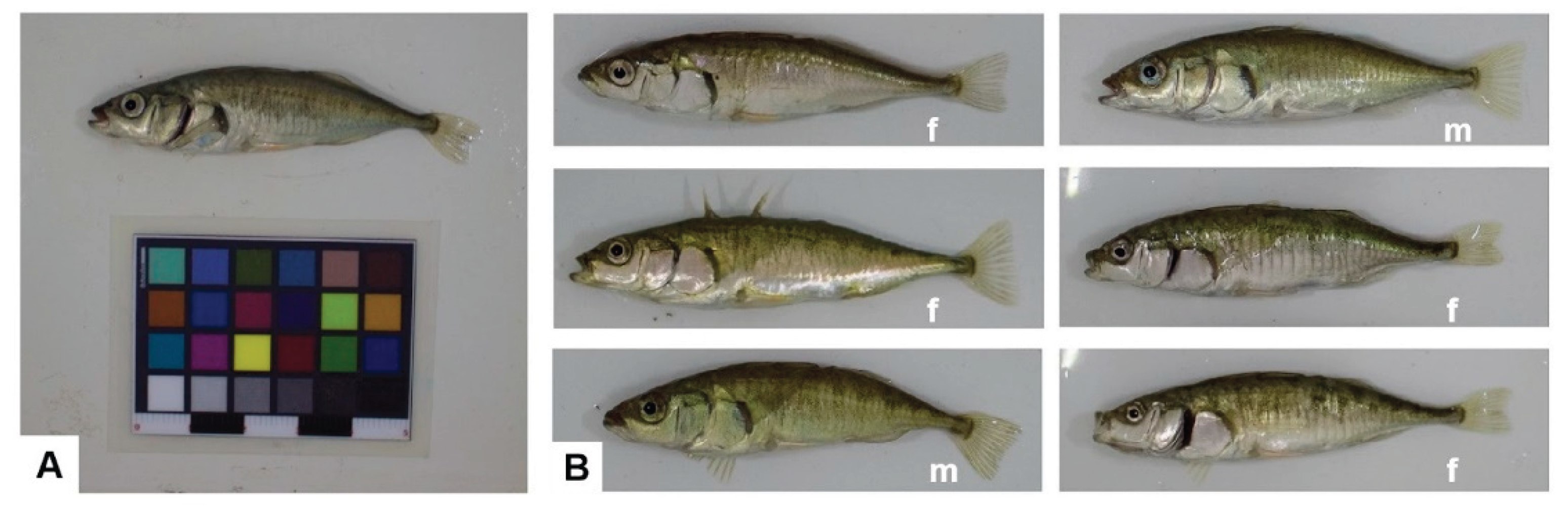
Figure 2.
Distribution of studied standard sites (SS) of threespine stickleback coloration in the White Sea. Each site is sized at 20x20 pixels, consistent with the original image resolution of 3456 x 5184 pixels. SS Points: 1 - 2/3 distance from the back to the line B; 2 – the midpoint on the line A between its intersection with lines B and C; 3 – just above the midpoint between the edges of lines B (urogenital aperture) and C on the ventral side; 4 - the midpoint on the line A within the operculum; 5 - the center of the preoperculum on line D; 6 - eye iris (up): a point on the iris above the center of the pupil; 7 - eye iris (right): a point on the iris behind the center of the pupil; 8 - lateral side behind the head: 1/4 (closer to the back) of the line E. Lines: A - the body midline; B – from the base of the 3rd dorsal spine to urogenital aperture; C – from the base of the 3rd dorsal spine to the lower edge of the body; D - lower edge of the eye and the lower border of the preoperculum; E – from the base of the first dorsal spine to the body midline (lines E, D, C are perpendicular to A). (A) Colors on top plate reflect sex-related (red) and cryptic (yellow) coloration; (B) Each site is marked in the unique color on the bottom plate.
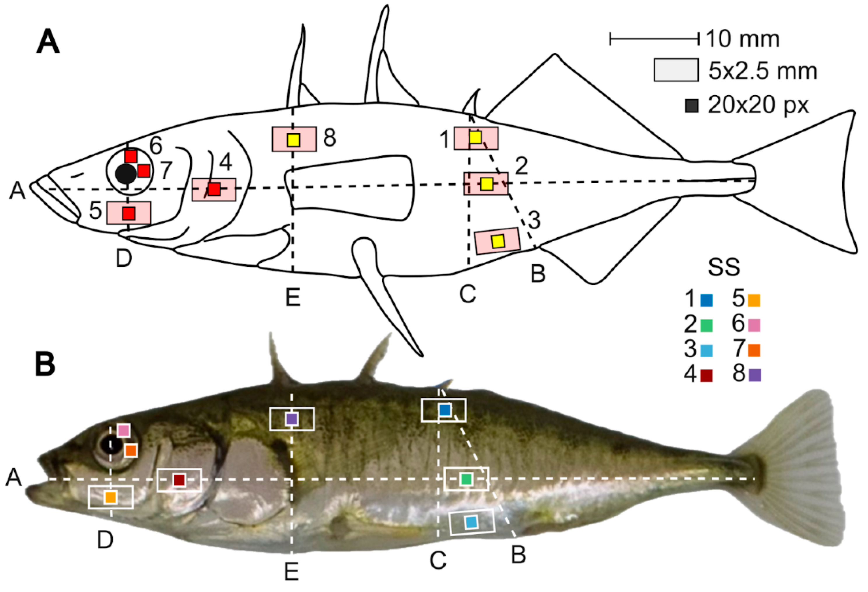
Figure 3.
Raincloud plots of internal variability in CIELAB L* color parameter in experimental and in field data sets. Colors correspond to each SS, violin plots display the underlying distribution of each parameter, boxplots display medians and interquartile range. Colored lines connect mean values indicated as larger points with black contour. Smaller jittered points represent the values of L* in individual fish.
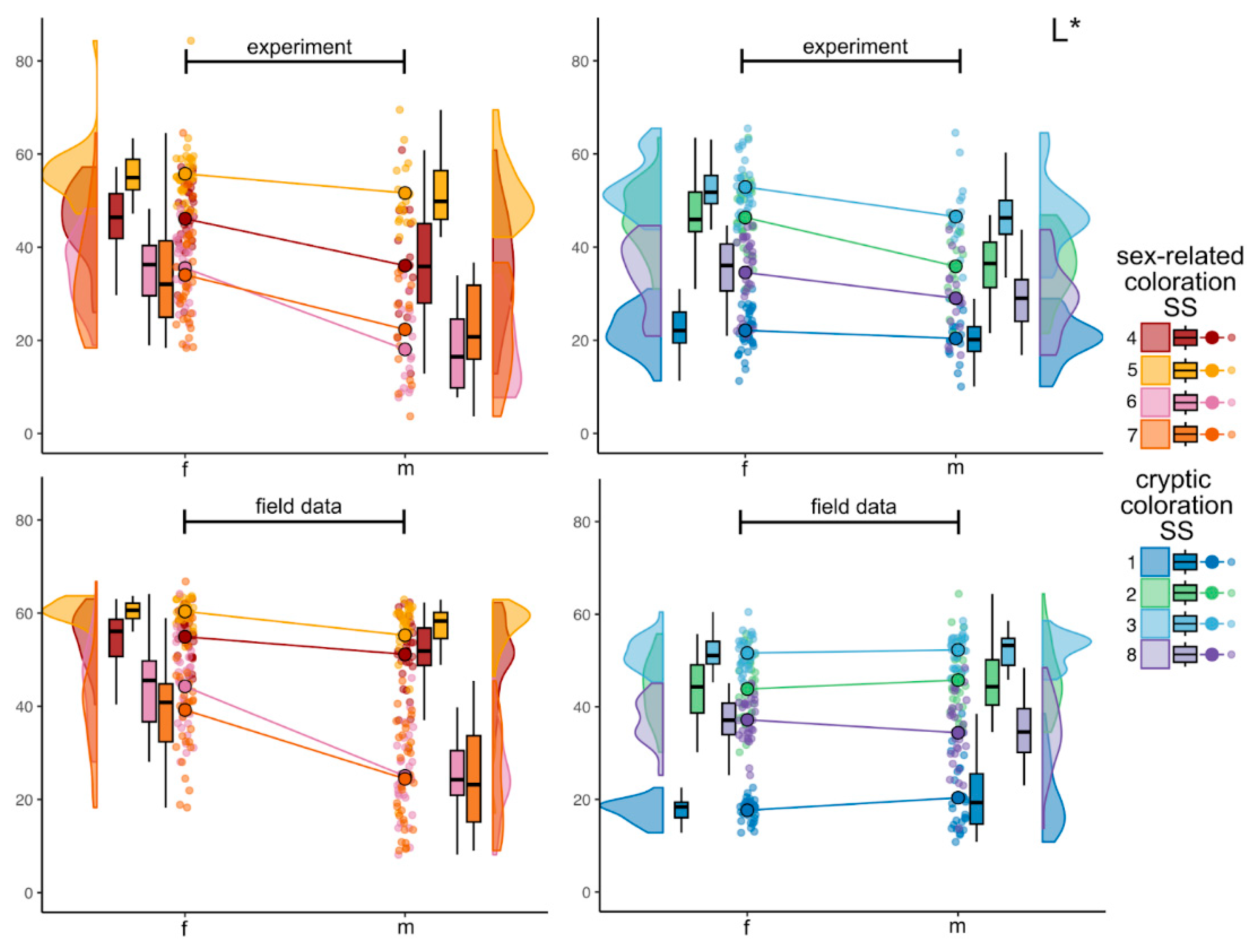
Figure 4.
Raincloud plots of internal variability in CIELAB a* color parameter in experimental and in field data sets. Colors correspond to each SS, violin plots display the underlying distribution of each parameter, boxplots display medians and interquartile range. Colored lines connect mean values indicated as larger points with black contour. Smaller jittered points represent the values of a* in individual fish.
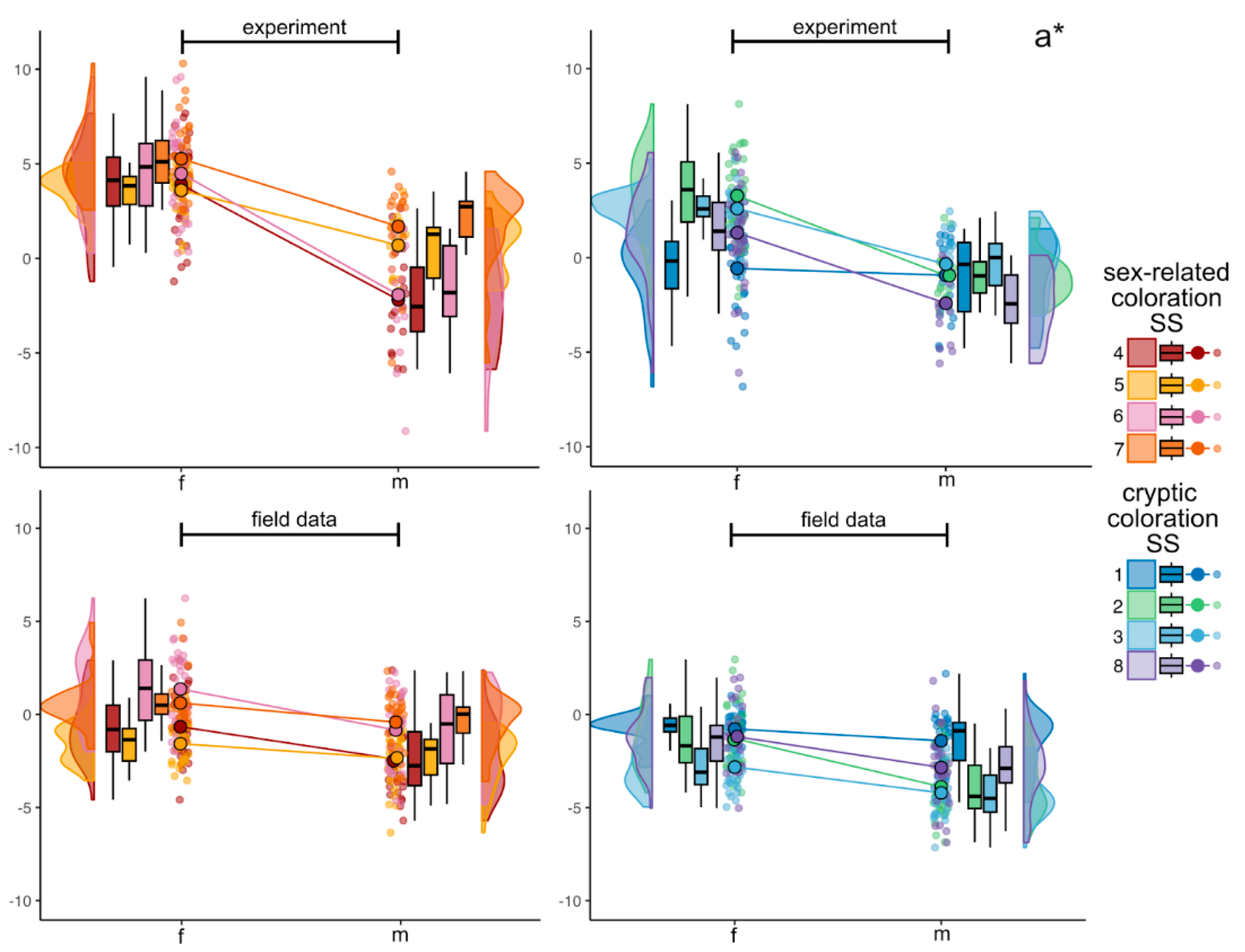
Figure 5.
Raincloud plots of internal variability in CIELAB b* color parameter in experimental and in field data sets. Colors correspond to each SS, violin plots display the underlying distribution of each parameter, boxplots display medians and interquartile range. Colored lines connect mean values indicated as larger points with black contour. Smaller jittered points represent the values of b* in individual fish.
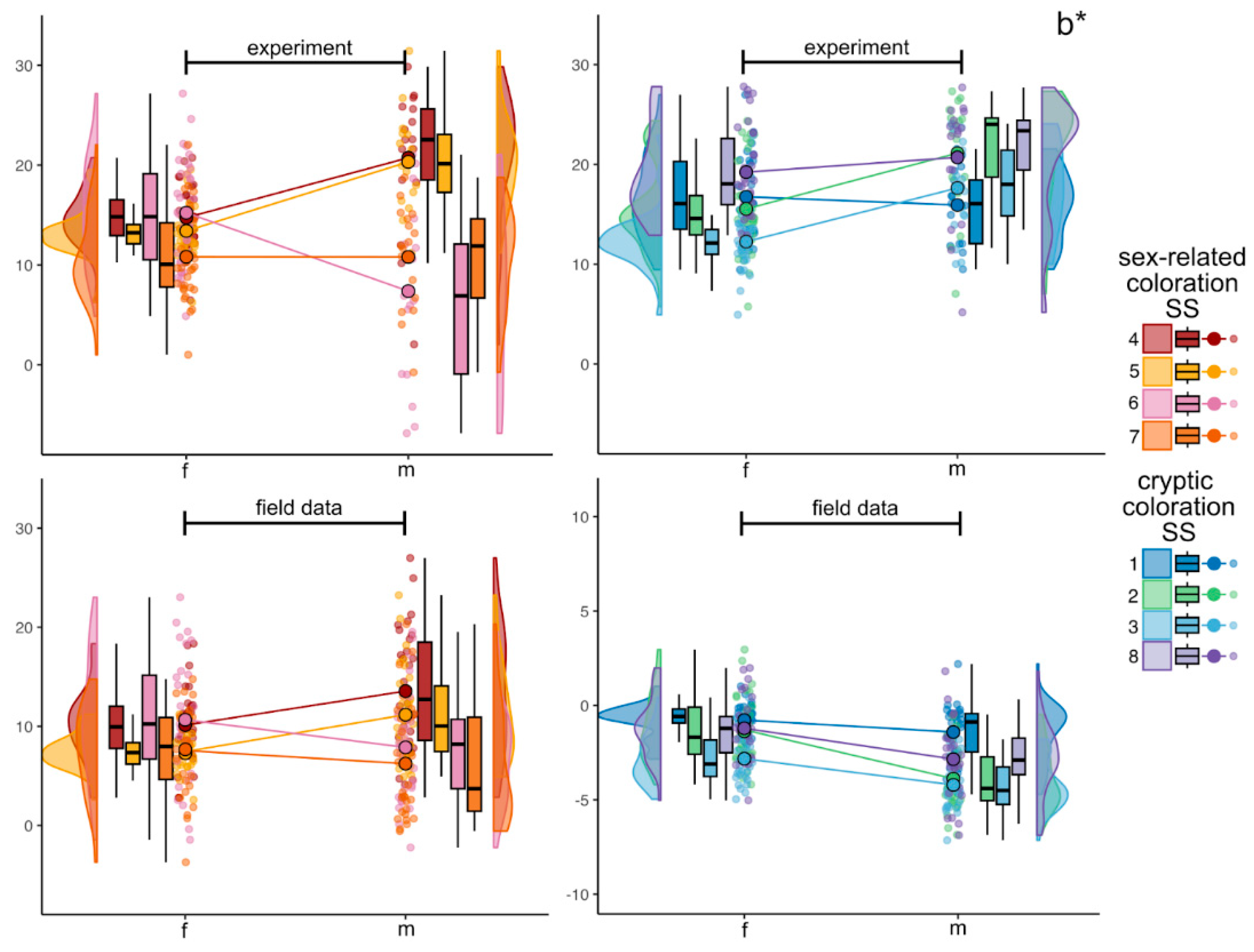
Figure 6.
Mean values, standard deviations and individual values of CIE-L*a*b* color parameters of studied standard sites (SS) across various parts of threespine stickleback body obtained in pool experiment and using field data. Gradient-filled stripes represent color change associated with each color parameter. Asterisks placed by the lines connecting means indicate significant (p<0.05) differences between coloration of SS in males and females according to the Student t-test or Mann-Whitney U test depending on the normality of distribution of variables. For details see Table S1A and Table S1B.
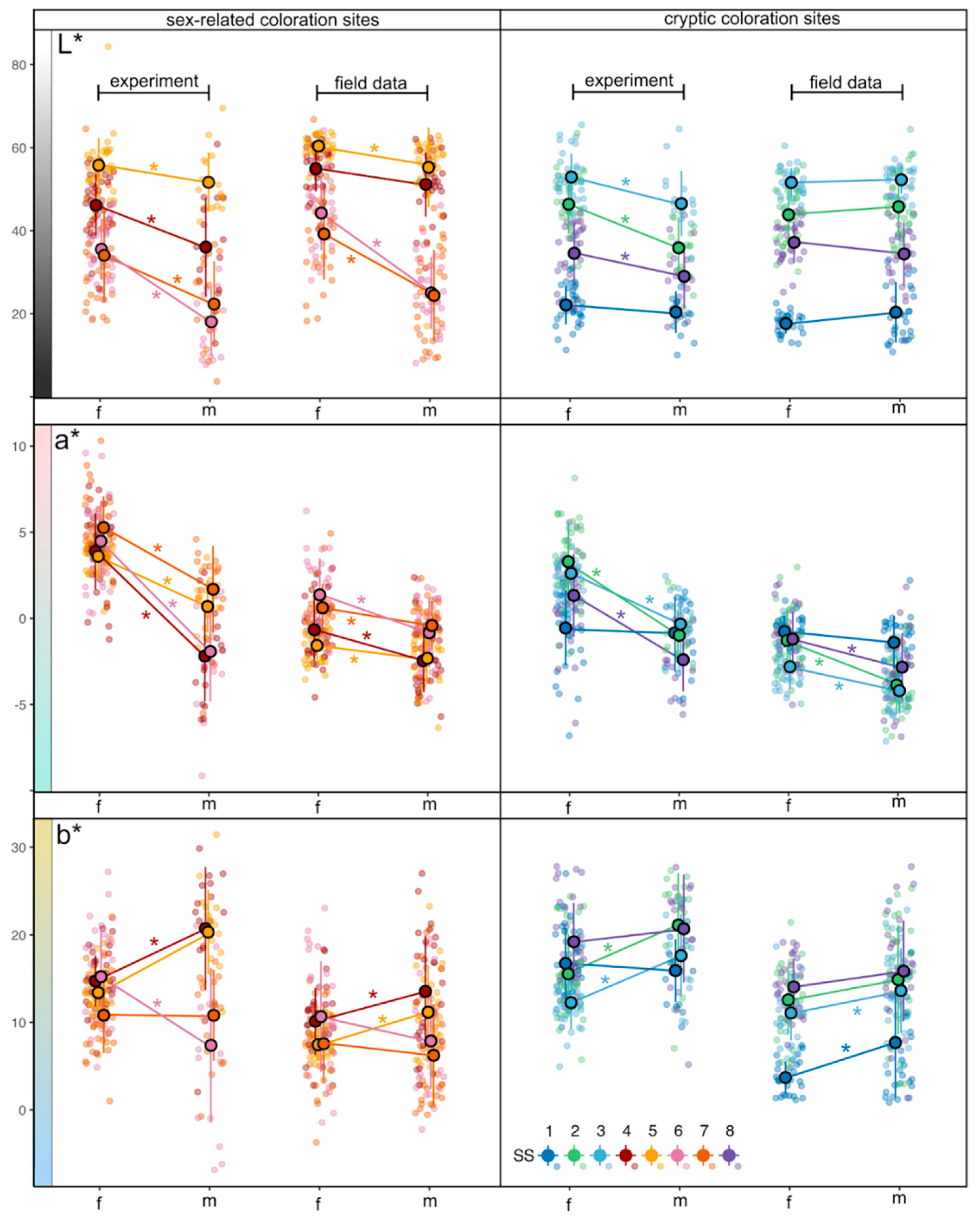
Figure 7.
Results of Principal Component Analysis of standardized CIELAB color data of threespine stickleback coloration based on eight standard sites (SS) in the space of components 1 and 2. Males and females dots are colored in orange and blue respectively. Loadings of 24 variables included 3 parameters (L*, a* and b*) for eight SS also shown on the graph. Ellipses demonstrate 95% confidence intervals. Loadings colors correspond with the colors for SS1-8 at Figure 2, Figure 3, Figure 4, Figure 5 and Figure 6. Red crosses demonstrate mean points within each convex hull.
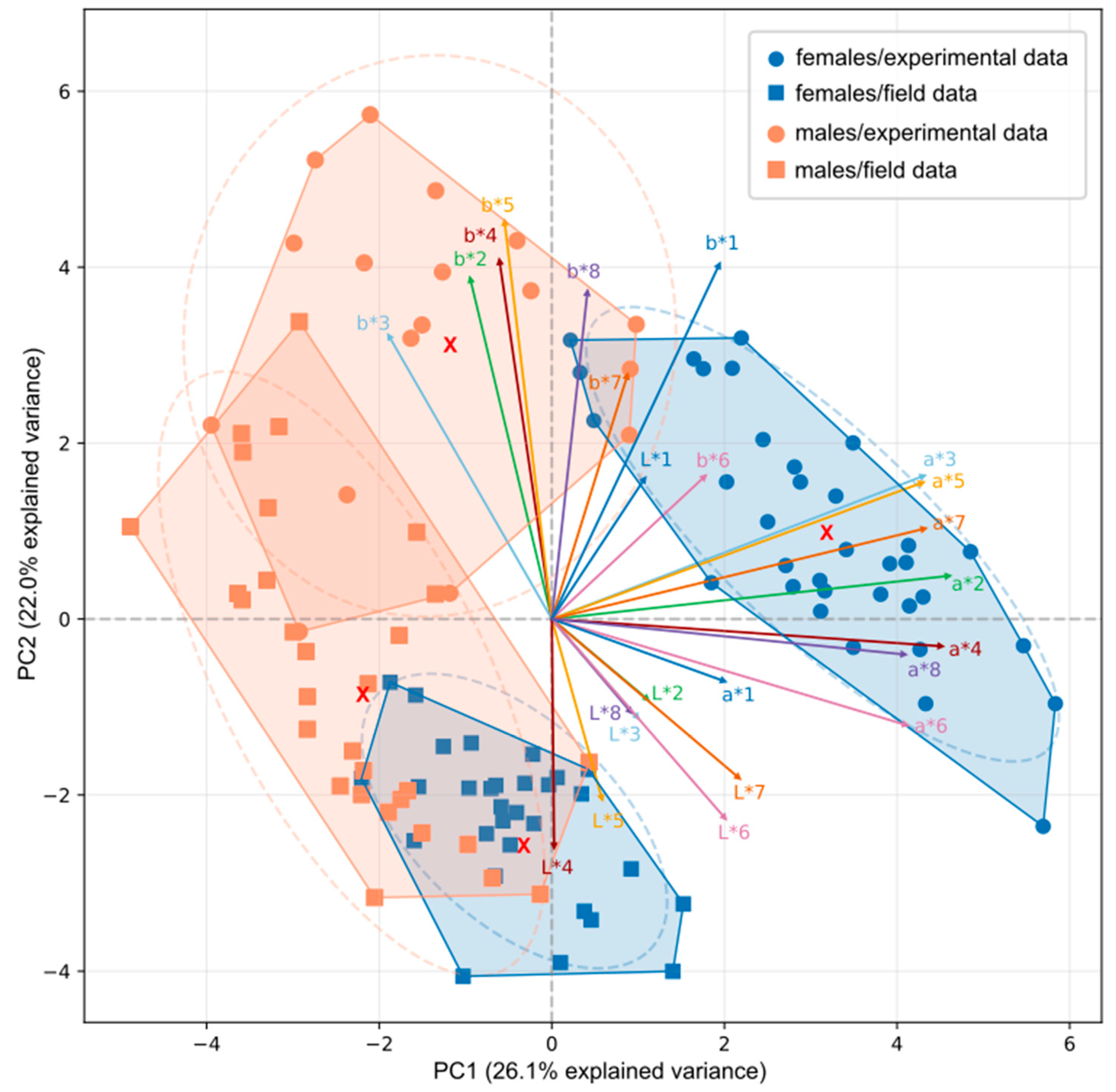

Table 1.
Pigmentation index (∆E*) comparisons between sexes within and between experimental and field datasets. Mean±SD are in the numerator; minimum and maximum values are in the denominator. For experiment data calculations a 34x17 comparison matrix was used, and for field data a 30x30 comparison matrix was used.
| SS | Comparisons | ||||||
|---|---|---|---|---|---|---|---|
| Females vs males, experiment | Females vs males, field | Experiment vs field, females | Experiment vs field, males | ||||
| 1 | 6.17±2.77 | 6.54±5.39 | 10.30±3.05 | 9.54±3.28 | |||
| (0.81-17.75) | (0.24-23.51) | (3.35-20.40) | (1.64-21.43) | ||||
| 2 | 13.72±6.54 | 8.99±3.81 | 11.33±4.49 | 13.12±6.55 | |||
| (0.87-38.58) | (0.43-23.64) | (1.11-33.19) | (1.89-41.06) | ||||
| 3 | 11.34±5.64 | 6.15±2.96 | 9.71±3.00 | 11.15±4.27 | |||
| (1.69-32.29) | (0.43-16.09) | (2.74-21.73) | (3.34-25.90) | ||||
| 4 | 14.66±4.49 | 9.00±4.13 | 13.19±5.93 | 17.94±8.31 | |||
| (2.15-26.12) | (0.56-23.43) | (2.69-35.39) | (2.31-44.77) | ||||
| 5 | 9.70±4.33 | 6.81±4.80 | 10.66±3.10 | 12.64±5.59 | |||
| (1.20-30.59) | (0.55-23.74) | (4.45-26.49) | (1.55-49.06) | ||||
| 6 | 17.00±5.96 | 14.81±6.19 | 13.85±6.51 | 11.91±5.58 | |||
| (1.60-31.21) | (1l.68-37.35) | (1.46-41.84) | (1.01-33.43) | ||||
| 7 | 12.12±6.55 | 12.47±6.73 | 14.64±7.28 | 12.15±5.30 | |||
| (1.39-37.82) | (0.22-35.37) | (3.04-44.43) | (1.61-31.25) | ||||
| 8 | 10.67±3.99 | 7.89±3.86 | 8.94±3.43 | 10.23±4.85 | |||
| (1.45-23.03) | (0.69-21.73) | (1.03-19.83) | (0.64-27.50) | ||||
Disclaimer/Publisher’s Note: The statements, opinions and data contained in all publications are solely those of the individual author(s) and contributor(s) and not of MDPI and/or the editor(s). MDPI and/or the editor(s) disclaim responsibility for any injury to people or property resulting from any ideas, methods, instructions or products referred to in the content. |
© 2025 by the authors. Licensee MDPI, Basel, Switzerland. This article is an open access article distributed under the terms and conditions of the Creative Commons Attribution (CC BY) license (http://creativecommons.org/licenses/by/4.0/).
Copyright: This open access article is published under a Creative Commons CC BY 4.0 license, which permit the free download, distribution, and reuse, provided that the author and preprint are cited in any reuse.


