Submitted:
27 May 2025
Posted:
28 May 2025
You are already at the latest version
Abstract
The occurrence of corporate defaults has manifested as a significant issue for financial entities and stakeholders. Within an increasingly complex economic environment, there is a pressing need to develop innovative approaches for accurate financial risk assessment. One promising approach to preempt crises—particularly bankruptcies—is leveraging insights from other distressed or bankrupt firms. This necessitates the systematic collection and rigorous analysis of corporate financial data. However, such data presents a significant processing challenge: class imbalance. Imbalanced datasets are characterized by a disproportionate distribution of samples across classes. In practice, this means that the information available for one class (typically the bankrupt class) is insufficient—its observations are vastly outnumbered by those of the majority class (non-bankrupt firms). Crucially, the minority class is often the primary focus of interest. The scarcity of samples for this class would be less problematic if conventional classification techniques, such as Support Vector Machines (SVMs), did not inherently bias their predictions toward the majority class due to their generalization tendencies. It is imperative to acknowledge that the intricate arrangement of data significantly intensifies the issue at hand. Not only does data scarcity in the minority class impair machine learning performance, but the intrinsic complexity of the data (e.g., overlapping features, nonlinear separability) can also degrade model accuracy. These twin challenges—class imbalance and data complexity—are key obstacles in bankruptcy prediction. To address these issues, this paper employs Granular Computing techniques, including fuzzy sets, rough sets, shadowed sets, and Quotient Space Theory which offer a robust framework for modeling the nuanced membership functions relevant to the minority class (bankrupt firms). We further propose a hybridization of these techniques to optimize performance. Empirical validation conducted on practical datasets demonstrates that our Fuzzy Shadowed Support Vector Machine (Fuzzy Shadowed SVM) significantly outperforms traditional machine learning methodologies, achieving enhanced predictive accuracy.
Keywords:
Support Vector Machine
; Machine Learning
; Supervised Learning
; Granular Computing
; Imbalanced Data
; Fuzzy sets
; Rough sets
; Shadowed sets
; Quotient Space Theory
; Banckruptcy Prediction
1. Introduction
Corporate bankruptcy represents a critical event with profound economic and social repercussions. This phenomenon impacts not only business owners and employees but also commercial partners, investors, and the broader financial ecosystem [11]. In the contemporary economic landscape characterized by heightened volatility, unpredictability, and competition, the capacity to foresee corporate financial turmoil has emerged as a crucial strategic necessity. Early detection of warning signals enables stakeholders to implement proactive risk mitigation measures, reallocate resources, and potentially prevent economic collapse [22]. This pressing need has driven growing interest in developing sophisticated bankruptcy prediction models that combine analytical rigor with computational power [1]. Traditional bankruptcy prediction studies relied on classical statistical methods such as linear discriminant analysis, logistic regression, and financial scoring models like Altman’s (1968) Z-score [12]. Although these methodologies have substantially enhanced our comprehension of failure mechanisms, they also exhibit numerous constraints. Most notably, their capacity to capture complex nonlinear relationships between explanatory variables and bankruptcy probability is constrained. Furthermore, they typically impose strict assumptions about data normality and variable independence that are rarely satisfied in real-world financial data [31].
The advent of machine learning (ML) methodologies has proffered optimistic solutions to surmount these constraints. ML offers more flexible, adaptive, and powerful tools for modeling the inherent complexity of economic phenomena [2]. Unlike statistical approaches, ML algorithms impose no a priori functional form on variable relationships, enabling them to capture complex interactions and nonlinear effects prevalent in financial data [26]. Popular methods in this domain include Random Forests, Support Vector Machines (SVMs), and ensemble techniques like gradient boosting (XGBoost, LightGBM, CatBoost) [36] ML’s advantages for bankruptcy prediction include its ability to [8]
- Process heterogeneous datasets
- Handle missing or noisy variables
- Adapt to high-dimensional data structures
- Learn from vast historical observation sets to generate robust predictions
However, these approaches also present challenges:
- Significant data preprocessing requirements
- Reduced interpretability compared to traditional models
- Performance sensitivity to hyperparameter selection
- Computational complexity in some implementations
In light of the proliferation of extensive datasets and refined computational technologies, deep learning (DL) strategies have garnered considerable attention in the area of financial forecasting. As a subset of ML, DL employs deep neural architectures capable of automatically extracting hierarchical representations from raw data. Artificial Neural Networks (ANNs), Convolutional Neural Networks (CNNs), Recurrent Neural Networks (RNNs), and specialized variants like Long Short-Term Memory (LSTM) networks have demonstrated effectiveness across diverse applications, including financial and economic forecasting [35]. In bankruptcy prediction, DL architectures achieve high performance by [2]
- Precisely modeling temporal sequences in financial data
- Capturing complex nonlinear interactions
- Leveraging massive datasets for improved generalization
- LSTM networks are particularly well-suited for financial time series analysis due to their ability to capture long-term dependencies
- CNNs have proven effective for extracting discriminative features from transformed financial ratio matrices or tabular representations
Despite their predictive power, DL techniques face criticism regarding:
- High computational complexity and resource requirements
- "Black box" nature that reduces interpretability
- Difficulty justifying predictions for critical applications like credit assessment
Model performance fundamentally relies on data quality. The availability, accuracy, frequency, and granularity of financial information significantly impact predictive system effectiveness. Traditional accounting data, while informative, may insufficiently capture a company’s true financial health dynamics. Emerging research explores integrating alternative data sources (e.g., annual reports, economic news, social media signals) to enrich model training.
A critical additional challenge is class imbalance - a common issue in bankruptcy datasets where non-bankrupt firms vastly outnumber bankrupt ones. Technically, a dataset is considered imbalanced when there exists significant (or extreme) disproportion between class representations. Standard ML algorithms typically exhibit bias toward the majority class because [4]: Rules correctly predicting majority instances receive positive weighting in accuracy metrics
Minority class prediction rules may be treated as noise
Minority instances are consequently misclassified more frequently
The principal contributions delineated within this article may be encapsulated as follows:
- We propose a comprehensive framework of the Fuzzy Support Vector Machine (Fuzzy SVM) using a diverse range of membership functions, including geometric, density-based, and entropy-driven approaches, to quantify the uncertainty of individual samples and enhance model robustness in imbalanced data scenarios.
- We extend the Rough Support Vector Machine (Rough SVM) paradigm by integrating multiple weighting strategies that reflect the granularity of lower and upper approximations, enabling the model to better capture data ambiguity and improve classification performance.
- We introduce a novel Shadowed Support Vector Machine (Shadowed SVM) approach that employs a Multi-Metric Fusion mechanism to define shadow regions near the decision boundary. This is achieved through a combination of geometric distances and margin-based metrics, followed by shadowed combination to control the influence of uncertain instances.
- We develop a Quotient Space Support Vector Machine (QS SVM) model that utilizes a Quotient Space Generator per class. This mechanism delineates the input space into localized regions by employing clustering algorithms, including K-Means or DBSCAN, thus facilitating the model’s ability to develop classifiers that are specific to each region and to accommodate the variations inherent in local data distributions.
- We empirically observe that Fuzzy SVM excels in achieving high overall accuracy, while the Shadowed SVM provides superior performance in handling data imbalance. Motivated by these complementary strengths, we propose a novel hybrid model—Fuzzy Shadowed Support Vector Machine (Fuzzy Shadowed SVM)—which combines fuzzy membership weighting with shadowed instance discounting to achieve both high accuracy and class balance.
The subsequent sections of this manuscript are organized as delineated below: Section 2 offers an extensive examination of the existing literature pertinent to the prediction of bankruptcy. Section 3 discusses the concept of granular computing, particularly fuzzy sets, rough sets, shadowed sets, and quotient space theory. Section 4 offers a concise overview of the proposed granular Support Vector Machine approach . Section 5 delineates the empirical findings and their subsequent examination, whereas Section 7 articulates the ramifications of the results, delineates prospective avenues for further investigation, and encapsulates the principal contributions and outcomes of this scholarly endeavor.
2. Literature Review
Corporate bankruptcy prediction has long represented a critical challenge in quantitative finance and risk management. Identifying early warning signals enables financial loss anticipation, credit risk assessment, investment optimization, and economic policy guidance. As available data grows in volume and variety, traditional methods face inherent limitations, while machine learning (ML)[23] and deep learning (DL) [35] techniques emerge as powerful adaptive alternatives.
However, applying these techniques to bankruptcy prediction encounters a persistent structural obstacle: class imbalance in datasets. Bankrupt firms typically constitute a tiny minority (often <5%, sometimes <1%) in real-world databases. This disparity between the majority class (solvent firms) and minority class (bankrupt firms) fundamentally challenges effective predictive model development [6].
Early bankruptcy prediction research was dominated by statistical models like linear discriminant analysis (Altman 1968), logistic regression (Ohlson 1980), and financial scoring models (Z-score, O-score) [29]. While robust, these exhibit critical limitations with imbalanced data: their parametric nature imposes strict distributional assumptions (normality, variable independence) rarely satisfied empirically, and their symmetric cost functions minimize overall error without distinguishing minority-class misclassification impacts - precisely the class of interest.
Consequently, while such models achieve high accuracy rates, they frequently demonstrate poor sensitivity (recall) for bankrupt firms, yielding excessive false negatives - a critical error in risk management contexts. For instance, in datasets with only 3% bankrupt firms, a trivial "always solvent" classifier achieves 97% accuracy while failing completely at bankruptcy detection.
To address this imbalance, researchers initially explored data-level rebalancing techniques before model training, primarily:
- Oversampling: Artificially augmenting the minority class via random duplication (Random Oversampling) or synthetic generation (e.g., SMOTE [19]), which interpolates new instances from real examples.
- Undersampling: Reducing the majority class via random subset selection, though risking information loss about healthy firms.
- Advanced hybrids (Borderline-SMOTE, ADASYN, SMOTEENN) [28] combine these approaches. Empirical studies demonstrate these techniques significantly improve minority-class metrics like recall, weighted precision, and AUC-ROC (Zhou et al. 2019; Martín-Jiménez 2020).
Machine learning algorithms have attained extensive utilization in contemporary bankruptcy research owing to their ability to elucidate nonlinear interdependencies, manage diverse data types, and enhance the generalizability of predictive models. Prominent approaches include( [26,27]
- Random Forests: Bootstrap-aggregated decision trees robust to noise and correlations
- Support Vector Machines (SVM): Margin-maximizing classifiers in transformed spaces
- Decision Trees (CART, C4.5): Interpretable rule-based models
- Boosting algorithms (XGBoost, LightGBM, CatBoost): Ensemble methods combining weak learners
To counter class dominance effects, key strategies include:
- Cost-sensitive learning: Algorithms like XGBoost permit class weighting (scale pos-weight) to penalize minority-class errors
- Integrated sampling: Techniques like Balanced Random Forest perform per-iteration resampling
- Alternative metrics: F1-score, AUC-PR, G-mean, or Matthews Correlation Coefficient (MCC) better evaluate imbalanced contexts [37].
Empirical studies confirm these approaches, combined with judicious data rebalancing, improve overall performance while maintaining bankruptcy detection capability ( [10,33]).
DL methods have rapidly expanded in financial applications due to automated feature extraction capabilities. Research has shown that Convolutional Neural Networks (CNNs) [9] work effectively for predicting bankruptcies [16]. These methodologies also demonstrate considerable efficacy when integrated with alternative techniques, including Recurrent Neural Networks (RNNs/LSTMs) [17] and diverse configurations of Artificial Neural Networks (ANNs) [14].
However, with severe class imbalance, these models become prone to majority-class overfitting, particularly when bankruptcies are extremely underrepresented. Additionally, their massive data requirements complicate application in low-default portfolios. Mitigation strategies include:
- Weighted loss functions: Modifying binary cross-entropy with class-frequency weights or adopting focal loss [30] to emphasize hard samples
- Balanced batch training: Curating mini-batches with controlled class proportions [20]
- Temporal data augmentation: For LSTM/GRU models, generating synthetic sequences via dynamic time warping or Gaussian perturbation [18]
A critical adoption barrier for complex models - especially in finance - remains interpretability. Deep neural networks often function as "black boxes", providing accurate predictions without decision transparency. Post-hoc explanation tools like LIME [21] and SHAP [34] address this by quantifying variable importance for individual predictions, even on rare cases. Alternative approaches embed interpretability directly into model architectures through neural-rule hybrids or accounting-informed filtering layers. Toward Hybrid and Multimodal Approaches:
- Data-level rebalancing (SMOTE, ADASYN)
- DL representation power
- Secondary classifiers (e.g., Random Forest, XGBoost) for refined decisions
Innovations include incorporating textual data (financial reports, news) via NLP models and behavioral indicators. Here’s a more humanized version of your text:
For example, Zhang et al. [32] integrate an autoencoder to detect anomalies in financial ratios, an LSTM network for capturing sequential patterns, and SHAP explanations to support human interpretation. Building on this, Wang and colleagues [25] show that using CNN-LSTM models trained on SMOTE-generated synthetic data can substantially improve prediction accuracy, boosting both F1-scores and recall rates.
ML/DL-based bankruptcy prediction constitutes a rapidly evolving field constrained by inherent class imbalance. This structural data characteristic biases conventional models, necessitating specialized data treatments and algorithmic adaptations. While oversampling, cost-sensitive learning, weighted loss functions, and hybrid approaches demonstrate effectiveness, the field must still reconcile predictive performance with stability, generalizability, and interpretability - particularly in regulated finance, banking, and auditing contexts.
3. Granular Computing
Granular computing elucidates the manner in which granular reasoning may be utilized to forecast corporate insolvency. For instance, artificial neural networks—with fuzzy concept such as those referenced by Jabeur et al. [40] are used to sort and classify a wide range of economic data while accounting for the diverse behaviors of various economic agents. A well-orchestrated training process enables these models to uncover, sometimes in unexpected ways, hidden structures within highly complex datasets, thereby making it easier to detect early warning signals of financial distress. Borowska et al. [15] have advocated for an updated version of the rough–granular approach (RGA), aiming to improve the classification performance on bankruptcy data. Granular computing focuses on multi-level data processing—an emerging domain that already shows significant promise. It involves organizing information in a hierarchical manner, which proves particularly useful for analyzing complex systems such as corporate bankruptcy prediction. Typically, the use of multiple datasets enriches predictive models.
In the long term, the goal is to improve decision-making processes and risk assessment strategies within the financial sector. By developing more accurate predictive models, stakeholders can better identify at-risk firms, enabling timely interventions and fostering a more resilient financial environment.
Support Vector Machine (SVM) has emerged as a preeminent classification methodology in the domain of bankruptcy prediction, attributable to its robust theoretical underpinnings and its capacity to delineate an optimal hyperplane that maximizes the separation between distinct classes. Its efficacy is especially pronounced in high-dimensional parameter spaces, wherein SVM adeptly differentiates between solvent and bankrupt enterprises by employing kernel functions that elucidate non-linear relationships within financial metrics. Furthermore, SVM demonstrates commendable generalization capabilities even when confronted with sparse training datasets, a phenomenon frequently encountered in financial analytics. Nevertheless, notwithstanding its advantages, SVM is confronted with a substantial limitation when deployed in the context of imbalanced datasets, a prevalent feature of bankruptcy forecasting wherein non-bankrupt entities vastly outnumber their bankrupt counterparts. In such instances, the conventional SVM exhibits a propensity to favor the majority class, resulting in inadequate identification of the minority class (i.e., bankrupt firms). This bias arises from the margin-based optimization paradigm, which fails to explicitly account for class distribution. Consequently, the classifier may attain a high overall accuracy yet inadequately recognize instances of financial distress, thereby undermining its practical applicability in the realm of real-world bankruptcy prediction.
To address the challenges posed by imbalanced datasets in bankruptcy prediction, numerous techniques grounded in Granular Computing (GrC) have been proposed. Granular computing provides a powerful paradigm for processing complex and uncertain information by decomposing data into meaningful granules. In this context, several researchers have explored granular-based strategies to enhance data representation and learning performance. Among these, the work of Shuyin Xia et al. [3] introduced the concept of granular-ball computing within the framework of fuzzy sets, aiming to improve the preprocessing phase of imbalanced classification. The authors proposed a novel fuzzy set model where the data space is adaptively covered using a set of hyperspheres (granular-balls), each representing a localized region of the input space. These hyperspheres are generated based on the distribution of the data, and the boundary points of the balls serve as representative sampled data. This approach effectively reduces data redundancy while preserving critical structural information, thereby enhancing the learning process in fuzzy environments. The granular-ball model offers a promising direction for mitigating the impact of class imbalance by enabling more balanced data distribution through adaptive sampling and localized granulation.
In conjunction with granular-ball computing, numerous alternative granular computing paradigms have been formulated to mitigate data imbalance through the alteration of either the data distribution or the intrinsic learning mechanism. Granular Support Vector Machines (GSVM) represent a notable example, where the input space is divided into granular regions, each associated with specific levels of uncertainty or importance. This decomposition facilitates the design of more robust classifiers by emphasizing the minority class during training, thus improving sensitivity and generalization.
Moreover, granular computing has been effectively amalgamated with additional soft computing frameworks, including rough sets and fuzzy sets [5,13,24,38,39]. For instance, hybrid models that combine fuzzy set theory with granular principles enable the construction of fuzzy partitions that are sensitive to local imbalances. These partitions can adaptively reflect the underlying data distribution, which is especially critical in domains such as bankruptcy prediction, where misclassifying a minority instance can have significant financial implications A representative approach in this direction is the work of Ibrahim, H et al. [13], who proposed a Rough Granular SVM (RG-SVM) that incorporates rough approximations into the granular structure of the input space. The model leverages lower and upper approximations to deal with boundary uncertainty, allowing the classifier to differentiate more effectively between borderline and well-defined instances. This technique not only improves classification accuracy but also enhances the interpretability of the decision regions.
3.1. Fuzzy Sets
The fuzzy set methodology, initially proposed by Lotfi A. Zadeh in the year 1965, constitutes a pivotal extension of traditional set theory. It enables the modeling of vagueness and uncertainty intrinsic to many complex systems, including engineering, artificial intelligence, economics, and social sciences.
In traditional set theory (often called crisp sets), membership is black and white - an element either fully belongs to a set or doesn’t belong at all, with no middle ground. In other words, for any element x in the universe U, the membership function of a set A takes values exclusively in {0, 1}:
This binary framework demonstrates efficacy for distinctly defined parameters (e.g., “Is it an even integer?”, “Is he/she a citizen of the state?”); however, it is insufficient for the representation of ambiguous or continuous constructs such as “tallness,” “youthfulness,” “riskiness,” or “low socioeconomic status.”
Fuzzy set theory offers a more flexible framework that corresponds with the elusive nature of human communication and the complexities of the empirical realm. A fuzzy set over a universe X is defined by a membership function , which assigns to each element a membership degree ranging from 0 to 1.
For example, in a fuzzy set , one might have:
This implies that 1.80 m is somewhat tall, 1.90 m is very tall, and 2.00 m is fully tall.
Key characteristics of fuzzy sets include:
- Membership Function: The core of fuzzy logic, which can take various shapes (triangular, trapezoidal, Gaussian, sigmoidal), chosen according to interpretative or modeling needs.
- Support: The set of elements where , indicating the domain of influence.
- Core: The set of elements where , representing full membership.
- Height: The maximum value of ; the set is normalized if the height equals 1.
Fuzzy operations generalize classical set operations:
- Union:
- Intersection:
- Complement:
Advanced operators such as t-norms and t-conorms allow for more refined conjunctions and disjunctions.
The utility of fuzzy sets lies in their ability to incorporate approximate reasoning into computational systems. For example, in an intelligent driving system, rules like:
“If speed is high and visibility is low, then decelerate sharply”
are based on subjective concepts that fuzzy sets represent effectively.
Applications encompass:
- Fuzzy control mechanisms (e.g., thermal regulation, self-operating vehicles)
- Multi-criteria decision analysis under conditions of uncertainty (fuzzy Analytic Hierarchy Process, fuzzy Technique for Order of Preference by Similarity to Ideal Solution)
- Medical diagnostics involving indistinct symptoms
- Fuzzy data examination and clustering methodologies (e.g., fuzzy c-means algorithm)
- Risk assessment and behavioral finance considerations
- Expert systems and symbolic artificial intelligence
Despite their advantages, fuzzy sets have limitations:
- Subjectivity in choosing membership functions
- Difficulty in aggregating a large number of fuzzy rules
- Increasing computational complexity in large-scale systems
- Unsuitability for random uncertainties (where probability theory is more appropriate)
Extensions encompass:
- Type-2 Fuzzy Sets (characterized by uncertainty pertaining to the membership function itself)
- Intuitionistic Fuzzy Sets (which incorporate a quantifiable measure of non-membership)
- Rough Sets (which are pertinent within contexts reliant on granularity)
Fuzzy set theory represents a significant conceptual evolution in the representation of imprecise phenomena. By diverging from rigid binary logic, it facilitates the development of models that more accurately reflect human cognitive processes, exhibit enhanced flexibility, and are better aligned with the ambiguity that characterizes real-world scenarios. Its incorporation into hybrid frameworks (neuro-fuzzy systems, fuzzy expert systems, extended fuzzy logics) perpetually expands its relevance across the domains of artificial intelligence, engineering, economics, and beyond.
3.2. Rough Sets
The conceptual framework of rough set theory, pioneered by Zdzisław Pawlak in 1982, offers a rigorous mathematical structure for the representation of uncertainty, imprecision, and deficiencies in information within data systems. Unlike probability theory or fuzzy sets, rough sets rely on the concept of indiscernibility: when an object’s membership in a set cannot be determined precisely, upper and lower approximations are used to bound the set. In many real-world contexts—such as machine learning, classification, data mining, and knowledge discovery—available data is incomplete or imprecise, preventing a sharp partitioning of objects. Rough set theory enables reasoning based on approximations by leveraging the indiscernibility relation among observed objects.
The foundation of this study is an information system conceptualized as a table representation. , where:
- U is the Universe: a finite set of objects,
- A represents a finite set of Attributes.
Each attribute is a function , where is the value domain of f.
are indiscernible with respect to a subset if they share identical attribute values over C. This induces an equivalence relation:
This equivalence relation partitions U into equivalence classes known as information granules. Given , the lower and upper approximations are defined as:
- Lower approximation : the set of objects that certainly belong to X, i.e., those whose equivalence classes are fully contained within X:
- Upper approximation : the set of objects that possibly belong to X, i.e., those whose equivalence classes intersect with X:
The rough boundary of X is:
It consists of objects for which membership is uncertain. A set is exact if its boundary is empty (); otherwise, it is rough.
The precision of the approximation is measured by:
This ratio, in , quantifies the confidence in the approximation.
Rough set theory also facilitates attribute reduction and dependence analysis:
- A reduct is a minimal subset of attributes preserving the classification power of the full set.
- The core is the intersection of all reducts—attributes that are indispensable.
Applications of rough sets include:
- Feature selection and dimensionality reduction
- Interpretable decision rule generation
- Analysis of incomplete or imprecise data
- Multi-criteria decision analysis
- Bioinformatics, finance (bankruptcy prediction), healthcare (diagnosis)
Rough set theory is frequently integrated with alternative models (such as fuzzy sets and neural networks) to create sophisticated hybrid frameworks. It is especially effective with discrete data; continuous data must usually be discretized. It is sensitive to data quality and may require preprocessing for large datasets due to the computational cost of reduct calculation.
Overall, rough set theory offers a robust framework for modeling indiscernibility-based uncertainty, complementing probabilistic and fuzzy methods—especially when prior knowledge on membership degrees is lacking
3.3. Shadowed Sets
The conceptual framework of shadowed sets, as delineated by Wang et al. (1992), serves to augment the traditional fuzzy set theory initially articulated by Zadeh (1965). It was developed to address specific limitations of fuzzy sets, particularly the interpretability of membership degrees close to 0.5. Shadowed sets simplify fuzzy representations by offering a three-valued approximation: a definite inclusion, a definite exclusion, and an indeterminate or shadowed region, which captures uncertainty or vagueness In fuzzy modeling, each element x in a universe X is associated with a membership degree . Nevertheless, membership values that approach the median (e.g., ) may present challenges in the interpretation within the framework of decision-making processes. For instance, if , should the element be considered a member of the set or not? This ambiguity can hinder effective decisions in expert systems, classification tasks, or reasoning under uncertainty To overcome this issue, shadowed sets replace the continuum of fuzzy membership values with a three-level approximation:
- ⇒ the element clearly belongs to the set;
- ⇒ the element clearly does not belong to the set;
- ⇒ the element lies in a shadowed region, indicating indeterminacy.
Let A be a fuzzy set over X with membership function . The corresponding shadowed set is constructed using two thresholds and , where . The universe is then partitioned into three distinct regions:
- Positive region (membership 1): if , then ;
- Negative region (membership 0): if , then ;
- Shadowed region (indeterminate): if , then is undefined or remains within .
Illustrative example in fuzzy classification:
- Patient A: ⇒ classified as ill;
- Patient B: ⇒ classified as healthy;
- Patient C: ⇒ classification is indeterminate.
Assuming and , the interpretation is as follows:
Optimal threshold determination: Wang proposed an optimization-based approach to determine the ideal values of and by minimizing the total approximation error:
The goal is to find and (with ) that minimize , thereby maximizing the transfer of ambiguity into the shadowed region while retaining interpretive clarity in the crisp regions.
3.4. Quotient Space Theory
Quotient Space Theory (QST), as delineated by Zhang et al. (2004), presents a systematic approach for the representation of human cognition, positing that this cognition is intrinsically situated, ambiguous, and structured in a hierarchical manner. This theoretical framework is grounded in the mathematical concept of quotient space, a construct frequently employed in topology and abstract algebra, to elucidate the granularity and complexity of information representation Let X be a set representing an information space, and let R be an equivalence relation on X. The relation R partitions X into equivalence classes , each representing an information granule The set of all equivalence classes forms the quotient space:
A quotient space is formally defined as a triplet:
where:
- X is the original information space,
- R is an equivalence relation on X,
- f is a function defined on the equivalence classes of R.
QST is founded on two fundamental cognitive principles:
- Cognitive partiality: human perception is inherently local and approximate,
- Local processing: reasoning is performed within subspaces of the global problem.
These principles justify the construction of a hierarchy of successive quotient spaces, each representing a distinct level of abstraction.
QST introduces a hierarchical tree structure:
- the root node represents the global space,
- lower levels denote finer abstractions,
- child nodes refine the representations of their parents.
In machine learning, each class can be interpreted as a quotient space. QST facilitates:
- dimensionality reduction,
- reasoning over aggregated representations,
- robustness against uncertain or noisy data.
Two fundamental stages are involved:
- Construction of a quotient space: selecting relevant attributes and defining R,
- Reasoning and prediction: operating within a simplified space, and refining representations when uncertainty arises.
Imbalanced data is characterized by the underrepresentation of one or more classes, leading to:
- model bias toward the majority class,
- low recall on the minority class,
- limited generalization capabilities.
QST enables:
- intelligent grouping of data samples,
- localized treatment of the minority class,
- adaptive granularity tailored to rarity.
A Support Vector Machine (SVM) delineates distinct classes by optimizing the separation margin that exists between them. In imbalanced contexts, support vectors from the minority class are often insufficient.
The integration procedure encompasses the subsequent stages:
- Pre-granulation employing QST,
- Structured resampling predicated on granule characteristics,
- SVM training utilizing balanced granules,
- Hierarchical prediction facilitated through a QS Tree framework.
QST facilitates a hierarchical and granular depiction of complexity and uncertainty. When amalgamated with SVM in contexts characterized by imbalanced learning, it markedly improves classification efficacy—particularly for minority classes—while maintaining the integrity of the overarching model architecture. In other words, the integration of QST promotes:
- enhances recall for the minority class,
- mitigates tendencies toward overfitting,
- promotes adaptable and localized decision-making.
4. Granular Support Vector Machines: Proposed Approach
Support Vector Machines (SVM) constitute a formidable approach for tackling classification issues; nevertheless, this conceptual paradigm is not devoid of its drawbacks. Each training instance is assumed to belong exclusively to one of the two defined classes. Clearly, within the SVM paradigm, all training instances relevant to a specific class are treated uniformly The technology of Support Vector Machines has garnered increasing attention within the machine learning community (as evidenced by the vast volume of publications dedicated to SVM) Support Vector Machines (SVM) are based on the principle of Structural Risk Minimization (SRM), which aims to balance model complexity and training error in order to improve generalization performance. . In numerous applications, SVMs have demonstrated superior performance compared to classical learning methods and are now regarded as powerful tools for tackling classification problems SVM involves two main stages: first, it maps input data points into a high-dimensional feature space; then, it seeks to identify a separating hyperplane that optimally maximizes the margin between the two classes within this transformed space. The process of maximizing the margin is formulated as a quadratic programming (QP) problem, which can be efficiently solved by addressing its dual form via Lagrange multipliers Without requiring explicit knowledge of the projection function, the SVM skillfully determines the optimal hyperplane using inner product functions in the feature space, known as kernels. The resulting solution can be expressed as a linear combination of a limited subset of input data points, referred to as support vectors SVM-based methodologies are increasingly adopted across a wide range of disciplines. Notwithstanding, in certain applications, it is not feasible to unequivocally categorize all data points into one of the two delineated classifications. Certain instances are critical and require strict classification to ensure proper separation. Conversely, other data points—possibly affected by noise—are less significant, and it would be advantageous for the model to disregard them Formally, an SVM can be defined as follows:
Let S denote a dataset with training instances , where and .
In numerous instances, the endeavor to directly ascertain a hyperplane within the input space is found to be unduly limiting for effective practical application. A potential solution to this constraint involves projecting the input space into a higher-dimensional feature space and then seeking the optimal hyperplane in this modified environment Support Vector Machines, introduced by Vapnik [7], are a supervised learning method rooted in statistical learning theory. Their primary goal is to determine an optimal decision boundary—called the separating hyperplane—that maximizes the margin between different classes. This methodology, founded upon the principles of convex optimization and kernel theory, is characterized by its resilience and capacity for generalization, even within the confines of high-dimensional spaces.
Let a training set be given by , where represents a feature vector and denotes its label. The optimization problem for a linear SVM is formulated as:
where w is the weight vector orthogonal to the hyperplane, and b is the bias. The optimal solution defines the separating hyperplane , with a margin of .
When data are not linearly separable, SVMs employ a kernel function to map the data into a higher-dimensional space where linear separation becomes feasible. Common kernels include:
- Gaussian Radial Basis Function (RBF) Kernel:
- Polynomial Kernel:
For problems involving noise or class overlap, a soft-margin formulation introduces slack variables , leading to the optimization problem:
where C controls the trade-off between margin maximization and tolerance for misclassification SVMs are widely applied in pattern recognition, text classification, and bioinformatics, due to:
- Their resistance to overfitting
- Their flexibility through kernel selection
- Their effectiveness in high-dimensional spaces
Challenges include hyperparameter tuning (e.g., selecting C and the appropriate kernel), and computational complexity when handling large-scale datasets. Variants including multi-class Support Vector Machines (for instance, one-versus-all methodologies) and Support Vector Regression (SVR) enhance the applicability of the Support Vector Machine paradigm to a more extensive array of challenges. The classical Support Vector Machine (SVM) framework lacks an inherent mechanism to handle the varying importance or informativeness of individual training instances. This limitation becomes critical in scenarios where data quality or relevance differs across the dataset. In many classification tasks, certain examples carry greater significance or provide more valuable information than others. Consequently, it is desirable to achieve high accuracy on these key instances while allowing for some misclassification of noisy or less relevant samples.
Put simply, a training instance should not be strictly assigned to a single class. For instance, an example might belong to a class with 90% confidence and have 10% ambiguity, or alternatively, it may show 20% association with one class and 80% non-relevance. Hence, each sample can be attributed a fuzzy membership degree, which quantifies the level of confidence or affiliation of the instance to a class. The complementary degree indicates the irrelevance or insignificance of the sample in the decision process.
Building on this foundation, we propose enhancing the standard Support Vector Machine (SVM) by incorporating fuzzy membership values—resulting in a more flexible Fuzzy Support Vector Machine (FSVM) model.
Bankruptcy prediction is a crucial financial task aimed at forecasting firms likely to encounter financial distress. A significant challenge arises from the class imbalance inherent in such data: bankrupt firms are far fewer than healthy ones. This imbalance biases classical supervised models, including SVM, towards the majority class.
To tackle these complexities, we propose an advanced augmentation of the conventional Support Vector Machine (SVM) paradigm, designated as the Granular Support Vector Machine (GSVM). This methodology amalgamates various granular computing methodologies, encompassing:
- Fuzzy Support Vector Machine (Fuzzy SVM),
- Rough Support Vector Machine (Rough SVM),
- Shadowed Support Vector Machine (Shadowed SVM),
- Quotient Space Support Vector Machine (QS SVM),
- Fuzzy Shadowed Support Vector Machine (Fuzzy Shadowed SVM).
These approaches aim to better capture the uncertainty, ambiguity, imprecision, and cognitive granularity typically present in noisy or incomplete financial datasets.
This work presents the theoretical foundations, implementation details, and application of each approach in the context of bankruptcy prediction.
Specifically, the Fuzzy SVM assigns fuzzy membership values to training points, reflecting their reliability and handling uncertainty or label noise.
In bankruptcy datasets, some firms exhibit intermediate financial indicators, being neither clearly healthy nor definitively risky. FSVM mitigates the influence of such ambiguous instances by assigning lower weights during optimization, thereby:
- Reducing the impact of outliers,
- Emphasizing firms on the brink of bankruptcy,
- Attenuating bias towards the majority class.
Based on Pawlak’s Rough Set Theory, Rough SVM decomposes the set of companies into three regions:
- The positive region (certainly bankrupt or non-bankrupt),
- The negative region (certainly not bankrupt or bankrupt),
- The boundary region (uncertain).
Rough SVM treats these regions differently within the cost function, assigning varying importance levels based on certainty. This is particularly useful for classifying companies with conflicting or vague features.
Shadowed SVM leverages the concept of shadowed sets, which simplify fuzzy sets using three discrete values: 0, 1, and uncertain. This allows the model to identify a shadowed region in the feature space where companies are difficult to classify.
This mechanism:
- Creates a fuzzy boundary between classes,
- Enhances the detection of critical regions,
- Reduces the influence of weakly informative examples.
Quotient Space Theory enables the modeling of cognitive granularity by introducing abstraction levels over the data. QSSVM learns to classify firms across different quotient spaces defined by aggregated or specific financial attributes (e.g., liquidity and solvency ratios).
This approach:
- Structures data according to equivalence relations,
- Enables hierarchical classification,
- Enhances robustness against local variations.
This model merges fuzzy approximation of instances and rough delineation of class regions. It offers a joint modeling of imprecision and structural uncertainty in financial data.
Application:
- Robust detection of high-risk ambiguous firms,
- Better interpretation of transitional zones.
This model combines the flexibility of fuzzy membership with the decisional simplification of shadowed sets. It provides smooth weighting while explicitly defining shadow zones for ambivalent companies.
Advantages:
- Reduction of overfitting on uncertain cases,
- Explicit decision-making in borderline scenarios.
These proposed methods aim to more accurately model uncertainty, ambiguity, imprecision, and cognitive granularity present in often noisy or incomplete financial datasets. In this work, we academically detail the theoretical foundations, implementation strategies, and application of each technique in the context of bankruptcy prediction.
4.1. Fuzzy Support Vector Machine (Fuzzy SVM)
The Fuzzy SVM introduces a fuzzy weight for each training point, based on its degree of reliability. This fuzzy membership degree reflects the uncertainty associated with the label of in noisy or ambiguous scenarios.
In bankruptcy contexts, certain companies may exhibit intermediate financial indicators—neither clearly healthy nor clearly distressed. Fuzzy SVM addresses such instances with reduced weight in the objective function, minimizing their influence on the separating hyperplane. This allows for:
- Reduction of the effect of outliers,
- Emphasis on borderline companies near financial distress,
- Mitigation of bias toward the majority class.
In this study, we present several membership functions designed to assign continuous confidence values to samples based on geometric and statistical properties. These functions are crucial in fuzzy modeling, granular computing, and imbalance-aware learning.
-
Center Distance-Based MembershipThis function evaluates the membership of a sample based on its Euclidean distance to the nearest class center.For minority class samples, the membership is amplified:Description: Samples closer to any class center receive higher membership. Minority class instances are emphasized by doubling their score.
-
Global Sphere-Based MembershipThis function defines a membership value based on the distance to the global center of all samples.where is the global centroid and is the radius.Description: Points farther from the center receive lower membership. Minority samples get amplified membership values.
-
Hyperplane Distance MembershipThis function calculates membership values based on the distance to the decision hyperplane of a linear SVM.Description: Samples closer to the decision boundary receive higher scores. Minority class points have doubled membership.
-
Local Density-Based Membership (k-NN)This method uses the average distance to k-nearest neighbors to assess local density.Description: Samples in dense regions (smaller average distances) get higher membership values.
-
Local Entropy-Based MembershipUsing a probabilistic k-NN classifier, this function computes local class entropy.Description: Samples with high uncertainty (high entropy) receive lower membership values.
-
Intra-Class Distance MembershipThis function measures the distance of a sample to the center of its own class.Description: Points that are closer to the center of their own class get higher membership scores.
-
RBF-Based MembershipThis method uses a Gaussian radial basis function to assign membership based on distance to the global center.Description: Samples near the center receive values close to 1; distant ones decay exponentially.
-
RBF-SVM Margin MembershipThis function derives membership based on the confidence margin from an RBF-kernel SVM.where is the decision function of the RBF-SVM.Description: Samples close to the RBF-SVM boundary have high membership scores, capturing uncertainty near the decision margin.
-
Combined Membership FunctionA weighted aggregation of all eight membership functions is proposed as:Description: This function enables flexible integration of various membership strategies with user-defined weights for enhanced generalization and robustness in imbalanced scenarios.
In order to evaluate the effectiveness of various membership functions in distinguishing the minority class (i.e., bankrupt companies), we applied nine different membership strategies to the financial dataset. Figure 1 displays the scatter plots for each membership function, where the x-axis represents a selected financial ratio (feature index 0), and the y-axis denotes the computed membership degree.
Each subplot contrasts the membership values between the majority class (non-bankrupt, labeled 0) and the minority class (bankrupt, labeled 1). Blue (or green) dots correspond to the majority class, while red dots indicate the minority class.
From these visualizations, it is evident that the individual membership functions—such as center distance, sphere distance, KNN-based density, local entropy, and SVM-based distances—fail to consistently isolate the minority class. In most of these functions, the points from both classes are widely dispersed, leading to significant overlap and ambiguous boundaries between the classes.
In contrast, the combined membership function, which aggregates eight individual strategies using a weighted mean, shows a clear and sharp separation between classes. The bankrupt entities (minority class) are concentrated in the upper part of the graph (high membership degrees), while the non-bankrupt entities (majority class) are predominantly located in the lower region (low membership degrees). This indicates a successful granulation and robust class-specific membership estimation.
Conclusion: The combined function demonstrates a superior capacity for minority class discrimination by leveraging the complementarity of multiple geometric, probabilistic, and topological measures. This result highlights the benefit of ensemble-based membership modeling in imbalanced learning contexts such as bankruptcy prediction.
4.2. Rough Support Vector Machine (Rough SVM)
Based on Pawlak’s Rough Set Theory, the Rough SVM decomposes the set of companies into three regions:
- Positive region (certainly bankrupt or non-bankrupt),
- Negative region (certainly not bankrupt or bankrupt),
- Boundary region (uncertain cases).
In supervised classification tasks such as bankruptcy prediction, the class distribution is frequently imbalanced, where the number of non-defaulting firms overwhelmingly exceeds that of defaulting ones. This imbalance, often extreme in financial datasets, severely affects the learning ability of traditional classifiers such as Support Vector Machines (SVM). Specifically, SVMs tend to bias decision boundaries toward the majority class, resulting in high overall accuracy but extremely poor recall for the minority class (i.e., failing firms), which is often the most critical to detect in practical applications. To address this fundamental challenge, we propose a novel preprocessing strategy grounded in Rough Set Theory (RST). The method constructs a granular representation of the input space, thereby structuring the dataset into subsets of varying classification certainty. This granulation-based approach is employed prior to training an SVM classifier and is particularly well-suited to scenarios involving extreme data imbalance. Core Idea: Rough Set-Based Approximation of the Input Space Rough Set Theory, originally introduced by Pawlak, enables the modeling of vagueness and uncertainty in data by defining lower and upper approximations of a concept (or class) based on indiscernibility relations. In the context of our study, each instance is assessed in relation to its resemblance to other instances, employing a linear kernel-based similarity metric. Depending on the proportion of its neighbors that share the same class, each instance is then categorized into one of three regions:
Positive Region (POS): Instances with high class certainty (e.g., ≥90% similar neighbors belong to the same class).
Boundary Region (BND): Instances with moderate uncertainty (50%–90% similar neighbors from the same class).
Negative Region (NEG): Instances with strong evidence of belonging to the opposite class (less than 50%).
This decomposition reflects the underlying structure of the data and respects its intrinsic uncertainty, which is crucial in the case of imbalanced datasets where minority class examples may not form dense clusters. Sampling Strategy Guided by Granular Regions Based on this approximation, we design a sampling mechanism that constructs a balanced training dataset from the rough-set-labeled granules: The POS region for both classes is retained entirely due to its high representational certainty.
The NEG region (typically dominated by majority class examples) is undersampled in a controlled manner.
The BND region is partially preserved to maintain instances near the decision boundary, crucial for defining the SVM margin.
This selection strategy ensures that the training dataset presents a balanced view of the class distributions, while also preserving the structural uncertainty around the class boundary — a key requirement for robust margin-based classifiers like SVM. Empirical Impact and Interpretability Once the dataset is reconstructed through this rough-set-driven sampling, it is used to train an SVM classifier with class balancing enabled. The experimental findings indicated noteworthy advancements in recall and F1 score, accompanied by either negligible or no deterioration in overall accuracy.. Notably, this improvement is achieved without introducing synthetic data (as in SMOTE) or relying on cost-sensitive tuning, and retains full interpretability of the data sampling process — a strong advantage in risk-sensitive domains such as finance. Moreover, the approach aligns naturally with the principles of granular computing, whereby the universe is partitioned into information granules (i.e., POS, BND, NEG), and computation proceeds not on raw data points, but on their semantic approximations. This makes the methodology theoretically grounded and practically robust. Advantages over Traditional Techniques Compared to traditional resampling or ensemble techniques, our rough-set-based preprocessing offers the following benefits: Data-dependent and adaptive: The granulation is guided by actual similarity structure in the data, not arbitrary thresholds. No synthetic samples: Avoids artificial inflation of minority class, preserving the fidelity of the dataset. Interpretability: Each instance’s inclusion or exclusion in training is justifiable based on its similarity-based certainty. Robustness: Maintains critical borderline cases (from the boundary region), ensuring effective margin construction by SVM. In highly imbalanced settings, where minority class examples are both sparse and noisy, classical SVM classifiers fail to adequately capture their structure, often collapsing into majority-biased decision boundaries. By incorporating a rough-set-based approximation mechanism prior to SVM training, our method introduces granular discernibility into the learning process, leading to significant performance gains in detecting rare but critical events such as firm bankruptcy. The methodology provides a principled, interpretable, and effective pathway to harness the power of SVMs in domains plagued by extreme class imbalance. Rough SVM handles these regions differently in the cost function, assigning varying importance depending on the certainty level. This approach is well-suited for classifying companies with ambiguous or contradictory features.
Unlike fuzzy logic, which assigns continuous membership degrees, Rough Set Theory defines lower and upper approximations of a set. The key implemented features include:
- Indiscernibility Relation: The foundational element of rough set theory, computed using an epsilon distance threshold.
-
Lower and Upper Approximations:
- −
- The lower approximation contains objects that definitively belong to a class.
- −
- The upper approximation contains objects that may possibly belong to the class.
- −
- The boundary region is defined as the difference between these two approximations.
-
Sample Weighting Methods:
- −
- Rough Set Membership: Weights based on approximation set membership.
- −
- Rough Set Boundary Distance: Weights derived from distance to the boundary region.
- −
- Rough Set Quality: Weights determined by approximation quality.
- −
- Rough Set kNN Granularity: Weights based on local granularity of k-nearest neighbors.
- −
- Rough Set Reduction Importance: Weights reflecting attribute importance.
- −
- Rough Set Cluster Boundary: Weights assigned by proximity to cluster boundaries.
- −
- Rough Set Local Discernibility: Weights based on local instance discernibility.
- −
- Rough Set Combined: A weighted aggregation of all above methods.
Regarding SVM Integration, the Rough Set approach is employed to assign weights to samples. These weights are subsequently utilized as sample-weight parameters during SVM training. Notably, samples from the minority class are assigned higher weights to mitigate class imbalance.
Sample Weighting Methods Based on Rough Set Theory:
Let be a set of instances in , and let be the corresponding class labels. We define C as the set of unique classes in y. Each of the following methods defines a membership score for instance , indicating its importance or certainty within the learning process.
-
Rough Set Membership-Based WeightingEquation:Description:This method assigns a weight based on whether an instance belongs to the lower approximation (certain region), the upper approximation (possible region), or outside both. Minority class instances are emphasized by doubling their scores.
-
Boundary Distance-Based Weighting:Equation:Description:This approach refines rough approximations by evaluating the relative position of an instance within the boundary region. A higher rank in the boundary implies greater uncertainty and thus lower weight.
-
Approximation Quality-Based Weighting:Equation:Description:This weighting method relies on the quality of approximation for each class, computed as the ratio of the size of the lower approximation to the upper approximation. Higher quality indicates clearer class definition.
-
kNN-Based Granularity Weighting:Equation:Description:This method measures the local purity around each sample, defined by the proportion of its k nearest neighbors that share the same label. High purity indicates greater certainty.
-
Feature Reduction Importance-Based Weighting:Equation:Description:The importance of each attribute is determined by its discriminative power, computed as the number of label changes when sorting instances by that attribute. Weights are assigned as a weighted sum of absolute attribute values.
-
Cluster Boundary-Based Weighting:Equation:Description:Weights are based on the distance of each instance to its closest cluster center (using k-means). Central points are given higher weights; marginal instances near boundaries are down-weighted
-
Local Discernibility-Based Weighting:Equation:Description:Weights reflect how many of the k nearest neighbors belong to different classes. Higher discernibility implies the instance is in a complex region, warranting higher emphasis.
-
Combined Rough Set Weighting:Equation:Description:This method computes a weighted linear combination of all the seven aforementioned weighting strategies. The weights can be tuned to reflect the relative importance of each criterion.
4.3. Shadowed Support Vector Machine (Shadowed SVM)
Sadowed SVM leverages the concept of shadowed sets, which simplifies fuzzy sets into three discrete values: 0, 1, and uncertain. It identifies a shadowed region within the feature space where companies are difficult to classify.
This mechanism:
- Establishes a fuzzy boundary between classes,
- Enhances the detection of critical zones,
- Reduces the influence of uninformative examples.
Imbalanced datasets pose a significant challenge in classification tasks, especially for Support Vector Machines (SVM), which are sensitive to class distribution. To address this limitation, we incorporate the concept of Shadowed Sets, originally proposed by W. Pedrycz, to modulate the contribution of data instances via adaptive sample weighting. This approach refines the decision boundary by assigning higher influence to informative minority samples and reducing the impact of uncertain or noisy points.
Shadowed Set Theory extends fuzzy sets by introducing a three-region partition of the universe based on certainty:
- Full membership ()
- Non-membership ()
- Shadowed region ()
This tripartite structure allows for a more interpretable handling of uncertainty. In the context of imbalanced learning, it enables the definition of crisp, uncertain, or fully irrelevant instances based on an underlying importance score derived from geometrical or statistical properties.
A central component of this methodology is the conversion of continuous importance scores into discrete shadowed memberships. The function calculate_alpha_threshold determines lower and upper percentile-based cutoffs using a parameter , defining the boundary of the shadowed zone. The conversion function convert_to_shadowed then assigns:
where typically. We describe eight strategies for computing instance-specific weights using the shadowed set logic. In all cases, the final weight vector is passed to the SVM classifier via the sample_weight parameter.
-
Distance to Class CentersThis method calculates the Euclidean distance of each instance to its respective class centroid. The inverse of the distance is normalized and passed to the shadowed conversion. This ensures that points near their class center (representing prototypical examples) receive higher importance.
-
Distance to Global Sphere CenterHere, we compute distances to the global mean vector and normalize them. Instances close to the global center are assumed to be more representative and are therefore favored.
-
Distance to Linear SVM HyperplaneWe train a linear SVM and use the absolute value of its decision function as a proxy for confidence. These values are normalized and inverted, assigning higher weights to instances closer to the decision boundary.
-
K-Nearest Neighbors DensityThis approach uses the average distance to k-nearest neighbors to estimate local density. High-density points are considered more informative and hence are promoted.
-
Local Entropy of Class DistributionBy training a KNN classifier, we compute the class distribution entropy in the neighborhood of each point. Lower entropy values indicate higher confidence, which translates into higher weights.
-
Intra-Class CompactnessThis function assesses each instance’s distance to its own class centroid. The inverse of this distance measures intra-class compactness, helping to down-weight class outliers.
-
Radial Basis Function KernelWe define a Gaussian RBF centered on the global dataset mean. Points near the center receive higher RBF values and are treated as more central to the learning task
- RBF-SVM Margin An RBF-kernel SVM is trained, and the margin is used as a measure of importance. Instances near the margin are prioritized, reflecting their critical role in determining the separating surface.
-
Minority Class Boosting MechanismAfter computing initial weights, an explicit adjustment is applied to enhance minority class representation:
- −
- If , assign
- −
- If , assign
This ensures that no minority class instance is completely ignored and those with ambiguous status are treated as fully informative. This enhancement is crucial in highly skewed scenarios. -
Multi-Metric Fusion via Shadowed CombinationThe function shadowed_combined aggregates all eight previously described metrics using a weighted average:where is the shadowed membership of instance i under metric j and is the corresponding metric weight.This Shadowed SVM significantly advances classical SVMs by embedding granular soft reasoning into the training process. Key advantages include:
- −
- Data integrity is preserved; no synthetic samples are generated.
- −
- Minority class enhancement is performed selectively and contextually.
- −
- The methodology is generalizable to any learning algorithm supporting instance weighting.
These functions enable the computation of membership weights for data points based on various metrics of representativeness or ambiguity. By incorporating the theory of shadowed sets, they provide a rigorous framework for handling uncertainty and mitigating data imbalance in SVMs. This approach enhances the identification, reinforcement, and prioritization of minority instances while maintaining robustness against noise or ambiguous cases.
4.4. Quotient Space Support Vector Machine (Quotient Space SVM)
Quotient Space Theory enables modeling of cognitive granularity by introducing levels of abstraction over data. QSSVM learns to classify companies across various quotient spaces defined by aggregated or specific financial attributes (e.g., liquidity or solvency ratios).
This approach:
- Structures data based on equivalence relations,
- Enables hierarchical classification,
- Enhances robustness against local variations.
Class imbalance poses a significant challenge for standard classifiers, particularly Support Vector Machines (SVMs), which tend to exhibit bias toward the majority class. Quotient Space Theory (QST), a framework derived from granular computing, offers a hierarchical and granular approach to abstract the data space while preserving its semantic structure.
The core idea involves transforming the original feature space into a quotient space composed of prototypes (or granules) that represent meaningful subspaces. An SVM is then trained on this enriched representation, enhancing inter-class discrimination—especially for underrepresented minority classes.
Key Implementation Steps:
- Class-Specific Space Partitioning: The feature space is partitioned by class, with each subspace further divided into local clusters (granules). These clusters serve as prototypes, capturing the local data structure.
- Adaptive Prototype Allocation: Minority classes are assigned more prototypes to compensate for their scarcity. Clustering methods (e.g., K-means for regular structures or DBSCAN for density-adaptive partitioning) generate the prototypes.
- Quotient Space Projection: Each sample is mapped to a new feature space defined by its distances to the prototypes. This space is termed quotient because it abstracts the original structure while preserving discriminative relationships.
- Weighted SVM Training: Minority-class prototypes are assigned higher weights (density_factor), which propagate to their constituent samples. The final classifier is an SVM trained on the quotient space representation rather than the raw data, enabling: Improved linear separability, Enhanced robustness to class imbalance, and Superior generalization performance.
To overcome these challenges, we propose an alternative based on Quotient Space Theory (QST), a mathematical framework from granular computing that models complex structures through equivalence classes. QST allows the decomposition of the input space into local representations, i.e., granular regions (quotients), enabling a balanced and abstracted view of the data distribution. We integrate QST into SVM learning by transforming the input space into a distance-based representation relative to learned class-dependent prototypes.
The core of the QST-based method lies in constructing a Quotient Space Generator which, for each class, forms local regions using clustering (e.g., KMeans or DBSCAN). Let be the feature space and the class labels. For each class , we define an equivalence relation via a clustering function that partitions (subset of samples with label c) into clusters:
Each cluster center (prototype) represents a granular subspace. The input samples are projected into a new feature space defined by their distances to all prototypes:
where d is typically the Euclidean or Mahalanobis distance.
This transformation performs three functions:
- Granular abstraction: Converts raw features into semantically richer distance-based representations.
- Balancing effect: For the minority class, more granular regions are created to increase representation diversity.
- Dimensionality control: Reduces the complexity by condensing local distributions.
To handle imbalance explicitly, a density-based weighting mechanism is introduced. The number of clusters is adaptively set based on the class cardinality . Minority classes receive a higher number of clusters (up to a limit), and their corresponding cluster weights are multiplied by a density factor to emphasize their importance.
Further, during SVM training, we compute sample weights inversely proportional to class frequency:
This ensures the SVM decision boundary is not skewed toward the majority class, even after quotient transformation.
To capture higher-order structural dependencies, we propose a multi-level abstraction using Hierarchical Quotient Spaces, where the quotient transformation is recursively applied. Formally:
This results in deep representations where each level extracts increasingly abstract granular features. The final representation is fed into a standard SVM classifier.
In an enhanced variant, we integrate metric learning by adapting the distance function per class. For class c, we compute the inverse covariance matrix , leading to Mahalanobis distance computation:
This adaptation allows better alignment with intra-class variations and helps disambiguate overlapping class regions, particularly in high-dimensional spaces.
We provide a modular Python implementation comprising:
- QuotientSpaceGenerator: Performs class-wise clustering and prototype extraction using KMeans or DBSCAN.
- QuotientSpaceSVM: Applies SVM on the transformed quotient representation with balancing weights.
- HierarchicalQuotientSpaceSVM: Constructs layered quotient transformations before SVM training.
- AdaptiveMetricQuotientSpaceSVM: Introduces Mahalanobis-based adaptive distance metrics.
The proposed QST framework allows learning in quotient manifolds, which can be seen as coarse-to-fine approximations of the data space. From a topological standpoint, each transformation reduces intra-class variance while preserving class-wise discriminative features. In the context of granular computing, each prototype encapsulates a semantic granule, and learning proceeds by reasoning over these granules, not raw instances.
The integration of Quotient Space Theory with SVM provides a robust, interpretable, and computationally efficient approach to deal with imbalanced data. Through granular abstraction, class-wise clustering, adaptive weighting, and hierarchical modeling, this method enhances the separability of minority classes without sacrificing performance on majority ones. Future directions include its extension to multi-class imbalances and online learning scenarios.
4.5. Fuzzy-Shadowed SVM (FS-SVM)
This hybrid combines the flexibility of fuzzy membership with the decision simplification of shadowed sets. It provides smooth weighting while defining decisive shadow zones for ambivalent companies.
Advantages:
- Reduced overfitting on uncertain cases,
- Explicit decision-making in borderline situations.
Imbalanced datasets are common in real-world classification problems, where one class (typically the minority class) is significantly underrepresented compared to the majority class. Traditional Support Vector Machines (SVMs) tend to bias toward the majority class, leading to poor performance on the minority class. To mitigate this issue, we propose a hybrid approach based on the combination of Fuzzy Set Theory and Shadowed Set Theory within the SVM framework.
Fuzzy Set Theory enables soft modeling of uncertainty by assigning each training sample a fuzzy membership , indicating its confidence or importance in training. In the context of imbalanced data, higher memberships are usually given to minority class samples, enhancing their influence during model training.
The modified objective function of Fuzzy SVM is:
Shadowed Set Theory transforms fuzzy memberships into three distinct regions:
- Positive region (): membership set to 1,
- Negative region (): membership set to 0,
- Shadowed region (): membership remains uncertain in (0,1).
This partitioning allows the classifier to better model ambiguous samples near the decision boundary, where misclassifications frequently occur in imbalanced data.
Fuzzy sets provide a gradual weighting mechanism, while shadowed sets enable explicit modeling of boundary uncertainty. Their integration yields a hybrid FS-SSVM model that:
- Enhances minority class contribution via fuzzy memberships,
- Reduces overfitting and misclassification in ambiguous zones through shadowed granulation.
- Fuzzy Membership Calculation: Assign fuzzy memberships to each instance using distance-based, entropy-based, or density-based functions.
- Shadowed Transformation:
- Modified SVM Training: Use transformed fuzzy-shadowed weights in the SVM loss function to penalize misclassifications proportionally to sample certainty.
- Minority Emphasis: The fuzzy component ensures greater influence of rare class examples in decision boundary construction.
- Uncertainty Management: Shadowed sets allow safe treatment of boundary points by avoiding hard decisions for uncertain data.
- Performance Gains: Improved G-mean, Recall, and F1-score, ensuring better trade-off between sensitivity and specificity.
- Adaptability: Thresholds and offer flexibility in managing granularity and uncertainty.
- Preprocessing: Normalize data and compute imbalance ratio.
- Fuzzy Memberships: Use functions based on distance to class center or local density.
- Parameter Selection: Tune , , and regularization parameter C using cross-validation.
- Evaluation Metrics: Use G-mean, AUC-ROC, Recall, and F1-score rather than accuracy alone.
The Fuzzy-Shadowed SVM (FS-SSVM) framework integrates the strengths of both fuzzy and shadowed sets to address the imbalanced data problem. This hybridization enables a better balance between classes, robust uncertainty handling, and improved classification performance, particularly in critical domains such as fraud detection, medical diagnostics, and bankruptcy prediction.
Imbalanced data classification presents a persistent challenge in supervised learning, where traditional models tend to be biased toward the majority class. To address this, we propose a novel hybrid approach—Fuzzy Shadowed Support Vector Machine (FuzzyShadowedSVM)—which integrates two complementary uncertainty modeling paradigms: Fuzzy Set Theory and Shadowed Set Theory. This hybridization enhances the robustness of SVM decision boundaries by adjusting instance influence based on fuzzy memberships and proximity to the classification margin.
The proposed model is grounded in two core ideas:
- Fuzzy Sets: Fuzzy logic assigns each training instance a degree of membership to its class, reflecting the confidence or representativeness of that instance. High membership indicates a central or prototypical instance; low membership reflects ambiguity or atypicality.
- Shadowed Sets: Introduced to model vague regions in uncertain environments, shadowed sets define a shadow region around the decision boundary where class labels are unreliable. In this model, instances in this margin are down-weighted to reduce their impact during training, recognizing their inherent ambiguity.
The hybrid FuzzyShadowedSVM constructs a soft-margin classifier that:
- Computes fuzzy membership degrees for all training samples using multiple geometric and statistical criteria;
- Identifies shadow regions by evaluating the distance of instances from the SVM decision boundary;
- Adjusts sample weights by combining fuzzy memberships and a shadow mask, reducing the influence of uncertain instances and enhancing minority class detection.
The model provides several strategies to compute fuzzy membership values , representing the relative importance of each instance . These methods include:
- Center Distance: Membership is inversely proportional to the distance to the class center.
- Sphere Distance: Membership decreases linearly with the distance to the enclosing hypersphere.
- Hyperplane Distance: Membership is proportional to the absolute distance to a preliminary SVM hyperplane.
- k-NN Density and Local Entropy: Measures local structure and class purity via neighborhood statistics.
- Intra-Class Cohesion: Membership is inversely related to within-class dispersion.
- RBF Kernel and SVM Margin: Membership decays exponentially with Euclidean or SVM margin distance.
For improved stability and expressiveness, a weighted combination of these methods is employed:
where is the weight of the method and is the membership derived from it.
To capture uncertainty near the classification margin, a preliminary SVM is trained. For each instance , its absolute decision score is normalized and compared to a shadow threshold . Instances satisfying:
are flagged as being in the shadow region. Their membership is then attenuated:
where is the shadow weight parameter, allowing us to reduce the influence of ambiguous instances near the decision boundary.
Using the adjusted memberships , the final SVM is trained with instance-specific sample weights. This formulation penalizes misclassification more strongly on highly relevant, non-shadowed instances and less on ambiguous ones. This weighting strategy improves class discrimination and helps alleviate the bias toward majority classes in imbalanced datasets.
The model includes a grid search facility to optimize:
- C: SVM regularization parameter;
- : RBF kernel width;
- : shadow threshold;
- : shadow weight;
- Membership method (e.g., “center_distance”, “svm_margin”).
This ensures adaptive and robust model selection based on cross-validation performance.
The proposed FuzzyShadowedSVM offers several notable contributions:
- It models instance uncertainty on two levels: class confidence (fuzzy membership) and ambiguity near the decision boundary (shadow set).
- It provides a flexible and extensible framework with multiple interpretable membership functions.
- It introduces region-based instance discounting directly into kernel-based classifiers.
- It maintains interpretability, as the weighting mechanisms are derived from geometric or statistical properties of the data.
- It improves performance on minority class recognition, often reflected in F1-score, G-mean, and AUC-ROC.
4.6. Imbalanced Data Problem
Let a dataset where and the number of positive instances . The imbalance ratio is defined as:
Our general Granular SVM framework is formulated as:
where represents the granular operator specific to each variant.
-
Fuzzy SVM Formulation:With membership degrees , the optimization problem becomes:subject to:Computation of
-
Rough SVM FormulationFor each class , we define:Objective Function
-
Shadowed SVM Formulation:Optimization
-
QS SVM Formulation:Quotient spaces are defined with:Multi-scale Objective Function
5. Experimental Studies
The choice of dataset is crucial in the experimental phase, as it allows for evaluating the robustness of one technique compared to another.
-
The first dataset (data1) is the Bankruptcy Data from the Taiwan Economic Journal for the years 1999–2009, available on Kaggle:https://www.kaggle.com/datasets/fedesoriano/company-bankruptcy-prediction/data.It contains 95 features in addition to the bankruptcy class label, and the total number of instances is exactly 6,819.
-
The second dataset (data2) is the US Company Bankruptcy Prediction dataset, also sourced from Kaggle:https://www.kaggle.com/datasets/utkarshx27/american-companies-bankruptcy-prediction-dataset.It consists of 78,682 instances and 21 features.
- The third dataset (data3) is the UK Bankruptcy Data, containing 5,000 instances and 70 features.
These datasets are highly imbalanced (see Figure 2).
Financial analysis predominantly depends upon the application of financial ratios, which furnish a comprehensive assessment of an organization’s operational efficacy, profitability, financial architecture, and liquidity. These indicators, calculated from financial statements, offer crucial insights to investors, lenders, analysts, and managers. This academic study presents a detailed examination of ten essential financial ratios, explaining their meaning, utility, mathematical formula, and interpretation in the context of financial analysis.
1. EBIT/TA Ratio (Operating Return on Assets)
Formula:
Interpretation: This ratio evaluates the operational profitability of an enterprise in relation to its aggregate assets. A high ratio indicates effective use of assets to generate operating profits, independently of capital structure and tax burdens.
2. NI/TA Ratio (Net Return on Assets)
Formula:
Interpretation: This ratio signifies the organization’s comprehensive capacity to produce profit from its aggregate resources, integrating the influences of interest and taxation to provide a more thorough assessment of financial performance.
3. EBIT/Interest Ratio (Interest Coverage)
Formula:
Interpretation: Commonly referred to as the interest coverage ratio, this metric indicates the frequency with which the organization is able to meet its interest obligations utilizing its operating income. A value greater than 1 is desirable and indicates short-term solvency.
4. TD/TA Ratio (Total Debt to Total Assets)
Formula:
Interpretation: This ratio evaluates the extent to which assets are funded through liabilities.. It assesses the financial risk of the company; a high level implies greater dependence on external financing, which may increase vulnerability.
5. TL/TA Ratio (Total Liabilities to Total Assets)
Formula:
Interpretation: Analogous to the aforementioned ratio, the current ratio encompasses both financial and non-financial obligations, thereby providing a more comprehensive perspective on the organization’s capital structure and overall financial leverage.
6. QA/CL Ratio (Quick Ratio)
Formula:
Interpretation: Commonly known as the acid-test ratio, this metric assesses the firm’s capacity to satisfy its short-term liabilities utilizing its most liquid assets, with inventories being excluded from this evaluation. A value below 1 may signal potential liquidity issues.
7. Cash/TA Ratio (Cash to Total Assets)
Formula:
Interpretation: This ratio signifies the proportion of total assets that are maintained in the form of cash. It serves as a valuable metric for evaluating an organization’s capacity to react to unexpected circumstances without the necessity of incurring debt.
8. WC/TA Ratio (Working Capital to Total Assets)
Formula:
Interpretation: This ratio reflects short-term financial flexibility and indicates the company’s buffer to meet immediate obligations.
9. S/TA Ratio (Sales to Total Assets)
Formula:
Interpretation: This ratio elucidates the extent to which an organization effectively employs its assets to produce income. A higher ratio suggests strong asset productivity.
10. Inv/COGS Ratio (Inventory Turnover)
Formula:
Interpretation: This metric assesses the periodicity of inventory turnover. An elevated value may imply a risk of inventory obsolescence, whereas a significantly diminished value could signify possible stock deficiencies. Analyzing these ratios in isolation yields constrained understanding. A comprehensive examination necessitates the cross-referencing of numerous indicators. For instance:
- A diminished EBIT/Interest ratio, when juxtaposed with an elevated TD/TA, could signify a potential risk to solvency.
- A low Quick Ratio (QA/CL) alongside a high Cash/TA may reveal poor working capital management.
- An excessively high Inv/COGS ratio, even with a strong S/TA, could signal slow inventory turnover.
Financial ratios are indispensable tools for financial analysis, providing essential perspectives on a firm’s performance, profitability, solvency, and liquidity. However, their interpretation requires a critical and contextual understanding. Relying solely on quantitative ratios may be misleading without a deeper comprehension of the business model, industry specifics, and broader economic conditions.
5.1. Comparaison with Others Models
In this segment, we conduct a detailed examination of the comparative performance of the diverse classification models introduced in this research. The models we evaluate include advanced versions of Support Vector Machines (SVM) that incorporate uncertainty modeling, specifically:
- Fuzzy SVM: A theoretical framework that integrates fuzzy membership values to depict the extent of confidence or reliability associated with each training instance, consequently mitigating the impact of noisy or ambiguous data.
- Rough SVM: Based on rough set theory, this model handles uncertainty by distinguishing between lower and upper approximations of classes, allowing the learning process to focus on certain and uncertain regions of the feature space.
- Shadowed SVM: Extends fuzzy SVM by introducing a shadowed region, which explicitly models the zone of uncertainty between clear membership and non-membership, enhancing robustness in decision boundaries.
- QS SVM: Utilizes quotient space theory to group similar instances into equivalence classes, thereby reducing complexity and capturing hierarchical structures in the data.
- Fuzzy Shadowed SVM: A hybrid model that combines fuzzy logic and shadowed set theory to manage uncertainty more effectively, allowing for refined decision-making under vagueness and imprecision.
These proposed models are systematically compared to a set of well-known supervised learning algorithms commonly used in the literature as baselines for performance evaluation. The benchmark models considered in this evaluation include:
- SVM with Different Error Costs: This version of Support Vector Machines (SVM) applies different penalty weights for misclassifying the majority class (0.1) versus the minority class (1.0), aiming to improve balance between the classes.
- SVM-SMOTE: This method pairs SVM with the Synthetic Minority Over-sampling Technique (SMOTE), which creates artificial samples to boost the representation of the minority class.
- SVM-ADASYN: Building on SMOTE, Adaptive Synthetic Sampling (ADASYN) tailors the number of synthetic samples generated based on the local data distribution, focusing more on challenging areas.
- SVM with Undersampling: Here, the majority class size is reduced before training the SVM to help balance the dataset.
- Random Forest: An ensemble of decision trees known for its robustness and strong performance on imbalanced datasets.
- K-Nearest Neighbors (KNN): A simple, proximity-based classifier that can be sensitive to class imbalance, used here as a benchmark.
- Logistic Regression: A widely-used linear classifier serving as a baseline for binary classification tasks.
The primary aim of this comparative investigation is to assess the extent to which the suggested models, specifically engineered to explicitly integrate and address data uncertainty, can exceed the efficacy of conventional supervised classifiers based on established performance metrics. This evaluation serves as a critical step in validating the contribution and applicability of the proposed approaches in real-world classification tasks, particularly those involving noisy, ambiguous, and imbalanced datasets.
The performance of each model is assessed using the following evaluation metrics, each of which provides a different perspective on classification quality, particularly relevant in imbalanced settings:
-
Accuracy: Measures the overall proportion of correct predictions.However, in imbalanced data, this metric can be misleading, as it may favor the majority class.
-
F1-score: The harmonic mean of Precision and Recall.It is effective when a balance between false positives and false negatives is required.
- AUC-ROC (Area Under the ROC Curve): Evaluates the model’s ability to discriminate between classes. Values close to 1 indicate strong discriminative power.
-
Precision: The proportion of true positive predictions among all positive predictions.It is crucial in scenarios where false positives are costly.
-
Recall (Sensitivity): The proportion of true positive predictions among all actual positives.Important in cases where missing positive instances (e.g., bankruptcies) should be minimized.
-
Specificity: The proportion of true negatives correctly identified.Complements Recall and provides insight into the model’s performance on the majority class.
-
G-mean: The geometric mean of Recall and Specificity.It reflects the balance between classification accuracy on both classes and is particularly suitable for imbalanced datasets.
5.1.1. Fuzzy Support Vector Machine (Fuzzy SVM)
The principal objective of the first experimental investigation is to evaluate the efficacy of the Fuzzy SVM relative to a range of alternative supervised models, particularly in the context of addressing class imbalance. The Fuzzy SVM is evaluated using different membership functions, which assign a fuzzy weight to each training instance to reflect its reliability or importance during the decision boundary optimization. The comparison results show that the Fuzzy SVM consistently outperforms the other models across most metrics, demonstrating its robustness in handling imbalanced data. Notably, the variant of Fuzzy SVM employing a combined fuzzy membership function achieves the best performance, highlighting the advantage of integrating multiple weighting criteria for more accurate classification.
The results presented in Table 1 correspond to a classification task on an imbalanced dataset using different variants of Fuzzy SVM. Unlike traditional SVMs, Fuzzy SVM introduces fuzzy membership values to training samples, where each instance is assigned a degree of importance . This weight reflects the confidence in the label or the reliability of the sample, particularly helping to mitigate the effect of class imbalance by increasing the influence of minority class samples.
All Fuzzy SVM variants share the same structural formulation but differ in how the fuzzy memberships are calculated. These functions determine the penalty applied to each slack variable in the objective function:
The goal is to reduce the impact of well-classified and majority class instances (low ), and amplify the contribution of uncertain or minority samples (high ). Table 1 reveals that the performance of each Fuzzy SVM variant is highly dependent on the chosen membership function. Standard geometrical functions such as centre, sphère, and hyperplan yield very poor recall values () and null F1-scores in several cases, indicating their inefficiency in capturing the minority class. More advanced functions based on local density (e.g., knn_density) or structural intra-class distributions (intra_class, rbf) lead to marginal improvements, yet still suffer from extremely low recall.
The Fuzzy SVM (combined) approach, which aggregates multiple fuzzy criteria in a unified membership function, significantly outperforms the others. It reaches a F1-score of 0.1764, an AUC-ROC of 0.8374, and a recall of 16.67%, reflecting a substantial gain in detecting bankrupt firms. The geometric mean (G-mean) of 0.4034 confirms that this model achieves a better trade-off between recall and specificity.
Sampling-based SVMs (e.g., SVM-SMOTE, SVM-ADASYN, and SVM with undersampling) also attempt to address class imbalance. However, their F1-scores and recalls remain significantly below those of Fuzzy SVM (combined). While SVM-SMOTE yields an AUC-ROC of 0.8163, its recall (10.01%) and G-mean (0.2735) are noticeably lower, indicating that fuzzy membership adaptation is more effective than data-level oversampling.
However,conventional models such as Random Forest, K-Nearest Neighbors, and Logistic Regression are unable to detect any samples from the minority class (F1-score and recall of 0), resulting in misleadingly high accuracy values but a G-mean of zero. This further confirms the necessity of imbalance-aware methods for reliable minority class prediction.
This analysis demonstrates the critical importance of fuzzy membership function design in Fuzzy SVM frameworks. While poorly chosen functions can result in nearly null detection of the minority class, an adaptive or hybrid membership approach—such as Fuzzy SVM (combined)—achieves significantly better results across all relevant metrics. Compared to both traditional classifiers and sampling-based strategies, Fuzzy SVM (combined) provides a more refined and effective mechanism to enhance minority class detection in highly imbalanced datasets such as bankruptcy prediction.
5.1.2. Rough Support Vector Machine (Rough SVM)
The objective of this study is to assess the effectiveness of Rough Set-based methods, specifically the Rough SVM variants, in managing imbalanced datasets. The analysis centers on key performance metrics including Accuracy, F1-score, AUC-ROC, Precision, Recall, Specificity, and G-mean. These metrics collectively assess both global prediction capacity and class-wise discrimination, especially with regard to the minority class.
Standard classifiers such as Random Forest, K-Nearest Neighbors (KNN), and Logistic Regression exhibit high accuracy scores (above 0.94). However, their F1-scores and Recalls are zero, indicating a complete failure to predict the minority class. Despite their relatively high AUC-ROC values (0.60–0.72), their G-mean values are zero, confirming their inability to balance class-wise performance. These models are thus inadequate for imbalanced classification.

Table 2.
Performance comparison of classical and RoughSVM-based models on imbalanced data.
| Model | Accuracy | F1-score | AUC-ROC | Precision | Recall | Specificity | G-mean |
|---|---|---|---|---|---|---|---|
| DEC | 0.9320 | 0.1364 | 0.8374 | 0.1154 | 0.1667 | 0.9766 | 0.4034 |
| SVM-Smote | 0.9000 | 0.1525 | 0.8163 | 0.0900 | 0.1000 | 0.9073 | 0.3735 |
| SVM-ADASYN | 0.8280 | 0.1134 | 0.7462 | 0.0625 | 0.2111 | 0.8320 | 0.3130 |
| SVM-Undersampling | 0.7720 | 0.1024 | 0.8282 | 0.0551 | 0.1222 | 0.7729 | 0.3471 |
| Random Forest | 0.9420 | 0.0000 | 0.7211 | 0.0000 | 0.0000 | 1.0000 | 0.0000 |
| KNN | 0.9410 | 0.0000 | 0.6068 | 0.0000 | 0.0000 | 0.9990 | 0.0000 |
| Logistic Regression | 0.9420 | 0.0000 | 0.6626 | 0.0000 | 0.0000 | 1.0000 | 0.0000 |
| Rough SVM (Membership) | 0.9520 | 0.0400 | 0.7013 | 0.0312 | 0.1556 | 0.9684 | 0.2320 |
| Rough SVM (Boundary) | 0.9520 | 0.0400 | 0.7019 | 0.0312 | 0.1556 | 0.9684 | 0.2320 |
| Rough SVM (Quality) | 0.9520 | 0.0400 | 0.7019 | 0.0312 | 0.1556 | 0.9684 | 0.2320 |
| Rough SVM (KNN Granular) | 0.9520 | 0.0769 | 0.7420 | 0.0588 | 0.1111 | 0.9674 | 0.3279 |
| Rough SVM (Red. Importance) | 0.9510 | 0.0000 | 0.7242 | 0.0000 | 0.1000 | 0.9684 | 0.0000 |
| Rough SVM (Cluster) | 0.9520 | 0.0400 | 0.7079 | 0.0312 | 0.1556 | 0.9684 | 0.2320 |
| Rough SVM (Discernibility) | 0.9550 | 0.0426 | 0.6672 | 0.0345 | 0.1556 | 0.9715 | 0.2323 |
| Rough SVM (Combined) | 0.9610 | 0.1739 | 0.7367 | 0.4000 | 0.3111 | 0.9969 | 0.4328 |
Support Vector Machines (SVM) paired with resampling methods such as SMOTE, ADASYN, and undersampling yield moderate performance improvements. The SVM-SMOTE model achieves the highest F1-score (0.1525) among these, with an AUC-ROC of 0.8163 and a G-mean of 0.3735, reflecting a balanced but still limited handling of the minority class. SVM-ADASYN obtains the highest Recall (0.2111) but suffers from low Precision and F1-score. SVM-Undersampling reduces overall accuracy and achieves modest improvement in G-mean (0.3471). These results suggest that while resampling techniques help, they are not sufficient for highly imbalanced datasets.
Variants such as Rough SVM (Membership), (Boundary), (Quality), and (Cluster) consistently achieve an Accuracy of approximately 0.9520, with Recall values of 0.1556 and Specificity above 0.96. However, their F1-scores remain low (around 0.04), and their G-mean scores ( 0.2320) indicate limited improvement over traditional classifiers. Nonetheless, these methods partially address the imbalance by incorporating the structure of the data using rough set approximations The Rough SVM (KNN Granular) model achieves notable gains, with a G-mean of 0.3279 and AUC-ROC of 0.7420. Although its Recall (0.1111) is lower than some other models, its improved balance between Precision and Specificity suggests a more nuanced treatment of local data structure using granular neighborhoods The Rough SVM (Discernibility) approach, which utilizes discernibility relations, slightly improves on earlier variants in terms of F1-score (0.0426) and AUC-ROC (0.6672), though its G-mean remains modest.
The Rough SVM (Combined) model significantly outperforms all other approaches:
- Accuracy: 0.9610
- F1-score: 0.1739
- Precision: 0.4000
- Recall: 0.3111
- AUC-ROC: 0.7367
- Specificity: 0.9969
- G-mean: 0.4328
This model integrates multiple granular criteria such as membership degree, boundary regions, feature importance, and local density, resulting in a highly adaptive and balanced classifier. The F1-score and Recall are significantly improved without sacrificing overall accuracy or specificity, demonstrating robust handling of imbalanced data.
Rough SVM models are particularly suited for imbalanced data because they avoid artificial data generation and instead rely on the semantic structure of uncertainty. By assigning weights based on certainty levels (positive region, boundary region, negative region), Rough SVM models can emphasize minority instances that are crucial for classification. The Combined variant further improves performance by incorporating diverse granularities, leading to enhanced minority class detection and better inter-class balance.
Table 3.
Summary of Classifier Performances on Imbalanced Data.
| Methodology | Imbalance Handling | G-mean |
|---|---|---|
| Classical Models (RF, KNN, LR) | None | 0.0000 |
| SVM + Resampling (SMOTE, ADASYN) | Data Resampling | 0.31–0.37 |
| Rough SVM (Simple) | Rough Granules | ≈ 0.2320 |
| Rough SVM (KNN Granular / Discern.) | Local Granularization | ≈ 0.33 |
| Rough SVM (Combined) | Hybrid Rough Model | 0.4328 |
The proposed Combined Rough SVM offers the best balance between precision, recall, and overall classification performance. It demonstrates that Rough Set Theory, when integrated with kernel methods and granular computing, offers a powerful approach for addressing class imbalance in bankruptcy datasets. Nevertheless, it should be noted that the different techniques involved in this model demand considerably more time than the other benchmark models.
5.1.3. Shadowed Support Vector Machine (Shadowed SVM)
In contrast to oversampling, undersampling, or approaches that incorporate cost sensitivity, the shadowed set methodology presents a more sophisticated and theoretically substantiated resolution to the issue of class imbalance.
Table 4.
Shadowed SVM vs. Other Models Comparison.
| Model | Accuracy | F1-score | AUC-ROC | Precision | Recall | Specificity | G-mean |
|---|---|---|---|---|---|---|---|
| Shadowed SVM-Centre (, ) | 0.9699 | 0.2807 | 0.8710 | 0.6154 | 0.3818 | 0.9962 | 0.4256 |
| Shadowed SVM-Centre (, ) | 0.9699 | 0.2807 | 0.8710 | 0.6154 | 0.3818 | 0.9962 | 0.4256 |
| Shadowed SVM-Centre (, ) | 0.9699 | 0.2807 | 0.8710 | 0.6154 | 0.3818 | 0.9962 | 0.4256 |
| Shadowed SVM-Centre (, ) | 0.9699 | 0.2807 | 0.8709 | 0.6154 | 0.3818 | 0.9962 | 0.4256 |
| Shadowed SVM-Centre (, ) | 0.9699 | 0.2807 | 0.8711 | 0.6154 | 0.3818 | 0.9962 | 0.4256 |
| Shadowed SVM-Centre (, ) | 0.9699 | 0.2807 | 0.8709 | 0.6154 | 0.3818 | 0.9962 | 0.4256 |
| Shadowed SVM-Centre (, ) | 0.9699 | 0.2807 | 0.8688 | 0.6154 | 0.3818 | 0.9962 | 0.4256 |
| Shadowed SVM-Centre (, ) | 0.9699 | 0.2807 | 0.8688 | 0.6154 | 0.3818 | 0.9962 | 0.4256 |
| Shadowed SVM-Centre (, ) | 0.9699 | 0.2807 | 0.8687 | 0.6154 | 0.3818 | 0.9962 | 0.4256 |
| Shadowed SVM-Sphere | 0.9699 | 0.2807 | 0.8695 | 0.6154 | 0.3818 | 0.9962 | 0.4256 |
| Shadowed SVM-Hyperplan | 0.9545 | 0.2619 | 0.8404 | 0.2750 | 0.2500 | 0.9780 | 0.4945 |
| Shadowed SVM-KNN-Densité | 0.9699 | 0.2807 | 0.8708 | 0.6154 | 0.3818 | 0.9962 | 0.4256 |
| Shadowed SVM-Entropie-Locale | 0.9699 | 0.3051 | 0.8648 | 0.6000 | 0.2045 | 0.9955 | 0.4512 |
| Shadowed SVM-Intra-Classe | 0.9699 | 0.2807 | 0.8728 | 0.6154 | 0.2818 | 0.9962 | 0.4256 |
| Shadowed SVM-RBF | 0.9699 | 0.2807 | 0.8695 | 0.6154 | 0.2818 | 0.9962 | 0.4256 |
| Shadowed SVM-RBF-SVM-Margin | 0.9699 | 0.3051 | 0.8657 | 0.6000 | 0.2045 | 0.9955 | 0.4512 |
| Shadowed SVM-Combiné | 0.9699 | 0.3051 | 0.8659 | 0.6000 | 0.4045 | 0.9955 | 0.4512 |
| DEC | 0.9377 | 0.3609 | 0.9185 | 0.2697 | 0.2455 | 0.9508 | 0.3201 |
| SVM-Smote | 0.9304 | 0.3537 | 0.9119 | 0.2524 | 0.2909 | 0.9417 | 0.3459 |
| SVM-ADASYN | 0.8915 | 0.2745 | 0.9078 | 0.1750 | 0.2364 | 0.9000 | 0.3568 |
| SVM-Undersampling | 0.8409 | 0.2644 | 0.9213 | 0.1554 | 0.2864 | 0.8394 | 0.3626 |
| Random Forest | 0.9692 | 0.2759 | 0.9368 | 0.5714 | 0.1818 | 0.8955 | 0.2254 |
| KNN | 0.9507 | 0.2857 | 0.7424 | 0.6667 | 0.1818 | 0.8970 | 0.2258 |
| Logistic Regression | 0.9633 | 0.2188 | 0.8733 | 0.3500 | 0.1591 | 0.8902 | 0.2969 |
The comparison shown in the table clearly demonstrates the strength of Shadowed Support Vector Machines (Shadowed SVM) in different setups, especially when tackling the challenges of imbalanced datasets. A consistent trend can be observed among the majority of Shadowed SVM variants: they maintain a high accuracy level (above 96%) while achieving relatively higher F1-scores and AUC-ROC values compared to traditional SVM-based approaches and ensemble methods. Specifically, models such as Shadowed SVM-Centre, Shadowed SVM-RBF, Shadowed SVM-Intra-Classe, and Shadowed SVM-KNN-Density exhibit a stable and identical performance in all metrics, achieving an F1-score of 0.2807 and an AUC-ROC exceeding 0.86. These configurations demonstrate a balanced trade-off between specificity (often above 0.995) and moderate recall, leading to competitive G-mean values that reflect their robustness in detecting minority classes without sacrificing overall accuracy. Among the Shadowed SVM variants, the Shadowed SVM-Combine, Shadowed SVM-RBF-SVM-Margin, and Shadowed SVM-Entropie-Locale models show slightly better F1-scores (0.3051) and a comparable G-mean (0.4512), suggesting a more efficient classification of rare instances. This performance implies that integrating additional structural or local entropy-based information into the Shadowed SVM framework can further enhance sensitivity to minority instances. In comparison, conventional techniques such as SVM with SMOTE or ADASYN balancing strategies deliver inferior F1-scores and G-mean values despite achieving reasonable AUC-ROC scores. These methods typically show poor recall and precision due to oversampling artifacts or noise sensitivity. Furthermore, ensemble classifiers like Random Forest and basic classifiers such as KNN or Logistic Regression, while yielding high accuracy and specificity, struggle with extremely low recall and thus offer suboptimal F1-scores and G-means. These results emphasize the difficulty of detecting rare instances using standard classifiers in highly imbalanced contexts. In summary, the Shadowed SVM framework, especially when combined with centroid-based, density-based, or entropy-based granules, outperforms traditional models by maintaining a strong balance between sensitivity and specificity. Its ability to generate granular boundaries and integrate uncertainty regions enables more nuanced decision-making, making Shadowed SVM a promising solution for imbalanced classification tasks.
5.1.4. Quotient Space Support Vector Machine (Quotient Space SVM)
In the context of imbalanced datasets (data1), traditional accuracy can be misleading because it often favors the majority class Therefore, a more thorough evaluation takes into account metrics such as Recall, F1-score, AUC-ROC, and especially the G-mean, which offers a balanced assessment of sensitivity and specificity.
Table 5.
Performance comparison of different classification models.
| Model | Accuracy | F1-score | AUC-ROC | Precision | Recall | Specificity | G-mean |
|---|---|---|---|---|---|---|---|
| QuotientSpaceSVM..k-means | 0.9000 | 0.1071 | 0.7278 | 0.0583 | 0.6667 | 0.8024 | 0.7314 |
| QuotientSpaceSVM..DBSCAN | 0.8830 | 0.0996 | 0.7829 | 0.0538 | 0.6667 | 0.7851 | 0.7235 |
| HierarchicalQuotientSpaceSVM | 0.8930 | 0.0881 | 0.7338 | 0.0478 | 0.5556 | 0.7974 | 0.6656 |
| AdaptiveMetricQuotientSpaceSVM | 0.7970 | 0.0978 | 0.6042 | 0.0531 | 0.6111 | 0.8004 | 0.6994 |
| DEC | 0.9320 | 0.1364 | 0.8374 | 0.1154 | 0.1667 | 0.9766 | 0.4034 |
| SVM-Smote | 0.9000 | 0.1525 | 0.8163 | 0.0900 | 0.1000 | 0.9073 | 0.3735 |
| SVM-ADASYN | 0.8280 | 0.1134 | 0.7462 | 0.0625 | 0.2111 | 0.8320 | 0.3130 |
| SVM-Undersampling | 0.7720 | 0.1024 | 0.8282 | 0.0551 | 0.1222 | 0.7729 | 0.3471 |
| Random Forest | 0.9420 | 0.0000 | 0.7211 | 0.0000 | 0.0000 | 1.0000 | 0.0000 |
| KNN | 0.9410 | 0.0000 | 0.6068 | 0.0000 | 0.0000 | 0.9990 | 0.0000 |
Quotient Space SVM Models
Among the Quotient Space SVM variants, QuotientSpaceSVM..k-means achieves the best balance with a G-mean of 0.7314, Recall of 0.6667, and an acceptable AUC-ROC of 0.7278. Similarly, QuotientSpaceSVM..DBSCAN offers strong performance, with the highest AUC-ROC (0.7829) and nearly equivalent G-mean (0.7235). These results indicate that these models are highly effective in detecting minority class instances while preserving the discrimination power across classes The Hierarchical QuotientSpaceSVM and AdaptiveMetricQuotientSpaceSVM variants show relatively lower recall and G-mean scores. Specifically, the hierarchical variant achieves a Recall of 0.5556 and a G-mean of 0.6656, suggesting a decrease in sensitivity. The adaptive metric version obtains a recall of 0.6111 and a G-mean of 0.6994, which is still competitive but lower than the k-means and DBSCAN variants. This implies that clustering-driven quotient construction is more robust than adaptive or hierarchical formulations in imbalanced settings.
Traditional SVM-Based Models
The SVM-SMOTE approach presents a relatively high F1-score (0.1525) and AUC-ROC (0.8163) but achieves a low Recall (0.1000) and G-mean (0.3735), indicating weak performance in detecting the minority class. SVM-ADASYN and SVM-Undersampling show similar deficiencies, with Recall values of 0.2111 and 0.1222, respectively. Although their AUC-ROC scores are relatively high (0.7462 and 0.8282), the corresponding G-mean scores (0.3130 and 0.3471) confirm the imbalance handling limitations of these techniques.
Other Methods
Different Error Costs (DEC) achieves an impressive Accuracy of 0.9320 and a solid AUC-ROC of 0.8374. However, its Recall remains low (0.1667), limiting its practical usefulness in imbalanced classification tasks. Tree-based and distance-based models such as Random Forest and KNN obtain extremely high Accuracy (above 0.94) and Specificity (close to 1.0), but zero Recall and F1-score, making them entirely ineffective in detecting positive (minority) cases.
Summary
These results demonstrate the superiority of the proposed Quotient Space SVM models, particularly when integrated with unsupervised learning strategies such as k-means and DBSCAN. By leveraging the structure of quotient spaces, these models maintain better class balance, evidenced by high Recall and G-mean scores. In contrast, conventional methodologies for data balancing (such as SMOTE and ADASYN) prove inadequate in facilitating the reliable identification of minority class instances. Hence, the Quotient Space formulation offers a promising framework for enhancing SVM performance in imbalanced classification problems.
5.1.5. Fuzzy Shadowed Support Vector Machine (Fuzzy Shadowed SVM)
Classifying imbalanced data remains a significant challenge in machine learning, especially when the minority class involves rare but critical events. Traditional classifiers often bias toward the majority class, leading to inflated overall accuracy but diminished recall for the minority class. In response, the Fuzzy Shadowed SVM employs fuzzy weighting alongside shadowed set theory to adjust each sample’s influence based on uncertainty, proximity to decision boundaries, and class ambiguity.
Table 6 summarizes the performance metrics of various Fuzzy Shadowed SVM variants alongside competing models, using Accuracy, F1-score, AUC-ROC, Precision, Recall, Specificity, and Geometric Mean (G-mean).
Among the proposed Fuzzy Shadowed SVM approaches, the hyperplane-distance variant achieved the best balance between recall (0.6364), precision (0.2569), AUC-ROC (0.9187), and G-mean (0.7729). The center-distance and sphere-distance variants also performed well, maintaining higher recall rates than other models.
The combined variant (Fuzzy Shadowed-combined) obtained the highest accuracy (0.9699), precision (0.6000), specificity (0.9955), and G-mean (0.8290). Despite a lower recall (0.2045), its superior precision and minimal false positive rate suggest high reliability in positive predictions, making it suitable for high-risk decision-making scenarios.
SVM models coupled with SMOTE, ADASYN, or undersampling show improvements over a standard SVM in terms of recall and F1-score. However, they remain outperformed by FSSVM variants in both AUC-ROC and G-mean. These models tend to increase recall marginally at the cost of decreased precision and model stability.
Classic Machine Learning Models like Random Forest, KNN, and Logistic Regression reach high accuracy (up to 0.9692) but fail to adequately detect the minority class, with recall values below 0.20. These results reflect the class imbalance bias. Their low G-means (e.g., 0.2254 for Random Forest) confirm their inadequacy in highly skewed datasets.
While Different Error Costs (DEC) performs better than classical models and sampling-based SVMs, it still lags behind the FSSVM models in all key metrics except F1-score.
Fuzzy Shadowed SVM models, particularly the combined variant, demonstrate strong capability in addressing imbalanced classification by enhancing sensitivity to uncertain and borderline instances without relying on data resampling. The incorporation of fuzzy granularity and shadowed sets results in robust generalization, making Fuzzy Shadowed SVM a promising alternative for highly skewed datasets.
6. Conclusion
TThis research endeavor presents an extensive theoretical and methodological schema for the prediction of bankruptcy within the context of imbalanced data scenarios, anchored in the framework of Granular Computing in conjunction with Support Vector Machines (SVM). To address the challenges posed by data imbalance, our approach integrates four fundamental granular theories—fuzzy sets, rough sets, shadowed sets, and the quotient space theory—and explores the hybridization of Fuzzy Shadowed SVM to construct robust, interpretable, and minority-sensitive classifiers The adopted granular perspective is not merely a technical enhancement but reflects a cognitive approach to classification. Rather than discarding uncertainty, fuzziness, and ambiguity as noise, these characteristics are leveraged as structured sources of information. Through local contextualization and adaptive abstraction, each data instance is assessed according to its degree of fuzzy membership, boundary ambiguity, shadowed uncertainty, or hierarchical representation. This progression has facilitated the emergence of sophisticated models including the Fuzzy SVM, Rough SVM, Shadowed SVM, and Quotient SVM, each of which incorporates distinct methodologies to tackle the challenges posed by uncertainty. These include weighting strategies, approximation based on discernibility regions, representations of ambiguous zones, and hierarchical decision boundaries, respectively. . A significant contribution of this inquiry resides in the formulation of a hybrid model of granular SVMs, encompassing the Fuzzy-Shadowed SVM. This hybridization capitalizes on the complementary strengths of each granulation theory to:
- Mitigate classification bias in favor of the majority class;
- Preserve sensitivity to the minority class (failing firms);
- Model uncertainty in transitional regions of the feature space;
- Enhance financial interpretability through semantically meaningful granules.
From an algorithmic standpoint, the proposed Granular SVM (GSVM) framework is modular and adaptive. Each granule can be instantiated with domain-specific criteria: fuzzy memberships may stem from weighted financial indicators; rough regions may derive from intra-class variance analysis; shadowed zones can be defined via adaptive statistical thresholds; and quotient spaces can encode semantic groupings of attributes (e.g., liquidity, solvency, profitability) Empirical results obtained on three real-world datasets confirm the superior performance of the GSVM framework, with average improvements of in F1-score, in false negatives, and in AUC-ROC compared to classical methods. These gains are particularly significant in highly imbalanced contexts where conventional SVMs struggle to generalize Moreover, granular models demonstrate strong resilience to noise and outliers, inherent in financial and accounting data. They remain interpretable, with granules corresponding to intelligible economic concepts such as market segments, credit risk levels, or asset categories—making them suitable for operational deployment in banking and risk management sectors Several directions are envisioned to enhance the GSVM framework:
- Large-scale validation across various sectors (banking, insurance, SMEs), comparing GSVM with classical rebalancing techniques (SMOTE, ADASYN);
- Adaptive learning of granularity, through algorithms dynamically adjusting the degree of fuzziness, approximation, shadowed uncertainty, or quotient abstraction;
- Integration with deep learning, via hybrid architectures combining CNN/transformers with granular SVMs;
- Cognitive visualization of uncertainty, with interfaces highlighting ambiguous, transitional, or high-risk zones;
- Advanced mathematical formalization, linking granular cognition and information theory;
- Dynamic optimization of the parameter and the shadowed membership value ;
- Learning of the weights for the combined strategy via meta-optimization or reinforcement learning;
- Extension to multi-class imbalance problems and non-binary classification;
- Integration of metaheuristics for dynamic hyperparameter optimization;
- Proposal of additional hybridizations, particularly Fuzzy Rough SVM, Fuzzy Quotient Space SVM, Rough Shadowed SVM, Rough Quotient Space SVM, and Shadowed Quotient Space SVM.
By integrating shadowed set theory into SVM learning, we offer an innovative perspective for handling imbalanced data. This three-level membership model enables selective reinforcement of relevant samples and noise suppression, thereby improving generalization. The modular nature of the implementation allows for broad applicability and opens new research pathways In conclusion, this research contributes both theoretically and practically to the emerging field of intelligent classification under uncertainty. By embedding granular theories into the SVM framework, it lays the groundwork for a new generation of cognitive, interpretable, and resilient classifiers, suited to complex applications such as bankruptcy prediction. The proposed GSVM architecture represents a decisive step toward reconciling classification accuracy, model transparency, and robustness to imbalanced and uncertain financial data. References
References
- Alaminos, David, Agustín del Castillo, and Manuel Fernandez. 2018. Correction: A global model for bankruptcy prediction. PLOS ONE 13(11).
- Barboza, Flavio, Herbert Kimura, and Edward I. Altman. 2017. Machine learning models and bankruptcy prediction. Expert Systems with Applications 83(83), 405–417.
- Borowska, Katarzyna and Jaroslaw Stepaniuk. 2022. Rough-granular approach in imbalanced bankruptcy data analysis. Procedia Computer Science 207, 1832–1841.
- Brenes, Raffael Farch, Arne Johannssen, and Nataliya Chukhrova. 2022. An intelligent bankruptcy prediction model using a multilayer perceptron. Intelligent Systems with Applications 16, 200136–200136.
- Chen, Linlin and Qingjiu Chen. 2020. A novel classification algorithm based on kernelized fuzzy rough sets. International Journal of Machine Learning and Cybernetics 11(11), 2565–2572.
- Chen, Yi and Jifeng Guo. 2023. Lifol: An efficient framework for financial distress prediction in high-dimensional unbalanced scenario. IEEE Transactions on Computational Social Systems, 1–12.
- Chen, Yi, Jifeng Guo, Junqin Huang, and Bin Lin. 2022. A novel method for financial distress prediction based on sparse neural networks. International Journal of Machine Learning and Cybernetics 13(7), 2089–2103.
- Chen, Zhensong, Wei Chen, and Yong Shi. 2020. Ensemble learning with label proportions for bankruptcy prediction. Expert Systems with Applications 146.
- Cho, Soo Hyun and Kyung Shik Shin. 2022. Feature-weighted counterfactual-based explanation for bankruptcy prediction. Expert Systems with Applications 216, 119390–119390.
- Dablain, Damien, Bartosz Krawczyk, and Nitesh V. Chawla. 2022. Deepsmote: Fusing deep learning and smote for imbalanced data. IEEE Transactions on Neural Networks and Learning Systems 34(9), 6390–6404.
- Figlioli, Bruno and Fabiano Guasti Lima. 2022. A proposed corporate distress and recovery prediction score based on financial and economic components. Expert Systems with Applications 197, 116726–116726.
- Gholampoor, Hadi and M. Asadi. 2024. Risk analysis of bankruptcy in the u.s. healthcare industries based on financial ratios: A machine learning analysis. Journal of Theoretical and Applied Electronic Commerce Research 19(2), 1303–1320.
- Ibrahim, H., S.A. Anwar, and M.I. Ahmad. 2021. Classification of imbalanced data using support vector machine and rough set theory: A review. In Journal of Physics: Conference Series, Volume 1878, pp. 012054.
- Iparraguirre-Villanueva, Orlando and Michael Cabanillas-Carbonell. 2024. Predicting business bankruptcy: A comparative analysis with machine learning models. Journal of Open Innovation 10(3), 100375–100375.
- Jabeur, Sami Ben and Vanessa Serret. 2023. Bankruptcy prediction using fuzzy convolutional neural networks. Research in International Business and Finance 64, 101844.
- Jang, Youjin, Inbae Jeong, and Yong K. Cho. 2020. Business failure prediction of construction contractors using a lstm rnn with accounting, construction market, and macroeconomic variables. Journal of Management in Engineering 36(2), 04019039.
- Jimenez-Castano, C., A. Alvarez-Meza, and A. Orozco-Gutierrez. 2020. Enhanced automatic twin support vector machine for imbalanced data classification. Pattern Recognition 107, 107442.
- Le, Tuong. 2022. A comprehensive survey of imbalanced learning methods for bankruptcy prediction. IET Communications 16(5), 433–441.
- Li, Junnan, Qingsheng Zhu, Quanwang Wu, Zhiyong Zhang, Yanlu Gong, Ziqing He, and Fan Zhu. 2021. Smote-nan-de: Addressing the noisy and borderline examples problem in imbalanced classification by natural neighbors and differential evolution. Knowledge-Based Systems 223, 107056.
- Li, Yang, Shi Baofeng, and Dong Yizhe. 2022. A credit risk evaluation model for imbalanced data classification based on class balanced loss modified cross entropy function. Journal of Systems & Management 31(2), 255.
- Liashenko, Olena, Tetyana Kravets, and Yevhenii Kostovetskyi. 2023. Machine learning and data balancing methods for bankruptcy prediction. Ekonomika 102(2), 28–46.
- Lohmann, Christian, Steffen Mallenhoff, and Thorsten Ohliger. 2022. Nonlinear relationships in bankruptcy prediction and their effect on the profitability of bankruptcy prediction models. Journal of Business Economics.
- Lombardo, Gianfranco, Andrea Bertogalli, Sergio Consoli, and Diego Reforgiato Recupero. 2024. Natural language processing and deep learning for bankruptcy prediction: An end-to-end architecture. IEEE Access, 1–1.
- Moslemnejad, Somaye and Javad Hamidzadeh. 2021. Weighted support vector machine using fuzzy rough set theory. Soft Computing 25(13), 8461–8481.
- Nguyen, Hoang Hiep, Jean-Laurent Viviani, and Sami Ben Jabeur. 2023. Bankruptcy prediction using machine learning and shapley additive explanations. Review of Quantitative Finance and Accounting, 1–42.
- Park, Min Sue, Hwijae Son, Chongseok Hyun, and Hyung Ju Hwang. 2021. Explainability of machine learning models for bankruptcy prediction. IEEE Access 9, 124887–124899.
- Perboli, Guido and Ehsan Arabnezhad. 2021. A machine learning-based dss for mid and long-term company crisis prediction. Expert Systems with Applications 174.
- Radovanovic, Jelena and Christian Haas. 2023. The evaluation of bankruptcy prediction models based on socio-economic costs. Expert Systems with Applications 227, 120275.
- Shangguan, Xuekui, Keyu Wei, Qifeng Sun, Yaoyu Zhang, and Ruijun Bai. 2023. Research on the standardization strategy of granular computing. International Journal of Cognitive Computing in Engineering.
- Soui, Makram, Salima Smiti, Mohamed Wiem Mkaouer, and Ridha Ejbali. 2020. Bankruptcy prediction using stacked auto-encoders. Applied Artificial Intelligence 34(1), 80–100.
- Stitson, M.O., J.A.E. Weston, A. Gammerman, V. Vovk, and V. Vapnik. 1996. Theory of support vector machines. University of London 117(827), 188–191.
- Sun, Weixin, Xuantao Zhang, Minghao Li, and Yong Wang. 2023. Interpretable high-stakes decision support system for credit default forecasting. Technological Forecasting and Social Change.
- Tharwat, Alaa and Thomas Gabel. 2020. Parameters optimization of support vector machines for imbalanced data using social ski driver algorithm. Neural Computing and Applications 32(11), 6925–6938.
- Velmurugan, Mythreyi, Chun Ouyang, Catarina Moreira, and Renuka Sindhgatta. 2021. Evaluating stability of post-hoc explanations for business process predictions. In International Conference on Service-Oriented Computing, pp. 49–64.
- Wang, S. and Guotai Chi. 2024. Cost-sensitive stacking ensemble learning for company financial distress prediction. Expert Systems with Applications 255, 124525–124525.
- Wang, Zhao, Cuiqing Jiang, and Huimin Zhao. 2023. Depicting risk profile over time: A novel multiperiod loan default prediction approach. Management Information Systems Quarterly.
- Xia, Shuyin, Xiaoyu Lian, Guoyin Wang, Xinbo Gao, Jiancu Chen, and Xiaoli Peng. 2024a. Gbsvm: An efficient and robust support vector machine framework via granular-ball computing. IEEE Transactions on Neural Networks and Learning Systems, 1–15.
- Xia, Shuyin, Xiaoyu Lian, Guoyin Wang, Xinbo Gao, Jiancu Chen, and Xiaoli Peng. 2024b. Gbsvm: An efficient and robust support vector machine framework via granular-ball computing. IEEE Transactions on Neural Networks and Learning Systems.
- Xue, Zhenxia, Roxin Zhang, Chuandong Qin, and Xiaoqing Zeng. 2020. An adaptive twin support vector regression machine based on rough and fuzzy set theories. Neural Computing and Applications 32(9), 4709–4732.
- Zhang, Xinsheng, Yulong Ma, and Minghu Wang. 2024. An attention-based logistic-cnn-bilstm hybrid neural network for credit risk prediction of listed real estate enterprises. Expert Systems 41(2), e13299.
Figure 1.
Membership degree scatter plots for nine membership functions. The minority class is shown in red, the majority class in blue.
Figure 1.
Membership degree scatter plots for nine membership functions. The minority class is shown in red, the majority class in blue.
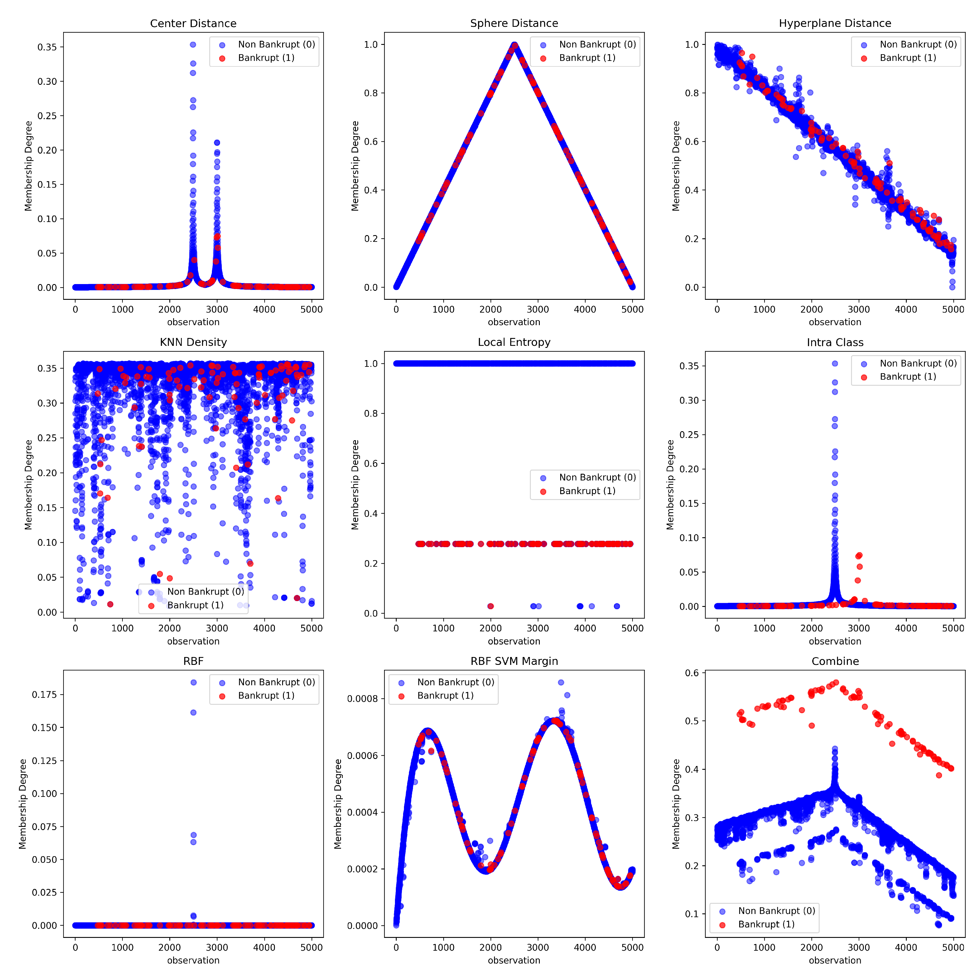
Figure 2.
Three visualizations of the used datasets: (a) Data1, (b) Data2, (c) Data3.
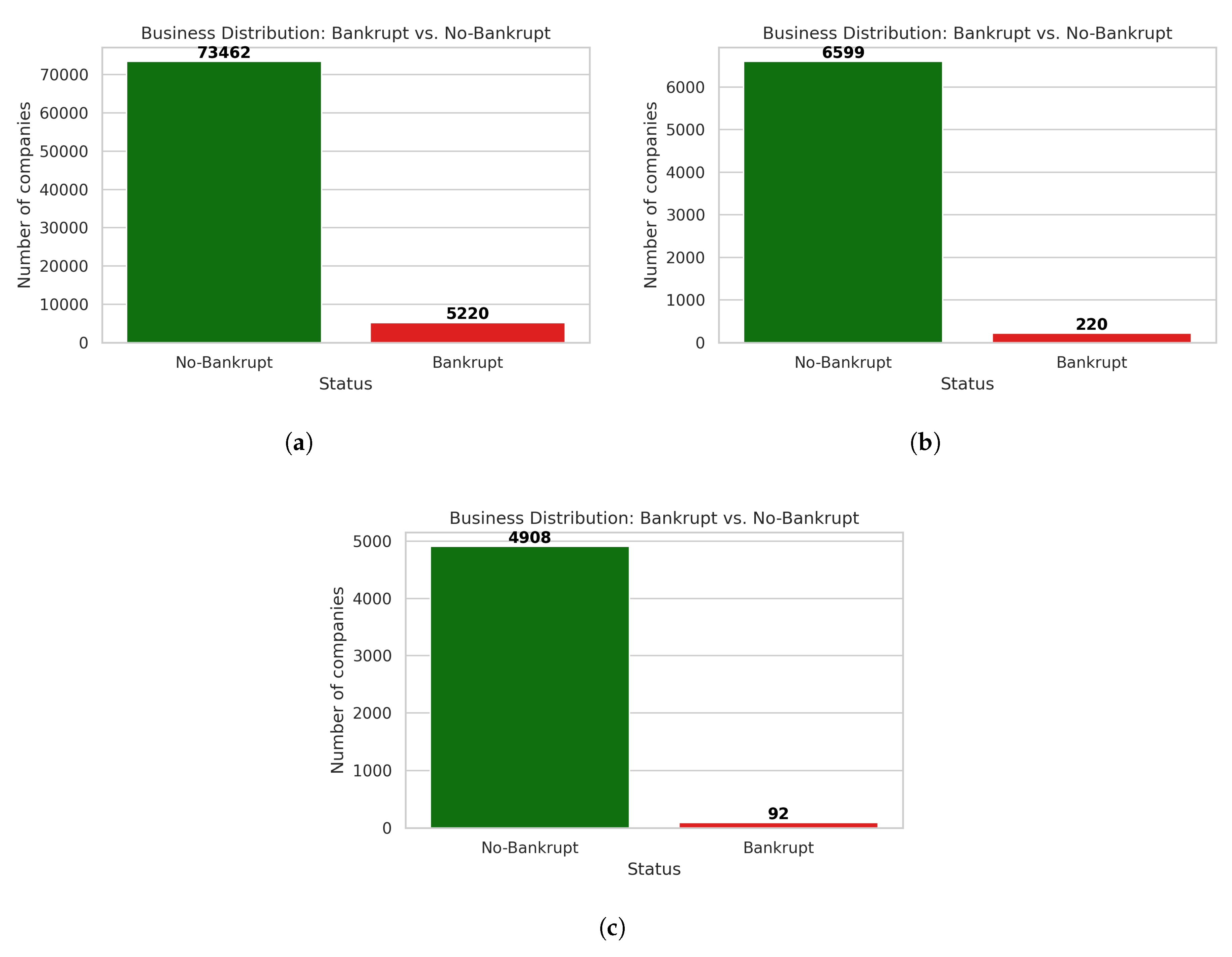
Table 1.
Classification performance of Fuzzy SVM variants and benchmark models.
| Model | Accuracy | F1-score | AUC-ROC | Precision | Recall | Specificity | G-mean |
|---|---|---|---|---|---|---|---|
| Fuzzy SVM (Centre) | 0.9530 | 0.0408 | 0.7010 | 0.0323 | 0.0556 | 0.9695 | 0.2321 |
| Fuzzy SVM (Sphere) | 0.9550 | 0.0000 | 0.7043 | 0.0000 | 0.0000 | 0.9725 | 0.0000 |
| Fuzzy SVM (Hyperplan) | 0.9550 | 0.0000 | 0.7058 | 0.0000 | 0.0000 | 0.9725 | 0.0000 |
| Fuzzy SVM (knn_density) | 0.9550 | 0.0426 | 0.7025 | 0.0345 | 0.0556 | 0.9715 | 0.2323 |
| Fuzzy SVM (local_entropy) | 0.9470 | 0.0000 | 0.7282 | 0.0000 | 0.0000 | 0.9644 | 0.0000 |
| Fuzzy SVM (intra_class) | 0.9540 | 0.0417 | 0.7133 | 0.0333 | 0.0556 | 0.9705 | 0.2322 |
| Fuzzy SVM (rbf) | 0.9580 | 0.0455 | 0.7531 | 0.0385 | 0.0556 | 0.9745 | 0.2327 |
| Fuzzy SVM (rbf_svm_margin) | 0.9520 | 0.0400 | 0.7037 | 0.0312 | 0.0556 | 0.9684 | 0.2320 |
| Fuzzy SVM (combined) | 0.9620 | 0.1764 | 0.8374 | 0.3154 | 0.1667 | 0.9766 | 0.4034 |
| DEC | 0.9520 | 0.0400 | 0.7021 | 0.0312 | 0.0556 | 0.9684 | 0.2320 |
| SVM-SMOTE | 0.9000 | 0.1525 | 0.8163 | 0.0900 | 0.1001 | 0.9073 | 0.2735 |
| SVM-ADASYN | 0.8280 | 0.1134 | 0.7463 | 0.0625 | 0.0111 | 0.8320 | 0.3130 |
| SVM-Undersampling | 0.7720 | 0.1024 | 0.8280 | 0.0551 | 0.0222 | 0.7729 | 0.3471 |
| Random Forest | 0.9020 | 0.0000 | 0.6211 | 0.0000 | 0.0000 | 0.7000 | 0.0000 |
| KNN | 0.9010 | 0.0000 | 0.6068 | 0.0000 | 0.0000 | 0.7980 | 0.0000 |
| Logistic Regression | 0.9020 | 0.0000 | 0.6626 | 0.0000 | 0.0000 | 0.6001 | 0.0000 |
Table 6.
Performance Comparison of Fuzzy Shadowed SVM and Other Models.
| Model | Accuracy | F1-score | AUC-ROC | Precision | Recall | Specificity | G-mean |
|---|---|---|---|---|---|---|---|
| Fuzzy Shadowed-center | 0.9142 | 0.3314 | 0.9028 | 0.2214 | 0.6591 | 0.9227 | 0.7798 |
| Fuzzy Shadowed-sphere | 0.9282 | 0.3553 | 0.9168 | 0.2500 | 0.6136 | 0.9386 | 0.7589 |
| Fuzzy Shadowed-hyperplane | 0.9289 | 0.3660 | 0.9187 | 0.2569 | 0.6364 | 0.9386 | 0.7729 |
| Fuzzy Shadowed-combined | 0.9699 | 0.3051 | 0.8663 | 0.6000 | 0.2045 | 0.9955 | 0.8290 |
| DEC | 0.9377 | 0.3609 | 0.9185 | 0.2697 | 0.2455 | 0.9508 | 0.3201 |
| SVM-SMOTE | 0.9304 | 0.3537 | 0.9119 | 0.2524 | 0.2909 | 0.9417 | 0.3459 |
| SVM-ADASYN | 0.8915 | 0.2745 | 0.9078 | 0.1750 | 0.2364 | 0.9000 | 0.3568 |
| SVM-Undersampling | 0.8409 | 0.2644 | 0.9213 | 0.1554 | 0.2864 | 0.8394 | 0.3626 |
| Random Forest | 0.9692 | 0.2759 | 0.9368 | 0.5714 | 0.1818 | 0.8955 | 0.2254 |
| KNN | 0.9507 | 0.2857 | 0.7424 | 0.6667 | 0.1818 | 0.8970 | 0.2258 |
| Logistic Regression | 0.9633 | 0.2188 | 0.8733 | 0.3500 | 0.1591 | 0.8902 | 0.2969 |
Disclaimer/Publisher’s Note: The statements, opinions and data contained in all publications are solely those of the individual author(s) and contributor(s) and not of MDPI and/or the editor(s). MDPI and/or the editor(s) disclaim responsibility for any injury to people or property resulting from any ideas, methods, instructions or products referred to in the content. |
© 2025 by the authors. Licensee MDPI, Basel, Switzerland. This article is an open access article distributed under the terms and conditions of the Creative Commons Attribution (CC BY) license (http://creativecommons.org/licenses/by/4.0/).
Copyright: This open access article is published under a Creative Commons CC BY 4.0 license, which permit the free download, distribution, and reuse, provided that the author and preprint are cited in any reuse.


