
Submitted:
26 May 2025
Posted:
27 May 2025
You are already at the latest version
Abstract
Over the past years, the field of Machine and Deep Learning has seen a strong 1
developments both in terms of software and hardware with the increase of specialised devices. One of the biggest challenges in this field is the inference phase, where the trained model makes predictions of unseen data. Although computationally powerful, traditional computing architectures face limitations in efficiently managing requests, especially from an energy point of view. For this reason, the need arose to find alternative hardware solutions and among these there are Field Programmable Gate Arrays (FPGAs): their key feature of being reconfigurable, combined with parallel processing capability, low latency and low power consumption, makes those devices uniquely suited to accelerating inference tasks. In this paper, we present a novel approach to accelerate the inference phase of a Multi-Layer Perceptron (MLP) using BondMachine , an OpenSource framework for the design of hardware accelerators for FPGAs. Analysis of the latency, energy consumption and resource usage as well as comparisons with respect to standard architectures and other FPGA approaches are presented, highlighting the strengths and critical points of the proposed solution.
Keywords:
BondMachine
; Reconfigurable computing
; Hardware-software co-design
; Low latency DNN Inference on 16 FPGA
; Low-power DNN Inference on FPGA
; DNN Accelerator
1. Introduction
Machine learning (ML) algorithms [2], particularly Deep Neural Networks (DNN), have witnessed remarkable achievements across diverse domains, ranging from computer vision and natural language processing to autonomous systems and recommendation systems [3]. Today, more specifically, ML techniques, more specifically DNN, are widely used in many scientific fields [4,5,6,7]. However, these advances often come at the cost of increased computational complexity, memory requirements, and power consumption. Moreover, the demand for ML in edge applications, where computational resources are typically limited, has further increased these requirements [8]. To address these challenges, researchers have been exploring techniques to optimize and streamline machine learning models. The main target of these techniques is the choice of data representation. On one hand, it has to be chosen considering the available hardware optimization available on the edge device. On the other hand, it has to be sufficiently precise to not compromise the accuracy of the model and as small as possible to reduce memory and computation requirements [9]. Indeed, it is a common technique to decrease the numerical precision of computations within ML tasks with respect to the standard 32-bit floating-point representation. By reducing the number of bits used to represent numerical values, it is possible to achieve more efficient storage, faster computation, and potentially lower energy consumption [10,11,12]. However, this approach is not without its drawbacks, and a careful analysis of the pros and cons is crucial to understand the implications of decreased numerical precision.
All the above mentioned aspects in terms of hardware optimization, can be achieved using FPGA devices. Several works have been published in recent years about the use of FPGAs to accelerate workloads and on FPGA-based heterogeneous computing systems [13,14,15,16].
In the present work we aim to use the BondMachine (BM) framework [1] to implement ML models on FPGA devices [17,18], and to analyze the effects of reduced numerical precision on the performance of the models, on the accuracy of the results, on the resource utilization and on the power consumption.
This study is part of a larger research project aimed at developing a new generation of heterogeneous computing systems for different applications, including edge AI. Our approach is to create a multi-core and heterogeneous ’register machine’ abstraction that can be used as an intermediate layer between the software applications and the FPGA hardware. From the software point of view, the BM offers a common interface that hides the specific FPGA hardware details, allowing a vendor independent development of the applications. From the FPGA point of view, the BM inherits the flexibility and parallelism of the FPGA devices. A similar approach has been used in software development with the introduction of the LLVM compiler infrastructure [19]. The LLVM VM is used as an intermediate layer between the high-level language and the architecture specific machine code. Most optimizations are performed at the LLVM level, and the final machine code is generated by the LLVM compiler. The BM is designed to be used in the same way, but for FPGA devices. Most optimizations are performed at the BM level, and the final FPGA configuration is generated by the BM tools.
Our focus is to provide a comprehensive evaluation of the benefits and limitations associated with this approach, shedding light on its impact on model performance, resource utilization, and overall efficiency. The increasing demand for edge AI applications, combined with the need for efficient and low-power computing systems, makes this research particularly relevant and timely, as it provides a new perspective on the design and implementation of AI accelerators for edge computing.
The present paper is organized as follows: in Section 2 we will first recall the basic components of the BM architecture, together with the basic tools of the BM software framework; then we describe the improvements we made to the BM ecosystem to allow the use of DNN models. In the subsequent section, that is Section 3.4, we will describe how a BM can be used to implement a DNN model on a FPGA, specifically we will give here all the details related to the mapping of a DNN on a BM, using a simple test model. In this section we will report all the test performed to deeply understand the impact of reduced precision algebra both in terms of computational deficiency, as well as in terms of the numerical precision. Finally, in Section 4 we will present the results we obtained using the LHC jet-tagging datasets using the Xilinx/AMD ALVEO [20] FPGA. Thus we will clearly draw some general conclusions.
2. Overview of the BondMachine Architecture
The BM project aims to enable a user to create a domain specific hardware as part of the development process all together with the software stack. In this context, FPGA technology allows to create independent processing units on a single low-power board, and to design their interconnections “in silicon” to maximally fit the design needs. In addition, as we will show, the BM’s architecture fits particularly well the computational structures of the DNNs and tensor processing models. In the following, we will firstly recall (sec:arch and sec:archhandling) all the basic logical components of the BM architecture as well as the basic tools of the BM software framework already detailed in our previous work [1]. We will instead describe all the improvements we made to the BM ecosystem to allow the implementation of DNN models in Section sec:modifications.
2.1. Architecture Specification
As already stated, the main goal of the BM is to start from a high level specification of a generic computational task and to produce both the hardware, specified as an HDL to be used for the FPGA, and the software that will run on the hardware. The basic logical elements of each BM architecture are: the Connecting Processor (CP), and the Shared Objects (SOs).
The CPs are the computational cores of the BM. Each CP implements all the needed instructions to solve the given computational task that has been assigned. Thus, it should be clear as the heterogeneity of the BM is pushed down to the level of the computational core. Indeed, each CP can be highly specialized to execute only those operations strictly needed, that is: a CP is as simple as possible, and it is specialized to perform a task and eventually specially optimized for it.
Clearly, to solve complex tasks many CPs must collaborate and share information and resources. This is exactly where the SOs start to play a fundamental role increasing the processing capability and functionality of the BM. At the present stage of the project there are different SOs: Channels, Shared Memories, Barriers, Pseudo Random Numbers Generator, Shared queues and stacks (the reader may refer to our previous work [20] for all the details).
2.2. Architecture Handling
To properly handle all the basic operations behind a BM creation and management we developed a set of software tools. At the bottom there are the procbuilder and the bondmachine builder. While the first is devoted controlling every aspect regarding the creation and management of each CP, the latter is used to configure the interconnections between all the CPs and SOs constituting a BM. On top of the BM architecture handling framework there is the bondgo arch compiler. This compiler, starting from a Go[21] source code, will generate both the specific optimal BM, as well as the application that will run on it. That is: starting from a Go source code the final user has the capability to produce both the optimal BM architecture (i.e. machine), as well as the optimal application to solve the given computational task.
3. Strategy and Ecosystem Improvements to Accelerate DL Inference Tasks
Our strategy to accelerate DL inference tasks within the BM ecosystem is based on a dynamic and adaptable architecture design. Each CP executes an Instruction Set Architecture (ISA) that combines statically defined operations with dynamic instructions generated at run time, such as those for Floating-Point (FloPoCo) opcodes and Linear Quantization. This approach, along with a fragment-based assembly methodology via the BM Assembler (BASM), enables the creation of specialized computing units tailored to diverse Neural Network related operations.
Additionally, the BM ecosystem offers a unified handling of heterogeneous numerical representations through the bmnumbers package, and provides tools such as Neuralbond, TensorFlow Translator, and NNEF composer to translate DNN models into BM architectures. Support for multiple FPGA platforms (e.g., Digilent Zedboard, Xilinx/AMD ALVEO) and a high-level Python library further simplify interaction, prototyping, and deployment of FPGA-based accelerators.
3.1. A Flexible ISA: Combining Static and Dynamic Instructions
Each CP of a BM is able to execute some instructions forming a specific ISA. The ISAs, one for each CP, are composed choosing from a set of available instructions. For example, to perform a sum between two numbers, the CP must be able to execute the add instruction. Some instructions act on specific data types; for example, the add instruction can be used to sum two integers, addf to sum two floating point numbers, and so on.
Apart from the basic instructions, which are statically defined within the project, each CP also executes dynamic instructions. A Dynamic Instruction is an opcode that is not statically defined within the project, but it is dynamically generated at run-time. It can be, for example, HDL code generated by an external tool or an instruction that changes according to the input. Examples of dynamic instructions are Floating-Point Cores (FloPoCo) (i.e., a generator of Floating-Point, but not only, cores for FPGAs)[22] opcodes that are generated by the FloPoCo tool and Linear Quantization [23] opcodes.
3.2. Extending Numerical Representations in the BM Ecosystem: FloPoCo, Linear Quantization and the Bmnumbers Package
FloPoCo [22,24] is an open-source software tool primarily used to automatically generate efficient hardware implementations of floating-point operators for FPGAs. FloPoCo has been integrated within the BM ecosystem to allow the use of optimized floating point operators. We aim to provide a comprehensive evaluation of the benefits and limitations associated with this approach, shedding light on its impact on model performance, resource utilization, and overall efficiency. One of the main features of this framework is the representation of floating point numbers using an arbitrary precision, i.e., number of bits. In fact, it is possible to arbitrarily choose the number of bits assigned to both the exponent and the mantissa. This leads to great freedom in selecting numerical precision, allowing us to perform various tests by varying the number of bits used to represent a floating-point number.
Linear Quantization is a technique that allows one to represent a floating point number using a fixed number of bits and integer arithmetic [23]. The BM ecosystem has been extended to allow the use of Linear Quantization operators. The main advantage of this approach is the possibility to use integer arithmetic, which is much more efficient than floating-point arithmetic on FPGA devices. In order to achieve this, special dynamic instructions were developed for this type of operators.
Finally, given the heterogeneity of the BM and the different numerical representations that can be used, it is necessary to have a common way to represent numerical values in both the software layer and the hardware. The bmnumbers package has been developed exactly to achieve this goal. This package is a Go library that manages all the numerical aspects of the BM. In particular, it is able to parse a numerical representation (i.e. a string) and to produce the corresponding binary representation (i.e., a slice of bits). This is achieved using a prefix notation, where the first characters of the string are used to identify the numerical representation. For example, the string “0f0.5” is parsed as a floating point number, or “0lq0.5<8,1>” is parsed as a linear quantized number of 8 bits with ranges given by type 1 (the type is stored as an external data structure within bmnumbers). Table 1 reports the available numerical representations and the corresponding prefix.
It is importa to underline as bmnumbers is also responsible for the conversion, casting, and export of numerical representations throughout the BM ecosystem.
3.3. BASM and Fragments
The BM ecosystem has been extended to allow the use of a new tool called BASM (BondMachine Assembler). BASM uses a low level language that allows one to write BM code directly in assembly. Similarly to the BondGo compiler, BASM is able to generate both the BM architecture and the application that will run on it.
A central concept of BASM is the fragment. Fragments are small pieces of code that can be assembled in different ways to form more complex code to end up in a complete BM architecture. By acting on some metadata it is possible to change how the fragments are mapped to the CPs and how they are connected to each other, allowing for the creation of different BM architectures starting from the same fragments. For example, a group of fragments can be mapped to a single CP, or each fragment can be mapped to a different CP. In the first case the fragments will be executed sequentially, in the latter they will be executed in parallel on different CPs. Moreover, the assembly language in BASM supports the use of templates. In such a way, the code can be generic and can be instantiated with different parameters. This can be used, for example, to change data type or to change the number of bits used to represent a number.
3.4. Mapping a DNN as an Heterogeneous Set of CPs
A BM can be used to solve any computational task, but in fact the interconnected heterogeneous processors model, on which any BM is based, seems to be ideal for mapping a DNN [25].Thus, we developed three different tools to be used to map a DNN model to a proper BM architecture: Neuralbond, Tensorflow Translator and NNEF composer [1]. In the present work we used the Neuralbond tool, that starting from the NN architecture it builds a BM composed by several CPs acting as one or more neuron-like computing units. The Neuralbond approach is Fragment-based, thus: each generated CP is the composition of one or more BASM fragments taken from a library we created, and each fragment contains the code to perform the computation of a single neuron.
An example of the softmax neuron written in Basm is shown in the following code snippet:
List 1.
Fragment template for a softmax neuron.
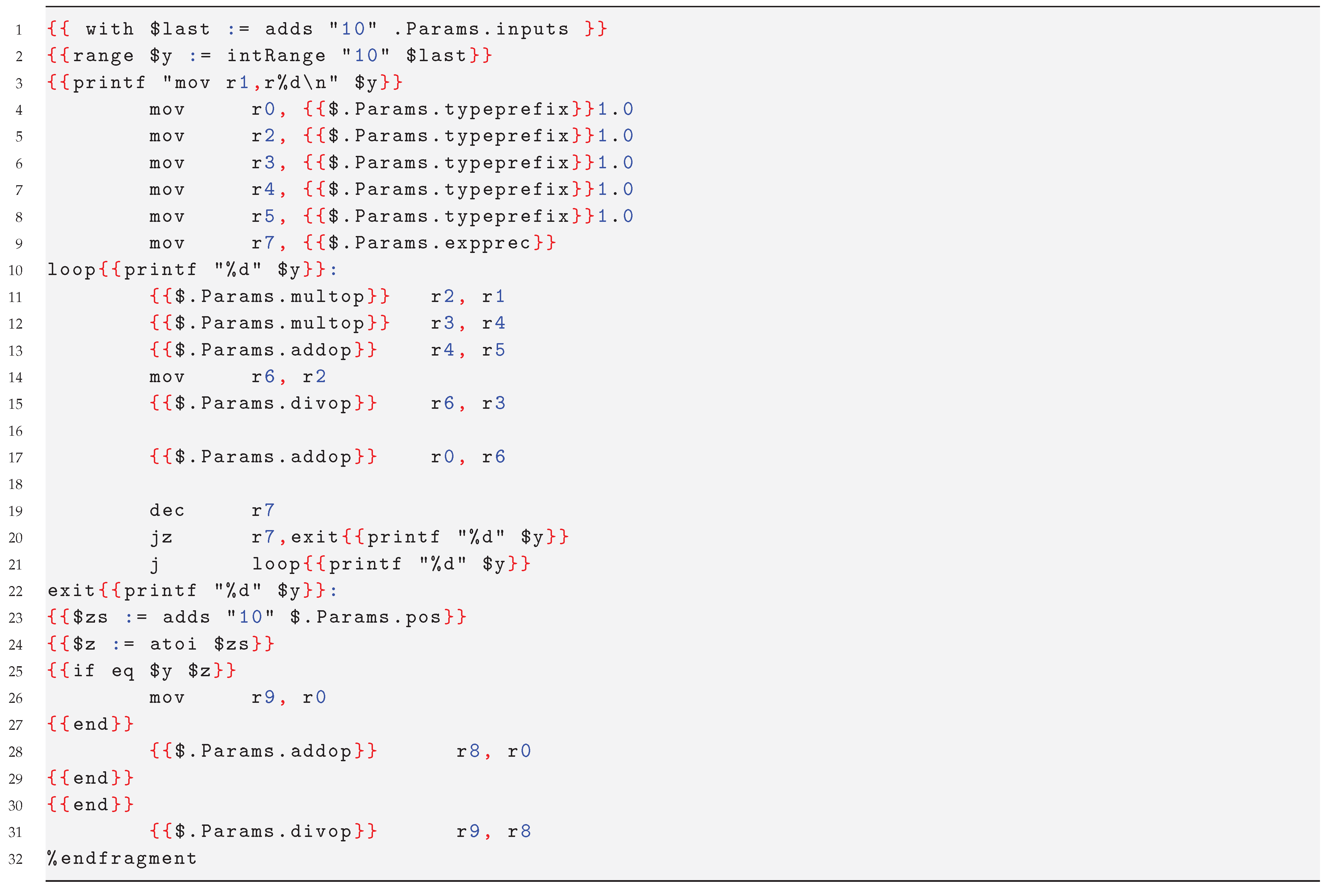
BASM takes this fragment and generates a complete computational unit capable of performing the specified operation. Neuralbond then iterates over the neurons and weights of the DNN, leveraging BASM to construct the final BM architecture that implements the entire DNN. This methodology enables the customization of neurons according to the specific requirements of the use case. As an example, consider the fragment mentioned previously that implements the softmax function. This fragment was developed following the corresponding mathematical formulation.
where K in the formula 2 is the expprec, that is the number of iterations of the Taylor series expansion of the exponential function. As K increases, the series includes more terms, making the approximation of more accurate. Each term in the series brings the approximation closer to the true value of . However, calculating more terms also increases the computational cost. For example, if , the Taylor expansion is truncated after the first two terms:
than is poorly approximated and the Softmax output will also be inaccurate since it is sensitive to the exponential value (i.e., it determines how the probabilities are distributed among the classes). The trade-off between accuracy and computational cost is an important consideration when selecting the value of K, as it affects the performance of the model. A detailed analysis of the impact of the expprec parameter has been conducted using a simplified test model (such as that reported in Figure 1) and a related dataset, and all results of this investigation are reported in SI. Based on these analyses it was observed that the softmax function is highly sensitive to the number of terms used in the Taylor series expansion of the exponential function, particularly under conditions of reduced numerical precision. For example, when using the standard 32-bit IEEE 754 floating-point representation, setting the expprec parameter to 1 is generally sufficient to preserve model accuracy. In contrast, when 16-bit precision FloPoCo operators are used, a higher value of expprec, typically between 2 and 10, is required to achieve comparable accuracy. Deviating from this optimal range, either by decreasing or excessively increasing the value of expprec, leads to a significant degradation in model performance. This finding underscores the importance of balancing computational efficiency and numerical accuracy, especially in resource-constrained environments or hardware-limited implementations. In the benchmarks described in Section 4, we reduced this exponent to its minimum value, trading off accuracy for improved performance.
To better understand how the DNN mapping on a BM is performed, consider a multilayer perceptron (MLP) designed to solve a classification problem. This network has 4 input features, a single hidden layer with one neuron using a linear activation function, and an output layer with 2 neurons employing the softmax activation function, as shown in Figure 1.
The resulting BM architecture, reported in Figure 2, is made up of 4 inputs (that is, the number of features) and 2 outputs (i.e., the classes). It consists of 33 connecting processors, including: 4 CPs for reading the incoming inputs, 12 CPs corresponding to the "weights" and performing the multiplication between the input and its associated weight, 1 CP that executes the linear function, 2 CPs performing the softmax functions, and 2 CPs to write the final computed output values. The total number of registers in the CPs is 80, while the total number of bonds is 30.
Theoretically, by implementing every possible type of neuron within the library, any DNN can be mapped to a BM architecture and synthesized on an FPGA.
3.5. BM as Accelerator
In addition to the core modifications made to the BM framework, further enhancements have extended the automation mechanisms to support heterogeneous hardware platforms, including the Digilent Zedboard (Soc: Xilinx Zynq-7000 [27]) and Xilinx/AMD ALVEO [20] boards. The latter are well known for their high resource availability and performance in accelerated computing. In particular, they are increasingly being adopted for the deployment of advanced DL systems [26].
To deploy the architecture created as an accelerator for a host running a standard Linux operating system, the BM ecosystem leverages the AXI protocol [27] for communication. AXI is a widely adopted standard for interfacing with FPGA devices and facilitates the integration of all available tools for FPGA accelerator development.
In particular, both the AXI Memory Mapped (AXI-MM) protocol and the AXI Stream protocol have been successfully implemented and can be used to interact with the BM architecture running on the FPGA, depending on the specific requirements and the use case. For example, AXI-MM can be preferred when memory access patterns dominate the application, while AXI Stream is more suitable for continuous data-flow processing.
Furthermore, a high-level Python library, pybondmachine, has been developed to facilitate interaction with the BM framework, as well as with FPGA devices programmed using the BM toolkit, thereby streamlining the deployment and management of hardware-accelerated applications.
3.6. Real-Time Power Measurement and Energy Profiling
As noted in the Introduction, power consumption is nowadays a critical factor when designing a DNN accelerator on an FPGA. Even if energy consumption in DL involves both training and inference phases, in production environments inference dominates running costs, accounting for up to 90 % of total compute cost [11,12]. Deploying specialized, energy-efficient hardware, such as FPGAs, therefore, represents an effective strategy for reducing this overhead.
The tools supplied by Xilinx provide the ability to analyze the energy usage of a given design by producing a detailed report with estimated power figures. Within the BM framework, we have implemented the necessary automation to extract these data and generate a concise summary report. However, while Vivado’s summary reports are useful for obtaining a general overview of the power profile of a design, direct real-time measurement of energy consumption is essential to evaluate its true impact.
To this end, we implemented a real-time power-measurement setup on the ZedBoard powered by a 12 V stabilized supply and monitored via a high-resolution digital multimeter, in order to separate static (leakage) from dynamic (switching) power of the inference IP alone. Dynamic power is modeled as
Analysis across FloPoCo floating-point precisions of 12, 16, 19 and 32 bits reveals a marked increase in both static and dynamic power with bit-width, yielding energy per inference from 0.8 × 10⁻⁷ J (12 bits) to 3.8 × 10⁻⁷ J (32 bits).
In addition, a comparative study on CPU platforms has been conducted and the results are summarized in Table 2.
The study on CPU platforms demonstrates that FPGAs deliver inference times on the order of s, comparable to the Intel CPU but with up to three orders of magnitude lower energy consumption; relative to the ARM processor, FPGA inference is slower ( s) yet still substantially more energy-efficient. Additional detailed results of the power consumption and of the setup used are reported in SI.
4. Benchmarking the DL Inference FPGA-Based System for Jet Classification in LHC Experiments
DNNs are widely used in the field of high-energy physics [28], for instance, they are used for the classification of jets produced in the collisions of the Large Hadron Collider (LHC) at CERN [29]. However, in this context, FPGAs are primarily used in the trigger system of the LHC experiments to make a real-time selection of the most interesting events to be stored. Thus, the use of DNN in FPGA is a promising solution to improve the performance of the trigger system and to find novel ways to reduce both the latency of the trigger system and energy consumption, which are crucial factors in this scenario.
The complexity of the DNN involved is balanced to meet the rigid requirements of FPGA-based trigger systems at LHC. Specifically, the Level-1 Trigger system must process data at a rate of 40 MHz and make decisions within a latency of approximately 12.5 microseconds, necessitating the use of DNNs that are optimized for low latency and efficient resource utilization [30]. Methods such as compressing DNNs by reducing numerical precision have been used to reduce processing times and resource utilization while preserving model accuracy [31].
To evaluate the effectiveness of the proposed solution, benchmarks were performed using the LHC jet tagging dataset [34], a well-known resource in the field of high-energy physics, and it is used to classify jets produced in the collisions at LHC. The dataset is composed of 100000 jets, each with 16 features and the classification task is to identify if a jet is a gluon, a quark, a W boson or a Z boson and top quark.
The selected DNN architecture (see Figure 3) consists of 16 input neurons, three hidden layers with 64, 32, and 32 neurons respectively, employing the Linear activation function, and 5 output neurons using the Softmax activation function. To test the proposed model, the Alveo U55C board has been chosen, which offers high throughput and low latency for DL inference tasks.
The benchmarking process involved systematically varying the numerical precision of the model, made possible through the integration of the FloPoCo library. The evaluation focused on three critical metrics: resource utilization, measured in terms of Look-Up Tables (LUTs), Registers (REGs) and Digital Signal Processors (DSPs); latency, defined as the time required to perform a single inference; and precision, quantified as the deviation of the predictions of the FPGA-implemented model from the ground truth. Adjusting numerical precision is a commonly adopted technique for reducing a model’s energy consumption. In this context, a real-world power consumption analysis was performed to assess the effect of FloPoCo numerical precision on the model’s power usage, as mentioned in Section 3.6. The detailed results of the power consumption analysis are presented in SI.
The benchmark results, summarized in Table 3, reveal critical points in the performance and resource utilization of various numerical precision formats when implemented on the Alveo U55C FPGA. Concerning resource utilization, the float32 format, which adhered to the IEEE754 standard, exhibits the highest utilization of LUTs at 476416, accounting for 36.54% of the FPGA’s available resources. As the precision is reduced to lower bit widths (e.g., float16, flpe5f11, flpe6f10), LUT usage decreases, with the flpe6f4 format requiring only 274523 LUTs, which corresponds to 21.06% of the available resources. This suggests that lower-precision formats tend to be more efficient in terms of LUT utilization.

Table 3.
Resource utilization, including Look-Up Tables (LUTs), Registers (REGs), and Digital Signal Processors (DSPs), along with latency and accuracy for different data types implemented on the Alveo U55C FPGA. The float32 and float16 formats adhere to the IEEE754 standard, while the flpe variants employ custom precision formats from the FloPoCo library. The fixed<16,8>format represents a fixed-point configuration.
| Data Type | LUTs | REGs | DSPs | |||
|---|---|---|---|---|---|---|
| Count | (%) | Count | (%) | Count | (%) | |
| float32 | 476416 | 36.54 | 456235 | 17.50 | 954 | 10.57 |
| float16 | 288944 | 22.16 | 298191 | 11.44 | 479 | 5.31 |
| flpe7f22 | 423915 | 32.52 | 352113 | 13.50 | 950 | 10.53 |
| flpe5f11 | 393657 | 30.20 | 318821 | 12.23 | 477 | 5.29 |
| flpe6f10 | 442809 | 33.97 | 334414 | 12.83 | 4 | 0.04 |
| flpe4f9 | 347633 | 26.67 | 275653 | 10.57 | 4 | 0.04 |
| flpe5f8 | 299033 | 22.94 | 261403 | 10.03 | 4 | 0.04 |
| flpe6f4 | 274523 | 21.06 | 236429 | 9.07 | 4 | 0.04 |
| fixed<16,8> | 205071 | 15.73 | 207670 | 7.94 | 477 | 5.29 |
| Data Type | Latency ( ) | Accuracy (%) |
|---|---|---|
| float32 | 12.29 ± 0.15 | 100 |
| float16 | 8.65 ± 0.15 | 99.17 |
| flpe7f22 | 6.23 ± 0.18 | 100.00 |
| flpe5f11 | 4.46 ± 0.21 | 100.00 |
| flpe6f10 | 4.49 ± 0.18 | 100.00 |
| flpe4f9 | 2.80 ± 0.15 | 97.78 |
| flpe5f8 | 3.31 ± 0.12 | 99.74 |
| flpe6f4 | 2.72 ± 0.23 | 96.39 |
| fixed<16,8> | 1.39 ± 0.06 | 86.03 |
Similar trends are observed for the utilization of REGs, with the float32 format requiring the largest number of registers (456235, or 17.50%). As precision is reduced, the number of registers used decreases, with the fixed<16,8> format utilizing only 207670 REGs, or 7.94%. This reduction in resource usage is consistent with the general behavior expected from lower-precision formats, which require fewer resources for computation. DSP utilization remains relatively low for most formats. The float32 and float16 formats require 954 and 479 DSPs, respectively. In contrast, the lower-precision flpe formats (e.g., flpe6f4) utilize a minimal number of DSPs (just 4), highlighting the significant reduction in DSP resource requirements when lower-precision custom formats are employed.
The results of the latency show that the float32 format exhibits the highest latency (12.29 ± 0.15), which is expected as higher precision computations generally involve more complex operations, leading to increased computation burden. As precision decreases, latency also decreases. For example, the latency for the flpe6f4 format is reduced to 2.72 ± 0.23, demonstrating a performance improvement with lower precision. Moreover, the fixed<16,8> format shows the lowest latency (1.39 ± 0.06), indicating that fixed-point precision can offer significant speed advantages for certain tasks.
The accuracy of the models is measured as the deviation between the predictions of the FPGA-implemented model and the ground truth. In general, all the floating-point precision formats, including float32, float16, and the various FloPoCo-based formats, exhibit high accuracy, with values approaching or exceeding 99%. Among the FloPoCo-based formats, accuracy is further improved. The flpe7f22, flpe5f11, and flpe6f10 formats each achieve 100% accuracy, demonstrating that FloPoCo-based representations can match or even surpass the precision of conventional floating-point formats. Furthermore, these formats are particularly advantageous, as they reduce resource utilization and latency while maintaining optimal accuracy, demonstrating the effectiveness of FloPoCo in custom DNN implementations. On the other hand, the fixed <16,8>format, which uses fixed point arithmetic and still under development, shows a significant reduction in precision, achieving only 86.03%. This decrease can be attributed to the inherent limitations of fixed-point arithmetic, where rounding errors accumulate, leading to a less precise model.
4.1. Comparing HLS4ML and BM
Performing ML inference on FPGA is a goal pursued by several frameworks. Among these, one of the most well-known is High-Level Synthesis for Machine Learning (HLS4ML) [32], designed to translate ML models trained in high-level languages like Python or TensorFlow into custom hardware code for FPGA hardware acceleration. Therefore, we chose to evaluate our solution by benchmarking it against the HLS4ML approach, using the same DL model described in Figure 3, the LHC jet dataset and the ALVEO U55C FPGA. HLS4ML also offers various options in terms of numerical precision, and for our comparison, we chose to use the default numerical precision set by the library itself during the high-level configuration phase, specifically using a fixed-point representation with a total of 16 bits, 6 of which are allocated for the fractional part. Moreover, HLS4ML offers multiple strategies for firmware generation. We selected the default option, called Latency, which prioritizes performance over resource efficiency. HLS4ML, thanks to the drivers it provides for interaction between the PS (Processing System) and PL (Programmable Logic) parts, returns metrics about the inference time. Although the resulting timing depends on the batch size selected, the best results obtained for a single classification are reported in the Table 4.
Compared to the system presented, the HLS4ML solution is more efficient in terms of overall resource utilization and performance compared to the BM solution. Specifically, the HLS4ML implementation with fixed<16,6>precision achieves a low inference latency of 0.17 ± 0.01 , which is an order of magnitude faster than the best latency achieved by the BM approach (1.39 ± 0.06 using the same fixed-point configuration). While the BM design using floating-point precision formats achieves accuracy values close to or even at 100%, and the fixed-point BM implementation reaches 81.73%, the HLS4ML fixed-point design achieves an intermediate accuracy of 95.11%. This indicates that while HLS4ML’s optimizations for resource usage and latency result in excellent performance and hardware efficiency, they also introduce some loss of precision, likely due to the quantization effects associated with its default fixed-point configuration.
The comparison with HLS4ML was made to assess the overhead introduced by the BM layer, which requires more resources for the same numerical precision while maintaining similar performance in terms of latency. In order to well interpret these results, we need to underline here, once more, that the BM provides a new kind of computer architecture, where the hardware dynamically adapts to the specific computational problem rather than being static and generic, and the hardware and software are co-designed, guaranteeing a full exploitation of fabric capabilities. Although the HLS4ML solution exceeds the proposed approach in terms of resource efficiency, it lacks the same level of flexibility and general-purpose adaptability. In contrast, the BM ecosystem offers greater versatility. As an open-source, vendor-independent platform, BM enables the deployment of the same NN model across different boards while autonomously generating HDL code. This presents a significant advantage over other solutions, which are more constrained in terms of hardware compatibility and are often vendor-dependent, relying on board-specific tools to generate low-level HDL code. Additionally, BM’s modular design ensures seamless integration with other frameworks and libraries, as demonstrated in this work with the integration of the FloPoCo library, making it highly adaptable to diverse hardware configurations. While HLS4ML proves to be more efficient for the current application, BM’s flexibility and extensibility establish it as a more versatile and scalable solution since it can seamlessly adapt to diverse hardware platforms, integrate specialized libraries, and meet evolving application requirements without being tied to vendor-specific tools or architectures.
5. Conclusions
In the present work, we described the developments and the updates done in the BondMachine OpenSource framework for the design of hardware accelerators for FPGAs, in particular for the implementation of machine learning models, highlighting its versatility and customizability. We demonstrated that the BM framework is a tool that can be used also to develop and port ML-based models to FPGAs (mainly MLP architectures), and has the capability of integrating different existing libraries for arithmetic precision.
The paper begins with a brief introduction to the BM framework, describing its main features and the main components. Then, we detailed how the framework has been extended to map a neural network multi layer perceptron model into a BondMachine architecture to perform inference on FPGA. We tested the solution proposed, discussing the results obtained and the optmizations done to improve the performance. Next, we have reported in detail the analyses of our implementation varying the numerical precision, both by integrating external libraries such as FloPoCo and by using well-known techniques like fixed-point precision, evaluating variations in terms of latency and resource utilization. We also reported some of the results about the energy consumption measurements, a key aspect in this context, describing the setup used and providing real measurements of the power consumption of the FPGA board, giving a comparison with the energy consumption of the same task performed on a standard CPU architecture.
Finally, we have compared our solution with respect to the HLS4ML one, a well-known framework for implementing machine learning inference on FPGA. Overall, this work establishes a methodology of testing and measurements for future developments of bigger and more complex models (i.e., we are indeed working on the implementation of Convolution NN), as well as for different FPGA devices, and it represents a first step towards the implementation of a complete and efficient solution for the inference of machine learning models on FPGA.
Acknowledgments
This work is partially supported by ICSC – Centro Nazionale di Ricerca in High Performance Computing, Big Data and Quantum Computing, funded by European Union – NextGenerationEU. L. S. acknowledges funding from “PaGUSci - Parallelization and GPU Porting of Scientific Codes” CUP: C53C22000350006 within the Cascading Call issued by Fondazione ICSC , Spoke 3 Astrophysics and Cosmos Observations. National Recovery and Resilience Plan (Piano Nazionale di Ripresa e Resilienza, PNRR) Project ID CN_00000013 "Italian Research Center on High-Performance Computing, Big Data and Quantum Computing" funded by MUR Missione 4 Componente 2 Investimento 1.4: Potenziamento strutture di ricerca e creazione di "campioni nazionali di R&S (M4C2-19 )" - Next Generation EU (NGEU).
References
- Mariotti, M.; Magalotti, D.; Spiga, D.; Storchi, L. The BondMachine, a moldable computer architecture. Parallel Computing 2022, 109, 102873. [Google Scholar] [CrossRef]
- Jordan, M.I.; Mitchell, T.M. Machine learning: Trends, perspectives, and prospects. Science 2015, 349, 255–260. [Google Scholar] [CrossRef] [PubMed]
- Abiodun, O.I.; Jantan, A.; Omolara, A.E.; Dada, K.V.; Mohamed, N.A.; Arshad, H. State-of-the-art in artificial neural network applications: A survey. Heliyon 2018, 4. [Google Scholar] [CrossRef] [PubMed]
- Storchi, L.; Cruciani, G.; Cross, S. DeepGRID: Deep Learning Using GRID Descriptors for BBB Prediction. Journal of Chemical Information and Modeling 2023, 63, 5496–5512. [Google Scholar] [CrossRef]
- Hong, Q.; Storchi, L.; Bartolomei, M.; Pirani, F.; Sun, Q.; Coletti, C. Inelastic N 2+ H 2 collisions and quantum-classical rate coefficients: large datasets and machine learning predictions. The European Physical Journal D 2023, 77, 128. [Google Scholar] [CrossRef]
- Hong, Q.; Storchi, L.; Sun, Q.; Bartolomei, M.; Pirani, F.; Coletti, C. Improved Quantum–Classical Treatment of N2–N2 Inelastic Collisions: Effect of the Potentials and Complete Rate Coefficient Data Sets. Journal of Chemical Theory and Computation 2023. [Google Scholar] [CrossRef]
- Tedeschi, T.; Baioletti, M.; Ciangottini, D.; Poggioni, V.; Spiga, D.; Storchi, L.; Tracolli, M. Smart Caching in a Data Lake for High Energy Physics Analysis. Journal of Grid Computing 2023, 21, 42. [Google Scholar] [CrossRef]
- Hua, H.; Li, Y.; Wang, T.; Dong, N.; Li, W.; Cao, J. Edge computing with artificial intelligence: A machine learning perspective. ACM Computing Surveys 2023, 55, 1–35. [Google Scholar] [CrossRef]
- Capra, M.; Bussolino, B.; Marchisio, A.; Masera, G.; Martina, M.; Shafique, M. Hardware and software optimizations for accelerating deep neural networks: Survey of current trends, challenges, and the road ahead. IEEE Access 2020, 8, 225134–225180. [Google Scholar] [CrossRef]
- Ngadiuba, J.; Loncar, V.; Pierini, M.; Summers, S.; Di Guglielmo, G.; Duarte, J.; Harris, P.; Rankin, D.; Jindariani, S.; Liu, M.; et al. Compressing deep neural networks on FPGAs to binary and ternary precision with hls4ml. Machine Learning: Science and Technology 2020, 2, 015001. [Google Scholar] [CrossRef]
- Thomas, D. Reducing machine learning inference cost for pytorch models 2020.
- Plumed, F.; Avin, S.; Brundage, M.; Dafoe, A.; hÉigeartaigh, S.; Hernandez-Orallo, J. Accounting for the Neglected Dimensions of AI Progress 2018.
- Samayoa, W.F.; Crespo, M.L.; Cicuttin, A.; Carrato, S. A Survey on FPGA-based Heterogeneous Clusters Architectures. IEEE Access 2023. [Google Scholar]
- Zhao, T. FPGA-Based Machine Learning: Platforms, Applications, Design Considerations, Challenges, and Future Directions. Highlights in Science, Engineering and Technology 2023, 62, 96–101. [Google Scholar] [CrossRef]
- Liu, X.; Ounifi, H.A.; Gherbi, A.; Li, W.; Cheriet, M. A hybrid GPU-FPGA based design methodology for enhancing machine learning applications performance. Journal of Ambient Intelligence and Humanized Computing 2020, 11, 2309–2323. [Google Scholar] [CrossRef]
- Ghanathe, N.P.; Seshadri, V.; Sharma, R.; Wilton, S.; Kumar, A. MAFIA: Machine learning acceleration on FPGAs for IoT applications. In Proceedings of the 2021 31st International Conference on Field-Programmable Logic and Applications (FPL). IEEE, 2021, pp. 347–354.
- Shawahna, A.; Sait, S.M.; El-Maleh, A. FPGA-based accelerators of deep learning networks for learning and classification: A review. ieee Access 2018, 7, 7823–7859. [Google Scholar] [CrossRef]
- Monmasson, E.; Cirstea, M.N. FPGA design methodology for industrial control systems—A review. IEEE transactions on industrial electronics 2007, 54, 1824–1842. [Google Scholar] [CrossRef]
- Lattner, C.; Adve, V. LLVM: A compilation framework for lifelong program analysis & transformation. Proceedings of the international symposium on Code generation and optimization: feedback-directed and runtime optimization, 2004; 75–88. [Google Scholar]
- Mariotti, M.; Storchi, L.; Spiga, D.; Salomonie, D.; Boccalif, T.; Bonacorsid, D. The BondMachine toolkit: Enabling Machine Learning on FPGA. In Proceedings of the International Symposium on Grids & Clouds 2019, 2019, 20. [Google Scholar]
- Meyerson, J. The go programming language. IEEE software 2014, 31, 104–104. [Google Scholar] [CrossRef]
- Dinechin, F.d.; Lauter, C.; Tisserand, A. FloPoCo: A generator of floating-point arithmetic operators for FPGAs. ACM Transactions on Reconfigurable Technology and Systems (TRETS) 2009, 2, 10. [Google Scholar]
- Gholami, A.; Kim, S.; Dong, Z.; Yao, Z.; Mahoney, M.W.; Keutzer, K. A survey of quantization methods for efficient neural network inference. In Low-Power Computer Vision; Chapman and Hall/CRC, 2022; pp. 291–326.
- de Dinechin, F.; Pasca, B. Designing Custom Arithmetic Data Paths with FloPoCo. IEEE Design & Test of Computers 2011, 28, 18–27. [Google Scholar] [CrossRef]
- Haykin, S. Neural networks. A comprehensive foundation 1994. [Google Scholar]
- Kljucaric, L.; George, A.D. Deep learning inferencing with high-performance hardware accelerators. ACM Transactions on Intelligent Systems and Technology 2023, 14, 1–25. [Google Scholar] [CrossRef]
- AMBA AXI Protocol Specification, 2023.
- Denby, B. The Use of Neural Networks in High-Energy Physics. Neural Computation 1993, 5, 505–549. [Google Scholar] [CrossRef]
- Cagnotta, A.; Carnevali, F.; De Iorio, A. Machine Learning Applications for Jet Tagging in the CMS Experiment. Applied Sciences 2022, 12. [Google Scholar] [CrossRef]
- Savard, Claire. Overview of the HL-LHC Upgrade for the CMS Level-1 Trigger. EPJ Web of Conf. 2024, 295, 02022. [CrossRef]
- Aarrestad, T.; Loncar, V.; Ghielmetti, N.; Pierini, M.; Summers, S.; Ngadiuba, J.; Petersson, C.; Linander, H.; Iiyama, Y.; Di Guglielmo, G.; et al. Fast convolutional neural networks on FPGAs with hls4ml. Machine Learning: Science and Technology 2021, 2, 045015. [Google Scholar] [CrossRef]
- Fahim, F.; Hawks, B.; Herwig, C.; Hirschauer, J.; Jindariani, S.; Tran, N.; Carloni, L.P.; Di Guglielmo, G.; Harris, P.; Krupa, J.; et al. hls4ml: An open-source codesign workflow to empower scientific low-power machine learning devices. arXiv preprint, 2021; arXiv:2103.05579. [Google Scholar]
Figure 1.
A DNN with one hidden layer, 4 inputs and 2 outputs.
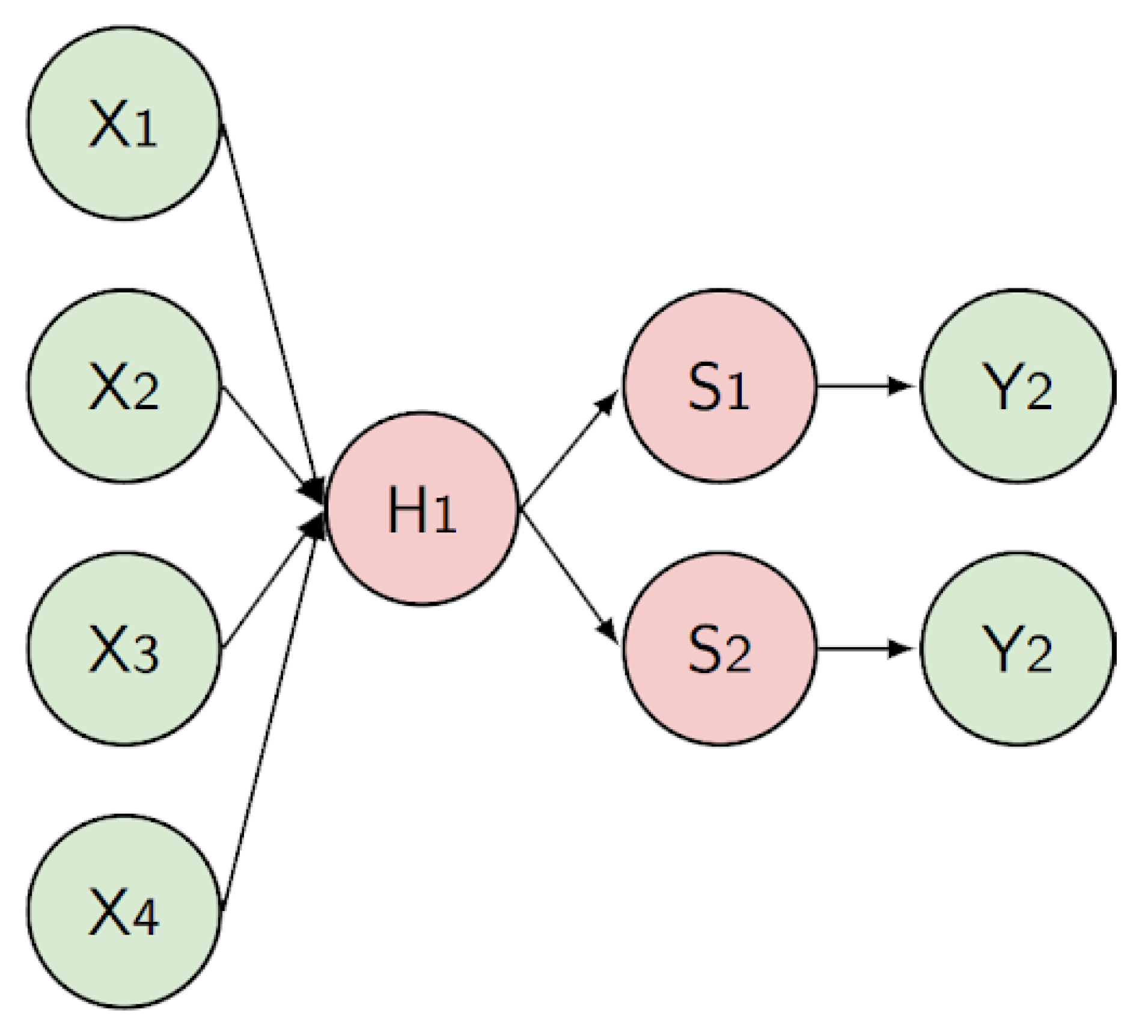
Figure 2.
The BM architecture of the mapped DNN.
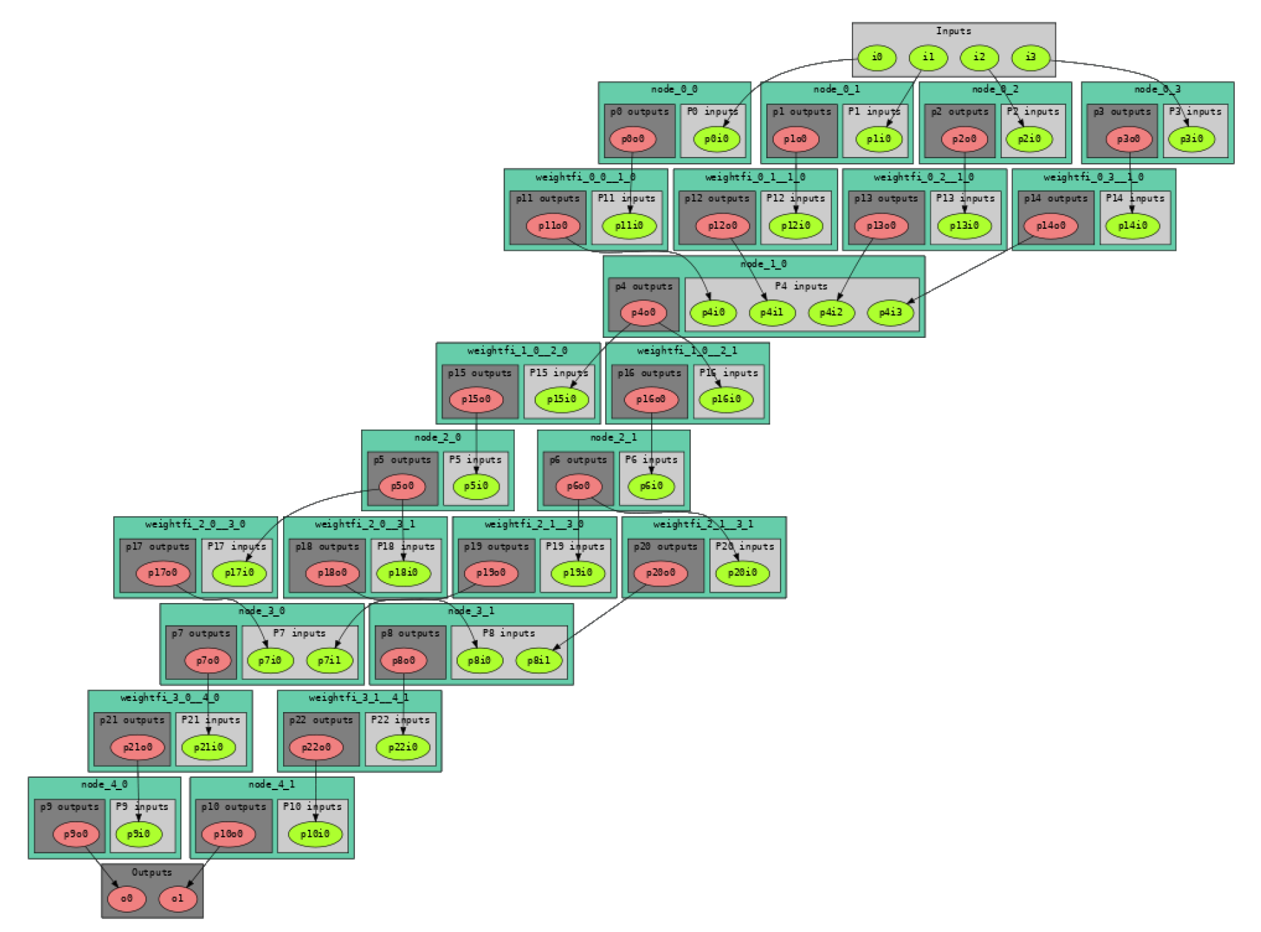
Figure 3.
DNN model used for the LHC jet tagging. The DNN graphical representation shows a fully connected NN with 16 input neurons, 3 hidden layers with 64, 32, 32 neurons and 5 output neurons.
Figure 3.
DNN model used for the LHC jet tagging. The DNN graphical representation shows a fully connected NN with 16 input neurons, 3 hidden layers with 64, 32, 32 neurons and 5 output neurons.
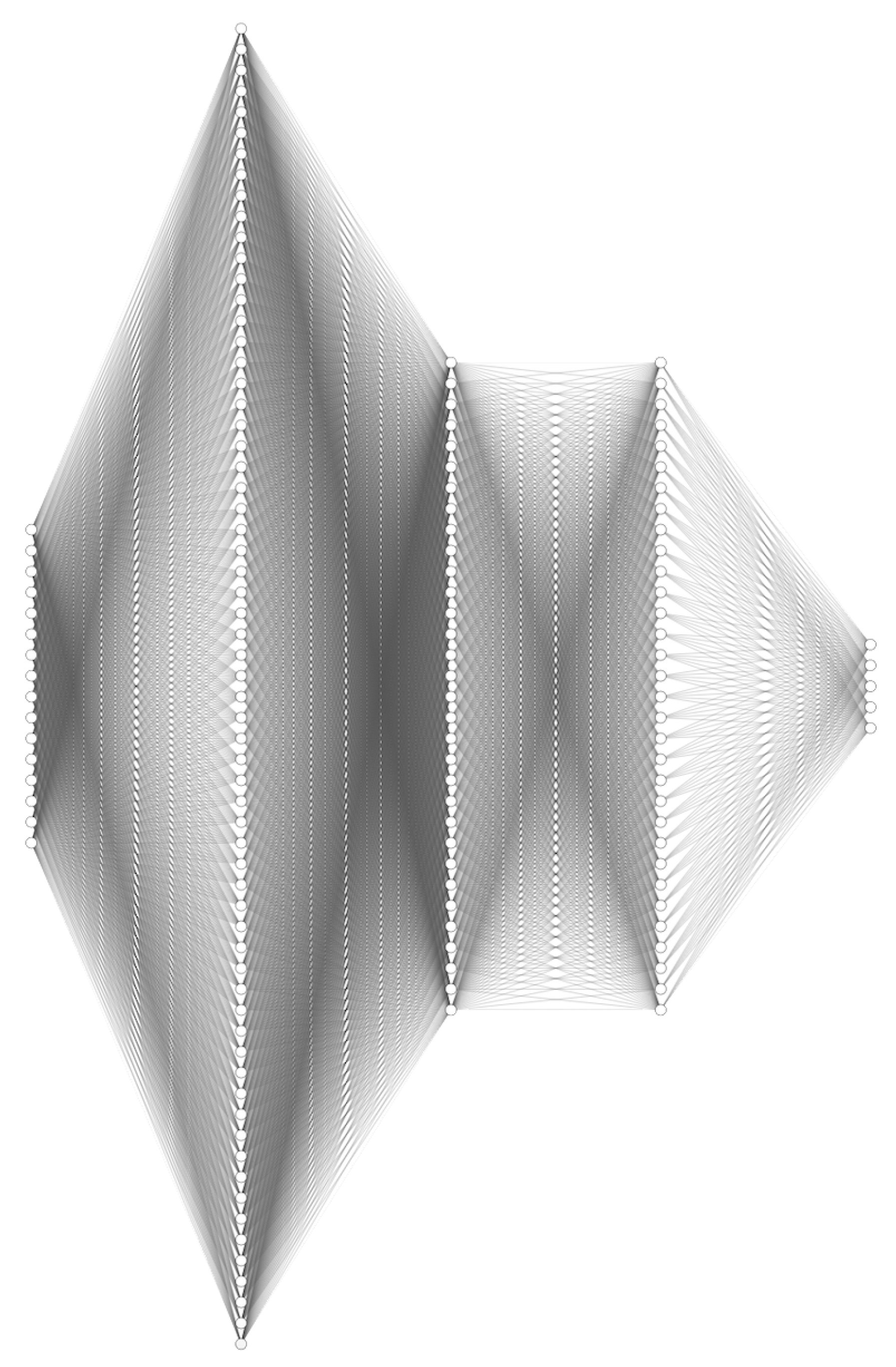
Table 1.
Numerical representations and corresponding prefixes used within the bmnumbers package
| Numerical representation | Prefix | Description |
|---|---|---|
| Binary | 0b | Binary number |
| Decimal | 0d | Decimal number |
| Hexadecimal | 0x | Hexadecimal number |
| Floating point 32 bits | 0f<32> | IEEE 754 single precision floating point number |
| Floating point 16 bits | 0f<16> | IEEE 754 half precision floating point number |
| Linear Quantization | 0lq<s,t> | Linear quantized number with size s and type t |
| FloPoCo | 0flp<e,f> | FloPoCo floating point number with exponent e and mantissa f |
| Fixed-point | 0fps<s,f> | Fixed-point number with s total bits and f fractional bits |
Table 2.
Comparison of the energy consumption of the ZedBoard BM with the ARM Cortex A9 and the Intel i7-1260P CPUs. The values are expressed in terms of their order of magnitude to highlight the relative differences in performance and energy efficiency across the systems. The System column indicates the system used for the inference, while the Time / Inf (s) and En. / Inf (J) columns show the time taken for a single inference (calculated from clock cycles, counted using the benchcore for the FPGA) and the energy consumption per inference (measured using the Perf tool for the CPUs).
| System | Time / Inf (s) | En. / Inf (J) |
|---|---|---|
| ARM Cortex A9 | ||
| Intel i7-1260P | ||
| ZedBoard BM |
Table 4.
The table presents the LUTs, REGs and DSPs used, along with their respective percentages, for the HLS4ML implementation using the AlveoU55C. It also includes the latency and accuracy.
Table 4.
The table presents the LUTs, REGs and DSPs used, along with their respective percentages, for the HLS4ML implementation using the AlveoU55C. It also includes the latency and accuracy.
| Data type | LUTs | Luts % | REGs | REGs % | DSPs | DSPs % | Latency ( ) | Acc % |
|---|---|---|---|---|---|---|---|---|
| fixed<16,6> | 134373 | 10.31 | 136113 | 6.89 | 255 | 2.83 | 0.17 ± 0.01 | 95.11 |
Disclaimer/Publisher’s Note: The statements, opinions and data contained in all publications are solely those of the individual author(s) and contributor(s) and not of MDPI and/or the editor(s). MDPI and/or the editor(s) disclaim responsibility for any injury to people or property resulting from any ideas, methods, instructions or products referred to in the content. |
© 2025 by the authors. Licensee MDPI, Basel, Switzerland. This article is an open access article distributed under the terms and conditions of the Creative Commons Attribution (CC BY) license (http://creativecommons.org/licenses/by/4.0/).
Copyright: This open access article is published under a Creative Commons CC BY 4.0 license, which permit the free download, distribution, and reuse, provided that the author and preprint are cited in any reuse.


