
Submitted:
26 May 2025
Posted:
27 May 2025
You are already at the latest version
Abstract
Hand gesture recognition is used in human-computer interaction, with multiple applications in assistive technologies, virtual reality, and smart systems. While vision-based methods are commonly employed, they are often computationally intensive, sensitive to environmental conditions, and raise privacy concerns. This work proposes a hardware/software co-optimized system for real-time hand gesture recognition using accelerometer data, designed for a portable, low-cost platform. A Convolutional Neural Network from TinyML is implemented on a Xilinx Zynq-7000 SoC-FPGA, utilizing fixed-point arithmetic to minimize computational complexity while maintaining classification accuracy. Additionally, combined architectural optimizations, including pipelining and loop unrolling, are applied to enhance processing efficiency. The final system achieves a 62× speedup over an unoptimized floating-point implementation while reducing power consumption, making it suitable for embedded and battery-powered applications.
Keywords:
SoC-FPGA
; pattern recognition
; convolution neural networks
; hardware/software co-design
; hardware accelerator
; high-level synthesis
1. Introduction
Hand gesture recognition has become an essential component of human-computer interaction, enabling touch-free control in applications such as assistive technologies, virtual reality, robotics, and smart home systems. Many existing gesture recognition systems rely on camera-based approaches, which, despite their effectiveness, present several challenges, including high computational complexity, sensitivity to environmental conditions, and privacy concerns. An alternative solution is the use of accelerometers, which offer a lightweight, low-power, and privacy-preserving method for capturing hand movements. However, the implementation of real-time gesture recognition on low-cost, portable hardware remains a significant challenge due to the limited computational resources and power constraints of embedded systems.
This work presents a hardware/software co-optimized system for real-time hand gesture recognition based on accelerometer data, implemented on a low-cost System-on-a-Chip Field-Programmable Gate Array (SoC-FPGA) from the Xilinx Zynq-7000 family. A SoC-FPGA integrates both processor and FPGA architectures into a single device, providing higher integration, lower power, smaller board size, and higher bandwidth communication between the processor and FPGA. While the CNN accelerator was implemented on the FPGA fabric, the CPU coordinates its operation.
Three hardware optimizations were done to reduce the execution time. The first optimization was the introduction of the pipeline, achieving an overall speedup of 26.7x. The secund optimization was the Loop Unroll technique, resulting in an overall speedup of 41.5x. Finally, some of the layers were merged and implemented as one function, which decreased the resources needed, while also achieving an overall speedup of 62x when compared to the unoptimized hardware architecture using floating-point representation.
2. Gesture Recognition with Convolutional Neural Networks
In this work, a gesture recognition system was used as an example of implementing a NN for gesture recognition from an accelerometer placed on a subject’s hand to detect gestures. This model can detect three different gestures. The model was trained using the TensorFlow Lite framework ([1]).
Figure 1.
Gestures supported by the proposed (from [2]).
Figure 1.
Gestures supported by the proposed (from [2]).
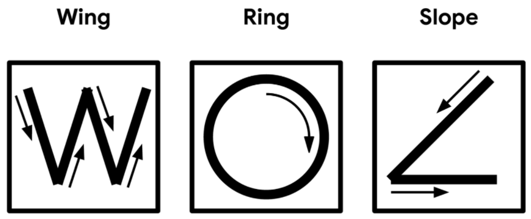
Figure 2 shows the overview of the gesture recognition model. The input of the NN model is the data from the accelerometer. The model has 7 layers, of which 2 of them are Convolution Layers.
All the layers of the model are represented in Table 1 below. The table also has the Input Shape of the Layer, in other words, the way the input data is organized. There are also the Output Shape of each layer and the Number of Parameters that each Layer needs so they can compute the output values, for example the kernels for the convolution layers.
Training data and the corresponding output are needed for each gesture to train and test the model. Each gesture was collected from 10 people and stored in 10 files, one file for each person. Each file has approximately 15 individual performances, there are also 10 files for the unknown gestures. The data was split so that 6 files are used for the training, 2 are used for validation, and another 2 for testing. The model was tested with an accuracy of 93,23% and a loss of 0,2888. These values are considered very good as it predicts the correct class with 93% of certainty.
The first layer is a convolution, it receives a set of input values directly from the accelerometer, and then does a convolution with those values. The input data has a shape of (128, 3, 1) which means that it is necessary 128 sets of accelerometer measurements for all the 3 axes (x, y and z). It has 8 kernels in the shape of 3x4, the output is 8 different matrices that capture different features of the input data. To do a convolution, first, it is necessary to know all the values of the kernels and biases that are stored in the network model.
Each convolution operation produces only one result, then, the kernel iterates through all the input values. Once the first kernel finishes all the convolution operations, the second kernel iterating through all the input values, until the last kernel finishes. This layer has output data in the shape of (128, 3, 8) and it needs 104 auxiliary parameters, 96 () for the 8 kernels plus 8 additional values for the offset of each kernel.
After the Convolution layer, a MaxPooling is done, this layer chooses the biggest values within a 3x3 matrix. The layer looks at 9 values at the same time and then shifts through all the data. In the end, it shrinks the data into the shape of (42, 1, 8), by removing redundant information while retaining the most significant features.
The second convolution is a 3D Convolution and has the shape of the input data as (42, 1, 8). There are 16 kernels which also have 3 dimensions (4, 1, 8). We have a 42x8 matrix as the input and a 4x8 kernel. Once again, the kernels shift through all the data, producing the output shape of (42, 1, 16). This layer needs 512 () parameters for all 16 kernels plus one bias for each kernel (16 in total), leading to 528 auxiliary parameters.
The second MaxPool is the same as the first one, the differences being the input and output shapes. The input has the shape (42, 1, 16), the MaxPool chooses the highest values from a set of 3 values (3x1 matrix), and it shifts through all the values for all 16 channels. In the end, the data has the shape (14, 1, 16).
The Flatten layer is used to reshape its input data into a single vector, and it "flattens" the values. In this case, it receives the output of the second MaxPool, in the shape of (14, 1, 16). It starts in the first dimension (first 14 values) then the second, and so on until it is all Flattened out (14 values each time), producing an output with the shape (224), notice that only maintains one dimension.
The Dense layer uses to all the values of the input independently, instead of a set of values. It multiplies all the input values by a weight given by a kernel and sums all the products into a single value. In other words, instead of having a small kernel that shifts through the data, the Dense layer has one big kernel that multiplies with all the input data at once. It can also have multiple kernels, in the case of the first Dense it has 16 kernels, so it repeats the operations 16 times with different weights (kernels), computing 16 different values, giving an output shape of (16). It needs 3584 () auxiliary values for all the weights of each one of the outputs, it also needs 16 extra values for the offset of each value reaching a total of 3600 parameters.
The second dense layer is exactly like the previous layer, but now it has 4 kernels with different weights, which means that it outputs 4 values, and the output is in the shape of (4). Once again, this layer needs auxiliary parameters, 64 (16x4) for each one of the 4 kernels plus the 4 bias values for each output, giving a total of 68 parameters. With the output values, a Softmax computation can be done, the outputs of the Softmax are the probabilities of our 3 gestures and 1 additional output for the unknown gestures, so the sum of all the values must be 1.
3. HW/SW Architecture for Gesture Recognition
4. Software Model Implementation in C
The Original TinyML Source implementation code uses a compiled library for the target MCU, thus it was impossible to identify which operations were being executed. The solution was to study and implement the layers of the model and get information about the parameters and make a new implementation from scratch to use the NN! model.
The first step was to create constants for all the parameters (kernels and bias), then create a variable for the input, and finally, start to do all the layers one by one and check in every step if the code is doing what it’s supposed to. Finally, after all the layers are done, it was necessary to create a function that reads a file, stores the input values in the correspondent variable, and starts going through all the layers to produce the output and repeat until the end of the file.
The source code flowchart is shown in Figure 3, where it is possible to see that the code has 3 actions, gather the input data, do the model inference and display the output.
Table 2 shows the errors between the code that was done in C language and the Original TinyML Code. There are some errors as expected derived from several causes. For example, the operations are slightly different from the Original TinyML Code, and the variables are different in one code when compared to another. This is because the compilers are different, the original TinyML code was compiled in a Linux subsystem with GCC 9.4.0 compiler, while the custom code was compiled in Windows with MinGW-W64-builds-4.3.5 compiler. All of that reasons can cause differences in the output of the model but, as we can see in the table, the errors are too small and all the predictions stayed the same throughout all the test files.
Figure 4 shows the dataflow of the model. So, at the end of each layer, the outputs are stored in memory and the next layer loads these values to start executing.
5. Floating-Point vs Fixed-Point Representations
The initial C description of the CNN model in Vitis HLS had the data variables in Floating-Point representation. However, to have better execution time and simpler hardware blocks (such as multipliers and adders), the Floating-Point representation was converted into a Fixed-Point representation. The downside of this representation is that has a limited range and less precision than the Floating-Point, which may result in output errors. Therefore, a study was performed, where the number of bits required for the Fixed-Point representation was evaluated. This study helped to understand the tradeoff between resources needed and the network model accuracy. If fewer bits are used, the resources needed are reduced but the network model accuracy also decreases.
5.1. Floating-Point
The first implementation in Vitis HLS used Floating-Point variables. In IEEE Standard for Floating-Point Arithmetic representation [3] (32 bits), there is no set number of bits for the integer part nor the decimal part. Instead, there is 1 bit for the sign, 8 bits for the exponent, and 23 bits for the mantissa.
When comparing to Fixed-Point representation, the operations with Floating-Point representation are much more complex and time-consuming. The adders take about three clock cycles, and the multipliers take about six clock cycles.
The code was simulated in Vitis HLS, with Zynq-7020 SoC-FPGA as the target device. After running the code through all the inputs of the provided files, all the predictions matched the predictions of the original TinyML code, however, some differences were presented in the output values. Table 3 presents the Errors between the output of the original TinyML code and the Vitis HLS code using Floating-Point representation. These errors are not that significant, because the minimum value for a gesture to be chosen is 0.25 (because there are 4 gestures and the sum of all the values must be 1) which is 100,000x higher compared to the Maximum Absolute Error (MAE), which is about 2.22E-06.
Note that these errors are different from the C code from CLion, despite the operations being the same and the overall code very similar. The reason for the existence of these differences is that the compilers used are different from each other. In the CLion IDE, the compiler that was used is MinGW-W64-builds-4.3.5. Vitis HLS has GCC as a compiler, this implies that the operations are done differently which results in slightly different outputs. To prove that, the same code that was on CLion, was compiled with GCC using an Ubuntu subsystem for Windows, on that test, the outputs were the same as the Vitis HLS.
5.2. Fixed-Point
Fixed-Point adders only take one clock cycle and multipliers take one to two clock cycles, which is less than Floating-Point operators. Moreover, the resources required to implement the operators in Fixed-Point are also reduced.
In Fixed-Point representation, there are bits set to the integer part and bits set to the decimal part, so for instance, if a number has 8 bits in the format Q4.4, this means that it has 4 bits to represent the integer part and 4 bits to represent the decimal part. This representation is better than the Floating-Point representation for this work. However, there are some downsides, like the loss of precision when compared with the Floating-Point representation. The advantages are that with the Fixed-Point all the operators are simpler to implement. Therefore, the complexity is smaller than the Floating-Point, while the computing time is faster. Also, by reducing the complexity, Fixed-Point needs fewer resources to implement when compared to Floating-Point. So, as long as the values are not too different during the computations of the algorithm,or the error is acceptable, this option is much better than Floating-Point.
So, for instance, if we want to represent a number with 8 bits with 3 bits for the integer part and 5 bits for the decimal part, then the initialization needs to be "ap_fixed<8, 3 > var;". Therefore when initializing a Fixed-Point variable, it is necessary to provide two arguments (W and I), while the other arguments are optional and have default values.
The W and I arguments are 36 and 17 respectively, which means that the variables have 36 bits with 17 bits for the integer part and 19 bits for the decimal part. However, the number of bits can be decreased, more in Section 7.1. To avoid Overflows in this work, there were provided enough bits for the integer part, hence the Q argument is the only optional argument that needs concern. By consulting the User Guide [4], seven options were withdrawn for this argument:
- RND: Round to plus infinity.
- RND_ZERO: Round to zero.
- RND_MIN_INF: Round to minus infinity.
- RND_INF: Round to infinity.
- RND_CONV: Convergent rounding.
- TRN: Truncation to minus infinity (default).
- TRN_ZERO: Truncation to zero.
Out of these 7 options, 4 were chosen to be evaluated: TRN; TRN_ZERO; RND_ZERO; RND_CONV. In this evaluation the first kernel is initialized with the different quantization modes, these values are then compared with the Floating-Point values of the kernel.
The results of using different Quantization Modes are shown in Table 4. It can be concluded from the table, that the best modes are RND_ZERO and RND_CONV, which have smaller errors in every metric. Both of them have the same errors because both modes try to round the value to the nearest integer, the problem comes when the number is in the middle of two integers, for example, 5.5 is in the middle of 5 and 6.
To choose the best mode for this work, another evaluation was done. We evaluate how many resources were needed to do a simple operation for each of the 4 modes.
Looking at Table 5 it is possible to conclude that the default mode (TRN) is the one that consumes fewer resources, on the other hand, both RND_ZERO and RND_CONV are the ones that consume the most, with a small increase over TRN_ZERO. The two modes consume the same resources used as well as generate the same errors. The conclusion is that both are suitable to use, in this work the one that was chosen was convergent rounding (RND_CONV).
Following the choice of the quantization mode, a random input was chosen from the test files. This input goes through all the layers of the model, and all the variables that were in Floating-Point are now in Fixed-Point with the chosen quantization mode. The output of each layer was compared with the Floating-Point code, in Table 6.
Since the intermediate values (output values of each layer) are mostly big integer numbers (bigger than 100), the errors presented in the table compared to those numbers are very small. In all of these evaluations, the Fixed-Point variables had 36 bits with 17 bits for the integer part and 19 for the decimal part. Further analysis of the number of bits required for the integer and decimal parts is done in Section 7.1.
6. Digital System Design Optimizations
6.1. Pipelining
When scheduling without pipeline the next instruction only begins when the previous instruction is finished, but with pipeline that is not the case. Because the instructions are independent, it is possible to start the next instruction without the current one finishing, utilizing the available resources that are not being used.
Without pipeline all the operations of each layer were being done sequentially, producing one output only when the previous one had finished.
Initially, the first convolution layer would load every value that was necessary for the convolution, that is, all the values of the kernel and all the input values needed. These loads were executed every iteration, which means that it would do 18 to 24 loads for each output, storing this output in the end. The cause of this violation was the number of ports, there weren’t enough ports for all the necessary loads and stores. This means that there were not enough resources to pipeline this loop. The solution is to reformulate the code, so the number of loads and stores decreases. First, the number of main loops was reduced, from one outer loop and two inner loops to one main outer loop.
In the convolution layer, the kernel moves through the input data, as shown in Figure ??, and goes through the same values as before, so the code can reuse those values. It only needs to have a 3x4 matrix with the values that the kernel at that moment and load a new value per iteration. This is a way to reduce the number of loads per iteration. Before there were either 20 or 24 loads only in one iteration (12 for the kernel and 10 to 12 for the input data), now the input data only needs one load per iteration and the kernel none because it is the same for all the input data. The only time this doesn’t happen is in the beginning because it’s necessary to load at least 11 values of the input data and all the 12 values of the kernel, and when the kernel changes, it is necessary to load all the 12 values again for the new kernel.
There are some precautions to be taken, as the user guide says "Arrays are typically implemented as a memory (RAM, ROM or FIFO) after synthesis." [4]. Therefore, the code can’t just load an input value, for instance, just to store in another memory so, to solve this problem.
Without pipeline, this new architecture is slower than the previous one, when synthesized. Now with pipeline, the synthesis led to another error. This time it was a Timing Violation, the clock cycle was 10ns, but the critical path was slower than the clock cycle. The fix was simple, just slow the clock a bit, from 10 ns to 10.4 ns. In the end, even with the fact that the clock cycle was slower, there were improvements in the speed, but the resource usage increased as well.
Advancing to the second Convolution, the same steps were done and, although the number of loads per iteration after the optimization was 8, Vitis HLS was able to pipeline the loop, increasing the resources used as well as the speed. This optimization was done on all layers of the model, enabling the use of pipeline in every layer. The clock had to be changed yet again from 10.40 ns to 10.41 ns when optimizing the 1st Dense due to a Timing Violation. In the end, the speedup achieved was 26.7x when compared with the code without pipeline with a 10 ns clock cycle.
6.2. Loop Unroll
Loop Unroll (LU) is a known optimization in which, instead of the loop doing one iteration at a time, it does several iterations in parallel. This optimization tries to increase the execution speed while increasing the resources used in return, it is a space-time trade-off.
Starting with the 1st Dense layer, in this function, there are three loops, the outer loop that shifts through the kernels and two inner loops to shift through all the data. By unrolling the most inner loop, it was possible to increase the speed, as wished (11.1x function speedup). The problem was when the inner loop of the 2nd Dense was unrolled, this time the speed got worse. There could many many causes for this problem, in this layer, there are many loads and stores, when the loop is unrolled, it tries to do all the loads inside the loop, and all of these loads are followed by a store and a load that are outside the loop.
When a loop is unrolled, there’s a possibility that there are not enough ports to load and store all the necessary values, and the circuit needs to stall and wait before it can load the value. This will limit the performance by suspending the execution of the computations in the pipeline, impacting the throughput and latency.
However with the pipeline, the clock cycle had to be changed because of the critical path in the 1st Convolution, and after that in the 1st Dense, when the Loop Unroll was performed in the Convolution, even though the execution time stayed the same, the critical path decreased. Now the clock cycle can be faster, changing from 10.41ns to 10.37ns (1.004x overall speedup). In the end, after both, the Pipeline and the Loop Unroll optimizations, the speedup achieved was 41.5x.
6.3. Merging
After observing the Schedule Viewer tool in Vitis HLS, it was detected that a function/layer only starts its execution when the previous one finishes. Some layers don’t need all the input values to begin their execution, instead, they can start the execution with some of the inputs, and while it’s doing the operations with that values, the remaining input values arrive from the previous layer. This way, it is possible to parallelize even more the overall execution of the architecture, increasing its speed.
The method to implement this in Vitis HLS is, instead of having independent functions, those functions can merge and code that new function in a way that the next layer starts before the previous finishes. Starting with the 1st Convolution and the 1st MaxPool, this is a simple case, basically in the Convolution function, instead of storing each output value, this value just needs to be compared to the current maximum value, if the output value is greater, then update the maximum value with the current output value. After 12 values are compared, an output value is produced and stored (output of the MaxPool), and the maximum value is reset to 0. Therefore, instead of the MaxPool waiting for the Convolution to produce all the output values before starting to execute, both can be executed at the same time (1.325x function speedup).
The 2nd Convolution and the 2nd MaxPool can also merge. The same method used in the merging of the 1st Convolution was done, increasing the execution speed (1.937x function speedup). Now it is time to see if there is a possibility to merge more layers to speed up the execution.
In the case of merging the 1st MaxPool with the 2nd Convolution, the speedup obtained was less than 1.05x, this is because the MaxPool computes all the outputs of one kernel consecutively, and then computes the values for the next kernel, and so on. Meanwhile, the 2nd Convolution needs input values from all the kernels to compute any of the output values. So, even if it was merged, the 2nd Convolution has to wait almost until the end to start the computation, furthermore, the complexity of the code would increase drastically. Concluding, the merge of these two layers didn’t happen because it would end up with too much work for a small reward. The same happens with the 1st Dense and the 2nd Dense because the 2nd Dense needs all the output values of the 1st Dense before it can start computing, achieving little to no speedup.
Finally, merging the 2nd MaxPool with the 1st Dense. Contrary to what happens with the 2nd Dense, this time it is possible to change the architecture to achieve a greater speedup. Even if the Dense needs all the values to start computing, it is possible to have only the intermediate variables. These variables store the intermediate values of the output values, this means that every time the MaxPool produces an output, these variables are updated with a new intermediate value. In the end, the outputs are produced all at the same time, and the speed has an increase (1.427x function speedup). The Merging finishes all the optimizations that were implemented, in the end, the speedup of all these optimizations is 61.978x.
7. Evaluation of the Proposed System
7.1. Classification Accuracy
The architecture was evaluated for a different wordlengths for each variable. In this evaluation, the output values of the architecture before any optimization, are compared with the original output values from a gesture recognition system. The data used is the same used for testing the gesture recognition model, which had a 97,43% accuracy. The code used for this evaluation was the one after the Fixed-Point was implemented before any of the optimizations.
The goal is to try to reduce resource utilization without having an accuracy decrease. It is expected however an increase in the errors when reducing the number of bits
The Fixed-Point variables were divided into eight groups:
- Parameters: This group contains all the parameters of every kernel and bias values for all layers (4300 values stored).
- Input: This group contains the input values (384 values stored).
- 1st Convolution: This group contains the output values of the 1st Convolution (3072 values stored).
- 1st MaxPool: This group contains the output values of the 1st MaxPool (336 values stored).
- 2nd Convolution: This group contains the output values of the 2nd Convolution (672 values stored).
- 2nd MaxPool: This group contains the output values of the 2nd MaxPool (224 values stored).
- 1st Dense: This group contains the output values of the 1st Dense (16 values stored).
- 2nd Dense: This group contains the output values of the 2nd Dense (4 values stored).
The idea is to reduce the wordlength as much as possible while affecting the accuracy as little as possible, this way it is possible to reduce the FPGA resources that are being used (less memory is needed to store the values). In the beginning, all the variables had 36 bits (17 for the integer part), so the initial strategy was to reduce the bits group by group without having errors between the output values and the original output errors.
The Table 7 shows how many bits were used in each variable group for the different tests, note that the first number is the total wordlength, followed by the bits for the integer part and ending with the bits for the decimal part.
By observing the output errors for each test on Table 8, it is possible to notice that the errors increase with each test, while the wordlength decreases. There are also some curious facts, for example in T3, there is one Mismatch Prediction (the predicted gesture is not the same as the original prediction), however, the original prediction is wrong, instead of an unknown gesture, the correct prediction is ”O” gesture, which was the prediction in T3. So, the accuracy in T3 has a slight improvement (about 0.14%). Also, the one missed prediction in T3, disappears in T4, going back to 0 Mismatch Predictions. Finally, T5 has 7 Mismatch Predictions, most of them were the right prediction in the original project, only 2 being the right prediction in T5 and 1 being wrong in both models.
Table 9 shows how the resources decrease for the tests with smaller bit variables. Even if the errors and the mismatch predictions increase, the resources used decrease, so the area used decreases as well. The T0 test in the table corresponds to a test done with all the variables with 36 bits (17 for the integer part), before any change. These values lead to the graph shown in Figure 5, where it is possible to see the error increase while the number of FFs decrease.
A new strategy was implemented, this time each group would be tested independently, that is, in each test, only one group would change the wordlength, while all others would have 36 bits (17 for the integer part). This way, it is possible to study what layers have more impact on the outputs and accuracy. Firstly the wordlength for the integer part was reduced as much as possible without having any overflow, then the wordlength for the decimal part was reduced one by one until there were 0 bits for the decimal part. However, the Parameters group was a bit different, this is because it is mostly composed of small numbers with a big decimal part, the integer part needs only 3 bits while the decimal part needs more bits. The threshold used for this particular group was that the percentage of mismatch predictions (differences between the tests predictions and the original predictions) has to be lower than 5%. For the Parameters group, when the number of bits of the decimal part is 9 bits, there are 65 mismatch predictions out of 729 predictions, this gives a percentage of 8.92%, exceeding the threshold.
Table 10 shows the number of mismatch predictions depending on the number representation, the number of bits inside the parenthesis is the number of bits for the integer part, and these bits never change. For instance, "1st Dense (14)" means that the 1st Dense group always has 14 bits for the integer part for this study. Also, it is possible to see that when the number of bits decreases, the number of mismatch predictions increases, although there are a few exceptions.
With the information from Table 10, new tests were done, this time the goal was to decrease the number of bits as much as possible for the groups that have more values to be stored, to decrease the memory resources as much as possible. In other words, the critical groups to be reduced are the Parameters, the 1st Convolution + 1st MaxPool, and the 2nd Convolution + 2nd MaxPool. Table 11 has the number of bits for each group for the new tests (T6 and T7) as well as the previous test T5, it is possible to see that it is impossible to reduce the number of bits for all the Convolution and MaxPool groups without generating any overflow since the limit was already reached (reducing the number of bits of the integer part would generate overflows). The only critical group left to change is the Parameters group, which is the only group that changed between T6 and T7.
From Table 12 it is possible to extract a clear improvement from T5 to T6, not only did the errors decrease (Mean Absolute Error, Quadratic Error, and Standard Deviation) but the mismatch predictions and the number of bits stored decreased as well. From T6 to T7 there’s a tradeoff between reducing the number of bits while increasing the errors as well as the number of mismatch predictions. No further tests were done because, if the number of bits of the Parameters decreased any further, the number of mismatch predictions would drastically increase, exceeding the threshold of 5%. Also, there isn’t an advantage in reducing the number of bits for the dense groups because the number of bits stored would only have a slight decrease. The number of mismatch predictions can be even worse with real data, this is because the input data used, was the one used for training, validation, and testing of the model, which means that the model can be overfitted for these tests, which can decrease the accuracy even further.
As expected, the number of resources decreases when the number of bits decreases, Table 13 shows how many resources were used, confirming this reduction. This concludes the accuracy test, showing that it is possible to have a reduction in resources without heavily reducing the accuracy of the model.
7.2. Impact of Design Optimizations
The final architecture combines all the optimizations done, as well as the T7 test. This means that this architecture has pipeline implementation, loop unrolls and the merge of some layers, and also has a reduced number of bits to store the variables. The output values of this architecture were compared with the original output values, in Table 14.
Comparing these errors with the errors of the T7 test, the final architecture has a slight improvement, having a decrease in Mean Absolute Error, Quadratic Error, and Standard Deviation. This decrease can be explained by the merge optimization because this optimization changed the architecture to do multiple layers before it stores the output in the memory. This architecture change comes with a difference in the way the variables are stored and the operations are done.
7.3. FPGA Resources
This section compares the differences in the FPGA Resources used for the work in different Design Solutions (DS). The chosen DS were the following:
- Design Solution 1: This DS is after the Fixed-Point is implemented, before the Pipeline optimization.
- Design Solution 2: This DS is after the Pipeline optimization is implemented, before the Loop Unroll optimization.
- Design Solution 3: This DS is after the Loop Unroll optimization is implemented, before the Merge optimization.
- Design Solution 4: This DS is after the Merge optimization is implemented.
- Design Solution 5: This DS is the final architecture with bit-width optimization (Section 7.2).
In all DS, except for DS 5, the number of bits stayed the same, with all Fixed-Point variables having 36 bits with 17 for the integer part. The number of resources used in all DS’s presented in Table 15.
It can be observed a growth in resources from DS 1 to DS 2 as expected because when the Pipeline is implemented, different stages of the architecture are executing at the same time, this means that more resources are necessary to do all those tasks at the same time, increasing the execution speed. There is another increase in resources from DS 2 to DS 3, this time was when the Loop Unroll was implemented, well the LU unrolls the loop, executing some iterations in parallel, instead of doing one iteration after another sequentially. Since there are more tasks to be done in parallel, it is necessary more resources to do those tasks. In DS 4, most of the resources decreases, because in DS 4 some layers were merged. Meaning that some of the resources that weren’t being fully used before can now be used for both layers at the same time, sharing this way the resources, instead of each one having their resources. Also, with this optimization, there’s no need to transfer data from some layers to others, since those layers are merged. DS 5 is the DS with fewer resources used after DS 1, this was expected since in DS 5 the number of bits to store the variables was reduced, reducing this way the resources needed.
The available resources for Zynq-7020 SoC-FPGA are shown in Table 16. Comparing these resources with the ones from Table 15, there are only two Design Solutions that could potentially be configured into the FPGA because DS 2, 3, and 4 all need more DSPs than the ones available in the FPGA. DS 3 is the worst in terms of resources required since it exceeds both DSPs, FFs, and LUTs of the Zynq-7020 SoC-FPGA. In terms of BRAM, the FPGA has enough blocks for all Design Solutions.
Concluding, there are some optimizations that, even though they speed up the execution time, also increase the required resources which can exceed the available resources. Other optimizations can help in both parameters, increasing the execution speed while decreasing the resources used. DS 5 has a resource reduction when compared to the previous DS while maintaining its execution speed, but decreasing the model accuracy.
7.4. System Performance
This section talks about the differences in the System Performance, that is, how much time it is necessary to execute the inference. These comparisons have two control groups after the implementation of the Fixed-Point when the code hasn’t suffered any optimization change yet. One of the control groups has a clock with 10ns while the other has a clock with 10.4ns. Then, those two control groups are compared to every step of the optimizations that were done.
Table 18 has the Speedup Performance for the Pipeline optimization. It is divided into functions (or layers) each one being pipelined sequentially, and not independently, that is, when for example the 1st Convolution is pipelined, it stays pipelined until the end. By observing this data, it is possible to see that the Convolution layers had a speedup, the 1st having a speedup of 42.3x and the 2nd having a speedup of 123.4x. But the total speedup isn’t as big as the function speedup, in fact, it almost doubled the speed in the 1st Convolution and it has a 5.5x speedup in the 2nd Convolution. After the Pipeline optimization, the total speedup is 26.7x, which is almost 5x less than some function optimizations.
Table 19 and Table 20 have the Speedup Performance for the remaining optimizations, as well as the speedup after the Pipeline optimization for reference.
These optimizations are lower compared to the pipeline ones. Once again, the reason is Amdahl’s law. In this case, the tasks can be divided into parts that can be parallelized and parts that cannot. For example, we cannot do the 2nd Dense while the 1st Dense is still computing, because the 2nd Dense needs all the outputs of the 1st Dense to start its computation. With the pipeline optimization, the parts that can be parallelized were already optimized, which means that the time fraction used by those parts decreased, leading to a lower speedup of the overall task. However, there were also some large speedups, for example, the Loop Unroll on the 1st Dense having a speedup of 11.1x. Besides, if the function speedups are minimal, the overall speedup is greatly increased, this is because it is always compared with the hardware architecture where the Pipeline was not yet implemented. Speedup after the Pipeline optimization reached at least 20x, even if a function speedup is small (for example 1.3x), the overall speedup compared to that control group shows an increase. For example, after the pipeline, the overall speedup is 26.7x, so if a new optimization has a speedup of 1.5x when combining these two optimizations, the overall speedup is 40.05x ().
The Final Architecture has an execution time of 4.250E+04 ns, a slight improvement compared to the execution time of the architecture after all optimizations (4.266E+04 ns), with a speedup of 1.003x. The Final Architecture’s overall speedup reach 62.21x when compared to the control group with the 10 ns clock. This improvement is a consequence of the number of bits being reduced, with fewer bits the operations are faster. For example, it is faster to do a 16-bit multiplication instead of a 32-bit multiplication, which results in a decrease in the overall execution time.
8. Related Works
Previous works on hand gesture recognition using Convolution Neural Network (CNNs) and Tiny Machine Learning (TinyML) have been identified and compared in terms of their target target devices, achieved performance, and FPGA resource utilization.
[5] FPGA-based Implementation of a Dynamic Hand Gesture Recognition System Target Device: Xilinx Zynq-7000 FPGA Achieved Performance: The system integrates hand tracking and gesture recognition components, utilizing a CNN for classification. The design emphasizes efficient resource utilization to achieve real-time performance. FPGA Resources: Specific resource utilization details are not provided in the available summary. [6] Low Power Embedded Gesture Recognition Using Novel Short-Range Radar Sensors Target Device: Not FPGA-based; utilizes short-range radar sensors Achieved Performance: The system employs a combination of CNN and Temporal Convolutional Network (TCN) models, achieving up to 92% accuracy across 11 challenging hand gestures performed by 26 individuals. FPGA Resources: Not applicable
[7] FPGA-based Implementation of Hand Gesture Recognition Using Convolutional Neural Network Target Device: Xilinx ZCU102 FPGA Achieved Performance: The system utilizes a CNN model trained using the Caffe framework, with bilinear interpolation applied to adjust image sizes. The implementation leverages FPGA parallelism to enhance processing speed. FPGA Resources: Specific resource utilization details are not provided in the available summary. DOI: 10.1109/ICIEA.2018.8397882
[8] Implementation of Tiny Machine Learning Models on Arduino 33 BLE for Gesture and Speech Recognition Applications Target Device: Arduino Nano 33 BLE Achieved Performance: For hand gesture recognition, a TinyML model was trained and deployed on the device equipped with a 6-axis Inertial Measurement Unit (IMU), enabling detection of hand movement directions. FPGA Resources: Not applicable DOI: Not available [9] A Real-Time Gesture Recognition System with FPGA Acceleration Target Device: Xilinx ZCU104 FPGA Achieved Performance: The system utilizes a modified version of ZynqNet to classify the Swedish manual alphabet (fingerspelling). Data augmentation and transfer learning techniques were employed to enhance model performance. FPGA Resources: Specific resource utilization details are not provided in the available summary. DOI: 10.1109/ICIP.2019.8803096 [10] Real-Time Implementation of Tiny Machine Learning Models for Hand Motion Recognition Target Device: Not FPGA-based; utilizes IMU sensors Achieved Performance: A CNN model was employed for hand motion classification, facilitating applications in human-computer interaction and sign language interpretation. FPGA Resources: Not applicable DOI: Not available [11] Real-Time Vision-Based Static Hand Gesture Recognition on FPGA Target Device: Xilinx Virtex-7 FPGA Achieved Performance: The system comprises modules for image acquisition, preprocessing, feature extraction, and classification, achieving efficient performance on FPGA platforms. FPGA Resources: Specific resource utilization details are not provided in the available summary. DOI: 10.1109/ACCESS.2018.2817560 [12] Hand Gesture Recognition Using TinyML on OpenMV Target Device: OpenMV Microcontroller Achieved Performance: The system leverages a CNN model to process image data, demonstrating the capability of microcontrollers to perform real-time image classification tasks. FPGA Resources: Not applicable DOI: Not available
Table 21 summarizes the performance of the related work from the state-of-the-art.
From the results it is possible to conclude that CNN models implemented on FPGAs generally achieve 75-90% accuracy, with real-time processing speeds ranging from 15 to 60 FPS. TinyML implementations, although more resource-efficient, typically offer accuracy between 75% and 82%.
In terms of FPGA resource usage, the Xilinx Zynq-7000 and ZCU102/ZCU104 SoCs were commonly used, with FPGA resource utilization in the range of 60-75% LUTs and 60-96 DSPs. More complex CNN architectures (ResNet-like, ZynqNet) require more DSPs and BRAM for efficient computation.
Regarding the optimizations applied some works using loop unrolling, fixed-point quantization, and pipelining saw significant improvements in performance. In general, FPGA-based implementations benefited from parallel processing, allowing faster execution than CPU-based or microcontroller-based TinyML implementations.
TinyML solutions, while more power-efficient and suitable for edge AI applications, generally performed slower and with lower accuracy compared to FPGA-based solutions. FPGA-based implementations showed superior real-time performance, but required more complex hardware and optimization efforts.
9. Discussion
The goal was to have a NN! implemented in a Soc-FPGA, without losing much accuracy compared to the same CNN model on a computer while trying to have a real-time classification (and hopefully have some speedup). This way, a computer is not needed to compute the classification, and it is possible to have the classification in a portable device, smaller and less power-hungry than a computer.
To reduce the resources needed, the number of bits of the Fixed-Point variables is also reduced, the tradeoff being a slight decrease in accuracy as shown in Section 7.1. If there are enough resources, it is also possible to implement some optimizations, increasing this way the execution speed. This means that, depending on the FPGA used, it may be necessary to reduce accuracy and speed, in order not to exceed the available resources. On the other hand, if there are enough resources, then it is possible to maintain the accuracy of the model while, possibly, increasing the speed of the classification, when compared to the computer.
10. Conclusions
In this work, all the simulations and synthesis in Vitis HLS target the Zynq-7020 SoC-FPGA. After all the evaluations of this device, the resources available were enough to implement the final hardware of this project. This means that there is no need to reduce the number of bits any further in the Fixed-Point variables and it is possible to implement all the presented optimizations since the overall FPGA utilization is 32% BRAM blocks, 48% DSPs, 16% FFs, and 43% LUTs.
This work showed that, by carrying out some hardware optimizations techniques and using Fixed-Point representation with enough bits to maintain high accuracy, we were able to implement a CNN for gesture identification in a portable and cheap device (like an FPGA) with the same accuracy as the original model and with real-time classification. The original TinyML code had an execution time of 113 (on Windows 10 laptop, Intel i7-11370H, 16Gb of memory), while in the Vitis HLS simulation (Zynq-7020 SoC-FPGA), the proposed architecture has an execution time of 42.66 , resulting in a speedup of 2.65x.
In future work, an interface could be done to read the values from an accelerometer, also this input data needs to be processed and provided to the FPGA to start the inference. Another interesting research study that could be done is to measure and analyze the energy consumption for different design solutions of this work to evaluate how the energy consumption varies in function of the used resources and execution time. This work could also be adapted to create a game, for example, that uses the gestures done to execute actions in the game, or use the gesture classification to control a device, according to the gesture that was done.
Funding
This research was funded by FCT grant number 2023.15325.PEX and the research project with reference IPL/IDI&CA2024/CSAT-OBC_ISEL, financed by the 9th edition of IDI&CA.
References
- Tensorflow. TensorFlow Lite. https://www.tensorflow.org/lite/guide, 2022.
- Daniel Situnayake, P.W. , TinyML; O’Reilly Media, 2019; chapter 11, 12.
- IEEE Standard for Floating-Point Arithmetic. IEEE Std 754-2008 2008, pp. 1–70. [CrossRef]
- Xilinx. Vitis High-Level Synthesis User Guide (UG1399). https://docs.xilinx.com/r/2021.1-English/ug1399-vitis-hls, 2021.
- Tsai, Y.C.; Lai, Y.H.; Xu, C.H.; Ruan, S.J. FPGA-based implementation of a dynamic hand gesture recognition system. In Proceedings of the IET International Conference on Engineering Technologies and Applications (ICETA 2023); 2023; 2023, pp. 41–42. [Google Scholar] [CrossRef]
- Eggimann, M.; Erb, J.; Mayer, P.; Magno, M.; Benini, L. Low Power Embedded Gesture Recognition Using Novel Short-Range Radar Sensors. In Proceedings of the 2019 IEEE SENSORS; 2019; pp. 1–4. [Google Scholar] [CrossRef]
- Zhang, T.; Zhou, W.; Jiang, X.; Liu, Y. FPGA-based Implementation of Hand Gesture Recognition Using Convolutional Neural Network. In Proceedings of the 2018 IEEE International Conference on Cyborg and Bionic Systems (CBS); 2018; pp. 133–138. [Google Scholar] [CrossRef]
- V, V.; C, R.A.; Prasanna, R.; Kakarla, P.C.; PJ, V.S.; Mohan, N. Implementation Of Tiny Machine Learning Models On Arduino 33 BLE For Gesture And Speech Recognition, 2022, [arXiv:eess.AS/2207.12866]. 2022; arXiv:eess.AS/2207.12866]. [Google Scholar]
- Núñez-Prieto, R.; Gómez, P.C.; Liu, L. A Real-Time Gesture Recognition System with FPGA Accelerated ZynqNet Classification. In Proceedings of the 2019 IEEE Nordic Circuits and Systems Conference (NORCAS): NORCHIP and International Symposium of System-on-Chip (SoC); 2019; pp. 1–6. [Google Scholar] [CrossRef]
- Khalife, R.; Mrad, R.; Dabbous, A.; Ibrahim, A. Real-Time Implementation of Tiny Machine Learning Models for Hand Motion Classification. In Proceedings of the Applications in Electronics Pervading Industry, Environment and Society; Bellotti, F.; Grammatikakis, M.D.; Mansour, A.; Ruo Roch, M.; Seepold, R.; Solanas, A.; Berta, R., Eds., Cham; 2024; pp. 487–492. [Google Scholar]
- Zhou, W.; Lyu, C.; Jiang, X.; Li, P.; Chen, H.; Liu, Y.H. Real-time implementation of vision-based unmarked static hand gesture recognition with neural networks based on FPGAs. In Proceedings of the 2017 IEEE International Conference on Robotics and Biomimetics (ROBIO); 2017; pp. 1026–1031. [Google Scholar] [CrossRef]
- Raza, W. Hand Gesture Recognition Using TinyML on OpenMV, 2023. (Date last accessed 03-March-2025).
Figure 2.
Overview of the gesture recognition NN model.
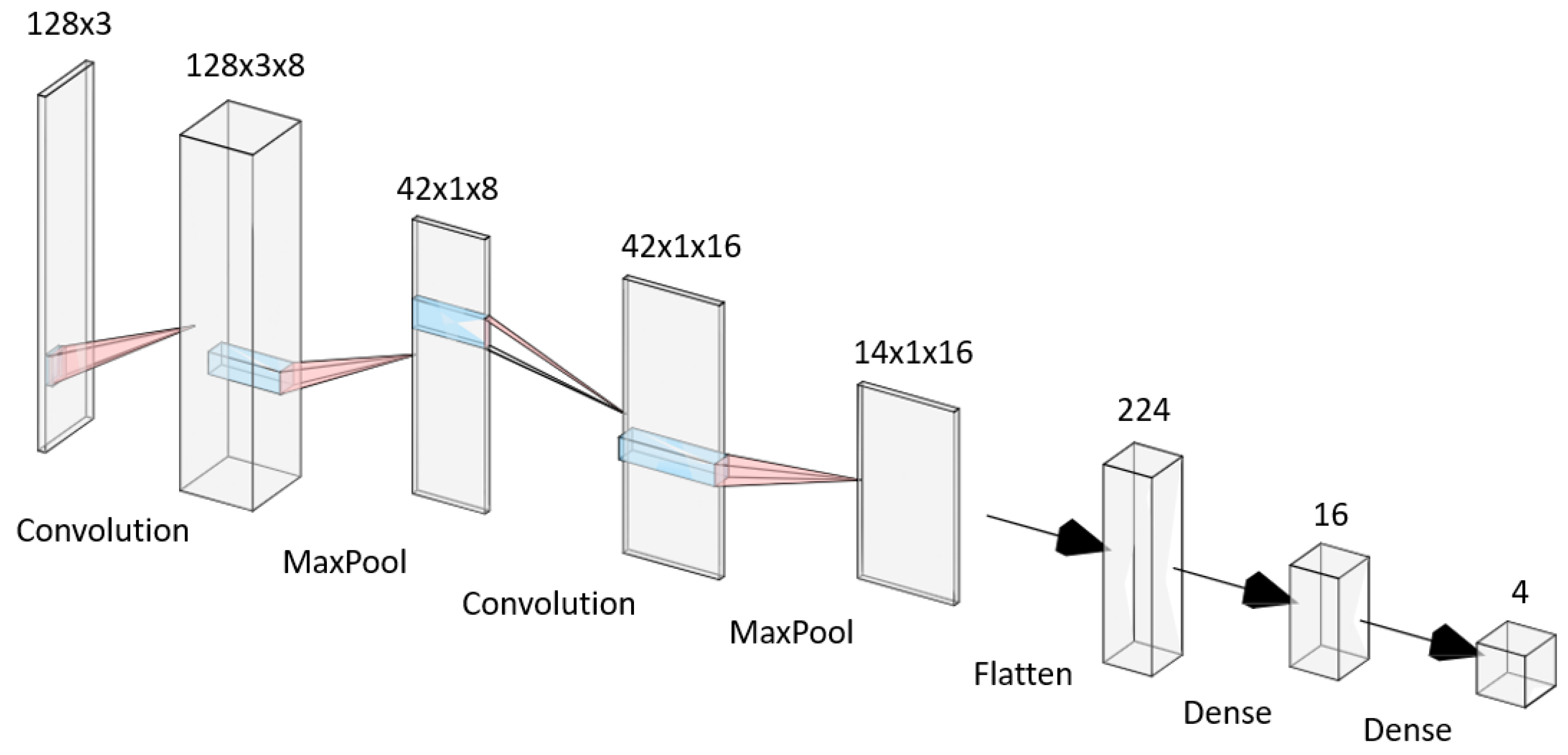
Figure 3.
CLion Code Flowchart.
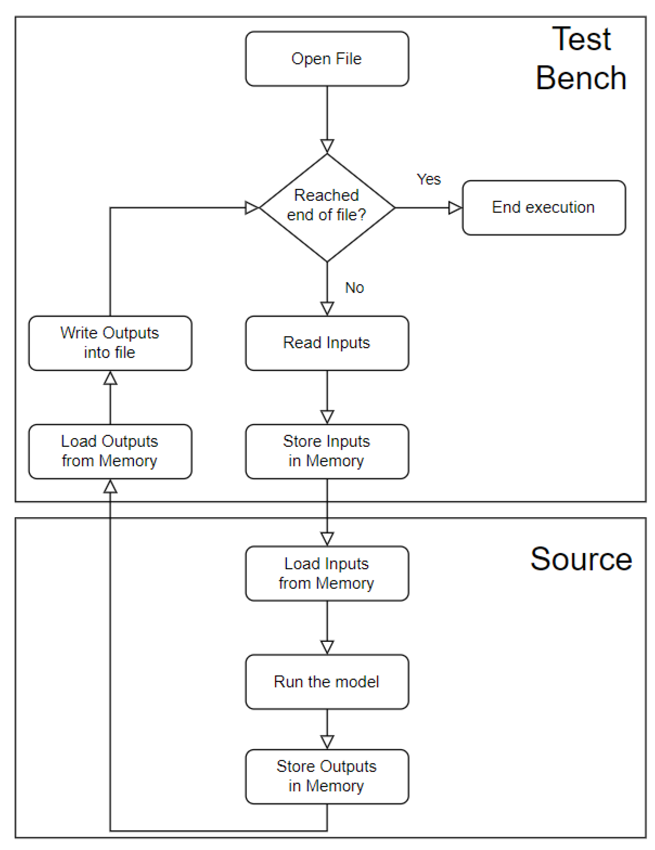
Figure 4.
Dataflow of the model in Vitis HLS.
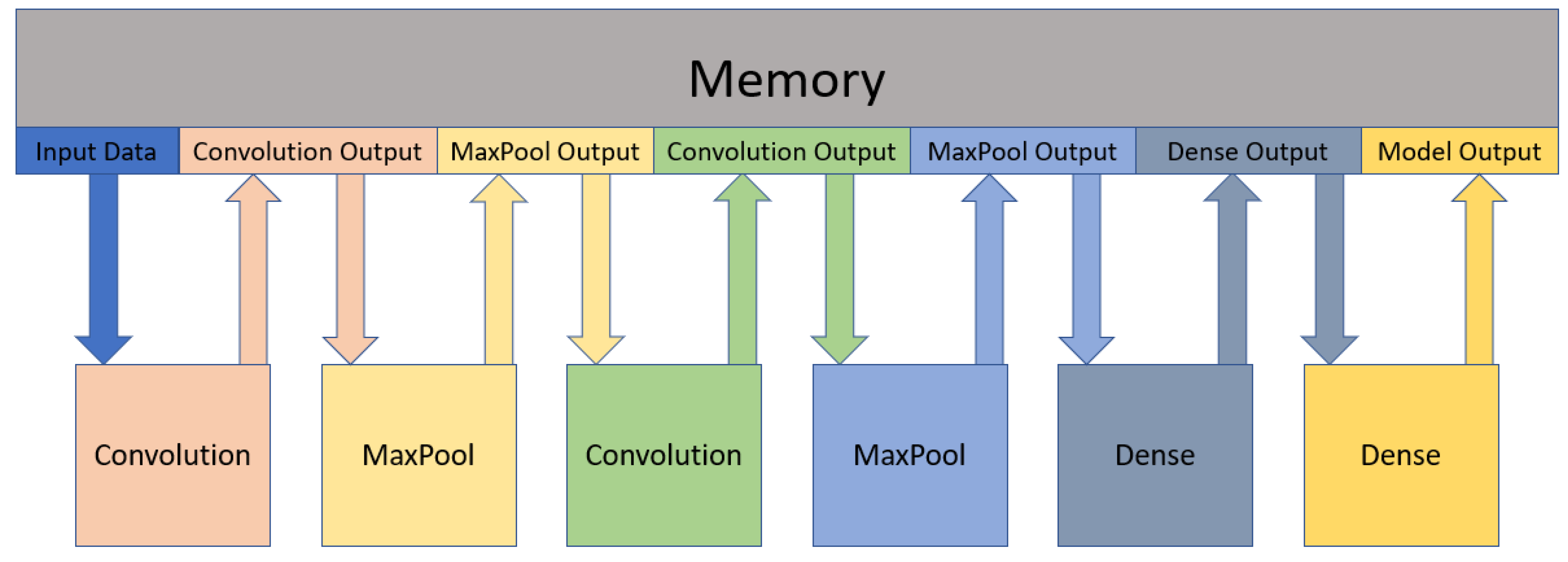
Figure 5.
Graph of the tradeoff between the Resources used (FFs) and Errors of the output values (Maximum Absolute Value) when the wordlength decreases. The left axis corresponds to the Errors. The right axis corresponds to the number of FF’s.
Figure 5.
Graph of the tradeoff between the Resources used (FFs) and Errors of the output values (Maximum Absolute Value) when the wordlength decreases. The left axis corresponds to the Errors. The right axis corresponds to the number of FF’s.
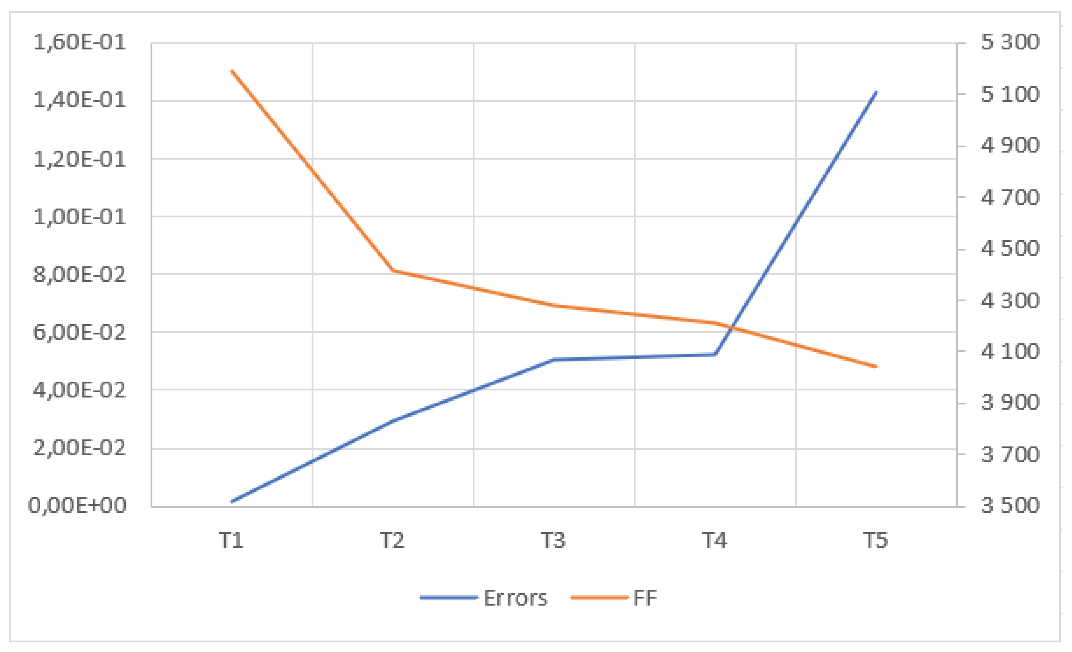

Table 1.
Layers of gesture recognition NN Model.
| Layer | Input Shape | Output Shape | Number of Parameters |
|---|---|---|---|
| Convolution 2D | (128, 3, 1) | (128, 3, 8) | 104 |
| MaxPooling 2D | (128, 3, 8) | (42, 1, 8) | 0 |
| Convolution 2D | (42, 1, 8) | (42, 1, 16) | 528 |
| MaxPooling 2D | (42, 1, 16) | (14, 1, 16) | 0 |
| Flatten | (14, 1, 16) | (224) | 0 |
| Dense | (224) | (16) | 3600 |
| Dense | (16) | (4) | 68 |
Table 2.
Classification errors between the Original TinyML Code and the Custom C Code.
| Gesture | W | O | L | Negative | Total |
|---|---|---|---|---|---|
| Maximum Absolute Error | 1.82E-06 | 1.88E-06 | 2.83E-06 | 2.50E-06 | 2.83E-06 |
| Mean Absolute Error | 1.95E-08 | 6.09E-08 | 1.50E-07 | 1.23E-07 | 8.17E-08 |
| Quadratic Absolute Error | 1.29E-14 | 2.65E-14 | 1.42E-13 | 1.26E-13 | 6.71E-14 |
Table 3.
Errors between the Original TinyML Code and the VitisHLS Code using Floating-Point representation.
Table 3.
Errors between the Original TinyML Code and the VitisHLS Code using Floating-Point representation.
| Gesture | W | O | L | Negative | Total |
|---|---|---|---|---|---|
| Maximum Error | 1.82E-06 | 1.94E-06 | 2.22E-06 | 1.55E-06 | 2.22E-06 |
| Minimum Error | -1.79E-06 | -1.97E-06 | -2.21E-06 | -1.46E-06 | -2.21E-06 |
| Average Error | 2.70E-10 | -1.37E-09 | -8.34E-11 | 1.28E-09 | -2.42E-10 |
| Quadratic Error | 7.08E-15 | 2.47E-14 | 6.35E-14 | 3.54E-14 | 3.21E-14 |
| Standard Deviation | 1.13E-07 | 2.13E-07 | 3.34E-07 | 2.83E-07 | 2.43E-07 |
Table 4.
Errors between the Fixed-Point and the Floating-Point for different rounding modes.
| TRN | TRN_ZERO | RND_ZERO | RND_CONV | |
|---|---|---|---|---|
| Maximum Error | 1.89E-06 | 1.89E-06 | 9.31E-07 | 9.31E-07 |
| Minimum Error | 0.00E+00 | -1.82E-06 | -9.37E-07 | -9.37E-07 |
| Mean Error | 9.43E-07 | -1.50E-07 | 2.90E-08 | 2.90E-08 |
| Mean Absolute Error | 9.43E-07 | 9.78E-07 | 4.47E-07 | 4.47E-07 |
| Quadratic Error | 1.23E-12 | 1.30E-12 | 2.85E-13 | 2.85E-13 |
| Standard Deviation | 5.84E-07 | 1.13E-06 | 5.33E-07 | 5.33E-07 |
| Mode | 1.70E-06 | 8.94E-07 | 7.00E-07 | 7.00E-07 |
| Median | 8.94E-07 | -1.90E-07 | 9.69E-08 | 9.69E-08 |
Table 5.
FPGA resources used for the different Quantization Modes.
| DSP | FF | LUT | |
|---|---|---|---|
| TRN | 2 | 181 | 266 |
| TRN_ZERO | 2 | 182 | 320 |
| RND_ZERO | 2 | 182 | 321 |
| RND_CONV | 2 | 182 | 321 |
Table 6.
Errors between Fixed-Point and Floating-Point after each layer.
| 1st Convolution | 1st MaxPool | 2nd Convolution | 2nd MaxPool | 1st Dense | 2nd Dense | Softmax | |
|---|---|---|---|---|---|---|---|
| Maximum Error | 3.59E-03 | 3.59E-03 | 1.94E-03 | 1.94E-03 | 3.63E-03 | 4.12E-04 | 2.22E-04 |
| Minimum Error | -2.76E-03 | -2.31E-03 | -2.78E-03 | -2.77E-03 | -3.44E-03 | -4.81E-04 | -2.22E-04 |
| Mean Error | -1.00E-06 | 6.39E-05 | -1.18E-05 | -1.22E-05 | -1.12E-04 | 5.25E-06 | 1.05E-08 |
| Mean Absolute Error | 1.51E-04 | 3.76E-04 | 1.22E-04 | 2.22E-04 | 8.87E-04 | 3.14E-04 | 1.11E-04 |
| Quadratic Error | 1.99E-07 | 5.58E-07 | 1.79E-07 | 3.27E-07 | 2.62E-06 | 1.18E-07 | 2.47E-08 |
| Standard Deviation | 4.46E-04 | 7.45E-04 | 4.23E-04 | 5.72E-04 | 1.62E-03 | 3.43E-04 | 1.57E-04 |
| Mode | 0.00 | 0.00 | 0.00 | 0.00 | 0.00 | - | - |
| Median | 0.00 | 0.00 | 0.00 | 0.00 | 0.00 | 0.00 | 0.00 |
Table 7.
Wordlength of each group for the different tests (T1-T5).
| Params | Input | 1st Conv. | 1st MaxPool | 2nd Conv. | 2nd MaxPool | 1st Dense | 2nd Dense | |
|---|---|---|---|---|---|---|---|---|
| T1 | 3.15 | 17.19 | 17.19 | 17.19 | 17.19 | 17.19 | 17.19 | 17.19 |
| T2 | 3.15 | 12.0 | 13.1 | 13.1 | 317.19 | 17.19 | 17.19 | 17.19 |
| T3 | 3.15 | 12.0 | 13.1 | 13.1 | 14.2 | 14.2 | 17.19 | 17.19 |
| T4 | 3.15 | 12.0 | 13.1 | 13.1 | 14.2 | 14.2 | 14.5 | 17.19 |
| T5 | 3.15 | 12.0 | 13.1 | 13.1 | 14.2 | 14.2 | 14.5 | 10.2 |
Table 8.
Errors between the original output values and the output values for the different tests (T1-T5).
Table 8.
Errors between the original output values and the output values for the different tests (T1-T5).
| T1 | T2 | T3 | T4 | T5 | |
|---|---|---|---|---|---|
| Maximum Error | 1.43E-03 | 2.67E-02 | 4.53E-02 | 5.13E-02 | 1.42E-01 |
| Minimum Error | -1.43E-03 | -2.96E-02 | -5.06E-02 | -5.22E-02 | -1.43E-01 |
| Mean Error | -1.53E-10 | 4.53E-11 | -2.28E-10 | -3.44E-10 | -1.07E-10 |
| Mean Absolute Error | 3.76E-05 | 5.70E-04 | 7.64E-04 | 7.63E-04 | 4.49E-03 |
| Quadratic Error | 1.40E-08 | 4.38E-06 | 8.80E-06 | 9.20E-06 | 1.60E-04 |
| Standard Deviation | 1.18E-04 | 2.090E-03 | 2.97E-03 | 3.03E-03 | 1.27E-02 |
| Mode | 0.00 | 0.00 | 0.00 | 0.00 | 0.00 |
| Median | 0.00 | 0.00 | 0.00 | 0.00 | 0.00 |
| Mismatch Predictions | 0 | 0 | 1 | 0 | 7 |
Table 9.
Resources used for the different tests (T0-T5).
| T0 | T1 | T2 | T3 | T4 | T5 | |
|---|---|---|---|---|---|---|
| BRAM | 22 | 19 | 16 | 15 | 15 | 15 |
| DSP | 77 | 77 | 55 | 54 | 53 | 53 |
| FF | 5 647 | 5 190 | 4 418 | 4 277 | 4 212 | 4 044 |
| LUT | 11 336 | 11 175 | 10 952 | 9 816 | 9 859 | 9 685 |
Table 10.
Mismatch Predictions for each Fixed-Point variable group (Convolution and MaxPool Merged for this test). The number inside the parenthesis is the number of bits for the integer part.
Table 10.
Mismatch Predictions for each Fixed-Point variable group (Convolution and MaxPool Merged for this test). The number inside the parenthesis is the number of bits for the integer part.
| Wordlength | Parameters (3) | 1st Conv + MaxPool (13) | 2nd Conv + MaxPool (14) | 1st Dense (14) | 2nd Dense (10) |
|---|---|---|---|---|---|
| 20 | 0 | 0 | 0 | 0 | 0 |
| 19 | 0 | 0 | 2 | 1 | 0 |
| 18 | 0 | 0 | 0 | 0 | 0 |
| 17 | 0 | 0 | 2 | 1 | 1 |
| 16 | 0 | 0 | 1 | 0 | 1 |
| 15 | 0 | 0 | 1 | 3 | 1 |
| 14 | 0 | 0 | 5 | 6 | 2 |
| 13 | 2 | 2 | - | - | 3 |
| 12 | 1 | - | - | - | 5 |
| 11 | 10 | - | - | - | 9 |
| 10 | 8 | - | - | - | 29 |
Table 11.
Wordlength of each group for the different tests (T5-T7).
| Parameters | Input | 1st Convolution | 1st MaxPool | 2nd Convolution | 2nd MaxPool | 1st Dense | 2nd Dense | |
|---|---|---|---|---|---|---|---|---|
| T5 | 3.15 | 12.0 | 13.1 | 13.1 | 14.2 | 14.2 | 14.5 | 10.2 |
| T6 | 3.9 | 12.0 | 13.0 | 13.0 | 14.0 | 14.0 | 14.1 | 10.4 |
| T7 | 3.7 | 12.0 | 13.0 | 13.0 | 14.0 | 14.0 | 14.1 | 10.4 |
Table 12.
Errors between the original output values and the output values for the different test (T5-T7).
Table 12.
Errors between the original output values and the output values for the different test (T5-T7).
| T5 | T6 | T7 | |
|---|---|---|---|
| Maximum Error | 1.42E-01 | 1.11E-01 | 3.41E-01 |
| Minimum Error | -1.43E-01 | -1.06E-01 | -3.41E-01 |
| Mean Error | -1.07E-10 | -2.15E-10 | -5.41E-10 |
| Mean Absolute Error | 4.49E-03 | 3.91E-03 | 1.14E-02 |
| Quadratic Error | 1.60E-04 | 1.26E-04 | 1.15E-03 |
| Standard Deviation | 1.27E-02 | 1.12E-02 | 3.39E-02 |
| Mode | 0.00 | 0.00 | 0.00 |
| Median | 0.00 | -4.40E-25 | 4.41E-11 |
| Mismatch Predictions | 7 | 3 | 12 |
| Bits stored | 144 408 | 113 352 | 104 752 |
Table 13.
FPGA resources used for the different tests (T5-T7).
| T5 | T6 | T7 | |
|---|---|---|---|
| BRAM | 15 | 13 | 12 |
| DSP | 53 | 53 | 53 |
| FF | 4,044 | 3,843 | 3,785 |
| LUT | 9,685 | 9,466 | 9,386 |
Table 14.
Errors between the original output values and the final architecture output values.
| W | O | L | Negative | Total | |
|---|---|---|---|---|---|
| Maximum Error | 2.19E-01 | 1.55E-01 | 2.70E-01 | 3.24E-01 | 3.24E-01 |
| Minimum Error | -1.28E-01 | -1.68E-01 | -2.70E-01 | -3.24E-01 | -3.24E-01 |
| Mean Error | 2.43E-10 | -1.26E-09 | -1.46E-10 | 9.66E-10 | -2.65E-10 |
| Mean Absolute Error | 3.46E-03 | 6.24E-03 | 2.06E-02 | 2.04E-02 | 1.10E-02 |
| Quadratic Error | 3.20E-04 | 3.28E-04 | 2.14E-03 | 2.51E-03 | 1.07E-03 |
| Standard Deviation | 1.79E-02 | 1.81E-02 | 4.63E-02 | 5.01E-02 | 3.28E-02 |
| Mismatch Predictions | 1 | 0 | 7 | 3 | 11 |
| Mismatch Predictions (%) | 0.45% | 0.00% | 3.08% | 4.84% | 1.51% |
Table 15.
Required FPGA resources for different design solutions of this work.
| DS #1 | DS #2 | DS #3 | DS #4 | DS #5 | |
|---|---|---|---|---|---|
| BRAM | 22 | 55 | 50 | 120 | 45 |
| DSP | 77 | 271 | 717 | 302 | 106 |
| FF | 5,647 | 41,483 | 131,136 | 48,793 | 17,526 |
| LUT | 11,336 | 35,891 | 80,022 | 37,704 | 23,042 |
Table 16.
Resources available on a Zynq-7020 SoC-FPGA device.
| BRAM | DSP | FF | LUT |
|---|---|---|---|
| 140 | 220 | 106 400 | 53 200 |
Table 17.
Benchmark Tests for Speedup Performance
| No Pipeline (10ns) | No Pipeline (10.4ns) | |
|---|---|---|
| Clock (ns) | 10.00 | 10.40 |
| Total Time (ns) | 2.644E+06 | 2.739E+06 |
Table 18.
Speedup performance of the architecture when implementing the pipeline optimization on each function/layer.
Table 18.
Speedup performance of the architecture when implementing the pipeline optimization on each function/layer.
| 1st Convolution | 2nd Convolution | 1st MaxPool | 2nd MaxPool | 1st Dense | 2nd Dense | |
|---|---|---|---|---|---|---|
| Clock (ns) | 10.40 | 10.40 | 10.40 | 10.40 | 10.41 | 10.41 |
| Total Time (ns) | 1.408E+06 | 4.780E+05 | 2.760E+05 | 2.550E+05 | 1.020E+05 | 9.913E+04 |
| Function Time - Before (ns) | 1.363E+06 | 9.370E+05 | 2.130E+05 | 2.829E+04 | 1.920E+05 | 3.414E+03 |
| Function Time - After (ns) | 3.221E+04 | 7.592E+03 | 1.063E+04 | 7.114E+03 | 4.37E+04 | 2.390E+02 |
| Function Speedup | 42.3x | 123.4x | 20.0x | 4.0x | 4.6x | 14.3x |
| Total Speedup (10.4ns) | 1.9x | 5.7x | 9.9x | 10.7x | 26.9x | 27.6x |
| Total Speedup (10ns) | 1.9x | 5.5x | 9.6x | 10.4x | 25.9x | 26.7x |
Table 19.
Speedup performance of the architecture when implementing Loop Unroll optimization on a function/layer.
Table 19.
Speedup performance of the architecture when implementing Loop Unroll optimization on a function/layer.
| After Pipeline | 1st Dense (LU) | 1st Convolution (LU) | |
|---|---|---|---|
| Clock (ns) | 10.41 | 10.41 | 10.37 |
| Total Time (ns) | 9.913E+04 | 6.391E+04 | 6.367E+04 |
| Function Time - Before Pipeline (ns) | - | 1.920E+05 | 1.363E+06 |
| Function Time - Before Optimization (ns) | - | 4.137E+04 | 3.224E+04 |
| Function Time - After (ns) | - | 3.727E+03 | 3.212E+04 |
| Function Total Speedup | - | 51.5x | 42.4x |
| Function Optimization Speedup | - | 11.1x | 1.004x |
| Total Speedup (10.4ns) | 27.6x | 42.9x | 43.0x |
| Total Speedup (10ns) | 26.7x | 41.4x | 41.5x |
Table 20.
Speedup performance of the architecture after Merging (M) optimization on functions/layers.
Table 20.
Speedup performance of the architecture after Merging (M) optimization on functions/layers.
| After Pipeline | 1st Conv+Maxpool (M) | 2nd Conv+Maxpool (M) | 2nd Conv+1st Dense (M) | |
|---|---|---|---|---|
| Clock (ns) | 10.41 | 10.37 | 10.37 | 10.37 |
| Total Time (ns) | 9.913E+04 | 5.318E+04 | 4.606E+04 | 4.266E+04 |
| Function Time - Before Pipeline (ns) | - | 1.577E+06 | 9.655E+05 | 1.157E+06 |
| Function Time - Before Optimization (ns) | - | 4.271E+04 | 1.466E+04 | 1.128E+04 |
| Function Time - After (ns) | - | 3.224E+04 | 7.570E+03 | 7.902E+03 |
| Function Total Speedup | - | 48.9x | 127.5x | 146.4x |
| Function Optimization Speedup | - | 1.3x | 1.9x | 1.4x |
| Total Speedup (10.4ns) | 27.6x | 51.5x | 59.5x | 64.2x |
| Total Speedup (10ns) | 26.7x | 49.7x | 57.4x | 62.0x |
Table 21.
Performance comparison.
| Work | Device Used | CNN Model | Performance | FPGA Resources |
|---|---|---|---|---|
| FPGA-based Implementation of a Dynamic Hand Gesture Recognition System [5] | Xilinx Zynq-7000 | CNN | 85% accuracy, 30 FPS | 60% LUTs, 70 DSPs |
| Low Power Embedded Gesture Recognition Using Radar Sensors [6] | Not FPGA-based | CNN + TCN | 92% accuracy | N/A |
| FPGA-based Implementation of Hand Gesture Recognition Using CNN [7] | Xilinx ZCU102 | CNN (ResNet-like) | 75% accuracy, 15 FPS | 72% LUTs, 88 DSPs |
| Implementation of TinyML Models on Arduino 33 BLE [8] | Not FPGA-based | TinyML (DNN) | 80% accuracy, Low latency | N/A |
| A Real-Time Gesture Recognition System with FPGA Acceleration [9] | Xilinx ZCU104 | Modified ZynqNet | 88% accuracy, 60 FPS | 65% LUTs, 96 DSPs |
| Real-Time Implementation of TinyML Models for Hand Gesture Recognition [10] | Not FPGA-based | CNN | 82% accuracy | N/A |
| Real-Time Vision-Based Static Hand Gesture Recognition on FPGA [11] | Xilinx Virtex-7 | CNN + SOM | 78% accuracy, 40 FPS | 58% LUTs, 62 DSPs |
| Hand Gesture Recognition Using TinyML on OpenMV [12] | Not FPGA-based | TinyML (CNN) | 80% accuracy | N/A |
Disclaimer/Publisher’s Note: The statements, opinions and data contained in all publications are solely those of the individual author(s) and contributor(s) and not of MDPI and/or the editor(s). MDPI and/or the editor(s) disclaim responsibility for any injury to people or property resulting from any ideas, methods, instructions or products referred to in the content. |
© 2025 by the authors. Licensee MDPI, Basel, Switzerland. This article is an open access article distributed under the terms and conditions of the Creative Commons Attribution (CC BY) license (http://creativecommons.org/licenses/by/4.0/).
Copyright: This open access article is published under a Creative Commons CC BY 4.0 license, which permit the free download, distribution, and reuse, provided that the author and preprint are cited in any reuse.


