
Submitted:
26 May 2025
Posted:
27 May 2025
You are already at the latest version
Abstract
Large scale traffic simulations at a microscopic level can mimic the physical reality to a great detail and innovative transport services can be evaluated. However, the simulation time of such scenarios is currently too long to be practical. (1) Background: with the availability of Graphical Processing Units (GPUs), is it possible to exploit parallel computing to reduce the simulation time of large microscopic simulations such that they can run on normal PCs at reasonable run-times?; (2) Methods: ParSim, a microsimulator with a monolithic microsimulation kernel has been developed for CUDA compatible GPUs, with the aim to efficiently parallelize the simulation processes, particular care has been taken of the memory usage and thread synchronization, and visualization software has been added optionally; (3) Results: the parallelized simulations have been performed by a GPU with an average performance, the 24h microsimulation scenario of Bologna with 1 million trips has been completed in 40s. Average speeds and waiting times are similar to the results from an established microsimulator (SUMO), but up to 5,000 times faster; the 28 million trips of the 24h San Francisco Bay Area scenario has been completed in 26min. With cutting edge GPUs the simulation speed can possibly be reduced by a factor of 7. (4) Conclusions: the parallelized simulator presented in this paper can perform large scale microsimulation in a reasonable time on available and inexpensive computer hardware. This means microsimulations could now be used in new application fields such as activity-based demand generation, reinforced AI learning, traffic forecasting or crises response management.
Keywords:
microsimulation
; parallelization
; GPU
; traffic assignment
; user-equilibrium
1. Introduction
Simulating individual door-to-door trips of an entire active population is feasible even for large urban areas with today’s computers. A virtual copy of the real population, called synthetic population, is becoming a reality thanks to the availability of big data, large random access memories and faster microprocessors. Modeling the interactions between neighboring vehicles or between vehicles and pedestrians results in precise trip times and speed profiles which allows accurate performance evaluations and transport impact analysis. This is a major advantage enabling accurate assessments such as: 1) the sustainability analysis of various transport policies can be evaluated in what-if scenarios, e.g. additional transport services, new vehicles types or road network modification can be realistically integrated in the model; 2) emergency and evacuation scenarios where determined parts of the transport network are blocked or fail can be tested; 3) the performance and impact of new vehicle technologies can be tested at large scale;.
There are principally two downsides of microsimulations: 1). the modeling can be resource intensive, as many details need to be modeled in the right way, otherwise even smaller modeling errors can lead to catastrophic consequences, and a complete distortion of the results; 2). The long execution time with respect to classical flow-based traffic assignment methods: this is the main reason why microsimulations are not used in Activity Generation, traffic forecasting, AI training and many other time critical applications. This paper addresses the speed issue of current microsimulators and shows that with the use of Graphical Processing Units (GPUs) and by an adequate parallelization and this drawback can be almost entirely overcome.
1.1. State of the Art
Conventional flow-based traffic assignment methods have been invented to determine traffic flows in larger urban road networks, see [1] for a comprehensive overview. These assignment problems could be solved with the limited computing power available during the 60th and 70th. The representation of individual vehicles or even pedestrians of larger-scale scenarios (e.g. with hundreds of thousands of vehicles and people) became only feasible with increasing computing power and memory size at the turn of the century. Different open source projects such as TRANSIMS [2] and SUMO (Simulation of Urban MObility) [3,4] or commercial software such as VISSIM [5], AIMUSUN [6] or DRACULA [7] have been developed. Microsimulation models are typically very detailed, including lanes (with individual access-rights, speed-limits and width), different intersection types (priority, stop, etc.), traffic light systems (TLS) with different Traffic Light Logic (TLL) and different TLS control strategies. The vehicles are essentially represented by the vehicle-following model, which includes driver behavior and a lane change model [3]. The computation time for large-scale microsimulation scenarios is typically slower than in real time [8]. In many applications, traffic assignments run in a loop, for example, during an activity plan generation or user-equilibrium assignment. If thousands of simulation runs are required, then the simulation of a single run should complete in a fraction of the real time.
One possibility of simulating individual vehicles at higher speeds is the use of mesoscopic simulators, which use dynamic queues as a basic edge model. In contrast with microscopic simulations, mesoscopic simulations do not reproduce speed profiles because vehicles in the queue are not coupled with vehicle following models. The mesoscopic simulation platform MATSIM [9] or JDEQSIM are used to generate or calibrate agent based and activity based demand models. JDEQSIM is the simulation engine of the behavior, Energy, and Autonomy Modeling (BEAM CORE) platform [10], where agents can also change plans and routes during the simulation. JDEQSIM has parallelized some algorithms, for example the queing-events or routing can processed in parallel by different cores on the CPU [10]. Also SUMO and other microsimulators have the ability of multi-threating for dedicated tasks, for example the routing [11].
However, none of the established microsimulators exploits the possibility to distribute the computational burden across thousands of GPU cores. One reason may be that it takes considerable efforts to migrate from serialized algorithms implemented for CPUs to parallel algorithms suitable for GPUs.
There have been several attempts to create microsimulators for GPUs from scratch, instead of migrating from an existing code base: the simulator called “Microsimulation Analysis for Network Traffic Assignment” (MANTA) [12,13] and later LPSim [14] is executing microscopic vehicle simulations in parallel on a GPU, including following algorithms, lane change model and a simplified traffic light system. The basic concept of MANTA is a cellular automata, where the lanes of the road network are subdivided into cells of 1 meter length. One lane-cell corresponds to one byte on the GPU memory and if a cell is occupied by a vehicle then its value corresponds to the speed of the respective vehicle, otherwise it defaults to the value of 255. This method is used to identify gaps the vehicles can occupy during lane change maneuvers [14]. The same paper shows that the execution speed of MANTA is orders of magnitudes faster than SUMO for comparable simulation tasks. This speed improvement is significant as it has been demonstrated, for the first time,that a microscopic simulation can be as fast as a mesoscopic simulation. This means that microsimulations could already substitute the previously mentioned mesoscopic simulations in calibration, relaxation and optimization loops used to generate activity based demand models as used in many studies of large scale areas [15,16]. It is worth mentioning that MANTA includes also an optimized routing algorithm which updates link travel times during routing. This algorithm, which runs in parallel on the multiple CPU cores is able to route 3.2 million OD pairs in 62 minutes. Clearly, the routing time has not been included in the simulation time as routing is considered a separate task.
1.2. Objectives
Despite the impressive performance improvements demonstrated by microsimulators running on GPUs, there is ample room for improvements: 1.) the parallelization and respective algorithms can be designed to reduce execution time. GPUs are structured in arrays of blocks, and the data exchange within a block is an order of magnitude faster than the data exchange with the global memory of the GPU. This means there is a trade of between keeping as many as possible information local and to run the simulation on as many as possible blocks in parallel. 2.) the memory usage can be reduced such that even large scale applications with several million trips can run on a single GPU. In case of MANTA, the San Francisco simulation used up to 8 GPUs for a simulation of 24 million trips, which requires a complex and time intensive exchange of information between the GPUs during the simulation runs. To our knowledge, no validation of MANTA has been published.
The objective of this paper is 1) to propose a simulator called ParSim which uses a different parallelization approach with respect to MANTA and 2) to demonstrates its effectiveness in terms of speed, accuracy and usage. The paper is structured as follows: Section 2 describes the basic architecture of the software and explains the most relevant processes; Section 3 shows the simulation results, execution times and validates the GPU based simulation against two SUMO microsimulation models: the City of Bologna, Italy, and the San Francisco Bay Area, California; Section 4 discusses the results, draws relevant conclusions, outlines potential impacts on transport planning and traffic monitoring and suggests further improvements to the presented model.
2. Architecture and Processes
The proposed ParSim simulator is a time-discrete and space-continuous simulator, where the position and speed of active vehicles are updated on the GPU during each step, which corrisponds to a fixed simulated time of seconds. Section 2.1 outlines the vectorized architecture of the data representing the network, while Section 2.2 highlights the representation of vehicles. Additionally, Section 2.3 describes the GPU-based architecture of the parallelized microsimulator.
2.1. Network and Traffic Lights
The network model is composed of arrays, characterizing the network edges, as depicted in Figure 1(a). The network arrays stored in the global GPU memory are summarized on Table 2.
The edge is represented by vectors containing information about length, number of lanes, and maximum allowed speed. Each edge is divided into smaller geometrical segments, which are described by the vectors representing offsets, lengths and angles respectively. These information are used to determine the coordinates of all vehicle on network. Each edge contains one or multiple indexed lanes which are parallel to the edge geometry. Vehicle run on either of them from the start to the end of the edge, the current simulator does not contain a lane-change model to allow for overtaking for example.
Traffic light systems, of any complexity and extension, can be modeled: the principle is that during a red phase, a Traffic Light Logic (TLL) can block the exit of dedicated edges. TTLs are again defined by vectors, representing phase durations and the index of blocked edges during each phase. However, lane-specific traffic lights, for example for dedicated left or right turns, are currently not implemented.
This network architecture is sufficiently memory efficient to allow even larger urban areas to fit in the memory of a single GPU, which are widely available today.
2.2. Vehicle Model
Vehicles are represented by arrays such as position and speed, which are stored in the global GPU memory, see Table 2 for a detailed list.These vehicle states are updated during each simulation step, based on the lead vehicle behavior, constraints by red-light and its position on the current edge and segment. Each vehicle follows a route, which is a sequence of network edges.
The vehicle control follows these basic principles: 1) the vehicle’s acceleration is governed by the Intelligent Driver Model (IDM) [17], which allows the driver to achieve a desired speed, as well as to maintain a safe target headway to the lead vehicle ahead. The used control parameters are shown in Table 1. 2) If the vehicle does not "see" a lead vehicle ahead then the desired speed of the vehicle is set to the minimum of the allowed edge speed and the maximum vehicle speed. 3) In case a leader is assigned, the vehicle tries to converge to a desired time headway to the leader and the desired speed is the speed of the leader. 4) In case the leader changed speed abruptly such that the following vehicle would "crash" into the leader when applying the acceleration from the IDM model, then the follower would instantly adapt to the speed of the leader, regardless the acceleration this maneuver may cause; this means the follower cannot crash into or overtake its leader. This is an important property as it prevents data inconsistencies.
When a vehicle surpasses the end of a segment, it gets place on the next road segment. When a vehicle has arrived at the end of the edge, there are three cases to consider: 1) the vehicle looks into the next edge on its route and checks if there is a sufficiently large gap to allow a safe transition to the next edge; in case the next edge has multiple lanes then the lane with the larges initial gap is chosen; if a sufficiently large gap has been found, then the vehicle transitions to the next edge and looks at the last vehicle on the chosen lane of the next edge. 2) if no sufficiently large gap can be found on either lane of the next edge then the vehicle does not transition, but stops instantly; 3.) if the current edge is controlled by a TLL and the edge is in a red phase then the vehicle will see a "ghost leader" at zero speed, positioned at the end of the edge and will break and stop behind it.
A synchronization algorithm has been put in place, attempting to sequentialize those vehicles running on edges which converge toward the same junction: if a vehicle, positioned on any of the incoming edges, reaches a predefined distance from the downstream junction, then it is appended to a common FIFO queue and the previously last vehicle in the queue becomes the new leader of the newly entered vehicle. This means the order in the queue ultimately defines the sequence in which the vehicles cross the junction. The implemented synchronization technique does ultimately avoid deadlocks at intersection which do occur with other microsimulators [18] , leading to artificial congestion. However, if the incoming edges of a junction are not sufficiently long, then abrupt and unrealistic deceleration do occur as there is not enough room for the necessary speed adaptations.
2.3. Parallel Execution Model
GPUs are able to execute a vast number of threads in parallel. The software library PyCUDA is utilized to implement the simulator. PyCUDA is a Python interface to the CUDA API that facilitates low-level and direct memory management of the GPU as well as the programming and execution of the GPU code, called kernel [19]. With the abstract CUDA concept, threads are grouped in CUDA blocks. The threads in each block are executed by Streaming Multiprocessors (SMs) which consist of multiple CUDA cores. The SM follows the Single Instruction Multiple Data (SIMD) principle [20]. The CUDA Core is the elementary processor that operates on a single data element and recent GPUs integrate a large number (typically thousands) of them. Each thread can simulate, for example, a single vehicle or a single TLL.
The GPU knows two main types of memories: a shared memory which is fast and can only be accessed by a single SM, and the global memory which is slower, but can be seen and accessed by all SMs.
Important software design aspects are: how to distribute the data and how to organize and synchronize the processes such that simulation time is minimized, while respecting limitations in terms of memory size, memory bandwidth and the number of available SMs. These aspects are detailed further below.
The simulator written in PyCUDA has been integrated into the Python-based traffic simulation platform HybridPy [8], which can already interface with SUMO and MATSIM. This means that existing traffic scenarios can be used for testing and evaluation.
2.3.1. Memory Usage
Prior to running the simulation, all arrays regarding infrastructure and vehicles (as defined in Section 2.1 and Section 2.2) are copied into the global memory of the GPU. Our simulation kernel predominantly exploits the global memory, ensuring that a consistent state is maintained among all vehicles and traffic lights. Although slower than shared memory, the global memory is essential for large-scale simulation due to its size and device-wide visibility. The arrays in the global memory, summarized in Table 2, are allocated once and remain during all simulation steps. All threads read and write to the global memory.
The shared memory is used exclusively within the traffic light processing stage. During each simulation step, TLS threads load their timers, active phase indices, program start offsets, and number of phases into shared memory. This enables fast access to control flow data during red-light evaluation and minimizes redundant global memory exchange.
2.3.2. Single-Kernel Fusion Strategy
Once the arrays are placed in the GPU’s memory, the CUDA API launches the kernel on the GPU from the host CPU repeatedly for each simulation step, until the simulation finished. We have adopted a single kernel-fusion strategy, where a single monolithic CUDA kernel updates vehicle position/speed, per-lane vehicle registration, assignment and tracking of lead vehicle as well as traffic light phases. Alternatively, one could consecutively launch multiple kernels, with each performing specific tasks. The multi-kernel approach offers a tidier development environment, as well as having the benefit of modularity and reduced complexity of threads. A single-kernel, although more complex, offers superior performance because of less memory transfers and avoidance of synchronization delays. These observations have been confirmed by Zhang et al. [21], who points out that launching a new kernel is only more preferable in the situation where the performance improvement exceeds the overhead of a new kernel.
2.3.3. Thread Organization and Allocation
The simulation steps are executed with a total number of CUDA threads, which is the sum of active traffic light logics and simulated vehicles , as shown in Figure 2.
The traffic light threads operate concurrently to process their phase timer states, phase transitions and update the state of red-edges, when necessary. The remaining threads, update the vehicle states, as explained in Section 2.2.
This strategy of assigning one thread to each vehicle ensures that the simulation can work and scale well for a large number of vehicles. In addition, it enables a data-parallel execution model and removes inter-thread dependencies. In accordance with NVIDIA’s guidelines, threads are launched in blocks of 256 threads, which helps to balance warp efficiency and occupancy [22]. The number of occupied thread blocks G is obtained by Such a configuration facilitates the dynamic scaling of the thread pool with workload of the simulation while ensuring effective utilization of GPU cores.
2.3.4. Synchronization and Thread Coordination
Synchronization among threads is an important issue as we have adopted a single kernel implementation. In particular, it is vital to carefully consider the synchronization between threads and between the host CPU and the GPU device. Three key methods have been employed for various synchronization tasks:
2.3.4.1. Atomic Operations:
With Atomic operations a thread can perform a memory transaction without interfering with the memory address from any other thread. This ensures a synchronized memory access between parallel threads and prevents race conditions [23]. In our simulation, the following atomic operations are used :
- The atomicOr is used for traffic light threads to mark safely edges as "red" in a bitmask sitting in the global memory. This resolves situations where multiple threads try to signal red-light phases simultaneously.
- The atomicAdd operation tracks the progress of traffic light threads through their update phase.
- The atomicExch is exploited for safe ownership transfer and registration of several parts of the vehicle pipeline. This operation provides the means for proper lane queuing, leader tracking and edge transition even under high concurrency. It ensures the safe assignment of vehicles to a lane, permits the vehicle to become the last one on an edge, and enables the identification of the leader without race conditions.
2.3.4.2. Thread-Level Synchronization
Correctness of shared data, such as red-light state, is a vital part of concurrency in large-scale simulations which was accomplished using a memory fence. In particular, Threadfence() guarantees that all writes to shared and global memory are visible to other threads on the device [24]. Even though, this measure may introduce some delays, the aforementioned necessity to guarantee data integrity makes it unavoidable. In our kernel, this mechanism is used to make sure that traffic light threads update the red-edge mask before vehicle threads access it, thus preventing stale or partial data reads.
2.3.4.3. Host-Device Synchronization
Outside the kernel, appropriate sequencing between simulation steps as well as the prevention of inconsistencies in data or timing during kernel launches are achieved using a host-side synchronization. PyCUDA enables asynchronous kernel invocations by default, meaning they are queued in the GPU, but their completeness is not guaranteed before returning control to the CPU. Host-side barriers are inserted explicitly, to enforce that all processes of one simulation step are completed before the operations on the next step initiate. While multiple kernels can be launched concurrently for performance, we must ensure that all interdependent operations are synchronized [25].
2.4. Visualization
During development, validation, and demonstration of the simulator the visualization is an almost indispensable tool. This is why the simulator can run in GUI-mode (Graphical User Interface mode), where the vehicle movements can be visualized. The HybridPy platform, on which the simulator has been developed, offers already an OpenGl window which allows to view and interact with the network. In gui-mode, vehicle positions and directions are downloaded from the GPU to the CPU after each simulation step and rendered in the OpenGl window together with the network, see screenshot on Figure 3.
In gui-mode, the simulation speed is obviously slowed down considerably by the data downloading operation. The user can add delays such that the human eye can track the motion of individual vehicles, edge and lane transitions and traffic light signals – also single step operations are possible. Note that all simulation speed measurements have been made without the gui-mode.
3. Results
3.1. Test Scenarios
The implemented simulator has been tested with two realistic, large scale scenarios: a smaller scenario of the metropolitan area of Bologna, Italy and a larger scenario with the entire San Francisco Bay Area. The main characteristics of the scenarios are summarized in Table 3.
The Bologna SUMO scenario contains a detailed street network of Bologna city, covering approximately 50 . It includes bikeways and footpath but excludes the rail network. A simplified road network extends into the metropolitan hinterland of Bologna of 3703 ; the entire simulated area has a population of about one million. The road network has been imported from the Openstreetmap [26] and manually refined. The travel demand has been essentially generated from OD matrices: for the core part of the city, the OD matrices has been disaggregated to create a synthetic population with daily travel plans, including the modes car, bicycle, motorcycle and bus. The demand matrices of the hinterland were used to create trips for external and through traffic [27,28]. Public transport services have been created from GTFS data, obtained from the local bus-operator TPER.
For a fair comparison with the parallelized simulation, the following modifications to the original SUMO scenario have been made: 1) within the city area, the SUMO scenario original scenario simulates the door-to-door trip of each person of the synthetic population e.g a person walking from his house to the parking, taking his car, etc; as pedestrians are currently not simulated in ParSim, all walks have been removed and only the vehicle movements have been retained; 2) the original scenario uses the SUMO sub-lane lane-change model, where for example, a car and a bike can stay side by side on the same lane. As such detail is not modeled with the parallelized version, the sub-lane model has been replaced by a simplified model (LANECHANGE2013) where only one vehicle can stay at one place on the lane. 3) the routes have been pre-calculated for the comparison, such that SUMO and ParSim use the exact same routes, no rerouting during the simulation run is performed.
The second scenario is the mesoscopic BEAM CORE model of the entire San Francisco Bay area. The original scenario consist of only 10% of the active population [10]. The BEAM CORE network and the travel plans have been imported into hybridPY. Just as with the Bologna model, only the vehicle trips have been extracted, no pedestrians are simulated. The demand has been upscaled by a factor of 10 by replicating existing routes and randomly varying their departure time by .
Concerning the computer hardware used for the tests, all experiments ran on a laptop with GPU GeForce RTX 4060 from NVIDIA, which contains 3072 Cuda cores and 8 GB of VRAM. The employed CUDA version was 12.8. The host CPU of the laptop has been an Intel i7. Speed measurements are performed in headless mode, allowing ParSim to run at full GPU speed with no rendering overhead. Also the time for uploading of the data arrays in the GPU memory is excluded from the simulation run-time measurements.
3.2. Sensitivity to Number of Trips and Steptime
First we examine with the Bologna scenario how the run-time increases with the number of simulated time steps (e.g. the total simulated time divided by the simulation step time ) and traffic the demand level (e.g. the total number of simulated trips). Figure 4 shows that with a five fold increase of the number of simulation steps (from to ) the run-time increases proportionally by a factor of at demand level.
The higher the demand level, the more dis-proportioned increases the run time: at demand level the run time increases 12 times when simulation steps increase only five times. This effect could be explained by a higher number of vehicle transfers and interactions which means more time spend for atomic exchangers. However, more profiling is needed to identify the cause of the slow down.
Next, the performance gains of ParSim, running on the GPU, versus the original SUMO simulation, running on a single core of the CPU, are investigated. Simulations of the 24h Bologna scenario were repeated under four levels of traffic demand (, , , and ). In each case, the exact same network, trips and routes were used by the simulators, and the simulation run-times were recorded. From the run-times in Table 4 obtained from the Bologna scenario, it is again evident that simulation times increase with an increasing number of traffic. However, the SUMO simulation seems to be more affected than the ParSim simulation. This may be due to difficulties for SUMO to resolve congestion within junction. Such artificial congestion can produce queues that can invade and gridlock the entire network. In fact the average speed of the SUMO simulation dropped below toward the end of the simulation. The teleport (which occurs after 90s standstill) can temporarily resolve mutual blocking by moving vehicles out of the junction onto the next free edge. But this is often not sufficient and the queues continue to grow. In any case, the performance gains of the GPU-based simulations transcend that of SUMO by factors between 1800 and 5000.
The Bologna testbed exhibits a very compact memory footprint: increasing only from 132 at 25 demand to 258 at 50 , 404 at 75 , and just 503 at the full 100 scenario.
The accuracy and reliability of the GPU-based microsimulator has been evaluated by comparing two key indicators obtained from the ParSim and the SUMO simulation: 1) the average Waiting Time which is the sum of all times during which the vehicle’s speed drops below – this is the way SUMO calculates the waiting time (for example in front of traffic lights) 2) the average speed of vehicles during their trips. The results of both the indicators are compared for the two simulators are summarized on Table 5. The waiting times for ParSim are generally lower and the average speeds higher, especially for higher demand levels. The effect can be expected, because of the simpler intersection model of ParSim with respect to SUMO.
The demand level has not been evaluated since the SUMO simulation showed excessive congestion due to artificial deadlocks at intersections. Also the demand level resulted in havy congestions and girdlocks, this is why the SUMO waiting time are considerably higher then those of ParSim for this scenario.
3.3. Performance Comparison with S.F. Bay Area Scenario
The full 24-hour scenario of S.F. the Bay Area with 18 million trips and a rush hour scenario from 7:00 to 9:00 with 3 million trips have been used to compare the ParSim simulator presented in this work with the LPsim parallel microsimlator implementation previously developed in [14]. The ParSim simulator has completed the 24h scenario in 1,534.68 s or 25.58 min on a single GPU with 8GB of memory. The same scenario has been simulated with LPsim using 4xNvidia A100 graphic cards with 40GB each. Comparing ParSim with LPSim, it can be concluded that ParSim finished the rush hour 7 times faster while occupying a much less memory on the GPU. These two quantities are related as the communication between multiple GPU will slow down the overall simulation process.
4. Discussion
4.1. Main Results
The main results are that ParSim, the microsimulator based on parallel computing, is approximately 3000 times faster than a similar SUMO simulation on a single core CPU. The 1 million trips of the 24h Bologna scenario could be finished in just 41s, while it took 26 min for the completion of the larger 24h, 18 million trip Bay area scenario. The simulator is also 7 times faster than a previously proposed parallelized simulator called LPsim and has a much lower memory footprint too. However, it needs to be acknowledged that LPsim has a more details lane change model that allows overtaking.
The simulation results of ParSim have been validated by comparing average waiting times and average speeds with the output of the established microsimulator SUMO. The average travel speeds of the vehicles of Parsim where approximately 10% higher compared with the average speed determined by SUMO, presumably due to the simplier intersection model of ParSim. In addition, ParSim has the possibility of visual verification and debugging through a GUI. The visualization turned out to be crucial for code writing and debugging. It can also be helpful for network planning tasks.
The success of the presented simulator is based on multiple design decisions:
- the network and vehicle model have been implemented such that the occupied memory on the GPU is minimized. We have shown that even large scale simulation, like the one of San Francisco Bay area with 8 million inhabitants can fit on a medium grade GPU with 8GB of ram. The fact that all processes take place on a single GPU is a speed advantage with respect to a solution with multiple GPUs.
- the entire simulator has been implemented on a single monolithic kernel, which saves time lost while swapping kernels between CPU and GPU.
- the implementation of the single kernel introduced some complexity because we had to ensure that threads during a simulation step are synchronized and processed in a certain temporal order. Different synchronization techniques, such as atomic exchangers or memory fences have been used to accomplish this.
4.2. New Applications for Microsimulations
It appears obvious that with the shortened simulation times, microsimulation models can now be employed in a series of applications where they had been too slow in the past. In addition, the ParSim simulator can run on ordinary gaming computers, no expensive hardware is necessary. Potential applications for parallelized microsimulators like ParSim include:
- microsimulations as principle assignment method for the activity/plan generation as part of agent based demand models, where traffic assignment are in a loop and need to be repeated many times. This application may facilitate the creation of larger mobility digital twins of entire cities.
- Training AI agents, such as reinforcement learning or deep RL models, where millions of simulation episodes are needed to converge.
- Traffic optimization studies, where the system evaluates control strategies, route planning, or congestion mitigation across hundreds of randomized or adaptive scenarios.
- short term traffic predictions based on real time flow measurements.
- Crisis response simulation, enabling fast forecasting of network behavior under incidents or disruptions and supporting real-time decision-making.
4.3. Limitations
The current version of the ParSim simulator is lacking of some useful functionality, which would make the microsimulation model more realistic. Some desirable features would be: lane-to-lane connections within junctions, together with lane-based traffic light programs; an improved lane-change model, pedestrians and pedestrian crossings. There is also a lack of flexibility when it comes to producing output of various types from the simulation.
4.4. Future Developments
Some of the above mentioned limitations could be implemented without slowing down the GPU significantly. One useful extension would be to enable re-routing during the simulation. This feature would allow more realistic traffic assignments as well as ride-sharing, and ride hailing transport services.
Our simulation design is not limited to a certain GPU type, and can easily be ported to newer and more advanced chips with a higher number of CUDA cores – this would immediately result in a higher simulation speed. We also expect a notably better performance on GPUs with higher memory bandwidth and improved scheduling efficiency. Larger vehicle population could be simulated in parallel, without the need to fundamentally alter the code design. For instance, an NVIDIA RTX 5090-with 21,760 CUDA cores, one of the high-end GPUs, has 7 times more cores than the GPU used in the present study.
Author Contributions
Conceptualization, J.S. and B.H.; methodology, B.H. and J.S.; software, B.H. and J.S..; validation, B.H., N.N.; formal analysis, B.H.; investigation, B.H.; resources, C.P. and N.N.; data curation, N.N., C.P. and J.S; writing—original draft preparation, J.S. and B.H.; writing—review and editing, B.H. and C.P; visualization, B.H. and J.S.; supervision, J.S.; project administration, J.S. and F.R.; funding acquisition, F.R. All authors have read and agreed to the published version of the manuscript.
Funding
This project is co-founded by the ECO SISTER and the HPC project, both financed by the Italian PNRR programme.
Data Availability Statement
The developed software ParSim is under a licensing process and is currently not publicly available. SUMO, BEAM and MANTA are open-source software and available on Github.
Conflicts of Interest
The authors declare no conflicts of interest.
Abbreviations
The following abbreviations are used in this manuscript:
| GPU | Graphical Processing Unit |
| CUDA | Compute Unified Device Architecture |
| API | Application Programming Interface |
| MPs | Multi Processors |
References
- Patriksson, M. The Traffic Assignment Problem: Models and Methods; 2015.
- Lee, K.S.; Eom, J.K.; seop Moon, D. Applications of TRANSIMS in Transportation: A Literature Review. Procedia Computer Science 2014, 32, 769–773. [Google Scholar] [CrossRef]
- Krajzewicz, D.; Erdmann, J.; Behrisch, M.; Bieker, L. Recent Development and Applications of SUMO - Simulation of Urban MObility. International Journal On Advances in Systems and Measurements 2012, 5, 128–138. [Google Scholar]
- Koch, L. ; , D.S.B.; Wegener, M.; Schoenberg, S.; Badalian, K.; Dressler, F.; Andert, 2021, J. Accurate physics-based modeling of electric vehicle energy consumption in the SUMO traffic microsimulator. In Proceedings of the 2021 IEEE International Intelligent Transportation Systems Conference (ITSC); pp. 1650–1657. [Google Scholar] [CrossRef]
- Fellendorf, M.; Vortisch, P. Microscopic traffic flow simulator VISSIM, 2011. [CrossRef]
- Anya, A.; Rouphail, N.; Frey, H.; Schroeder, B. Application of AIMSUN Microsimulation Model to Estimate Emissions on Signalized Arterial Corridors. Transportation Research Record: Journal of the Transportation Research Board 2014, 2428, 75–86. [Google Scholar] [CrossRef]
- Liu, R. , The DRACULA Dynamic Network Microsimulation Model; 2005; Vol. 31, pp. 23–56. [CrossRef]
- Schweizer, J.; Schuhmann, F.; Poliziani, C. hybridPy: The Simulation Suite for Mesoscopic and Microscopic Traffic Simulations. SUMO Conference Proceedings 2024, 5, 39–55. [Google Scholar] [CrossRef]
- Auld, J.; Hope, M.; Ley, H.; Sokolov, V.; Xu, B.; Zhang, K. POLARIS: Agent-based modeling framework development and implementation for integrated travel demand and network and operations simulations. Transportation Research Part C: Emerging Technologies 2016, 64, 101–116. [Google Scholar] [CrossRef]
- Spurlock, C.A.; Bouzaghrane, M.A.; Brooker, A.; Caicedo, J.; Gonder, J.; Holden, J.; Jeong, K.; Jin, L.; Laarabi, H.; Needell, Z.; et al. Behavior, Energy, Autonomy & Mobility Comprehensive Regional Evaluator: Overview, calibration and validation summary of an agent-based integrated regional transportation modeling workflow. Technical report, Berkeley, 2024. [Google Scholar]
- DLR. SUMO User Documentation: duarouter. https://sumo.dlr.de/docs/duarouter.html, last seen 25. 20 May.
- Yedavalli, P.; Kumar, K.; Waddell, P. 2021; arXiv:physics.soc-ph/2007.03614].
- Waddell, P. SimUAM: A Comprehensive Microsimulation Toolchain to Evaluate the Impact of Urban Air Mobility in Metropolitan Areas. RePEc: Research Papers in Economics.
- Jiang, X.; Sengupta, R.; Demmel, J.; Williams, S. Large scale multi-GPU based parallel traffic simulation for accelerated traffic assignment and propagation. Transportation Research Part C: Emerging Technologies 2024, 169, 104873. [Google Scholar] [CrossRef]
- Balmer, M.; Axhausen, K.; Nagel, K. Agent-Based Demand-Modeling Framework for Large-Scale Microsimulations. Transportation Research Record 2006, 1985, 125–134. [Google Scholar] [CrossRef]
- Maciejewski, M.; Nagel, K. Towards Multi-Agent Simulation of the Dynamic Vehicle Routing Problem in MATSim. In Proceedings of the Parallel Processing and Applied Mathematics; Wyrzykowski, R.; Dongarra, J.; Karczewski, K.; Wasniewski, J., Eds., Berlin, Heidelberg; 2012; pp. 551–560. [Google Scholar]
- Treiber, M.; Hennecke, A.; Helbing, D. Congested traffic states in empirical observations and microscopic simulations. Physical review E 2000, 62, 1805. [Google Scholar] [CrossRef] [PubMed]
- DLR. SUMO User Documentation: Why Vehicles are teleporting. https://sumo.dlr.de/docs/Simulation/Why_Vehicles_are_teleporting.html, last seen 25. 20 May.
- Klöckner, A.; Pinto, N.; Lee, Y.; Catanzaro, B.; Ivanov, P.; Fasih, A. PyCUDA and PyOpenCL: A Scripting-Based Approach to GPU Run-Time Code Generation. Parallel Computing 2012, 38, 157–174. [Google Scholar] [CrossRef]
- Egielski, I.J.; Huang, J.; Zhang, E.Z. Massive atomics for massive parallelism on GPUs. In Proceedings of the Proceedings of the 2014 International Symposium on Memory Management, New York, NY, USA, 2014. [CrossRef]
- Zhang, L.; Wahib, M.; Matsuoka, S. Understanding the overheads of launching CUDA kernels. ICPP19.
- NVIDIA Corporation. CUDA C++ Programming Guide, /: Version 12.9, https; .9.
- Dang, H.V.; Schmidt, B. CUDA-enabled Sparse Matrix–Vector Multiplication on GPUs using atomic operations. Parallel Computing 2013, 39, 737–750. [Google Scholar] [CrossRef]
- Feng, W.c.; Xiao, S. To GPU synchronize or not GPU synchronize? In Proceedings of the 2010 IEEE International Symposium on Circuits and Systems (ISCAS); 2010; pp. 3801–3804. [Google Scholar] [CrossRef]
- Tuomanen, B. Hands-On GPU Programming with Python and CUDA: Explore high-performance parallel computing with CUDA; Packt Publishing Ltd, 2018.
- OpenStreetMap. http://www.openstreetmap.org/.
- Nguyen, N.A.; Poliziani, C.; Schweizer, J.; Rupi, F.; Vivaldo, V. Towards a Daily Agent-Based Transport System Model for Microscopic Simulation, Based on Peak Hour O-D Matrices. In Proceedings of the Computational Science and Its Applications – ICCSA 2024; Gervasi, O.; Beniamino, M.; Garau, C.; Taniar, D.; Rocha, C.; Ana, M.A.; Lago, F.; Noelia, M., Eds., Cham; 2024; pp. 331–345. [Google Scholar]
- Schweizer, J.; Poliziani, C.; Rupi, F.; Morgano, D.; Magi, M. Building a large-scale micro-simulation transport scenario using big data. ISPRS INTERNATIONAL JOURNAL OF GEO-INFORMATION 2021, 10, 165–174. [Google Scholar] [CrossRef]
Figure 1.
Scheme with basic elements and quantities of the parallelized simulation model. (a) Network representation: Each edge is subdivided in one or several segments in the longitudinal direction and lanes in the transversal direction. Note that the follower vehicle 2 is able to look ahead and recognize the distance to vehicle 1. (b) the quantities necessary to calculate the vehicle acceleration using the IDM vehicle following model, as explained in Section 2.2.

Figure 2.
Scheme shows how Traffic Light Logic (TLL) threads and vehicle threads are organized on the GPU.
Figure 2.
Scheme shows how Traffic Light Logic (TLL) threads and vehicle threads are organized on the GPU.
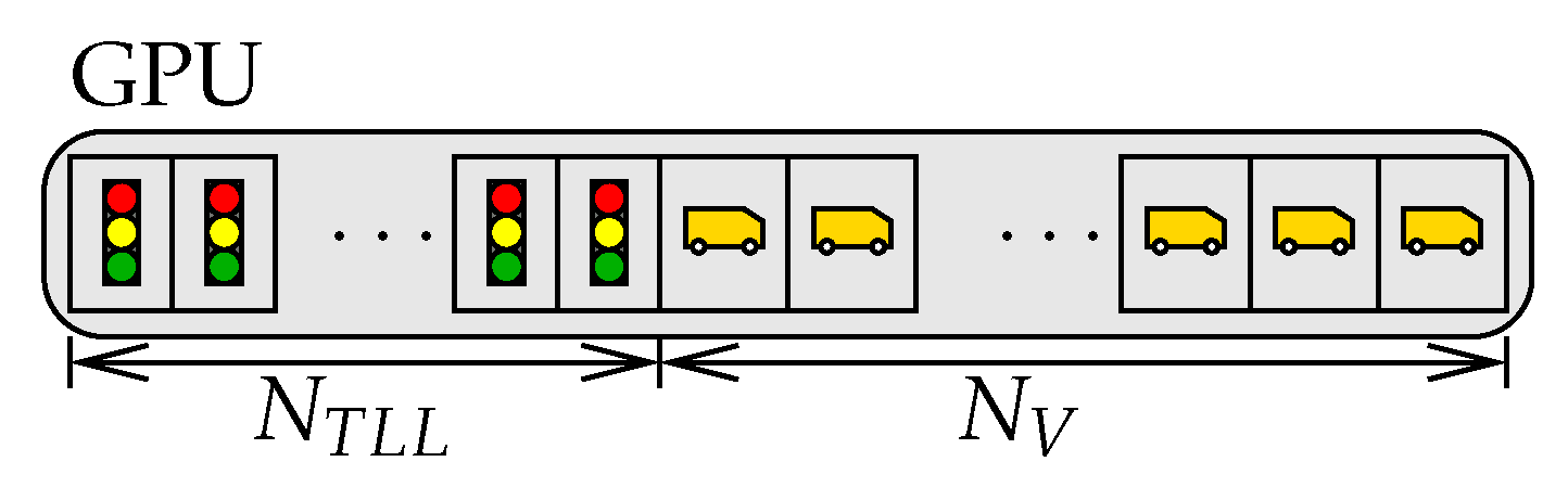
Figure 3.
Graphical User Interface of HybridPy with data browser (left panel) and interactive Network visualization (in blue) with vehicles (in yellow). Below the network are the buttons to operate the ParSim. Note the vehicle queues waiting at a traffic light and two bicycles running on the red bikepath.
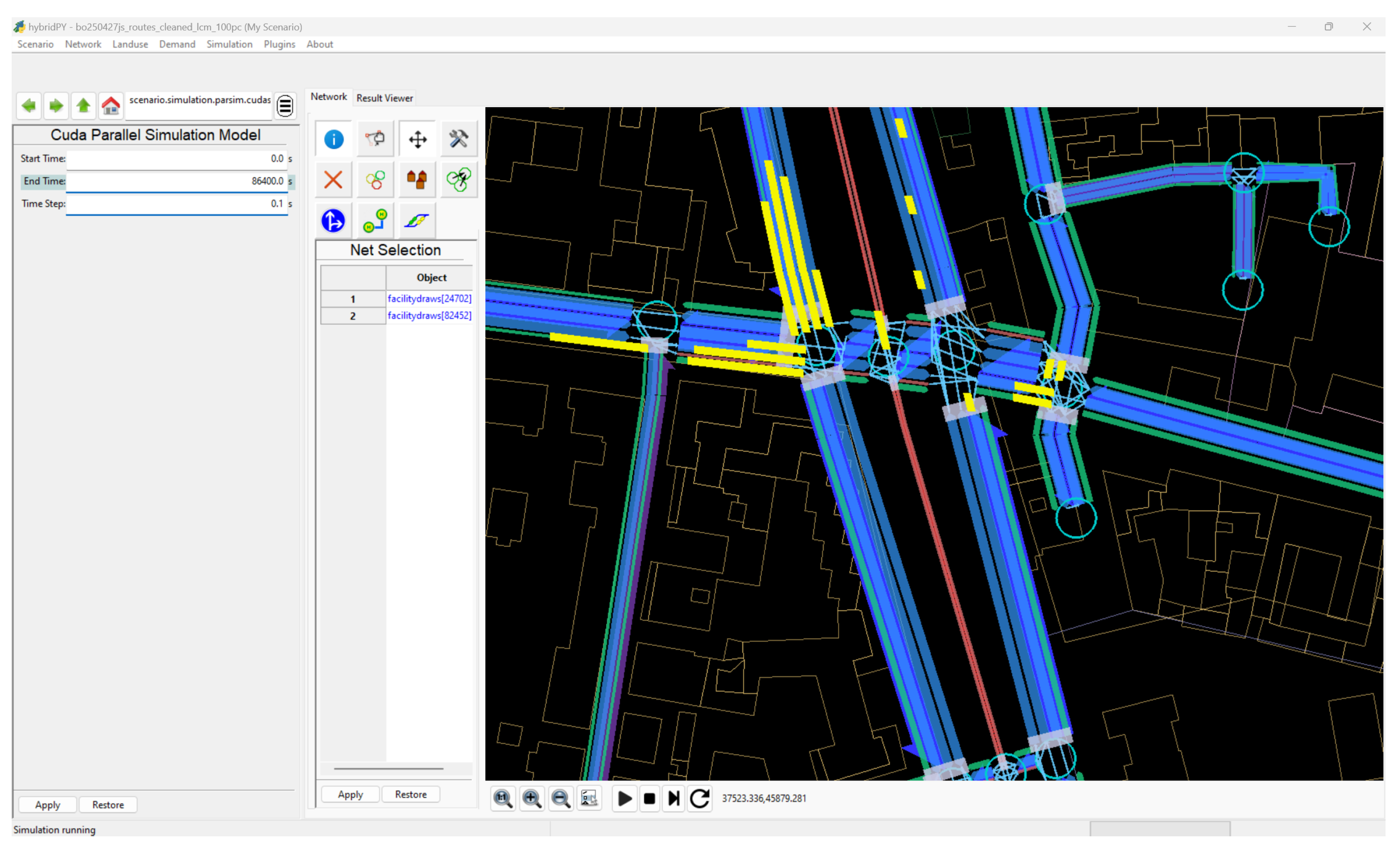
Figure 4.
Increase of simulation run time with an increasing number of iterations and demand level of the Bologna scenario. Note the logarithmic scale of the simulation run time.
Figure 4.
Increase of simulation run time with an increasing number of iterations and demand level of the Bologna scenario. Note the logarithmic scale of the simulation run time.
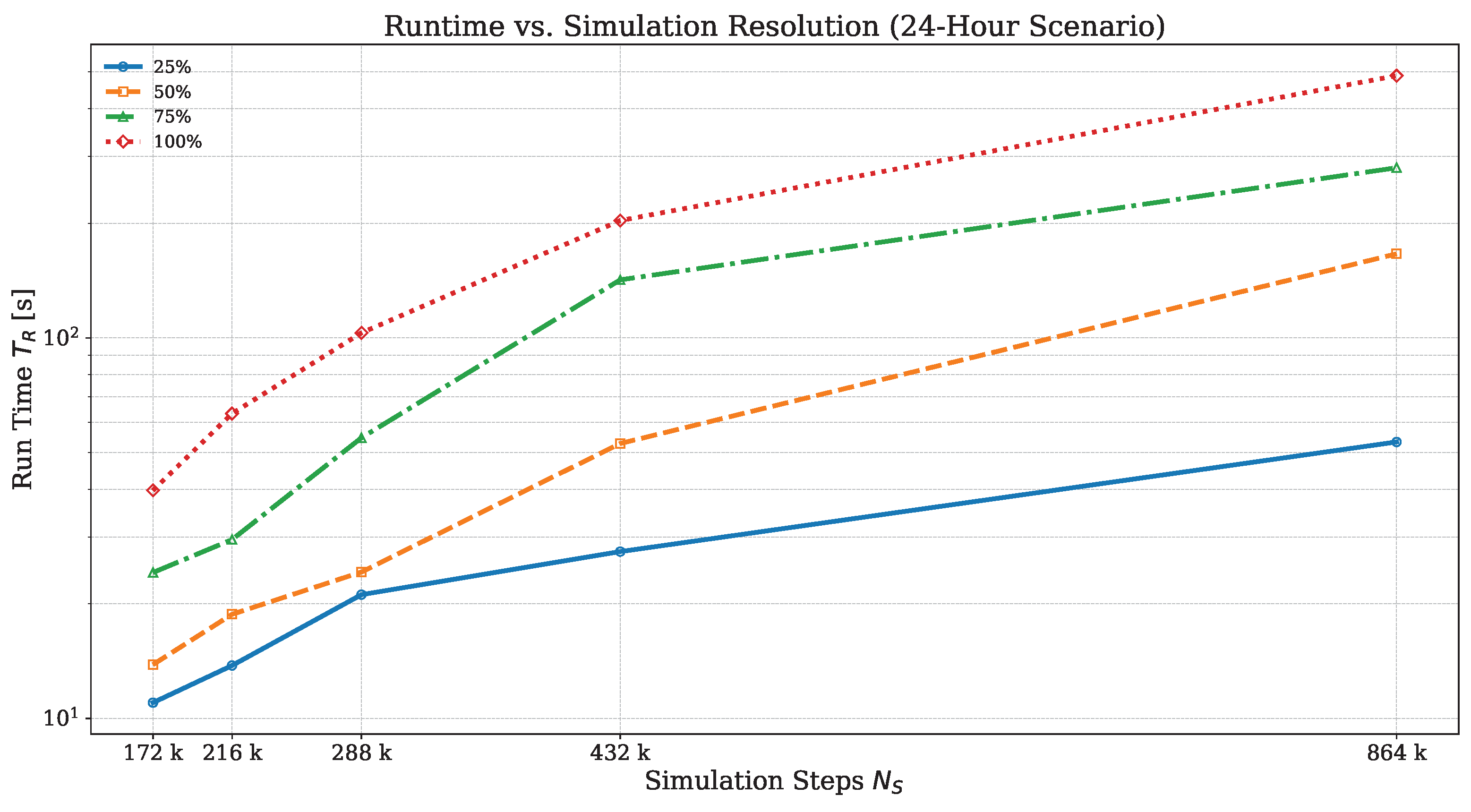

Table 1.
Used variables for the IDM (according to [17]).
Table 1.
Used variables for the IDM (according to [17]).
| Parameters | Variable | Value |
|---|---|---|
| Maximum acceleration | a | 2.5 |
| Desired deceleration | b | 1.8 |
| Target time headway | 1.5 | |
| Minimum spacing | 3.0 | |
| Length of the vehicle | l | 5.0 |
| Acceleration exponent | 4.0 |
Table 2.
Arrays of the gloal memory.
| Domain | Arrays |
|---|---|
| Vehicle states: | position, speed, edge and segment index, lane index, route pointer, route array, odometer, and leader references |
| Network | segment lengths, geometry vectors, offsets, speed limits, and forward edge tree |
| Control structures | route matrices, lane queues, vehicle-linked lists, red-light masks, and occupancy maps. |
| Traffic control data: | timers, phase indices, and program offsets for each traffic light. |
Table 3.
Characteristics of the scenarios.
| Bologna | S.F. Bay Area | |
|---|---|---|
| Total edges | 58,882 | 181,932 |
| Total length [km] | 3,737 | 45,060 |
| Number of trips | 1 M | 18 MiMo |
| Number of TTL | 312 | - |
Table 4.
Simulation run-time comparison between ParSim (on GPU) and SUMO (on CPU) for the Bologna scenario.
Table 4.
Simulation run-time comparison between ParSim (on GPU) and SUMO (on CPU) for the Bologna scenario.
| Traffic Demand | SUMO (CPU) | ParSim (GPU) | Speed gain |
|---|---|---|---|
| 25% | 20,376 s | 11.00 s | 1852 |
| 50% | 49,356 s | 13.85 s | 3563 |
| 75% | 88,128 s | 24.18 s | 3644 |
| 100% | 200,916 s | 39.76 s | 5053 |
Table 5.
Comparison of ParSim and SUMO Simulation Outputs.
| Traffic Demand | Avg. Waiting Time [s] | Avg. Speed [m/s] | ||
|---|---|---|---|---|
| ParSim | SUMO | ParSim | SUMO | |
| 25% | 51.00 | 61.27 | 17.30 | 15.45 |
| 50% | 76.65 | 98.53 | 16.88 | 14.33 |
| 75% | 121.74 | 743.78 | 15.75 | 12.88 |
Table 6.
Performance comparison between ParSim and LPsim.
| Scenario | Run-time [s] | Memory footprint[GB] | ||
|---|---|---|---|---|
| ParSim | LPsim | ParSim | LPsim | |
| 24h, 18 M trips | 1534.68 | - | 5.07 | ≈160 |
| Rush hour, 3 M trips | 21.73 | 144 | 0.826 | ≈40 |
Disclaimer/Publisher’s Note: The statements, opinions and data contained in all publications are solely those of the individual author(s) and contributor(s) and not of MDPI and/or the editor(s). MDPI and/or the editor(s) disclaim responsibility for any injury to people or property resulting from any ideas, methods, instructions or products referred to in the content. |
© 2025 by the authors. Licensee MDPI, Basel, Switzerland. This article is an open access article distributed under the terms and conditions of the Creative Commons Attribution (CC BY) license (https://creativecommons.org/licenses/by/4.0/).
Copyright: This open access article is published under a Creative Commons CC BY 4.0 license, which permit the free download, distribution, and reuse, provided that the author and preprint are cited in any reuse.


