Submitted:
26 May 2025
Posted:
26 May 2025
You are already at the latest version
Abstract
Cascading link failures continue to imperil power grids, transport networks and cyber-physical systems, yet the relationship between a network’s robustness at the moment of attack and its subsequent resiliency remains poorly understood. We introduce a dynamic framework in which connectivity-based cascades and distributed self-healing act concurrently within each time-step. Failure is triggered when a node’s active-neighbor ratio falls below a threshold φ; healing activates once the global fraction of inactive nodes exceeds a trigger T and is limited by a budget B. Two real data sets—a 332-node U.S. airport graph and a 1133-node university e-mail graph—serve as testbeds.
For each graph we sweep the parameter quartet (φ, B, T,attack mode) and record (i) immediate robustness R, (ii) 90 % recovery time T90, and (iii) cumulative average damage. Results show that targeted hub removal is up to three times more damaging than random failure, but that prompt healing with B≥0.12 can halve T90. Scatter-plot analysis reveals a non-monotonic correlation: high-R states recover quickly only when B and T are favorable, whereas low-R states can rebound rapidly under ample budgets. A multiplicative fit T_90 ∝B^(-β) g(T)h(R) (with β≈1) captures these interactions.
The findings demonstrate that structural hardening alone cannot guarantee fast recovery; resource-aware, early-triggered self-healing is the decisive factor. The proposed model and data-driven insights provide a quantitative basis for designing infrastructure that is both robust to failure and resilient in restoration.
Keywords:
cascading failure
; connectivity-based model
; robustness–resiliency correlation
; self-healing networks
; cybersecurity
; recovery time
; average damage
; budget–trigger trade-off
; complex infrastructure networks
1. Introduction
Modern infrastructure, from transportation and power grids to digital communication and finance, is increasingly organized as interacting networks. When a local fault occurs, the disturbance can propagate through the web of inter-node dependencies, potentially disabling a large fraction of the system. Two complementary performance concepts are therefore central to design:
- Robustness is the ability of the system to withstand the initial disturbance; it is often quantified by the fraction of components that remain functional immediately after the shock [1].
- Resiliency (or recovery) is the ability to return to acceptable performance after the disturbance. It combines the depth of degradation with the speed and extent of restoration [2].
Because many critical sectors now demand guarantees on both attributes [3,4], understanding how robustness and resiliency interact has become an urgent research topic.
Many real-world systems have been widely modeled as networked complex systems such as communication networks[5], power grids[6,7], command and control systems[8,9], financial transaction systems [10]. Therefore, a better understanding of both terminologies and the interplay among them is essential in prolonging the performance sustainability of modern society infrastructures.
1.1. Existing Work on Cascading Failures
Cascading-failure models fall into two broad classes. Connectivity-based models—pioneered by Watts [11]—assume a node becomes inactive when the fraction of its active neighbours drops below a threshold. They have been used to study opinion shifts, information diffusion, virus spreading and community effects [12]. Load-based models, exemplified by Motter & Lai [13], track the redistribution of traffic or flow after a node failure and disable any node whose new load exceeds its capacity. Each paradigm has generated a large body of robustness studies, including targeted attacks on interdependent networks [14], the influence of clustering [15], degree-distribution breadth [16] and optimal interlinking strategies [17].
By contrast, few studies incorporate explicit recovery processes. Early work on network “self-healing’’ proposed instantaneous re-wiring or capacity boosts [18,19,20,21], but did not model the temporal competition between failure propagation and repair. Liu et al. [22] introduced a concurrent self-healing rule for overload cascades, yet the literature still lacks a systematic analysis of how recovery parameters modify the robustness–resiliency trade-off. Metrics for post-disaster performance: resilience triangles [23], disruption cost [24], agent-based restoration times [25]—have been proposed, but none link those metrics back to the pre-failure robustness of the same network.
1.2. Objectives and Contributions of This Work
This paper focuses exclusively on the connectivity-based (link-breaking) cascade and augments it with a dynamic self-healing mechanism that operates concurrently with failure propagation. Building on that framework we make four contributions:
- 1.
- Concurrent cascade + self-healing model. We formulate two algorithms: one for link-breaking failure and one for distributed healing, that act within the same simulation step, controlled by a budget parameter and a triggering threshold .
- 2.
- Quantitative evaluation on real data. Using a U.S. airport network (332 nodes) [26] and a university e-mail network (1133 nodes) we measure robustness and two resiliency metrics: 90 % recovery time T90 and cumulative average damage.
- 3.
- Systematic exploration of parameter space. We vary the degree-loss threshold , the attack mode (random vs. targeted), the healing budget and the trigger time, producing a comprehensive map of robustness and resiliency responses.
- 4.
- First empirical correlation study. Scatter-plot analysis reveals that robustness and resiliency are only weakly correlated unless the trigger is early and the budget adequate; high robustness can coexist with slow or costly recovery and vice versa. We summarize the relationship with a simple multiplicative fit and discuss design implications.
1.3. Paper Organization
Section II introduces the connectivity-based model, the self-healing algorithm, and the data sets. Section III presents robustness results, resiliency results, and their correlation. Section IV concludes and outlines directions for recovery-aware network design.
2. Description of Models and Methods
In this section we outline the mechanism used to model the cascading-failure (CF) phenomenon that often arises in networked systems subjected to disruptions.
2.1. Connectivity – Based Failure and Healing
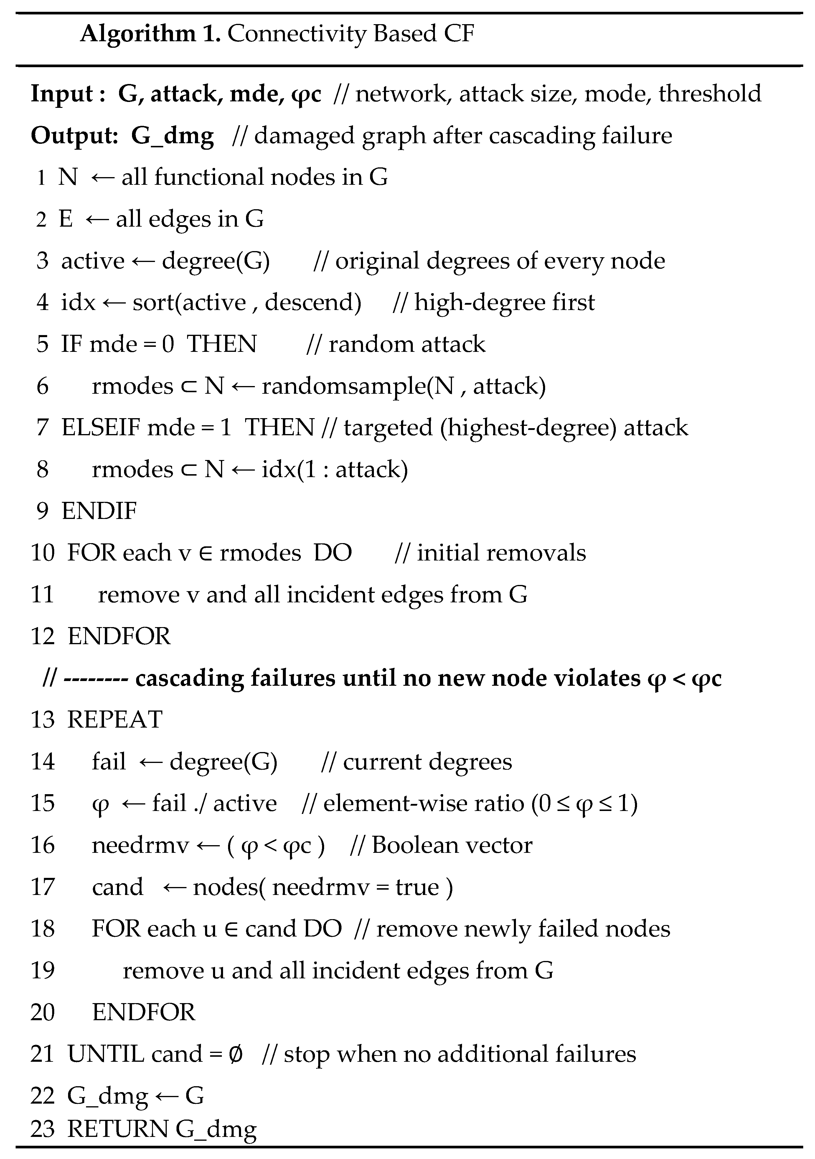
A connectivity-based (link-breaking) cascade proceeds as described in Algorithm 1. In the original graph G a set of nodes is initially attacked. Those attacked nodes, together with all incident links, are removed and become inactive. The initial set can be chosen randomly or by targeting high-degree hubs.After the attack, the algorithm scans each remaining active node and computes the ratio
If falls below a critical threshold , the node is scheduled to fail in the next step. The failure–check cycle repeats until the graph reaches a steady state in which some (or all) of the original nodes are inactive.
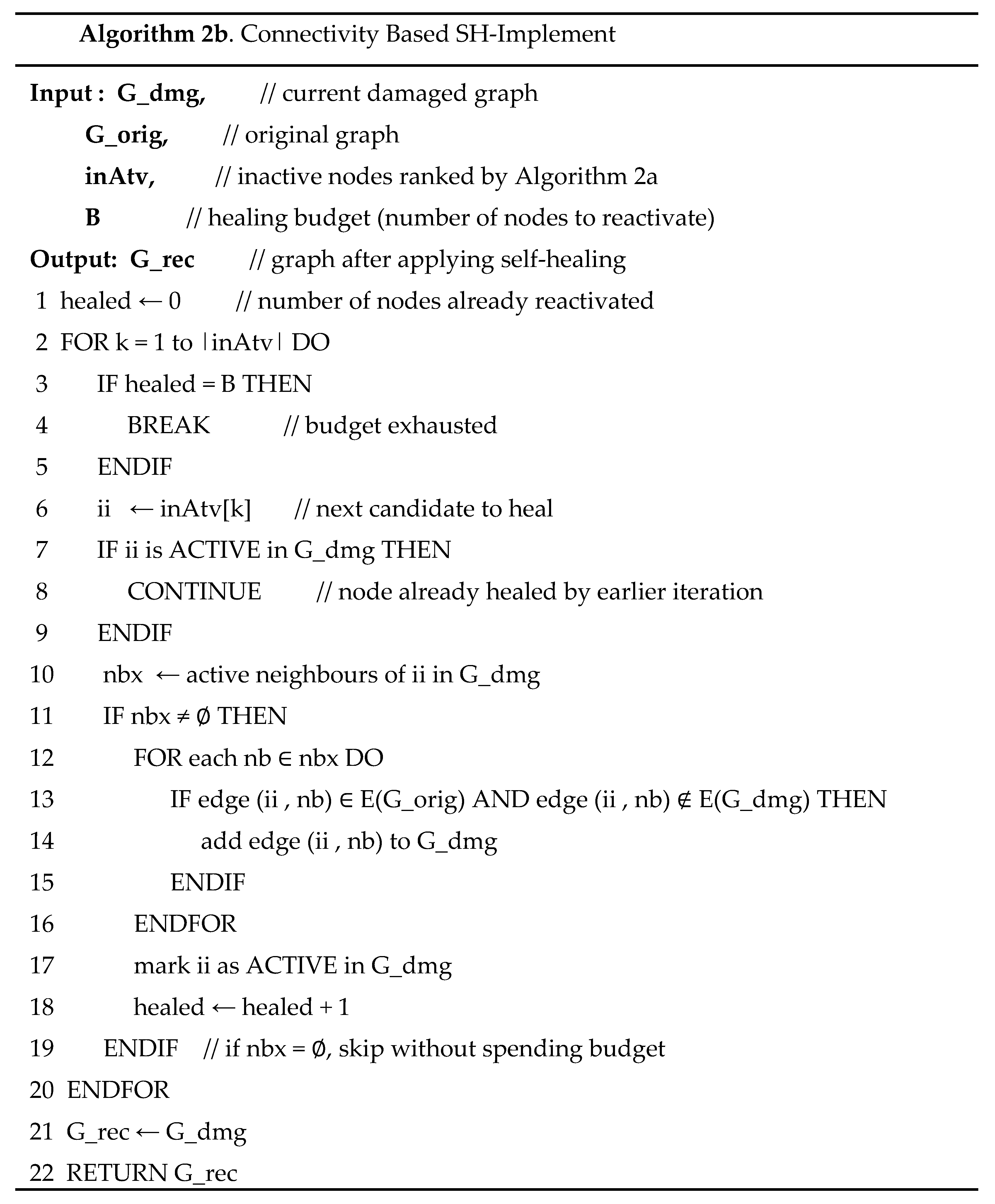
To restore functionality, we employ a self-healing (SH) scheme controlled by two parameters: Budget B is defined as the maximum number of inactive nodes that can be reactivated in a single time step and Triggering level T is defined as the fraction of nodes that must be inactive (with respect to the original network size) before healing begins.
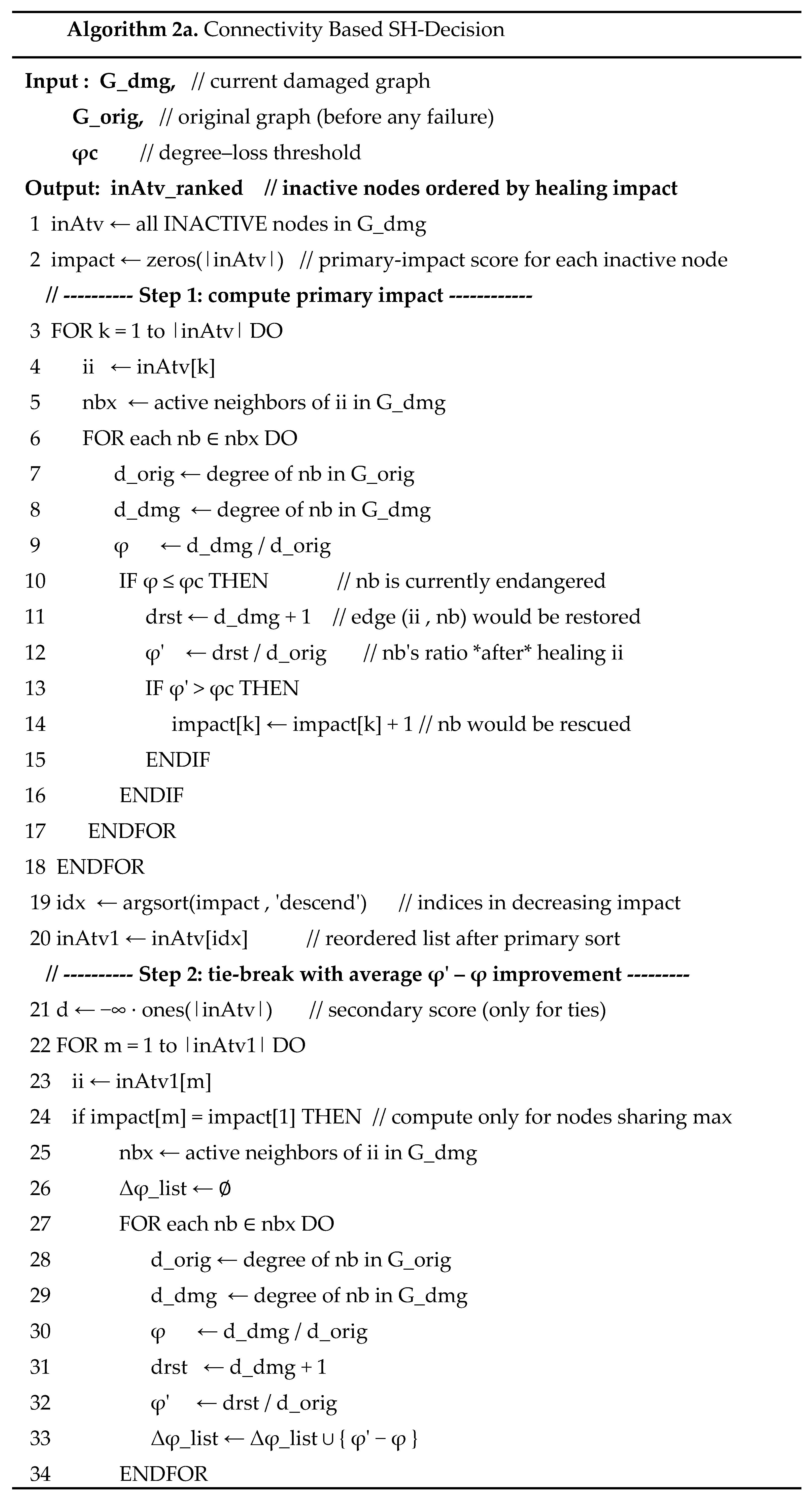
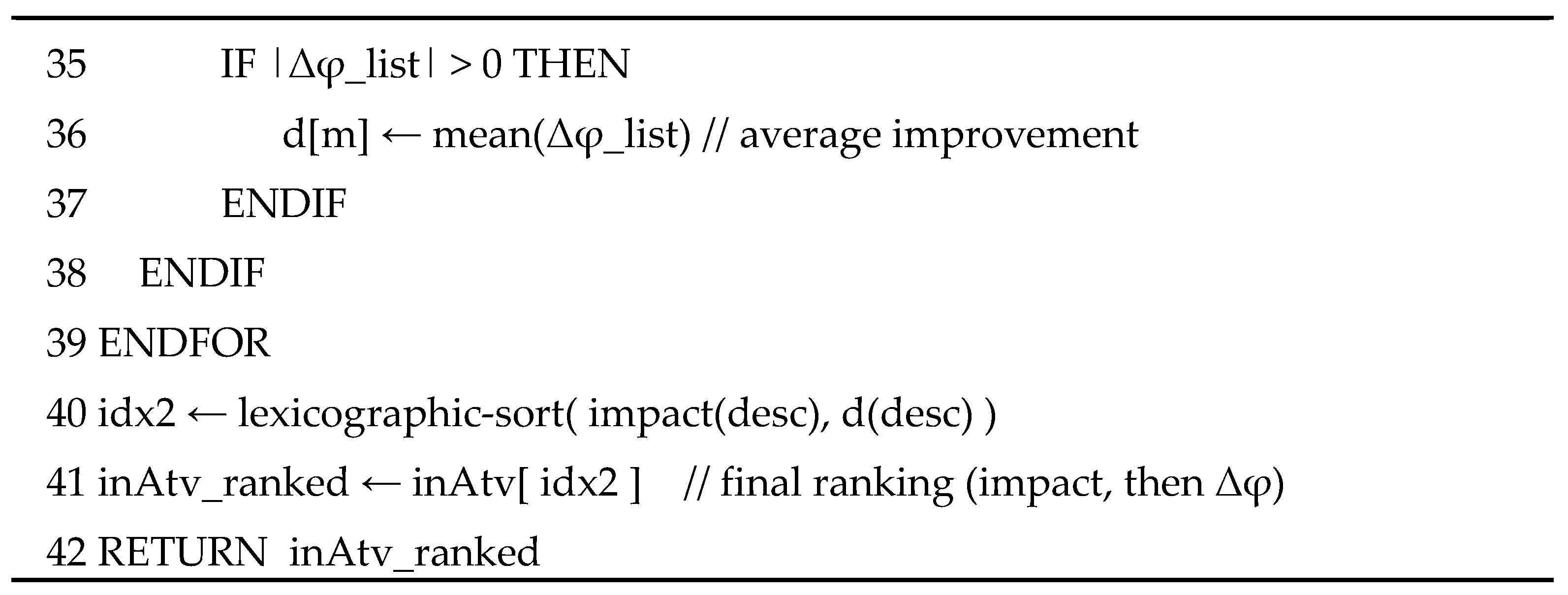
The healing stage comprises two sub-algorithms (Algorithms 2a and 2b):
- Step 1 – Decision (Algorithm 2a).
All inactive nodes that still have at least one active neighbor are identified. Each candidate node is assigned
- A primary impact: the number of active neighbors that would be saved if the node were reactivated (i.e., neighbors whose ratio would rise from <φc to ).
- A secondary impact: the average increase of those neighbors. Nodes are ranked first by primary impact and then, to break ties, by secondary impact.
- Step 2 – Implementation (Algorithm 2b).
Up to B highest-ranked inactive nodes are reactivated, and their original edges to currently active neighbors are restored, all within the current step.
The combined procedure iteratively applies failure propagation (Algorithm 1) and, once the trigger T is reached-healing (Algorithms 2a–2b) until no further changes occur.
In the connectivity-based model, failure propagation and self-healing are evaluated during the same global time step. Our implementation performs the failure routine first and then the healing routine; both updates are committed before the simulation advances to the next step, so the two processes are considered concurrent at the time-step level. Different relative “speeds” can be emulated by executing one routine multiple times in the same step (e.g., two failure passes followed by one healing pass to model faster failure dynamics).
2.2. Robustness and Resiliency Metrics
Robustness is quantified by the metric R, defined as
Because every node is active at , the denominator equals ; thus
Resiliency is evaluated with two complementary metrics:
- 1.
- Average Damage over a predefined time window :
Where is the fraction of nodes that are active at time .
- 2.
- 90% Recovery time, .
is the earliest time step at which at least 90% of the original nodes are active again.If the fraction of inactive nodes never falls below 10% within the simulation horizon, we set ; this indicates that the system is unable to recover to the 90% level.
These two metrics together capture both the depth of disruption and the speed of recovery .
2.3. Description of Data
Two real-world networks [28] are studied in this work. Figure 1 shows both datasets. The first is a U.S. airport network with 332 nodes, where each node represents an airport and each link indicates at least one direct flight between the corresponding airports. The second is a university email network with 1133 nodes; nodes represent email accounts and links indicate that at least one message was exchanged between the accounts. Figure 1a uses randomly assigned node coordinates for visual clarity and therefore does not reflect true airport locations. Figure 1c,d depict the degree histograms of the airport and email networks, respectively.
3. Results and Discussion
To probe the connectivity-based (CB) cascade model, we evaluate nine initial-attack fractions . For each we run 500 Monte-Carlo trials of Algorithms 1, 2a, and 2b under random attack, where the attacked nodes are selected uniformly at random. In the targeted-attack setting we also conduct 500 trials per , but in each trial the attacked set is chosen as the highest-degree hubs.
The remainder of this section is organized as follows: Section 3.1 presents robustness patterns R(α,φ) for the two real-world networks (U.S. airports, university e-mail), Section 3.2 analyses their resiliency metrics—average damage D and 90 % recovery time T90, and Section 3.3 examines the correlation between robustness and resiliency and discusses topological drivers of the observed trends.
3.1. Robustness Patterns
We quantify robustness with the metric R (Section II) and examine how it varies with the degree-loss threshold φ. Figure 2 displays R for the U.S. airport network ((a) random, (b) targeted) and for the university e-mail network ((c) random, (d) targeted). Each curve is the mean of 500 Monte-Carlo runs. The x-axis lists the initial-attack fraction a ∈ 0.1,…,0.9; nine threshold values φ=0.1,…,0.9 are plotted.
The four panels in Figure 2 reveal three consistent trends. First, targeted removal of high-degree hubs produces a markedly steeper drop in robustness R than an equivalent random failure, as can be seen by comparing panels (b) and (d) with panels (a) and (c). Second, increasing the degree-loss threshold invariably postpones secondary cascades: larger values preserve a greater fraction of nodes for every initial-attack fraction α, whereas low thresholds allow the network to collapse rapidly. Third, even under identical settings the U.S. airport graph retains a higher R than the university e-mail graph; this difference aligns with simple topological descriptors—most notably the airport network’s higher mean degree (12.8 versus 9.6) and its richer redundancy among hubs. Taken together, these results confirm that the connectivity-based model reproduces intuitive robustness dynamics and underscore the need for mitigation strategies that are tailored to a network’s specific connectivity profile.
3.2. Resiliency Patterns
The resiliency study focuses on the worst-case, targeted-attack scenario and uses the recovery-time metric T90—the number of simulation steps required for the network to return to at least 90 % active nodes. Figure 3 collects six panels that plot T90 against the healing budget B for three degree-loss thresholds and three triggering levels (T). In every panel the same qualitative tendencies appear but their quantitative expression differs between the two real-world graphs.
For the airport network the low-threshold case (Figure 3 a) is highly sensitive to the triggering level. When self-healing is postponed to the network may need more than 30 steps to regain 90 % functionality, whereas an early start at roughly halves the recovery time. As rises to 0.5 and 0.7 (Figs. 3 b and 3 c) the curves for the three triggering levels converge; once the threshold is high enough the cascade dies out quickly and T90 becomes almost independent of when healing begins. In every panel an initial increase of the budget yields marked reductions in T90, but beyond a critical budget the curves flatten, additional resources no longer accelerate recovery.
The e-mail network displays a different landscape. When the degree-loss threshold is low (, not shown) the network never reaches the 90 % mark and T90 is infinite for all and B. At (Figure 3 d) recovery becomes possible, yet the outcome remains extremely sensitive to : an early trigger restores the graph in fewer than ten steps for moderate budgets, whereas a late trigger can still leave T90 infinite at the same budget. Increasing to 0.6 (Figure 3 e) widens the range of budgets that guarantee finite recovery times, but the curves retain a pronounced separation by . A further increase to (Figure 3 f) paradoxically brings the system back to fragility—delayed healing never succeeds and even the earliest trigger needs large budgets to pull T90 below ten steps. Thus the e-mail graph shows a non-monotonic relation between robustness (as measured by ) and resiliency: intermediate thresholds perform best, whereas very low or very high thresholds lead to unrecoverable states.
Across all panels, increasing the budget always shortens recovery time until a saturation point is reached. For the airport graph that threshold is about at ; below it the system can oscillate between finite and infinite T90, while one incremental budget step above removes the bottleneck and halves T90. The same saturation effect appears in the e-mail graph, but it emerges at a lower budget fraction because that network is sparser—its nodes have fewer neighbors on average—so fewer reactivations are required to reconnect the giant component even though the graph contains more nodes overall.
These observations confirm that timely activation of self-healing and sufficient—but not excessive—budget allocation are the dominant levers of resiliency. The airport network profits from its denser, more redundant topology; once exceeds 0.5 its recovery speed is largely budget-limited and almost independent of the trigger. By contrast, the sparser e-mail network remains vulnerable to both late triggers and undersized budgets even at intermediate thresholds, while extreme thresholds () push it into regimes where recovery is impossible.
3.2.1. Budget Thresholds and Non-Linear Effects
A closer look at the airport data for illustrates how delicately recovery hinges on budget near a critical point. At the system still manages to heal, but slowly (T90=26). Reducing the budget by a single percentage point to drops the available resources below the minimum needed to reactivate key hubs; cascading failures therefore persist indefinitely and T90 diverges. Raising the budget again to supplies just enough edges to halt the cascade and T90 falls abruptly to 14. Such sharp transitions emphasize that resource planning must account for non-linear gains: small increments around the critical budget yield disproportionate improvements in resiliency.
3.2.2. Interplay Between Robustness and Resiliency
Because evolves during a cascade, robustness and resiliency are intertwined in a non-linear fashion. In the airport graph intermediate thresholds () strike an effective balance: the network can withstand initial damage and still recover under realistic budgets. Thresholds that are too low () or too high () push the system into failure modes that are hard to reverse, producing the same qualitative outcome—unbounded T90—for opposite structural reasons. The e-mail graph exhibits the same pattern but with much narrower safe intervals; it remains acutely sensitive to trigger times and budget sizes even at .
3.2.3. Implications
The combined analysis of robustness and resiliency shows that network topology dictates the feasible operating window. Dense, hub-rich infrastructures such as the airport network can tolerate delayed healing once is moderate, whereas sparse peer-to-peer structures such as the e-mail network demand both early intervention and carefully calibrated budgets. Beyond a network-specific saturation point additional resources bring diminishing returns, so precise allocation at or just above the critical budget is more effective than indiscriminate over-provisioning.
3.2.4. Average Damage as an Alternative Resiliency Metric
Because T90 cannot distinguish between partial-recovery and no-recovery trajectories that both end with an “infinite’’ time, we complement it with the average-damage measure, defined as the cumulative number of inactive nodes averaged over the observation window. Whereas T90 is a timing metric, average damage reflects the severity and persistence of cascade effects. Figure 4 plots this quantity for the two real-world graphs under the same targeted-attack setting used in Section 3.2; each panel pairs a degree-loss threshold with three triggering levels and sweeps the healing budget .
For the airport network the behavior changes markedly with . When average damage falls rapidly as soon as the budget rises above a few per-cent of the node count, but the final plateau depends on when recovery begins: early triggering () stabilizes below ten inactive nodes, an intermediate trigger () settles near a dozen, and a late trigger () remains much higher. At the intermediate threshold those three curves collapse onto one another; any trigger time is adequate provided the budget exceeds about five percent, emphasizing that resource availability rather than response time controls performance in this regime. Raising the threshold to eliminates temporal sensitivity: the three triggering levels collapse onto a single curve, so recovery performance depends almost exclusively on whether the budget exceeds the critical value of about twelve percent. A further increase to pushes the system beyond its tipping point; the cumulative damage stays above two hundred inactive nodes for all budgets and trigger times, revealing a paradox in which extreme structural robustness offers no practical resiliency because the initial loss is already too large.The e-mail network exhibits the same qualitative pattern but at different budget scales and with steeper transitions. At the curves are flat: average damage hovers around 191 for every B and T, confirming that the graph never recovers. Moving to introduces strong dependence on both control parameters. An early trigger combined with a budget above ten percent drives the average damage into double digits, but postponing recovery by only three time-steps causes the cumulative loss to exceed six hundred nodes unless the budget is very high. The threshold widens the window of successful operation; early and intermediate triggers converge once B passes fifteen percent, yet a late trigger remains ineffective. At the network again collapses irrespective of budget: the proportion of failures is simply too large to be reversed.
Across both graphs two conclusions emerge. First, average damage confirms the non-monotonic link between robustness and resiliency inferred from T90: thresholds that are either too low or too high leave the system in unrecoverable states, whereas an intermediate range () minimizes cumulative loss. Second, budget and trigger time trade off against each other only within that favorable range; outside it no realistic allocation can compensate for an untimely response or overwhelming initial damage. These findings suggest that effective recovery policy must identify the internal threshold regime where additional resources still translate into tangible resiliency gains and must prioritize rapid activation when the network operates near its tipping points.
3.3 Correlation Between Robustness and Resiliency (Airport Network, 10 % Initial Attack)
Figure 5 brings together six scatter plots obtained from the airport network after a fixed 10 % targeted attack. Each marker represents one of the seven degree-loss thresholds and is colored by the healing-budget fraction (blue 0.02, orange 0.05, grey 0.10, yellow 0.20). Robustness measured immediately after the attack is shown on the horizontal axis, while the vertical axis carries one of two resiliency indicators. Panels a, b, c plot the recovery time T90; panels d, e, f plot the cumulative average damage. All panels correspond to the three triggering thresholds .
3.3.1. Robustness Versus T90 (Panels a–c)
Early triggering (, panel a) produces an oblique cloud:high robustness combined with a tiny budget () still needs roughly thirty steps to reach 90 % activity, whereas ample funding () lets even fragile states () recover in fewer than ten steps. Panel b () shifts every point upward by two–three time-steps but preserves the same diagonal ordering, confirming that budget can compensate for limited robustness when the trigger is not too late. In contrast, panel c () shows nearly horizontal bands: after a long delay the cascade has spent itself and T90 depends almost solely on budget, with robustness contributing little additional leverage.
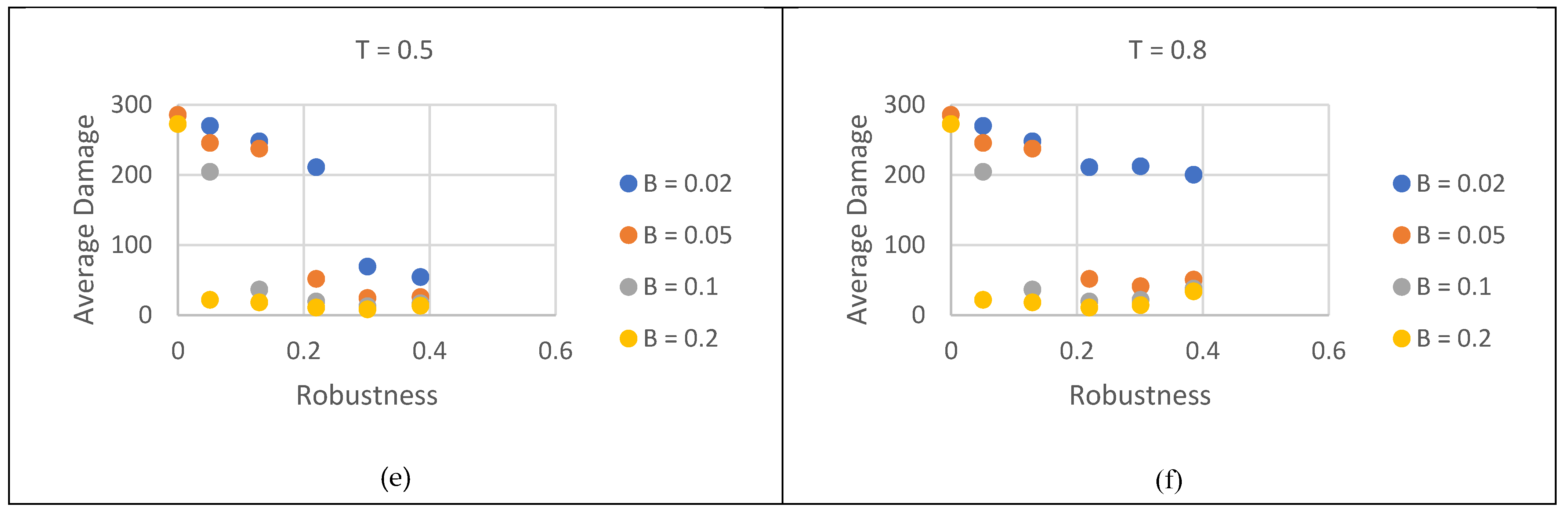
3.3.2. Robustness Versus Average Damage (Panels d–f)
The average-damage panels trace the same interplay in terms of damage magnitude. With a prompt trigger (panel d) cumulative loss stays below fifty nodes whenever either robustness or budget is high, but exceeds 250 nodes when both are low. A moderate delay (panel e) widens the damage gap between low and high budgets, especially for fragile states. Under the late trigger (panel f) damage stratifies almost perfectly by budget: blue markers () cluster near 200 inactive nodes regardless of robustness, while yellow markers () cluster below fifty nodes, indicating that once intervention is late, budget dominates and robustness ceases to influence cumulative loss.
3.3.3. Interpretation and Design Implications
Taken together, the six panels show that robustness and resiliency are related but distinct. A configuration that survives the initial attack well can still recover slowly or sustain heavy loss if resources are tight, whereas a fragile configuration can rebound rapidly given timely and ample funding. Budget and trigger time trade off only when intervention is early; once healing is substantially delayed, increasing robustness adds little benefit. Empirically, the relationship can be approximated by a multiplicative form with β≈1and a weak robustness factor when is large—underscoring that prompt, well-funded self-healing is more effective than structural hardening alone.
4. Conclusion
This paper developed and analyzed a concurrent failure-and-healing framework for connectivity-based cascades on real-world networks. The model couples a link-breaking failure rule—activated when a node’s active-neighbor ratio drops below a threshold—with a distributed self-healing rule that is governed by a triggering level and a budget . By sweeping the four-dimensional parameter space () on a U.S. airport graph and a university e-mail graph we obtained three main results.
- 1.
- Distinct robustness regimes. Robustness declines smoothly under random attack but collapses abruptly under targeted hub removal; increasing mitigates both effects, although the airport network remains consistently more robust owing to its higher mean degree and redundant hub set.
- 2.
- Budget-trigger trade-off in resiliency. Early activation with a modest budget outperforms late activation with a larger budget. A critical “saturation” budget exists—about 12 % of nodes for the airport graph and 10 % for the e-mail graph—beyond which additional resources yield only marginal gains in T90 and average damage.
- 3.
- Weak correlation between robustness and resiliency. Scatter-plot analysis showed that configurations with high robustness can still recover slowly when under-funded, while low-robustness configurations can rebound rapidly if healing is timely and well resourced. A simple multiplicative fit (with) summarizes this interaction.
4.1. Design Implications
Structural hardening alone is insufficient. Ensuring prompt, adequately funded self-healing is equally, and sometimes more effective than raising the robustness threshold. Resource allocation policies should therefore target the critical budget that precedes saturation, and detection systems should minimize trigger delays.
4.2. Limitations and Future Work
We studied static budgets and single-layer networks. Extending the framework to adaptive budgets, multi-layer interdependencies and spatially constrained repair crews would bring the analysis closer to operational practice. Incorporating load-based dynamics in the same concurrent setting is another important step, as is validating the model on time-stamped failure-and-repair data from real infrastructures.
By quantifying both robustness and resiliency, and their subtle interplay, this work provides a foundation for recovery-aware design of complex networked systems.
Abbreviations
The following abbreviations are used in this manuscript:
| G | Current graph |
| Gdmg | Graph after the cascading-failure phase |
| Grec | Graph returned after the healing phase |
| N | List (or count) of currently functional nodes |
| E | List of currently present edges |
| active | Vector of original degrees |
| fail | Vector of current degrees |
| φc | Degree-loss threshold that triggers node failure |
| φ | Ratio current degrees/ original degrees for a node |
| needrmv | Boolean vector marking nodes with φ<φc |
| cand | Set of nodes that newly fail in the current sweep |
| idx | Indices of nodes sorted by descending original degree |
| rmodes | Initial attack set (random or targeted) |
| inAtv | List of inactive nodes that still have ≥1 active neighbor |
| impact | Primary-impact score: # of endangered neighbors rescued by healing a candidate node |
| d | Secondary score: mean improvement (φ′−φ) for neighbors rescued by that candidate |
| nbx | Set of active neighbors of a specific inactive node |
| d_orig | Original degree of a neighbor |
| d_dmg | Current degree of a neighbor |
| drst | Degree neighbor would have after edge restoration |
| φ′ | Updated degree ratio after hypothetical healing |
| idx2 | Permutation that ranks inAtv lexicographically by primary and secondary impact |
| inAtv_ranked | Final ranked list of inactive nodes to heal |
| B | Healing-budget cap: max # of nodes reactivated in a step |
| healed | Counter for how many nodes have been reactivated so far |
| nb | Individual active neighbor |
| T | Triggering level: fraction of inactive nodes that starts healing |
References
- J. M. Carlson and J. Doyle, “Complexity and robustness,” Proc. Natl. Acad. Sci., vol. 99, no. suppl_1, pp. 2538–2545, Feb. 2002. [CrossRef]
- “The Resilience of Networked Infrastructure Systems | Systems Research Series.” Accessed: May 24, 2025. [Online]. Available: https://www.worldscientific.com/worldscibooks/10.1142/8741.
- Z. Huang, C. Wang, A. Nayak, and I. Stojmenovic, “Small Cluster in Cyber Physical Systems: Network Topology, Interdependence and Cascading Failures,” IEEE Trans. Parallel Distrib. Syst., vol. 26, no. 8, pp. 2340–2351, Aug. 2015. [CrossRef]
- J. Zhang, E. Yeh, and E. Modiano, “Robustness of Interdependent Random Geometric Networks,” Jun. 04, 2018, arXiv: arXiv:1709.03032. [CrossRef]
- C. Sergiou, M. Lestas, P. Antoniou, C. Liaskos, and A. Pitsillides, “Complex Systems: A Communication Networks Perspective Towards 6G,” IEEE Access, vol. 8, pp. 89007–89030, 2020. [CrossRef]
- S. Pahwa, C. Scoglio, and A. Scala, “Abruptness of Cascade Failures in Power Grids,” Sci. Rep., vol. 4, no. 1, p. 3694, Jan. 2014. [CrossRef]
- B. Schäfer, D. Witthaut, M. Timme, and V. Latora, “Dynamically induced cascading failures in power grids,” Nat. Commun., vol. 9, no. 1, p. 1975, May 2018. [CrossRef]
- Y. Wang, B. Chen, X. Chen, and X. Gao, “Cascading Failure Model for Command and Control Networks Based on an m-Order Adjacency Matrix,” Mob. Inf. Syst., vol. 2018, p. e6404136, Dec. 2018. [CrossRef]
- W. A. Aqqad and X. Zhang, “Modeling command and control systems in wildfire management: characterization of and design for resiliency,” in 2021 IEEE International Symposium on Technologies for Homeland Security (HST), Nov. 2021, pp. 1–5. [CrossRef]
- Y. Li, D. Duan, G. Hu, and Z. Lu, “Discovering Hidden Group in Financial Transaction Network Using Hidden Markov Model and Genetic Algorithm,” in 2009 Sixth International Conference on Fuzzy Systems and Knowledge Discovery, Aug. 2009, pp. 253–258. [CrossRef]
- D. J. Watts, “A simple model of global cascades on random networks,” Proc. Natl. Acad. Sci., vol. 99, no. 9, pp. 5766–5771, Apr. 2002. [CrossRef]
- C. Stegehuis, R. van der Hofstad, and J. S. H. van Leeuwaarden, “Epidemic spreading on complex networks with community structures,” Sci. Rep., vol. 6, no. 1, p. 29748, Jul. 2016. [CrossRef]
- A. E. Motter and Y.-C. Lai, “Cascade-based attacks on complex networks,” Phys. Rev. E, vol. 66, no. 6, p. 065102, Dec. 2002. [CrossRef]
- X. Huang, J. Gao, S. V. Buldyrev, S. Havlin, and H. E. Stanley, “Robustness of interdependent networks under targeted attack,” Phys. Rev. E, vol. 83, no. 6, p. 065101, Jun. 2011. [CrossRef]
- X. Huang, S. Shao, H. Wang, S. V. Buldyrev, S. Havlin, and H. E. Stanley, “The robustness of interdependent clustered networks,” EPL Europhys. Lett., vol. 101, no. 1, p. 18002, Jan. 2013. [CrossRef]
- X. Yuan, S. Shao, H. E. Stanley, and S. Havlin, “How breadth of degree distribution influences network robustness: Comparing localized and random attacks,” Phys. Rev. E, vol. 92, no. 3, p. 032122, Sep. 2015. [CrossRef]
- S. Chattopadhyay, H. Dai, D. Y. Eun, and S. Hosseinalipour, “Designing Optimal Interlink Patterns to Maximize Robustness of Interdependent Networks Against Cascading Failures,” IEEE Trans. Commun., vol. 65, no. 9, pp. 3847–3862, Sep. 2017. [CrossRef]
- A. E. Motter, “Cascade control and defense in complex networks,” Phys. Rev. Lett., vol. 93, no. 9, p. 098701, Aug. 2004. [CrossRef]
- L. K. Gallos and N. H. Fefferman, “Simple and efficient self-healing strategy for damaged complex networks,” Phys. Rev. E, vol. 92, no. 5, p. 052806, Nov. 2015. [CrossRef]
- W. Quattrociocchi, G. Caldarelli, and A. Scala, “Self-Healing Networks: Redundancy and Structure,” PLOS ONE, vol. 9, no. 2, p. e87986, Feb. 2014. [CrossRef]
- T. Wang, J. Zhang, X. Sun, and S. Wandelt, “Network repair based on community structure,” Europhys. Lett., vol. 118, no. 6, p. 68005, Sep. 2017. [CrossRef]
- C. Liu, D. Li, B. Fu, S. Yang, Y. Wang, and G. Lu, “Modeling of self-healing against cascading overload failures in complex networks,” Europhys. Lett., vol. 107, no. 6, p. 68003, Sep. 2014. [CrossRef]
- S. I. Mari, Y. H. Lee, and M. S. Memon, “Sustainable and Resilient Supply Chain Network Design under Disruption Risks,” Sustainability, vol. 6, no. 10, Art. no. 10, Oct. 2014. [CrossRef]
- K. A. T. H. L. E. E. N. T. I. E. R. N. E. Y. A. N. D. M. I. C. H. E. L. B. R, “Conceptualizing and Measuring Resilience a Key to Disaster Loss Reduction,” Accessed: May 24, 2025. [Online]. Available: https://www.semanticscholar.org/paper/Conceptualizing-and-Measuring-Resilience-a-Key-to-K.ATHLEENTIERNEYANDMICHELB/a6a6444d31810223d641cfd900c680c396ef3bec.
- G. Pumpuni-Lenss, T. Blackburn, and A. Garstenauer, “Resilience in Complex Systems: An Agent-Based Approach,” Syst. Eng., vol. 20, no. 2, pp. 158–172, 2017. [CrossRef]
- R. A. R. others Nesreen K. Ahmed, and, “USAir97 | Miscellaneous Networks | Network Repository,” Network Data Repository. Accessed: May 25, 2025. [Online]. Available: https://networkrepository.com/USAir97.php.
Figure 1.
(a) A US airports network consisting of 332 nodes. (b) A university Email network consisting of 1133 nodes. (c) A degree histogram of the US airports network. (d) A degree histogram of the university email network.
Figure 1.
(a) A US airports network consisting of 332 nodes. (b) A university Email network consisting of 1133 nodes. (c) A degree histogram of the US airports network. (d) A degree histogram of the university email network.
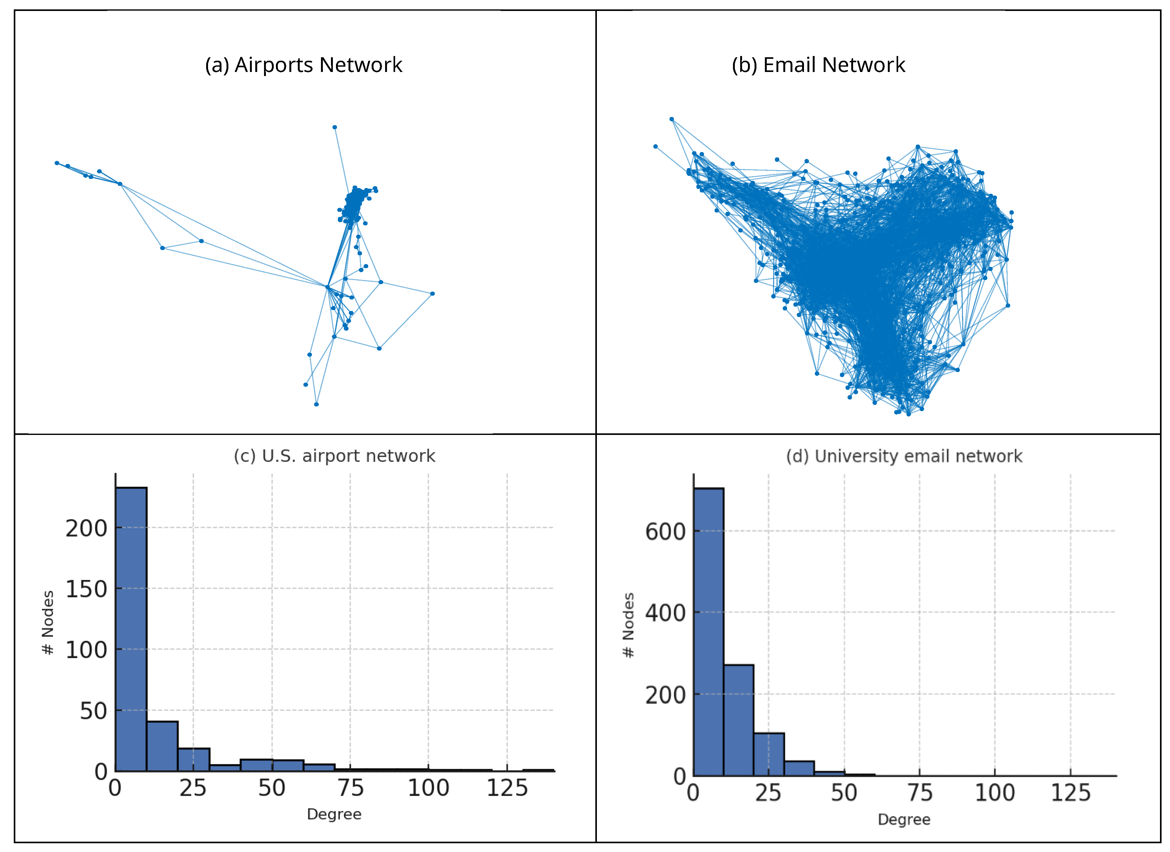
Figure 2.
Robustness R as a function of initial-attack fraction α and degree-loss threshold φ: (a) U.S. airport network, random attack; (b) U.S. airport network, targeted attack; (c) university e-mail network, random attack; (d) university e-mail network, targeted attack. Curves show the mean of 500 simulations. Variance across 500 Monte-Carlo runs is below ±0.01 for all curves; error bands are therefore omitted for visual clarity. Targeted attacks remove the top-k hubs (highest degree) at each α, leading to markedly lower robustness than random attacks.
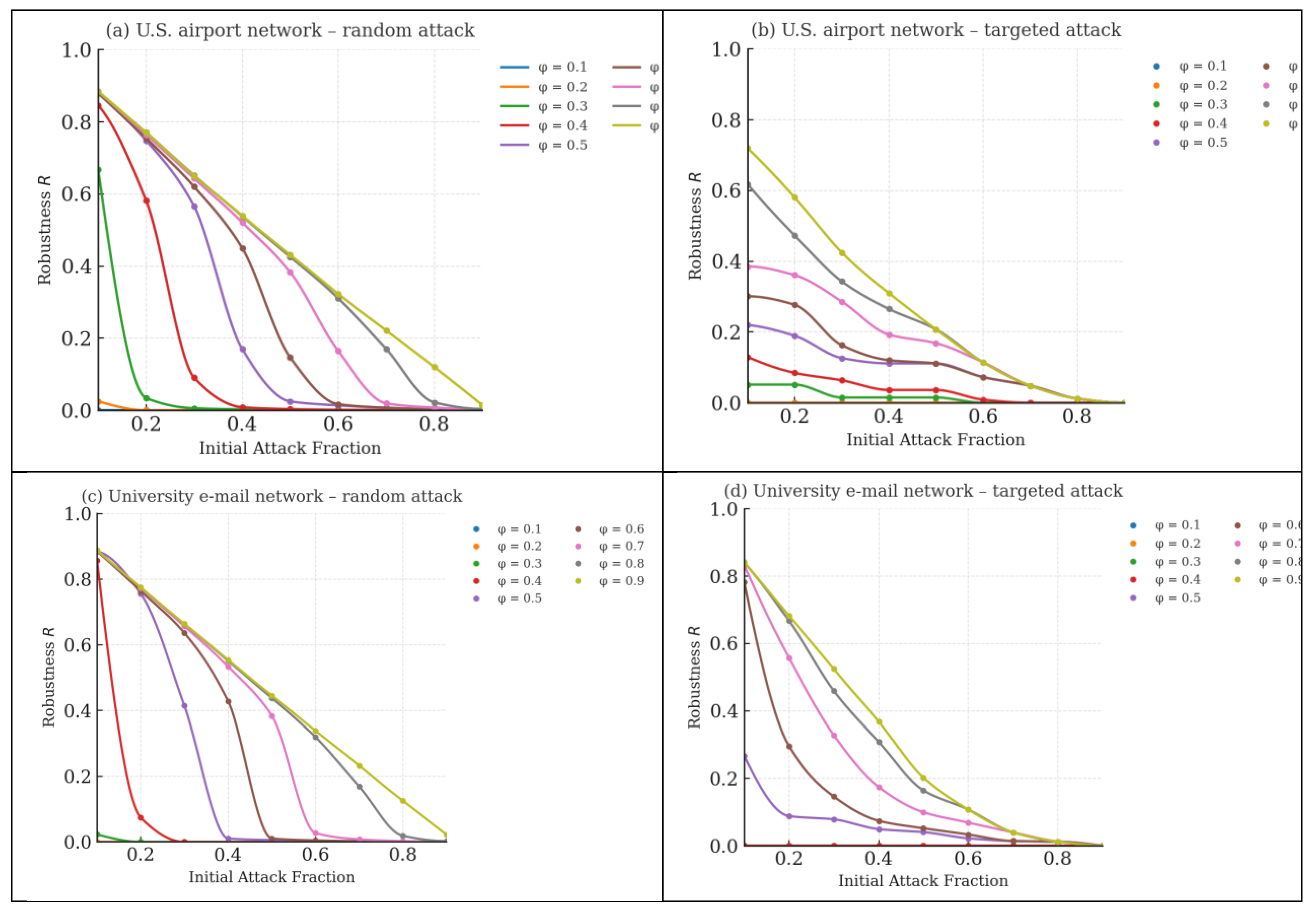
Figure 3.
Ninety-percent recovery time T90 as a function of the healing budget for three triggering levels . Panels (a)–(c) correspond to the U.S. airport network at degree-loss thresholds ; panels (d)–(f) show the university e-mail network at . Solid, dashed and dash-dotted lines represent the three T-values, and curves terminate at T90=∞ where recovery never reaches the 90 % level. In panels (b) and (c) the three T-curves are numerically identical and therefore appear as a single line.
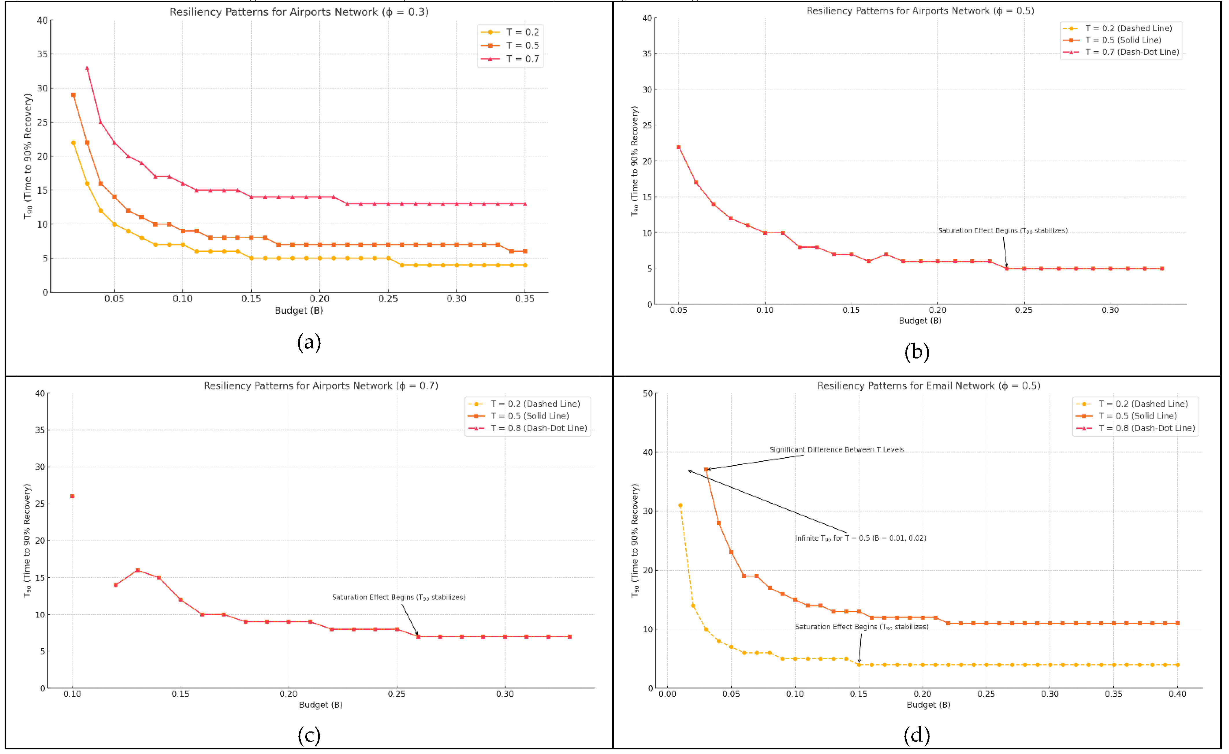
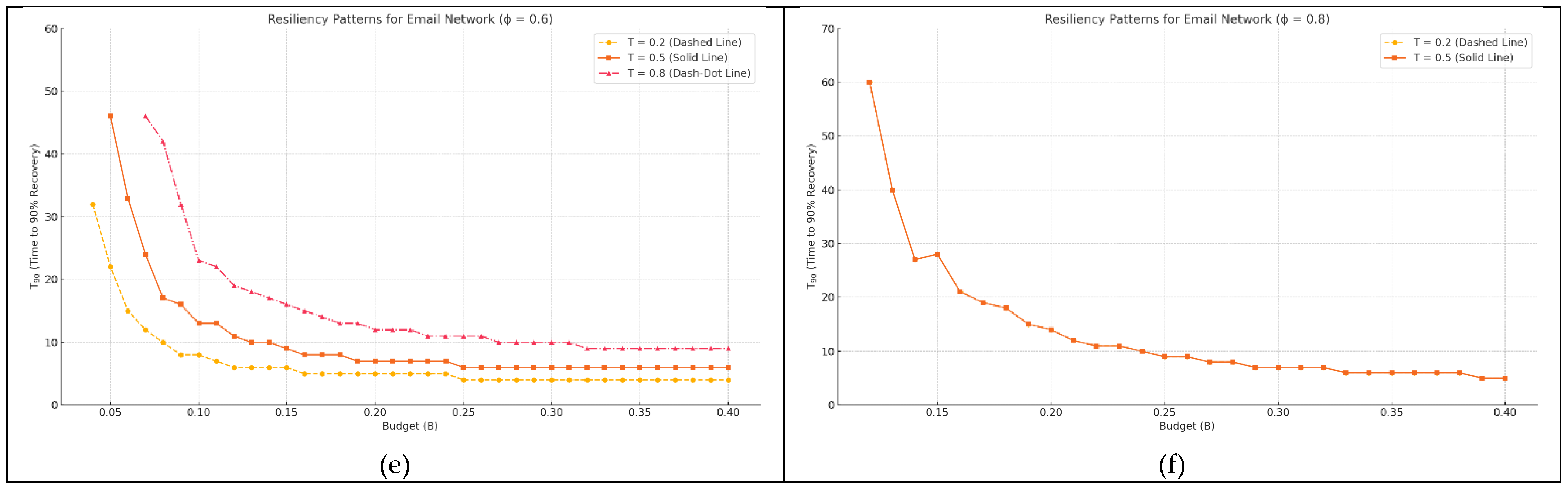
Figure 4.
Average damage as a function of healing budget B for three triggering levels (dashed), (solid) and (dash-dot). Panels (a)–(c) correspond to the U.S. airport network with ; panels (d)–(f) show the university e-mail network with . Curves that coincide—for example all three triggers in panel (b) and panel (d)—are plotted once; identical legends are retained for completeness.
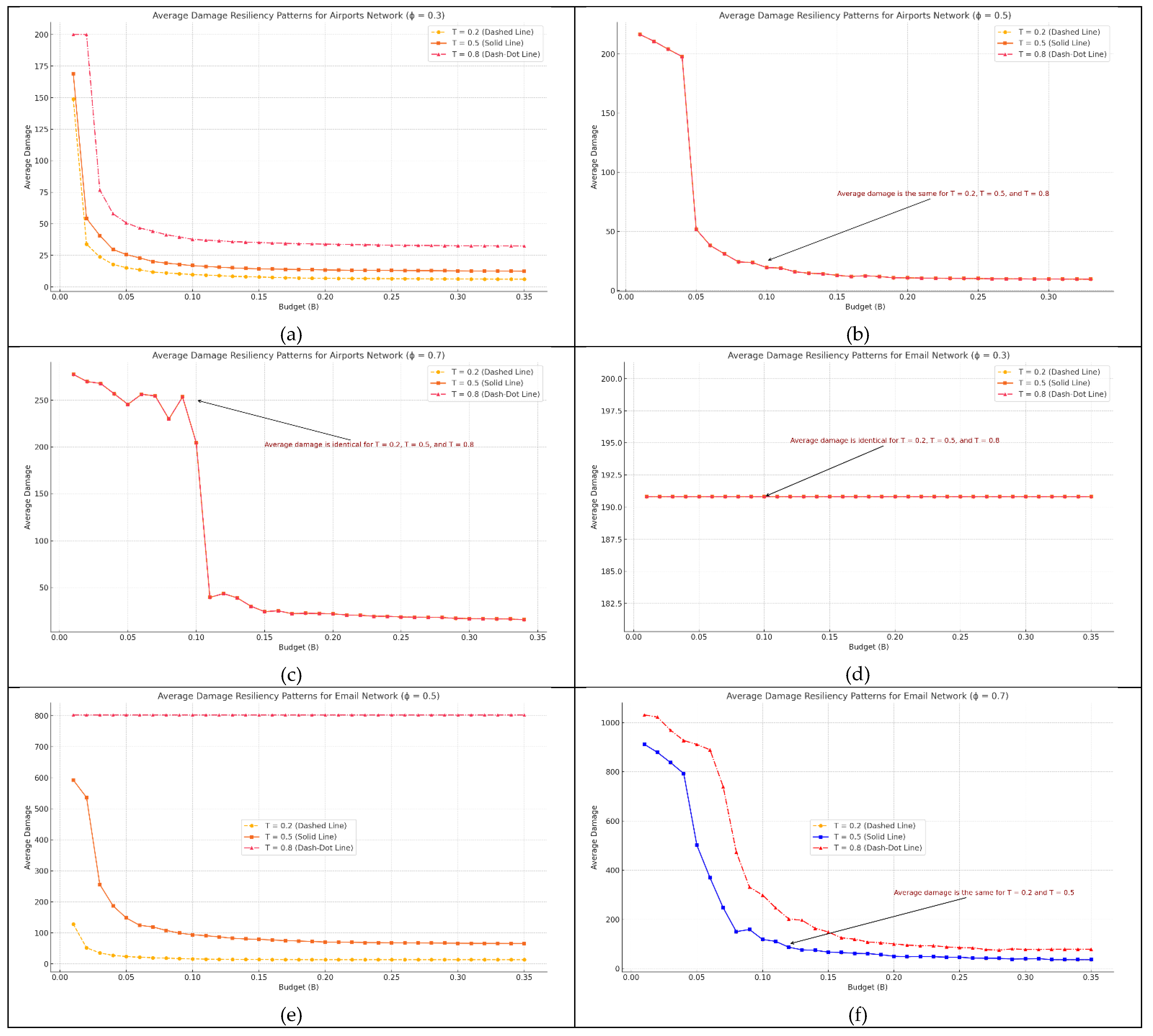
Figure 5.
Correlation between robustness and two resiliency measures for the airport network under a 10 % targeted attack. (a)–(c) T90 as a function of robustness for triggering thresholds . (d)–(f) Cumulative average damage for the same three triggering levels. Marker colors denote budget fractions (blue), (orange), (grey), and (yellow). Each point arises from one degree-loss threshold . The scatter illustrates that robustness alone does not determine resiliency: high-states can recover slowly when is small, whereas low- states rebound quickly if the budget and trigger are favorable.

Disclaimer/Publisher’s Note: The statements, opinions and data contained in all publications are solely those of the individual author(s) and contributor(s) and not of MDPI and/or the editor(s). MDPI and/or the editor(s) disclaim responsibility for any injury to people or property resulting from any ideas, methods, instructions or products referred to in the content. |
© 2025 by the authors. Licensee MDPI, Basel, Switzerland. This article is an open access article distributed under the terms and conditions of the Creative Commons Attribution (CC BY) license (http://creativecommons.org/licenses/by/4.0/).
Copyright: This open access article is published under a Creative Commons CC BY 4.0 license, which permit the free download, distribution, and reuse, provided that the author and preprint are cited in any reuse.


