
Submitted:
26 May 2025
Posted:
26 May 2025
You are already at the latest version
Abstract
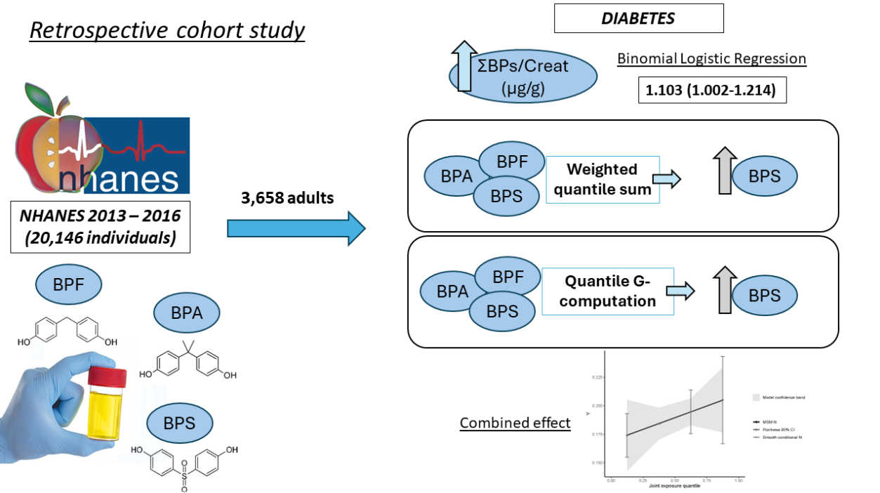
Humanity lives in a new era marked by the ubiquitous presence of plastics worldwide. Recent figures highlight continuous growth in plastic production and usage, a trend paralleled by the rise in chronic diseases like diabetes. The multifactorial nature of these diseases suggests that environmental exposure, notably to bisphenol A (BPA), could be a contributing factor. This study investigates the potential correlation between emerging BPA substitutes, bisphenol S and F (BPS and BPF), and diabetes in a cohort of the general adult population. Findings reveal a positive association between combined bisphenols (BPs) and glycated haemoglobin (Hb1Ac), with binomial logistic regression demonstrating an odds ratio (OR) of 1.103 (1.002-1.214) between BP levels corrected for creatinine (crucial due to glomerular filtration variations) and diabetes. Advanced statistical methods, including Weighted Quantile Sum (WQS) and quantile G-computation analysis, show a combined positive effect on diabetes, glucose levels, and Hb1Ac. Individual effect analysis identifies BPS as a significant monomer warranting attention in future diabetes-related research. Ultimately, replacing BPA with new molecules like BPS or BPF may pose a greater risk in the context of diabetes.
Keywords:
Endocrine Disruptors
; Diabetes
; Bisphenol S
; Bisphenol F
; Bisphenol A
; Retrospective Cohort Study
1. Introduction
The contemporary era, often referred to as the “Anthropocene” or the “Plastic Age”, owes its name to the extremely close relationship that humans have developed with plastic polymers [1]. Plastics have become a fundamental element of modern industry because of their countless applications and cost-effectiveness, but they pose a major threat to the environment and to global population health. The centrality of plastic in modern society extends from its use in food packaging to clothing, exposing us directly to xenobiotic compounds [2,3,4]. At the core of this plastic surge is bisphenol A (BPA), a monomer and endocrine disruptor found in epoxy resins and polycarbonates, enhancing the physical properties of diverse polymers [5].
Over time, plastic production has surged dramatically, reaching 368 million tons in 2019 [6], with projections indicating a doubling within the next two decades [7]. This surge, coupled with challenges in waste management and the perpetual cycle of polymer production and recycling, raises concerns about potential far-reaching impacts across various trophic levels [8], posing a substantial threat of chronic human exposure. Recent research unequivocally confirms the widespread presence of plastic monomers, including the emerging bisphenol S and F monomers (BPS and BPF), in water bodies, soil and atmosphere worldwide. [4,9,10].
Parallel to the increased production and use of this class of monomers has been a significant increase in the incidence of diabetes worldwide. Diabetes mellitus (DM) emerges as a prominent global health crisis in the 21st century [11], with a substantial increase in prevalence over recent decades. Back in 1980, approximately 108 million adults aged 20–79 years were affected. Presently, DM affects 10.5% of the global population (536 million individuals), and projections anticipate a potential rise to 12.2% by 2045 (783.2 million) [12]. The risk factors associated with DM encompass a broad spectrum of environmental and genetic elements, including variables such as age, weight, diet, and smoking [13]. This prompts a consideration of the plausible role that environmental pollutants might play in the development or progression of the disease. Existing literature offers insights into this intriguing intersection. Studies suggest a conceivable relationship between DM and environmental pollutants, providing a nuanced perspective on the complex factors contributing to this escalating health challenge [14].
In this regard, a recent meta-analysis demonstrated the need for further analysis of new bisphenols used in industry as substitutes for BPA in view of the increasingly restrictive regulations being promoted in different countries [15]. The results of the meta-analysis showed a statistically significant positive association only with BPS. Nevertheless, it is evident that in the real world, outside the regulated laboratory setting, co-exposure to bisphenols does occur, as demonstrated in human cohorts that quantify the presence of a mixture of bisphenols in urine [16]. However, the paucity of publications studying the possible combined effect of these monomers in the context of DM is striking. In other variations of DM such as gestational DM (GDM), recent research shows that BPS and BPF could be potential risk factors for its development [17,18].
Consequently, the present work aims to analyze the possible combined effect of the mixture of the three most relevant bisphenols in modern industry with the risk of DM in one of the largest global cohorts analyzing urinary bisphenols, the “National Health and Nutrition Examination Survey” (NHANES) cohort. Thus, using correlations, logistic regressions, Weighted quartile sum and quantile G-computational analysis, the possible relationship between combined bisphenol exposure and DM in adults will be explored.
2. Materials and Methods
2.1. Data ExtRaction fRom the NHANES CohoRt
The NHANES cohort databases from all years in which urinary bisphenol levels were quantified were utilized. Currently, the 2013-2014 and 2015-2016 cohorts have data on the quantification of urinary BPA, BPF and BPS. All data are accessible on the official website of the Centers for Disease Control and Prevention [19] (accessed on november 13, 2023). After consolidating and organizing the data by patient code, a total of 20,146 subjects were obtained. The data were then filtered based on subjects aged 18 and above (adults), urinary bisphenol values, and urinary creatinine values, resulting in a total of 3,699 subjects included in the database for analysis. The study population was further subdivided based on the pathology of interest (diabetes), and participants with data on all relevant covariates (to be detailed later) were selected, yielding 3,658 study subjects (2,965 non-diabetics and 693 diabetics) (Figure 1). Individuals with physician-diagnosed diabetes, as well as those with fasting glucose values ≥ 126 mg/dl or haemoglobin A1c ≥ 6.5%, were included in the diabetic group [20].
2.2. Combined URinaRy Bisphenol ExposuRe Study
In the combined study of urinary bisphenols, we first used an approach based on the analysis of the sum of these phenolic compounds. Initially, analyses were conducted based on “Unsupervised summary scores or USS,” as outlined by Li et al. [21]. This involved calculating the molar sum of bisphenols (ΣBPs/Mol) by dividing the concentration of each metabolite by its respective molecular weight and subsequently summing them up:
In the subsequent step, the total concentration of bisphenols, adjusted by the urinary creatinine value (Creat), was employed to mitigate potential result discrepancies stemming from variations in the glomerular filtration capacity among individual study subjects (ΣBPs/Creat).
The quantification of bisphenols was conducted using an online solid-phase extraction coupled with high-performance liquid chromatography and tandem mass spectrometry (online SPE-HPLC-Isotope dilution-MS/MS) method. The respective detection limits were 0.2, 0.2, and 0.1 for BPA, BPF, and BPS. For more information on the protocols, refer to the NHANES website [22,23].
Basic descriptive statistics were conducted to analyze the variables of interest within each of the pathological subgroups, as well as in the bisphenol’s quartiles. Quantitative variables were reported as the arithmetic mean (standard deviation), AM (SD), or as the geometric mean (95% confidence interval), GM (95% CI), depending on their normality. Descriptive statistical analysis, comparative analysis, and graphical representation were performed using GraphPad Prism 7.0 software (GraphPad Software Inc., San Diego, CA, USA). The distribution of data was assessed using the D’Agostino-Pearson, Shapiro-Wilk, and Kolmogorov-Smirnov normality tests. Subsequently, either the T-student or Mann-Whitney test was employed for the comparative analysis of two variables. For three or more variables, one-way ANOVA or Kruskal-Wallis, followed by a Bonferroni or Dunn’s test, was carried out. T-test and Fisher’s exact test was used for the analysis of dichotomous variables in descriptive statistics. The p-values in the figures and tables correspond to the post hoc test, with a significance level set at p < 0.05.
Next, Pearson correlation analysis was employed to assess potential relationships between urinary bisphenols and quantitative variables such as age, body mass index, cotinine levels, serum glucose, and glycosylated haemoglobin. In the subsequent step, a study model involving binomial and multinomial logistic regression was implemented. The aim of the logistic regression analysis was to identify patterns that could reveal potential associations between the pathological subgroups and the composite of urinary bisphenols, considering the multifactorial origin of the study pathologies. Subsequently, each analysis was conducted in three distinct manners: first, individually (1); second, adjusted for age, gender, and Body Mass Index (BMI) (2); and third, adjusted for (2) + race/ethnicity, poverty-income ratio, hypertension, dyslipidemia, and smoking (3) (inclusion of anthropometric and demographic variables as per relevant literature [21,24,25]). Individuals classified as hypertensive comprised those diagnosed by a healthcare professional and those with systolic pressure ≥ 140 mmHg or diastolic pressure ≥ 90 mmHg. The category of patients with dyslipidemia included those diagnosed with cholesterol disorders or those with fasting total cholesterol levels ≥ 240 mg/dL[26]. Regarding smoking, individuals were included if they answered affirmatively to the question “have you smoked more than 100 cigarettes in your life?” or if they had serum cotinine values exceeding 10 mg/dL [27]. Log-transformation of urinary concentrations of bisphenol metabolites was applied to achieve normalized distributions. The Cochran q test and regression models were performed using IBM SPSS Statistics for Windows software, version 27 (IBM Corp, Armonk, NY, USA).
Following this, the weighted quantile sum (WQS) was constructed utilizing the R package “gWQS” [28] to investigate associations between the exposures and the outcome, concurrently providing a comprehensive summary of the intricate exposure to the particular mixture of interest [29,30]. In essence, WQS regression condenses the overall exposure to the mixture by calculating a singular weighted index, considering the individual contribution of each component through assigned weights [31]. In the combined analysis, the individual value of each of the bisphenols corrected by the urinary creatinine value (BPA/creat, BPS/creat and BPF/creat) was entered.
Subsequently, a quantile G-computation model was executed using the R package “qgcomp” [32] to estimate the collective impact of the bisphenols mixture on Heart Disease. The QG-comp method evaluates the effect of the bisphenol mixture on the outcome by measuring the change in outcome for each quantile increase in the concentration of all bisphenols in the mixture. Furthermore, it calculates the relative contribution of each bisphenol to the overall effect, discerning whether it has a positive or negative direction. The estimated overall mixture effect, denoted as ψ, signifies the alteration in the outcome associated with a quantile increase in the concentration of all bisphenols in the mixture. In essence, ψ captures the joint effect of all bisphenols in the mixture on the outcome, allowing for an assessment of the overall impact of the bisphenol mixture on the outcome of interest.
3. Results
The initial stage in the statistical analysis of subpopulations within the NHANES cohort involved conducting descriptive statistics. As illustrated in Table 1, most of the study covariates employed to adjust the statistical models exhibited noteworthy differences between individuals with and without the pathology of interest. Subjects in the diabetic category were older and had a higher BMI, as is logical in this pathology. In addition, the pathological subgroup presented a higher percentage of subjects with hypertension, dyslipidemia and smokers. With respect to urinary bisphenol levels, there were significant differences between the creatinine-corrected values, while the USS showed no differences between groups. Finally, ethnic differences were also observed, with an increase in the percentage of Mexican American, other Hispanic and non-Hispanic black subjects among healthy and diabetic subjects, as well as a lower percentage of non-Hispanic white diabetics compared to the non-diabetic group.
The subsequent comparative analysis of the BPmix quartiles (Table 2 and Table 3) revealed intriguing ethnic differences, particularly pronounced in values normalized by molecular weight (ΣBPs/Mol). Notably, a negative trend was observed in the ‘Non-Hispanic White’ population, contrasting with a reverse trend in the ‘Non-Hispanic Black’ population. Interestingly, the analysis did not reveal significant results regarding diabetes in either of the two approaches used with corrected bisphenol values. However, ΣBPs/Creat exhibited a significant increase in hypertensive and smoking subjects, and, intriguingly, a higher percentage of women in Q4 compared to Q1. Furthermore, in both approaches, a significant decrease in the Poverty-Income Ratio is observed, and in the case of ΣBPs/Mol, there is an increase in BMI.
The next step involved Pearson correlation analysis between quantitative variables of interest, such as parameters related to diabetes (Glucose, glycated haemoglobin), as well as cholesterol and cotinine. In this case, the results showed a significant and positive relationship with HbA1c but not with glucose, both in the creatinine-corrected and molecular weight-corrected models. It is worth noting that, as indicated in Table 4, the exact number of patients with quantitative values for each of the variables of interest were 3,530 for cotinine, 3,521 for glucose, and 3,546 for HbA1c.
In this case, the results were only statistically significant with the ΣBPs/creat approach. As depicted in Table 5, both individually and corrected for all relevant covariates, including ethnic group (as recommended by NHANES), significant findings were observed. The results suggest that with each one-unit increase in the log-transformed urinary bisphenol mixture corrected for urinary creatinine—accounting for variations in individual glomerular filtration capacity—there is a diabetes risk of 1.103 (1.002-1.214). This risk remains independent of other covariates associated with the condition, including demographic and pathological variables. This result provides new evidence justifying further exploration of potential relationships between the combined action of bisphenols and the risk of diabetes in adults. However, in the case of multinomial logistic regression, no significant results were observed between combined bisphenol quartiles and the risk of diabetes in any of the approaches used in the statistical analysis.
Due to the relatively limited significant results obtained using more conventional statistical methodologies, Weighted Quantile Sum (WQS) and quantile G-computation analyses were employed. In this case, three independent analyses were conducted, utilizing different variables of interest. Firstly, the diabetes parameter (n=3,658) was examined, incorporating the same covariates used in the regression models (age, gender, BMI, ethnicity, poverty-income ratio, hypertension, dyslipidemia, and smoking). In this instance, as depicted in Figure 2A,B, the WQS analysis unveiled that BPS carries significant weight in the diabetes-related effect. Quantile G-computation analysis demonstrates that all factors have a positive impact, yet BPS continues to hold a greater weight, leading to a clear positive association with diabetes when combined, as illustrated in Figure 2D.
Subsequent statistical analyses were conducted on the quantitative variables glucose and Hb1Ac. As evident in Figure 3, in the case of HbA1c, it appears that BPA carries a negative weight, but the predominant influence still lies with BPS, consistently demonstrating a positive association in all analyses with all study variables. In fact, across all results, it is consistently observed that BPS exerts the greatest influence, and the combined effect is consistently positive (Figure 2D, Figure 3D and Figure 4D).
4. Discussion
This manuscript, for the first time, analyzes the potential impact of the three most used bisphenols in the plastic industry on the risk of diabetes in an adult human population cohort. The traditional approach to studying xenobiotic compounds has generally been developed under the premise of “one compound - one disease.” Clearly, in the context of studying multifactorial conditions like diabetes, influenced by lifestyle habits, individual genetics, and even exposure to pollutants, the fundamental axiom used to formulate the methodology must be reconfigured. Therefore, the combined approach to the bisphenol mixture introduces novelty and realism to the findings of this manuscript, which also focuses on a cohort of the general population, the NHANES cohort.
The initial hypothesis, drawn from previous research [33,34,35], suggests a potential additive (or synergistic) influence of BPS and BPF on BPA in the context of diabetes. Considering the substantial structural homology and shared hormonal activity among these three phenolic molecules (evidence of comparable hormonal activity among BPA, BPF, and BPS exists [33]), it is justifiable to treat the urinary bisphenol pool as a unified quantitative variable.
Descriptive statistics have revealed certain differences depending on the approach used to analyze the urinary bisphenol pool. Nevertheless, the most noteworthy findings are the common convergences, specifically the Poverty-Income Ratio. In both models, a significant decrease in the ratio is observed with higher bisphenol exposure (Q4 vs Q1 is significant in both models). This statement suggests that higher bisphenol exposure may be a secondary consequence of socio-economic problems, associated with greater difficulty in obtaining fresh foods [36], prioritizing packaged foods with poorer nutritional quality, as well as limited information about healthy lifestyle habits. This, in turn, has an impact on the healthcare system by increasing non-communicable diseases and the associated morbidity related to conditions such as diabetes mellitus [37,38]. This issue is particularly pertinent in low-income communities where educational resources may be limited. Additionally, heightened consumption of canned foods, frequently lined with bisphenol-containing resins, can contribute to an elevated bisphenol exposure [39]. Similarly, the preparation and heating of food in plastic containers can lead to the leaching of bisphenols into the food, further increasing exposure [40,41].
The use of creatinine normalization is essential for correcting or adjusting the urinary bisphenol value, as standard glomerular filtration estimates may vary among individuals. This is particularly crucial in diabetic patients who frequently experience renal damage, leading to fluctuations in glomerular filtration. Incorporating urinary creatinine is indispensable to ensure clinical relevance in interpreting the urinary bisphenol levels. The results from the binomial logistic regression model also demonstrated a significant and positive odds ratio with the risk of diabetes. However, in the case of the multinomial model, the findings were inconclusive. Hence, more complex statistical analysis models, utilizing WQS and g-computational models, demonstrated that the combined effect is positive not only on diabetes but also on glycemia or HbA1c.
Therefore, the body of evidence in this manuscript suggests the existence of a relationship between exposure to the mixture of bisphenols and the risk of diabetes in the general adult population. At the individual level, the analysis revealed that the predominant impact in the combined effect consistently rests on BPS. This fact is consistent with the evidence described in the manuscript by Moreno-Gómez-Toledano et al. [20], where they analyzed the individual relationship of each of the bisphenols with diabetes, observing a positive and significant relationship only in the case of BPS. Furthermore, a subsequent meta-analysis demonstrated that BPS is the main candidate to consider in future studies on diabetes. In the meta-analysis study, the results showed a combined odds ratio of 1.35 (1.08-1.70), emphasizing the need to delve deeper into the paradigm [15].
The results align with the statistical analysis model conducted by Tang et al. [42] in gestational diabetes. Despite observing a collectively negative impact of BPS, BPA, BPF, TBBPA, and BPB, the most prominent positive effect individually was found with BPS in the quantile-based g-computation model. Three potential factors for comparison arise: First, differences between general population diabetes mellitus and gestational diabetes; second, variations in the analyzed monomers, limited in this study to BPA, BPS, and BPF; and third, the adjustment for creatinine levels could significantly influence the approach to studying the exposure to xenobiotic compounds excreted in urine.
Furthermore, a longitudinal study conducted in 2022 found a positive correlation between the use of BPS and the risk of developing GDM during the first trimester of pregnancy, so perhaps the emerging use of BPS as a substitute for BPA does not guarantee safety and more research is needed to raise awareness of the possible adverse health effects. [43]. Despite the lack of scientific evidence, certain research studies confirm that these alternatives to BPA could affect by causing other types of disorders such as the affectation during embryonic development [44], may be related to other pathologies such as obesity [45] and even interfere in the development of ADHD in childhood [46].
To understand the potential molecular aspects involved in the pathogenesis of the disease, there is evidence developed in experimental cellular and animal models of zebrafish, mouse, and rat. The evidence suggests that BPS may involve the estrogen receptor beta (ERβ), altering key cellular events in pancreatic cells. Marroqui et al. [47] utilized pancreatic β-cells from both wild-type (WT) and ERβ knockout (BERKO) C57BL/6J mice. Following a 48-hour treatment with BPS, they observed enhanced insulin release, reduced ATP-sensitive K+ (KATP) channel activity, and a decreased expression of several ion channel subunits exclusively in β-cells from WT mice, not in those from BERKO mice. This suggests the involvement of an extranuclear-initiated pathway linked to ERβ.
For all these reasons, it is crucial that the relevant institutional authorities in each country take into consideration evidence such as that observed in this manuscript when implementing intervention measures to ensure the safety of citizens. While future studies are needed to conclusively establish the existing causal relationship between the combination of phenolic monomers and diabetes mellitus, the growing body of evidence on the potential deleterious effects of BPA, along with the increasing number of findings related to its substitute molecules in recent decades, underscores the urgency of promoting the application of the precautionary principle. In fact, BPA and other substitutes might remain in sediments of water [48,49] that could pose a risk to humans and wild flora and fauna. Through water flows can reach terrestrial soil, altering ecological processes and reaching agricultural lands[50] that could enter the food chain. There are promising studies focusing on the application of bioremediation to degrade microplastics [51,52] although there is still research to be done in terms of recycling these particles in a large scale. Health policies should be developed with special attention to population groups particularly susceptible to endocrine disruptors but extrapolated to the general population. We must be aware that we live in the “Plastic Age”[53] and act accordingly if we want future generations to lead a life free from endocrine disruptors.
5. Conclusions
The evidence shows the existence of a statistical relationship between the combination of bisphenols in the general population and diabetes mellitus. The results also suggest that BPS could be the monomer with the greatest weight in the context of metabolic disease, indicating that the replacement of BPA by the new BPS and BPF molecules could pose a greater risk to population health, at least in the context of diabetes. Therefore, based on the results obtained and scientific evidence of the last decades regarding BPA, the need to apply the precautionary principle to this class of emerging molecules is evident, since the health of future generations depends on the actions we take today.
Author Contributions
The following statements should be used “Conceptualization, R.M.G.T.; methodology, R.M.G.T., M.G.A, C.J.U., A.S.M.; software, R.M.G.T.; validation, R.M.G.T., M.G.A, C.J.U.; formal analysis, R.M.G.T.; investigation, R.M.G.T., M.G.A, C.J.U., A.S.M.; resources, R.M.G.T.; data curation, R.M.G.T.; writing—original draft preparation, R.M.G.T.; writing—review and editing, R.M.G.T., M.G.A, C.J.U., A.S.M., S.A.H., M.F.S., I.M.M., A.R.S., L.L.G., R.R.C.; visualization, R.M.G.T., M.G.A, C.J.U., A.S.M., S.A.H., M.F.S., I.M.M., A.R.S., L.L.G., R.R.C.; supervision, R.M.G.T.; project administration, R.M.G.T.; funding acquisition, R.M.G.T.. All authors have read and agreed to the published version of the manuscript.
Conflicts of Interest
The authors declare no conflicts of interest.
References
- Porta, R. Anthropocene, the plastic age and future perspectives. FEBS Open Bio 2021, 11, 948–953. [Google Scholar] [CrossRef] [PubMed]
- Vandenberg, L.N.; Hauser, R.; Marcus, M.; et al. Human exposure to bisphenol A (BPA). Reproductive Toxicology 2007, 24, 139–177. [Google Scholar] [CrossRef] [PubMed]
- Vogel, S.A. The politics of plastics: the making and unmaking of bisphenol a ‘safety’. Am J Public Health 2009, 99 (Suppl. 3), 559–566. [Google Scholar] [CrossRef]
- Vandenberg, L.N.; Chahoud, I.; Heindel, J.J.; et al. Urinary, circulating, and tissue biomonitoring studies indicate widespread exposure to bisphenol A. Environ Health Perspect 2010, 118, 1055–1070. [Google Scholar] [CrossRef]
- Hermabessiere, L.; Dehaut, A.; Paul-Pont, I.; et al. Occurrence and effects of plastic additives on marine environments and organisms: A review. Chemosphere 2017, 182, 781–793. [Google Scholar] [CrossRef]
- Lee, T.; Jung, S.; Baek, K.; et al. Functional use of CO2 to mitigate the formation of bisphenol A in catalytic pyrolysis of polycarbonate. J HazaRd MateR 2022, 423, 126992. [Google Scholar] [CrossRef] [PubMed]
- Walker, T.R. (Micro)plastics and the UN sustainable development goals. Curr Opin Green Sustain Chem 2021, 30, 100497. [Google Scholar] [CrossRef]
- De Kermoysan, G.; Joachim, S.; Baudoin, P.; et al. Effects of bisphenol A on different trophic levels in a lotic experimental ecosystem. Aquatic Toxicology 2013, 144–145, 186–198. [Google Scholar] [CrossRef]
- Wu, L.-H.H.; Zhang, X.-M.M.; Wang, F.; et al. Occurrence of bisphenol S in the environment and implications for human exposure: A short review. Science of the Total Environment 2018, 615, 87–98. [Google Scholar] [CrossRef]
- Vasiljevic, T.; Harner, T. Bisphenol A and its analogues in outdoor and indoor air: Properties, sources and global levels. Science of The Total Environment 2021, 789, 148013. [Google Scholar] [CrossRef]
- Fan, W. Epidemiology in diabetes mellitus and cardiovascular disease. Cardiovasc Endocrinol 2017, 6, 8. [Google Scholar] [CrossRef] [PubMed]
- Sun, H.; Saeedi, P.; Karuranga, S.; et al. IDF Diabetes Atlas: Global, regional and country-level diabetes prevalence estimates for 2021 and projections for 2045. Diabetes Res Clin Pract 2022. [Google Scholar] [CrossRef]
- Glovaci, D.; Fan, W.; Wong, N.D. Epidemiology of Diabetes Mellitus and Cardiovascular Disease. Curr Cardiol Rep 2019, 21, 1–8. [Google Scholar] [CrossRef]
- Yang, B.Y.; Fan, S.; Thiering, E.; et al. Ambient air pollution and diabetes: A systematic review and meta-analysis. Environ Res 2020. [Google Scholar] [CrossRef]
- Moreno-Gómez-Toledano, R.; Delgado-Marín, M.; Cook-Calvete, A.; et al. New environmental factors related to diabetes risk in humans: Emerging bisphenols used in synthesis of plastics. World J Diabetes 2023, 14, 1301–1313. [Google Scholar] [CrossRef] [PubMed]
- Lehmler, H.-J.J.; Liu, B.Y.; Gadogbe, M.; et al. Exposure to Bisphenol, A.; Bisphenol, F.; Bisphenol S in U.S. Adults and Children: The National Health and Nutrition Examination Survey 2013-2014. ACS Omega 2018, 3, 6523–6532. [Google Scholar] [CrossRef] [PubMed]
- Zhang, W.; Xia, W.; Liu, W.; et al. Exposure to bisphenol A substitutes and gestational diabetes mellitus: A prospective cohort study in China. Front Endocrinol (Lausanne) 2019. [Google Scholar] [CrossRef]
- Tang, P.; Liang, J.; Liao, Q.; et al. Associations of bisphenol exposure with the risk of gestational diabetes mellitus: a nested case–control study in Guangxi, China. Environmental Science and Pollution Research 2023, 30, 25170–25180. [Google Scholar] [CrossRef]
- Centers for Disease Control and Prevention (CDC). National Health and Nutrition Examination Survey Data. National Center for Health Statistics (NCHS), https://wwwn.cdc.gov/nchs/nhanes/continuousnhanes/default.aspx?BeginYear=2013 (2016, accessed 15 January 2022).
- Moreno-Gomez-Toledano, R.; Velez-Velez, E.; Arenas, I.M.; et al. Association between urinary concentrations of bisphenol A substitutes and diabetes in adults. World J Diabetes 2022, 13, 521–531. [Google Scholar] [CrossRef]
- Li, M.C.; Mínguez-Alarcón, L.; Bellavia, A.; et al. Serum beta-carotene modifies the association between phthalate mixtures and insulin resistance: The National Health and Nutrition Examination Survey 2003–2006. EnviRon Res 2019, 178, 108729. [Google Scholar] [CrossRef]
- 2013-2014 Laboratory Data - Continuous NHANES. https://wwwn.cdc.gov/nchs/nhanes/search/datapage.aspx?Component=Laboratory&Cycle=2013-2014 (accessed 11 April 2023).
- Pirkle, J.L. Laboratory Procedure Manual Benzophenone-3, bisphenol A, bisphenol F, bisphenol S, 2,4-dichlorophenol, 2,5-dichlorophenol, methyl-, ethyl-, propyl-, and butyl parabens, triclosan, and triclocarban On line SPE-HPLC-Isotope dilution-MS/MS.
- Trasande, L.; Spanier, A.J.; Sathyanarayana, S.; et al. Urinary Phthalates and Increased Insulin Resistance in Adolescents. Pediatrics 2013, 132, E646–E655. [Google Scholar] [CrossRef]
- Stahlhut, R.W.; van Wijngaarden, E.; Dye, T.D.; et al. Concentrations of urinary phthalate metabolites are associated with increased waist circumference and insulin resistance in adult U.S. males. EnviRon Health PeRspect 2007, 115, 876–882. [Google Scholar] [CrossRef]
- Moon, S.; Yu, S.H.; Lee, C.B.; et al. Effects of bisphenol A on cardiovascular disease: An epidemiological study using National Health and Nutrition Examination Survey 2003–2016 and meta-analysis. Science of the Total Environment 2021, 763, 142941. [Google Scholar] [CrossRef]
- Pirkle, J.L. Exposure of the US Population to Environmental Tobacco Smoke. JAMA 1996, 275, 1233. [Google Scholar] [CrossRef] [PubMed]
- Renzetti, S.; Curtin, P.; Just, A.C.; et al. _gWQS: Generalized Weighted Quantile Sum Regression_. R package version 3.0.4, https://CRAN.R-project.org/package=gWQS.
- Carrico, C.; Gennings, C.; Wheeler, D.C.; et al. Characterization of Weighted Quantile Sum Regression for Highly Correlated Data in a Risk Analysis Setting. J Agric Biol Environ Stat 2015, 20, 100–120. [Google Scholar] [CrossRef]
- Czarnota, J.; Gennings, C.; Wheeler, D.C. Assessment of weighted quantile sum regression for modeling chemical mixtures and cancer risk. Cancer Inform 2015, 14, 159–171. [Google Scholar] [CrossRef] [PubMed]
- Colicino, E.; Pedretti, N.F.; Busgang, S.A.; et al. Per- and poly-fluoroalkyl substances and bone mineral density: Results from the Bayesian weighted quantile sum regression. Environ Epidemiol 2020. [Google Scholar] [CrossRef]
- Keil, A. _qgcomp: Quantile G-Computation_. R package version 2.10.1, https://CRAN.R-project.org/package=qgcomp.
- Rochester, J.R.; Bolden, A.L. Bisphenol S and F: A systematic review and comparison of the hormonal activity of bisphenol a substitutes. Environ Health Perspect 2015, 123, 643–650. [Google Scholar] [CrossRef] [PubMed]
- Ramskov Tetzlaff, C.N.; Svingen, T.; Vinggaard, A.M.; et al. Bisphenols B, E, F, and S and 4-cumylphenol induce lipid accumulation in mouse adipocytes similarly to bisphenol A. Environ Toxicol 2020, 35, 543–552. [Google Scholar] [CrossRef]
- Sidorkiewicz, I.; Czerniecki, J.; Jarzabek, K.; et al. Cellular, transcriptomic and methylome effects of individual and combined exposure to BPA, BPF, BPS on mouse spermatocyte GC-2 cell line. Toxicol Appl Pharmacol 2018, 359, 1–11. [Google Scholar] [CrossRef]
- Manzoor, M.F.; Tariq, T.; Fatima, B.; et al. An insight into bisphenol A, food exposure and its adverse effects on health: A review. Front Nutr 2022, 9, 1047827. [Google Scholar] [CrossRef]
- Nelson, J.W.; Scammell, M.K.; Hatch, E.E.; et al. Social disparities in exposures to bisphenol A and polyfluoroalkyl chemicals: a cross-sectional study within NHANES 2003-2006. Environ Health 2012. [Google Scholar] [CrossRef] [PubMed]
- Sargis, R.M.; Simmons, R.A. Environmental neglect: endocrine disruptors as underappreciated but potentially modifiable diabetes risk factors. Diabetologia 2019, 62, 1811. [Google Scholar] [CrossRef] [PubMed]
- Hartle, J.C.; Navas-Acien, A.; Lawrence, R.S. The consumption of canned food and beverages and urinary Bisphenol A concentrations in NHANES 2003–2008. Environ Res 2016, 150, 375–382. [Google Scholar] [CrossRef] [PubMed]
- Lim, D.S.; Kwack, S.J.; Kim, K.B.; et al. Potential Risk of Bisphenol a Migration From Polycarbonate Containers After Heating, Boiling, and Microwaving. J Toxicol Environ Health A 2009, 72, 1285–1291. [Google Scholar] [CrossRef]
- Pan, Y.; Wu, M.; Shi, M.; et al. An Overview to Molecularly Imprinted Electrochemical Sensors for the Detection of Bisphenol, A. Sensors (Basel) 2023. [Google Scholar] [CrossRef]
- Tang, P.; Liang, J.; Liao, Q.; et al. Associations of bisphenol exposure with the risk of gestational diabetes mellitus: a nested case-control study in Guangxi, China. ENVIRONMENTAL SCIENCE AND POLLUTION RESEARCH. [CrossRef]
- Zhu, Y.; Hedderson, M.M.; Calafat, A.M.; et al. Urinary Phenols in Early to Midpregnancy and Risk of Gestational Diabetes Mellitus: A Longitudinal Study in a Multiracial Cohort. Diabetes 2022, 71, 2539–2551. [Google Scholar] [CrossRef]
- Mentor, A.; Wann, M.; Brunström, B.; et al. Bisphenol AF and bisphenol F induce similar feminizing effects in chicken embryo testis as bisphenol A. Toxicological Sciences 2020, 178, 239–250. [Google Scholar] [CrossRef]
- Alharbi, H.F.; Algonaiman, R.; Alduwayghiri, R.; et al. Exposure to Bisphenol A Substitutes, Bisphenol S and Bisphenol F, and Its Association with Developing Obesity and Diabetes Mellitus: A Narrative Review. Int J Environ Res Public Health 2022, 19, 1–15. [Google Scholar] [CrossRef]
- Kim, J.I.; Lee, Y.A.; Shin, C.H.; et al. Association of bisphenol A, bisphenol F, and bisphenol S with ADHD symptoms in children. Environ Int 2022, 161, 107093. [Google Scholar] [CrossRef] [PubMed]
- Marroqui, L.; Martinez-Pinna, J.; Castellano-Muñoz, M.; et al. Bisphenol-S and Bisphenol-F alter mouse pancreatic β-cell ion channel expression and activity and insulin release through an estrogen receptor ERβ mediated pathway. Chemosphere 2021, 265, 129051. [Google Scholar] [CrossRef] [PubMed]
- Liu, Y.; Zhang, S.; Song, N.; et al. Occurrence, distribution and sources of bisphenol analogues in a shallow Chinese freshwater lake (Taihu Lake): Implications for ecological and human health risk. Sci Total Environ 2017, 599–600, 1090–1098. [Google Scholar] [CrossRef] [PubMed]
- Li, Y.; Wang, J.; Lin, C.; et al. Socioeconomic and seasonal effects on spatiotemporal trends in estrogen occurrence and ecological risk within a river across low-urbanized and high-husbandry landscapes. Environ Int 2023. [Google Scholar] [CrossRef]
- Qin, Y.; Liu, J.; Han, L.; et al. Medium distribution, source characteristics and ecological risk of bisphenol compounds in agricultural environment. Emerg Contam 2024, 10, 100292. [Google Scholar] [CrossRef]
- Palsania, P.; Singhal, K.; Dar, M.A.; et al. Food grade plastics and Bisphenol A: Associated risks, toxicity, and bioremediation approaches. J Hazard Mater 2024, 466, 133474. [Google Scholar] [CrossRef]
- Uthra, K.T.; Chitra, V.; Damodharan, N.; et al. Microplastic emerging pollutants – impact on microbiological diversity, diarrhea, antibiotic resistance, and bioremediation. Environmental Science: Advances 2023, 2, 1469–1487. [Google Scholar] [CrossRef]
- Moreno-Gómez-Toledano, R.; Jabal-Uriel, C.; Moreno-Gómez-Toledano, R.; et al. The “Plastic Age”: From Endocrine Disruptors to Microplastics – An Emerging Threat to Pollinators. Environmental Health Literacy Update - New Perspectives, Methodologies and Evidence [Working Title] 2024. [Google Scholar] [CrossRef]
Figure 1.
Study Subject Selection Process Diagram.
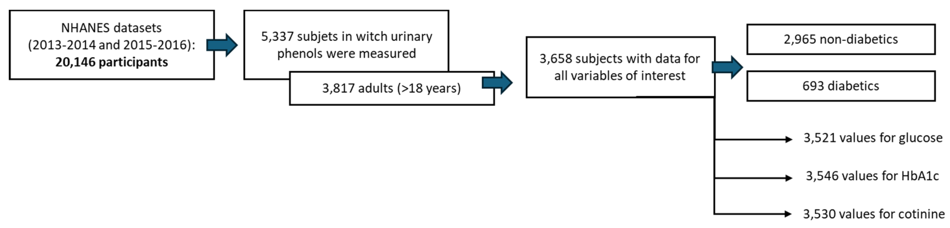
Figure 2.
Weighted quantile sum and quantile G-computation analysis of urinary Bisphenols in Diabetes. A) Weights derived from weighted quantile sum regression for the bisphenol mixture and Diabetes risk without confounder adjustment. B) Weights obtained from weighted quantile sum regression for the bisphenol mixture and Diabetes risk, adjusting the positive WQS regression model for confounders. C) Weights corresponding to the proportion of the positive or negative partial effect per chemical in the quantile g-computation model. D) Model fitting using Bootstrap. The graph of this model estimates the general effect of the mixture.
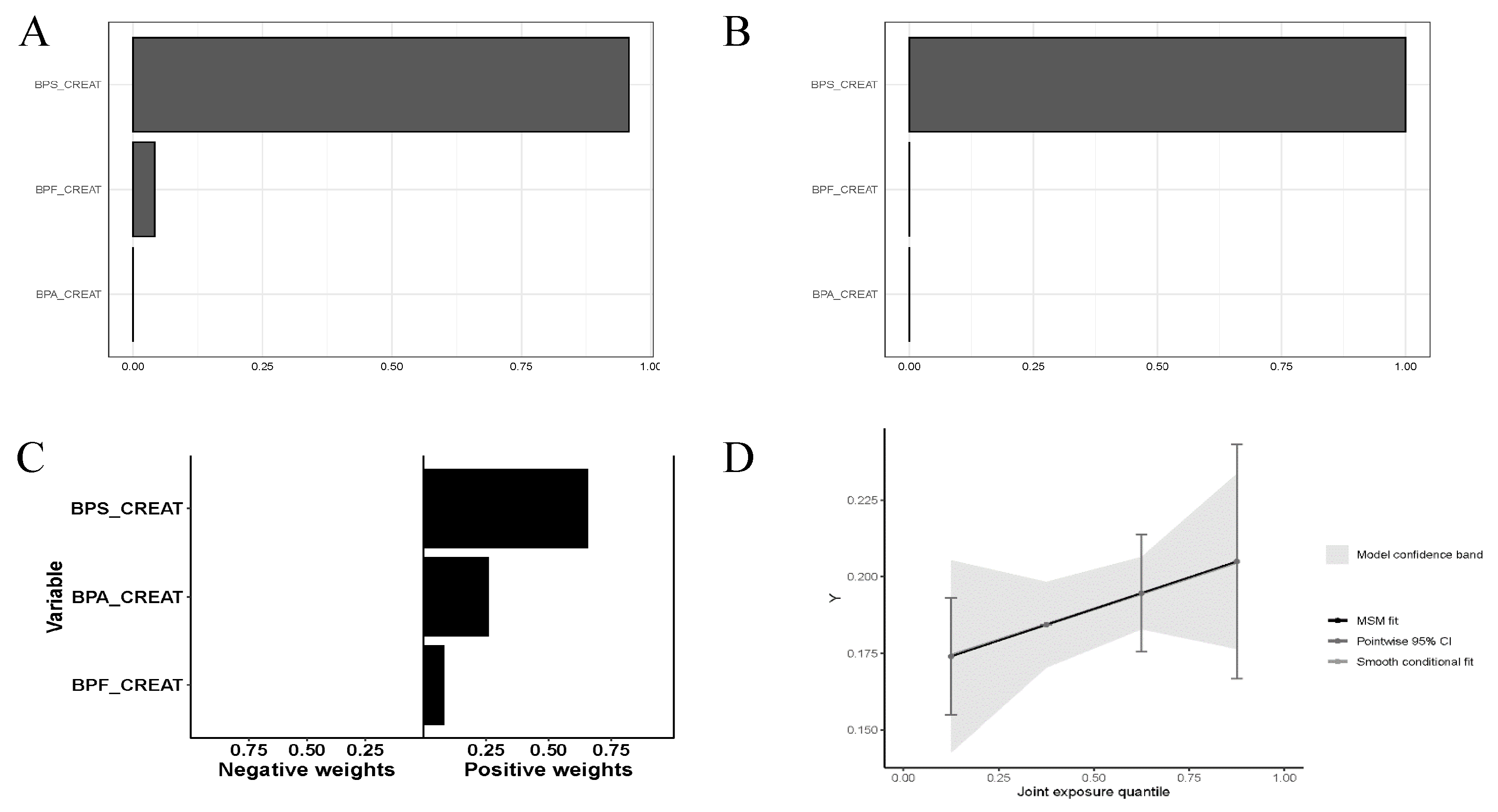
Figure 3.
Weighted quantile sum and quantile G-computation analysis of urinary Bisphenols and serum glucose. A) Weights derived from weighted quantile sum regression for the bisphenol mixture and serum glucose without confounder adjustment. B) Weights obtained from weighted quantile sum regression for the bisphenol mixture and serum glucose adjusting the positive WQS regression model for confounders. C) Weights corresponding to the proportion of the positive or negative partial effect per chemical in the quantile g-computation model. D) Model fitting using Bootstrap. The graph of this model estimates the general effect of the mixture.
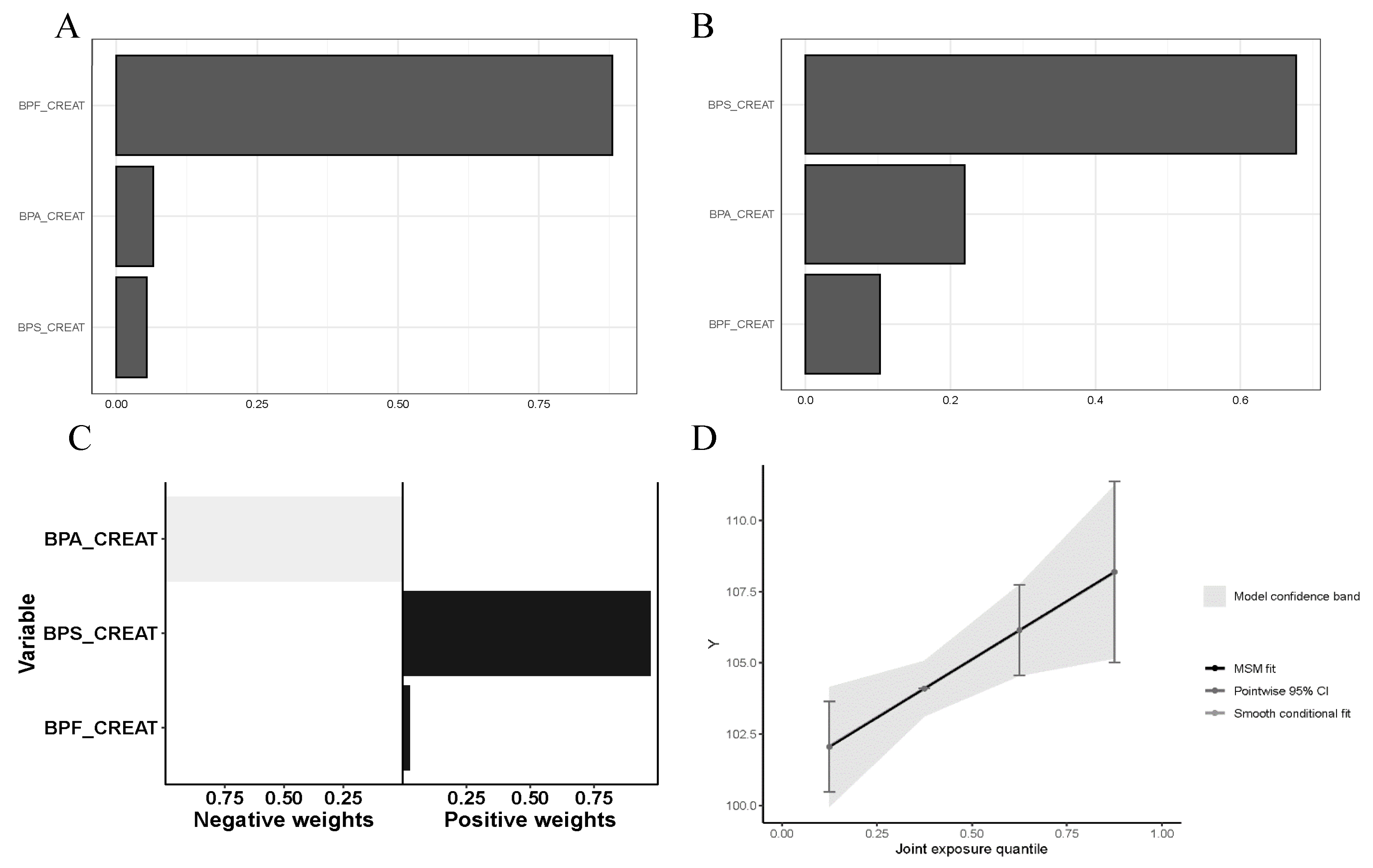
Figure 4.
Weighted quantile sum and quantile G-computation analysis of urinary Bisphenols and Hb1Ac. A) Weights derived from weighted quantile sum regression for the bisphenol mixture and Hb1Ac without confounder adjustment. B) Weights obtained from weighted quantile sum regression for the bisphenol mixture and Hb1Ac adjusting the positive WQS regression model for confounders. C) Weights corresponding to the proportion of the positive or negative partial effect per chemical in the quantile g-computation model. D) Model fitting using Bootstrap. The graph of this model estimates the general effect of the mixture.
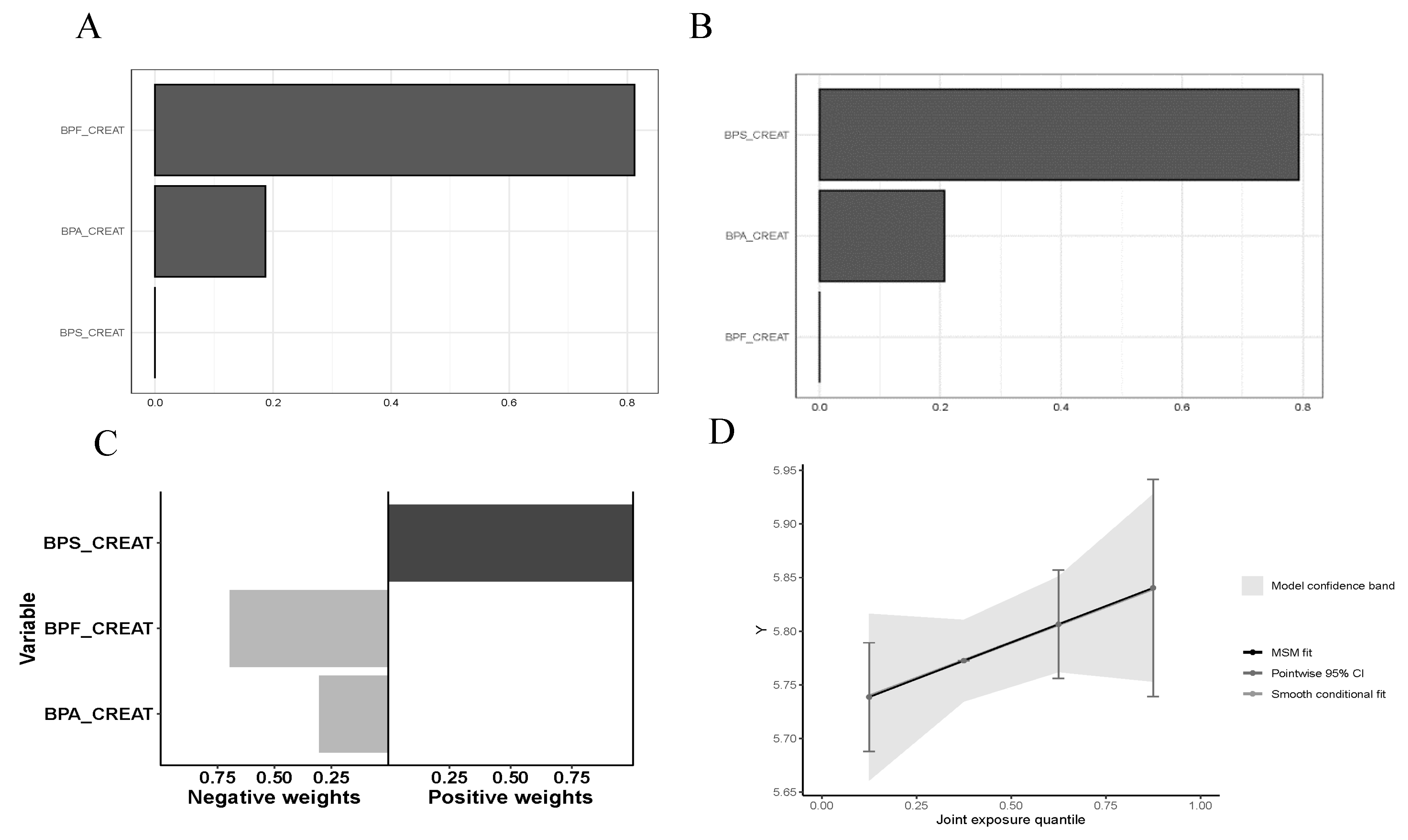

Table 1.
Descriptive examination of the urinary bisphenols mixture and relevant study covariates in relation to diabetes. Quantitative parameters are presented as Geometric Mean (95% Confidence Interval). Dichotomous variables are expressed as percentages. Statistical analysis of quantitative variables involved the use of the Mann-Whitney test while T-test or Fisher’s exact test was applied to dichotomous variables.
| Variable | Healthy (n=2965) | Diabetes (n=693) | p-value |
| Gender, men (%) | 1,389 (46.85) | 343 (49.50) | .112 |
| Age | 41.07 (40.43-41.71) | 57.08 (55.88-58.31) | .000 |
| BMI (kg/m2) | 27.8 (27.58-28.03) | 31.2 (30.69-31.72) | .000 |
| Mexican American | 434 (14.64) | 130 (18.76) | .000 |
| Other Hispanic | 317 (10.69) | 88 (12.70) | |
| Non-Hispanic White | 1125 (37.94) | 195 (28.14) | |
| Non-Hispanic Black | 640 (21.59) | 174 (25.11) | |
| Other Race - Including Multi-Racial | 449 (15.14) | 106 (15.30) | |
| Poverty-Income Ratio $ | 1.79 (0.83-3.81) | 1.53 (0.78-3.27) | .013 |
| Hypertension | 1043 (35.18) | 472 (68.11) | .000 |
| Dislipidemia | 993 (33.19) | 397 (57.29) | .000 |
| Smoking | 1266 (42.70) | 337 (48.63) | .003 |
| ΣBPs/Creat (µg/g) | 2.87 (2.78-2.97) | 3.2 (2.98-3.43) | .017 |
| ΣBP/Mol (nM) | 2.13 (2.03-2.23) | 2.21 (2.02-2.43) | .587 |
Abbreviations: BMI, Body Mass Index; BPs, the mixture of urinary bisphenols BPA, BPS and BPF; Creat, Creatinine. $ represents use of median (interquartile range).
Table 2.
ΣBPs/Creat (µg/g). Descriptive examination of covariates associated with urinary bisphenols, categorized by quartiles. The sample size (n) is specified for each subgroup. Geometric mean (95% Confidence Interval) is used to present quantitative parameters, while dichotomous variables are expressed as percentages. Statistical analysis for quantitative variables involved the application of Kruskal-Wallis followed by Dunn’s test, and Fisher’s exact test was employed for dichotomous variables.
| Variable | Q1 (n= 914) | Q2 (n= 915) | Q3 (n= 915) | Q4 (n= 914) | p-value |
| Diabetes (%) | 157 (17.2) | 169 (18.5) | 175 (19.1) | 192 (21.0) | .208 |
| Gender, men (%) | 533 (58.3) | 420 (45.9) | 386 (42.2) | 393 (43.0) | .000 |
| Age | 41.6 (40.5-42.8) | 44.6 (43.4-45.8)** | 44.1 (42.8-45.3)** | 44.61 (43.4-45.8)** | |
| BMI (kg/m2) | 28.3(27.9-28.7) | 28.2 (27.7-28.6) | 28.5 (28.1-28.9) | 28.7 (28.2-29.1) | |
| Mexican American | 139 (15.2) | 150 (16.4) | 144 (15.7) | 131 (14.3) | .000 |
| Other Hispanic | 86 (9.4) | 102 (11.1) | 110 (12.0) | 107 (11.7) | |
| Non-Hispanic White | 307 (33.6) | 325 (35.5) | 344 (37.6) | 344 (37.6) | |
| Non-Hispanic Black | 192 (21.0) | 204 (22.3) | 199 (21.7) | 219 (24.0) | |
| Other Race - Including Multi-Racial | 190 (20.8) | 134 (14.6) | 118 (12.9) | 113 (12.4) | |
| Poverty-Income Ratio $ | 2 (0.9-4.1) | 1.8 (0.8-3.6) | 1.7 (0.8-3.6) | 1.6 (0.8-3.4)** | |
| Hypertension | 338 (37.0) | 396 (43.3) | 378 (41.3) | 403 (44.1) | .010 |
| Dislipidemia | 327 (35.8) | 352 (38.5) | 341 (37.3) | 370 (40.5) | .204 |
| Smoking | 360 (239.4) | 370 (40.4) | 419 (45.8) | 454 (49.7) | .000 |
Abbreviations: BMI, Body Mass Index. $ represents use of median (interquartile range). ** is equivalent to a p-value ≤ 0.01.
Table 3.
ΣBPs/Mol (nM). Descriptive examination of covariates associated with urinary bisphenols, categorized by quartiles. The sample size (n) is specified for each subgroup. Geometric mean (95% Confidence Interval) is used to present quantitative parameters, while dichotomous variables are expressed as percentages. Statistical analysis for quantitative variables involved the application of Kruskal-Wallis followed by Dunn’s test, and Fisher’s exact test was employed for dichotomous variables.
| Variable | Q1 (n= 916) | Q2 (n= 915) | Q3 (n= 912) | Q4 (n= 915) | p-value |
| Diabetes (%) | 158 (17.2) | 195 (21.3) | 174 (19.1) | 166 (18.1) | .142 |
| Gender, men (%) | 416 (45.4) | 444 (48.5) | 450 (49.3) | 422 (46.1) | .274 |
| Age | 45.4 (44.2-46.7) | 44.8 (43.6-46) | 42.4 (41.2-43.6)** | 42.4 (41.2-43.6)*** | |
| BMI (kg/m2) | 27.1 (26.7-27.5) | 28.2 (27.8-28.6)**** | 29 (28.6-29.5)**** | 29.3 (28.9-29.8)**** | |
| Mexican American | 122 (13.3) | 131 (14.3) | 159 (17.4) | 152 (16.6) | .000 |
| Other Hispanic | 69 (7.5) | 110 (12.0) | 119 (13.0) | 107 (11.7) | |
| Non-Hispanic White | 424 (46.3) | 342 (37.4) | 294 (32.2) | 260 (28.4) | |
| Non-Hispanic Black | 131 (14.3) | 183 (20.0) | 213 (23.4) | 287 (31.4) | |
| Other Race - Including Multi-Racial | 170 (18.6) | 149 (16.3) | 127 (13.9) | 109 (11.9) | |
| Poverty-Income Ratio $ | 2.4 (1 – 4.5) | 1.8 (0.9-3.5)**** | 1.5 (0.7-3.2)**** | 1.5 (0.7-3.3)**** | |
| Hypertension | 364 (39.7) | 395 (43.2) | 362 (39.7) | 394 (43.1) | .225 |
| Dislipidemia | 353 (38.2) | 366 (40.0) | 347 (38.0) | 324 (35.4) | .234 |
| Smoking | 372 (40.6) | 417 (45.6) | 409 (44.8) | 405 (44.3) | .142 |
Abbreviations: BMI, Body Mass Index. $ represents use of median (interquartile range). ** is equivalent to a p-value ≤ 0.01; *** is equivalent to a p-value ≤ 0.001; **** is equivalent to a p-value ≤ 0.0001.
Table 4.
Pearson correlation coefficient analysis of quantitative variables.
| ΣBPs/Creat | ΣBPs / Mol | Glucose | HbA1c | Cholesterol | Cotinine | |
| ΣBPs / creat | 1 | ** | - | * | - | ** |
| ΣBPs / Mol | .391** | 1 | - | * | - | ** |
| Glucose | .033 | .031 | 1 | ** | - | * |
| HbA1c | .035* | 0.36* | .757** | 1 | - | * |
| Cholesterol | .009 | -.017 | .007 | .029 | 1 | - |
| Cotinine | .085** | .078** | -.040* | -.033* | -.015 | 1 |
Abbreviations: BPs, Bisphenols (BPA+BPF+BPS); Hb1Ac, glycated haemoglobin or glycosylated haemoglobin. * is equivalent to a p-value ≤ 0.05; ** is equivalent to a p-value ≤ 0.01. Quantitative values for the variables of interest were available for 3,530 patients for cotinine, 3,521 for glucose, and 3,546 for HbA1c.
Table 5.
Association between Urinary Bisphenol Mix and Diabetes (Odds Ratio) – Binomial Logistic Regression Analyses. Analysis performed individually (1), adjusted for age, gender, and BMI (2), and further adjusted for (2) + race/ethnicity, poverty-income ratio, hypertension, dyslipidemia, and smoking (3). Log-transformed urinary concentrations of bisphenol metabolites for normalized distributions.
| BP mixture | Covariates | OR (95 % CI) | p-value |
| ΣBPs / creat | 1 | 1.132 (1.038-1.235) | .005 |
| 2 | 1.102 (1.003-1.211) | .043 | |
| 3 | 1.103 (1.002-1.214) | .045 | |
| ΣBPs / Mol | 1 | 1.024 (0.960-1.092) | .468 |
| 2 | 1.024 (0.955-1.097) | .509 | |
| 3 | 0.989 (0.920-1.064) | .773 |
Abbreviations: BPs, Bisphenols (BPA+BPF+BPS); OR, Odds Ratio; CI, Confidence Interval.
Table 6.
Multinomial Logistic Regression of Diabetes and Bisphenols Quartile. Quartile 1 serves as the reference group in the statistical model. Binomial logistic regression analyses were conducted in three ways Analysis performed individually (1), adjusted for age, gender, and BMI (2), and further adjusted for (2) + race/ethnicity, poverty-income ratio, hypertension, dyslipidemia, and smoking (3.
| Q1 | Q2 | Q3 | Q4 | |
| Variable | Ref. | OR (95% CI) | OR (95%CI) | OR (95%CI) |
| 1Diabetes (1) | Ref. | 1.09 (0.86-1.39) | 1.14 (0.90-1.45) | 1.28 (1.01-1.62)* |
| 1Diabetes (2) | Ref. | 1.01 (0.78-1.30) | 1.05 (0.81-1.36) | 1.16 (0.90-1.50) |
| 1Diabetes (3) | Ref. | 1.03 (0.80-1.34) | 1.10 (0.85-1.43) | 1.21 (0.93-1.56) |
| 2Diabetes (1) | Ref. | 1.30 (1.03-1.64)* | 1.13 (0.89-1.44) | 1.06 (0.84-1.35) |
| 2Diabetes (2) | Ref. | 1.27 (0.99-1.62) | 1.12 (0.87-1.45) | 1.04 (0.80-1.35) |
| 2Diabetes (3) | Ref. | 1.14 (0.89-1.48) | 0.98 (0.76-1.28) | 0.89 (0.68-1.17) |
OR, Odds Ratio; CI, Confidence Interval. 1 ΣBPs / creat. 2 ΣBPs / Mol. * is equivalent to a p-value ≤ 0.05.
Disclaimer/Publisher’s Note: The statements, opinions and data contained in all publications are solely those of the individual author(s) and contributor(s) and not of MDPI and/or the editor(s). MDPI and/or the editor(s) disclaim responsibility for any injury to people or property resulting from any ideas, methods, instructions or products referred to in the content. |
© 2025 by the authors. Licensee MDPI, Basel, Switzerland. This article is an open access article distributed under the terms and conditions of the Creative Commons Attribution (CC BY) license (http://creativecommons.org/licenses/by/4.0/).
Copyright: This open access article is published under a Creative Commons CC BY 4.0 license, which permit the free download, distribution, and reuse, provided that the author and preprint are cited in any reuse.


