
Submitted:
22 May 2025
Posted:
23 May 2025
You are already at the latest version
Abstract
Time-domain (TD) diffuse reflectance can be quantified using photon diffusion theory (DT) to non-invasively obtain optical transport coefficients of biological media, which in turn provide markers of tissue physiology. We use an optimized, N-layer numerical DT solver in cylindrical geometry to recover optical coefficients of bi-layered media using time-resolved reflectance generated by Monte Carlo (MC) simulations. Optical coefficients for each layer of 384 bilayered tissue models were obtained from literature to model human head or limb tissue, at three near-infrared wavelengths. We fit MC data using a layered DT model to reconstruct transport coefficients of both layers simultaneously. We could retrieve bottom-layer absorption with errors less than 0.02 cm−1 while top-layer scattering was recovered to 3 cm−1 of input values. Reconstructions of the bottom-layer scattering had a mean error greater than 50%. Total hemoglobin concentration and fractional oxygen saturation were reconstructed in both layers and were within 10 μM and 5%, respectively, for the bottom layer. Recovered values of transport coefficients were significantly improved with the layered DT compared to the more widely used semi-infinite DT. Findings suggest that incorporating layered models in fitting TD reflectance could enhance its value in applications.
Keywords:
Time resolved diffuse reflectance
; Time domain transport
; NIRS
; Spectroscopy
; Diffusion Approximation
1. Introduction
Time domain diffuse optical spectroscopy (TD-DOS) is a quantitative, non-invasive technique that has been widely explored across several biomedical applications [1,2,3,4,5]. The quantitative nature of this technique relies on recovering the wavelength-dependent transport coefficients –the absorption coefficient and the reduced scattering to optically characterize the medium from which measurements are obtained. In TD-DOS, the measured temporal attenuation and broadening of an input source (which experimentally is usually a laser having pulse durations of 10-100 ps) is mathematically modeled using theoretical or numerical methods to recover the optical coefficients and [6,7,8,9,10]. In human tissues, accurate recovery of at multiple wavelengths allows for reconstructions of component chromophore concentrations such as hemoglobin, water, and/or lipids, while is influenced by tissue microstructure [6,9,11,12,13,14]. These chromophore concentrations are used to estimate tissue vascular oxygen saturation, total blood volume, hydration, and/or cellular density in vivo [15,16,17].
Theoretical models are critical for recovering optical transport coefficients from measurements, as they provide the quantitative platforms to model light transport in turbid media. A commonly used theoretical approach to quantify TD-DOS measurements is diffusion theory (DT)[18,19,20,21,22]. DT-based approaches typically consider the tissue medium as optically-homogeneous and semi-infinite in extent across in various applications, including tracking and monitoring cerebral oxygenation and cancer development in clinical settings [3,8,19,23,24]. Though modeling biological tissues as a semi-infinite homogeneous medium allows for quantitative analysis, it is inherently insensitive to any inhomogeneities of the medium, which has been shown to lead to large errors in recovering physiological parameters [6,7,9,25,26,27].
Representing tissue as a bilayered medium would be more realistic than as a semi-infinite medium –e.g., a human head can be better modeled as having a top layer (representing scalp and skull) and a bottom layer (for the cerebral spinal fluid, gray and white matter) and limb tissues can be modeled as a layer of muscle buried under a upper-layer of fat and skin [6,28]. The use of layered models in DT would permit reconstruction of optical coefficients for each layer, independently, from the measured TD reflectance [11,17,29]. Bilayered models can thus naturally detect transport coefficients of deeper layers better, and could also be used to suppress cross-talk from superficial layers [21,30,31]. Such depth-dependent reconstructions would enhance the accuracy of cerebral and muscular hemodynamic assessments [29,30,32,33,34,35].
Analytical solutions of TD reflectance using DT in bilayered media have been reported previously [18,36,37,38,39]. However, they are not commonly used as the implementation of these solutions require computing complex analytical expressions that often include hyperbolic functions, leading to numerical instabilities because of finite machine-precision. Thus, these solvers have high computational complexity and costs [7,35,40,41,42,43]. Recently, we have developed an easy-to-use, open-source library - lightPropagation.jl - that is numerically stable and highly optimized (with a single calculation for a forward solution taking less than ms on standard laptop computers) for computing time domain reflectance in multilayered tissue models via DT [44].
Here, we seek to establish the accuracy and precision of using lightPropagation.jl for inverse reconstruction of optical coefficients using time-domain reflectance acquired from using Monte Carlo (MC) simulated of time-resolved reflectance in bilayered tissue models. We assess the performance of the inverse model in recovering the absorption and reduced scattering coefficients. To ensure appropriate relevance to biomedical applications, we selected optical properties for tissue models simulated to match values reported in literature [28]. We use wavelength-dependent reconstructions to derive functional biological markers of fractional oxygen saturation () and hemoglobin concentrations for each tissue layer and quantify the errors associated with reconstructions to establish limits for accuracy and precision of recovered optical coefficients and functional endpoints.
2. Materials and Methods
2.1. Bi-Layered Tissue Models
Two types of tissue models, representing head and limb muscle tissue were used to generate TD reflectance using MC simulations and are depicted by Figure 1(a). Both tissue models were represented as cylinders with large radius (set to 100 cm), had upper layer thickness of 1 cm, and had semi-infinite bottom layer (thickness of 100 cm) to compute MC and DT solutions. Input values of the absorption coefficient for each layer in each tissue model was determined by solely by two chromophores - oxygenated ([HbO]) and deoxygenated hemoglobin ([dHb]) [45]. Table 1 lists values for inputs used to generate optical coefficients in each layer, for each tissue model.
Eq.(1) was used to determine for each layer by specifying values for and and using molar extinction coefficients and from literature [28,46]. The reduced scattering coefficients () for the top and bottom layer were calculated using Eq.(2) using literature values for A and b, for each layer and tissue type [12,28].
64 different models were generated at three commonly used near infrared wavelengths (690, 760, and 850 nm) to span the isosbestic points of hemoglobin [6,14,20]. The full dataset consisted of bilayered tissue models, on which we conducted the analysis. Ranges for optical coefficients at each of the three wavelengths used, for each layer, are listed in Table A1, Table A2 and Table A3 for 690 nm, 760 nm and 850 nm, respectively.
2.2. Monte Carlo Simulation of Reflectance Signals
A previously used Monte Carlo code for photon transport was used to simulate time-resolved reflectance from each of the 384 tissue models [47,48]. MC simulations for all models were computed with photons. For each simulation, the input source was a pencil beam (representing a delta-function) incident at the origin of the tissue model and the TD diffuse reflectance was recorded between 1cm to 3 cm in intervals of cm with timing relative to the input delta-function source. Reflectance data was stored between ns with temporal resolution of ns simulations were run on a high-performance computing cluster (with each node of the cluster hosting Intel Xeon Gold processors). Each MC simulation required about 15 hours to execute and simulations were run in parallel (on separate compute nodes) to increase output efficiency. For analysis, each simulated time-resolved reflectance was smoothed (using a moving-window of span 5 or a temporal window of 0.05 ns), normalized (peak intensity ), truncated (by retaining values greater than of peak intensity of the rising edge to eliminate early arriving photons and lesser than than of the tail to limit statistical noise), and lastly log-transformed to obtain . Although we simulated reflectance data between 1-3 cm, we only use reflectance at three specific source detector separations (SDS) of 1.5, 2 & 2.5 cm because the noise in MC simulations at SDS of 3 cm was too high for use here.
2.3. Forward-Modeling of Diffuse Reflectance Signal
The numerical DT solver lightPropagation.jl was used to obtain the TD-reflectance (the temporal point spread function or TPSF), for any given bilayered cylindrical tissue model [27]. The SDS and was set to match those from the MC simulations, the refractive index of each layer was fixed to be which is consistent for biological tissues from previous work [49] and the top layer thickness was set to 1 cm. To compute the reflectance signal, for each tissue model required inputs for the four transport coefficients, , , and . The computed signal was was then truncated, normalized and log-transformed following the same protocol used for processing the MC reflectance signal, to obtain .
Figure 1(b) shows representative data for TD-reflectance simulated (in symbols) and predicted from DT (solid lines) at three different wavelengths (colors) for a muscle tissue model. The values of optical absorption and scattering were calculated at each wavelength using Eq.(1) and Eq.(2) where was M for the top layer and M and for bottom layer, with both layers having of 50%.
2.4. Inverse Fitting of Reflectance
Inverse modeling sought to recover the four optical transport coefficients (the absorption and scattering for each layer) by fitting each time-resolved reflectance , at each SDS, for each of the 384 tissue models. Fits were obtained iteratively using a Levenberg-Marquardt non-linear optimizer (LVM) (LsqFit package in Julia version 1.9.1) to compute a set of inputs to compute that best matched the input . For DT calculations, the top layer thickness was assumed to be known (kept fixed for all analysis here at 1 cm), the refractive indices of both layers were held fixed at and the SDS was set to match . During optimization the optical coefficients were constrained to be bounded between for absorption and between for scattering.
A normalized mean absolute error () value was computed to evaluate goodness of fits between and using equation 3
Here, represents the average of the absolute value of the reflectance signal, and . N represents the total number of time bins in and across the entire data-set, due to data truncation of that was noted above.
For each simulated reflectance , inverse fitting was repeated until . If was higher than this after 25 attempts the solution with lowest was used as the fit. In Figure 1(b) inverse fits are shown by dashed lines and had for 690 nm (indigo), 760 nm (orange) and 850 nm (red) models, respectively.
Lastly, we also used the semi-infinite DT approximation to fit using lightPropagation.jl [27]. The forward fitting used in lightPropagation.jl replicates the expression for semi-infinite DA reflectance in Ref.[37]. Inverse fitting for the semi-infinite model mirrored the bilayered approach, and used the optimizer algorithm to extract two coefficients and to the same goodness-of-fit threshold as used in the bi-layer reconstructions () and used the same search ranges for each optical coefficient (; ).
2.5. Retrieval of Functional Endpoints
As most real-world applications of TD-DOS involve extracting tissue physiological parameters from optical coefficients we emulated that process to the reconstructed absorption coefficients at multiple wavelengths to obtain the functional parameters of and using 4
Here, values of and were estimated using the same optimizer (as used for TD-reconstructions) to ensure only non-negative values of and were allowed as solutions by the optimizer. This eliminated any solutions with negative values for concentrations and thus remain physiologically meaningful. The chromophore concentrations were used to compute (as +) and fraction (as ) which were each then compared to input values used for each model (shown in Table 1). This process was repeated for each SDS.
3. Results
The inverse fitting protocol was employed to recover optical coefficients from each of the 384 MC models at three SDS. Reconstructions for the absorption (, ) and reduced scattering coefficients (, ) at 760 nm are shown in Figure 2. The mean goodness of fits at cm and 2 cm had , across all models, with head reconstruction performing marginally better (average (head) was lesser than (muscle)). However, for SDS of cm, increased to which we hypothesize was due to an increase in statistical noise in the MC simulations at longer SDS. Each iteration for convergence took approximately on average and most fits needed iterations to meet the required convergence threshold. In Figure 2 each marker corresponds to some fixed value for the optical coefficient being plotted, while the other three coefficients were varied. For instance, each marker in Figure 2(a) is from 16 different tissue models that shared the same value, while error bars are the standard error across all those 16 reconstructed values of as , and were permuted.
Figure 2(d) clearly show that the largest reconstruction errors were seen bottom layer scattering with reconstruction errors, generally for all SDS. The difficulty of layered DT in reconstructing deep-layer scattering estimation observed here has been reported previously [18,50,51]. Recovery of was inconsistent and showed significant errors for some of the tissue models tested but the mean reconstruction error was lower than at SDS cm and 2 cm, with good agreement in many cases, as noted in Figure 2(a) by the overlapping markers. Larger errors in reconstructed values for were noted at SDS of 2.5 cm growing to nearly . Recovery of and were the highly accurate with errors , respectively, for all SDS tested. These trends preserved at the other two wavelengths (Supplementary Figure A1 for 690 nm and Figure A2 for 850 nm)
The impact of reconstruction errors on derived physiological parameters was next investigated by computing the reconstructed concentrations of () and (), as illustrated in Figure 3. Reconstructed absorption coefficients at 690 nm, 760 nm, and 850 nm were used to derive the hemoglobin concentrations. Due to the sparse and non-uniform distribution of hemoglobin concentrations used in simulated tissue models, the x-axis are scaled to reflect the actual concentration values and thus the values from bar heights need to interpreted in conjunction with their x-axis locations, to assess performance of reconstructions.
Results in Figure 3(a) and Figure 3(b), demonstrate that top-layer hemoglobin retrieval was less accurate than reconstructions in the bottom layer. Most of the reconstructed values in the upper layer either overestimated (for smaller values of ) or underestimated (for larger values of ). For instance, the reconstructed value for was M when its true value was M for muscle (the third bar in Figure 3(a)). However, the spread (standard error) remained within M across all models which is sufficient for clinical use [52]. The reconstructions for bottom-layer concentrations were accurate overall, with reconstructed values for both and being well within the computed standard error (Figure 3(c) and Figure 3(d)). This trend was true at all SDS used, but data at larger SDS were associated with a larger spread in reconstructed values.
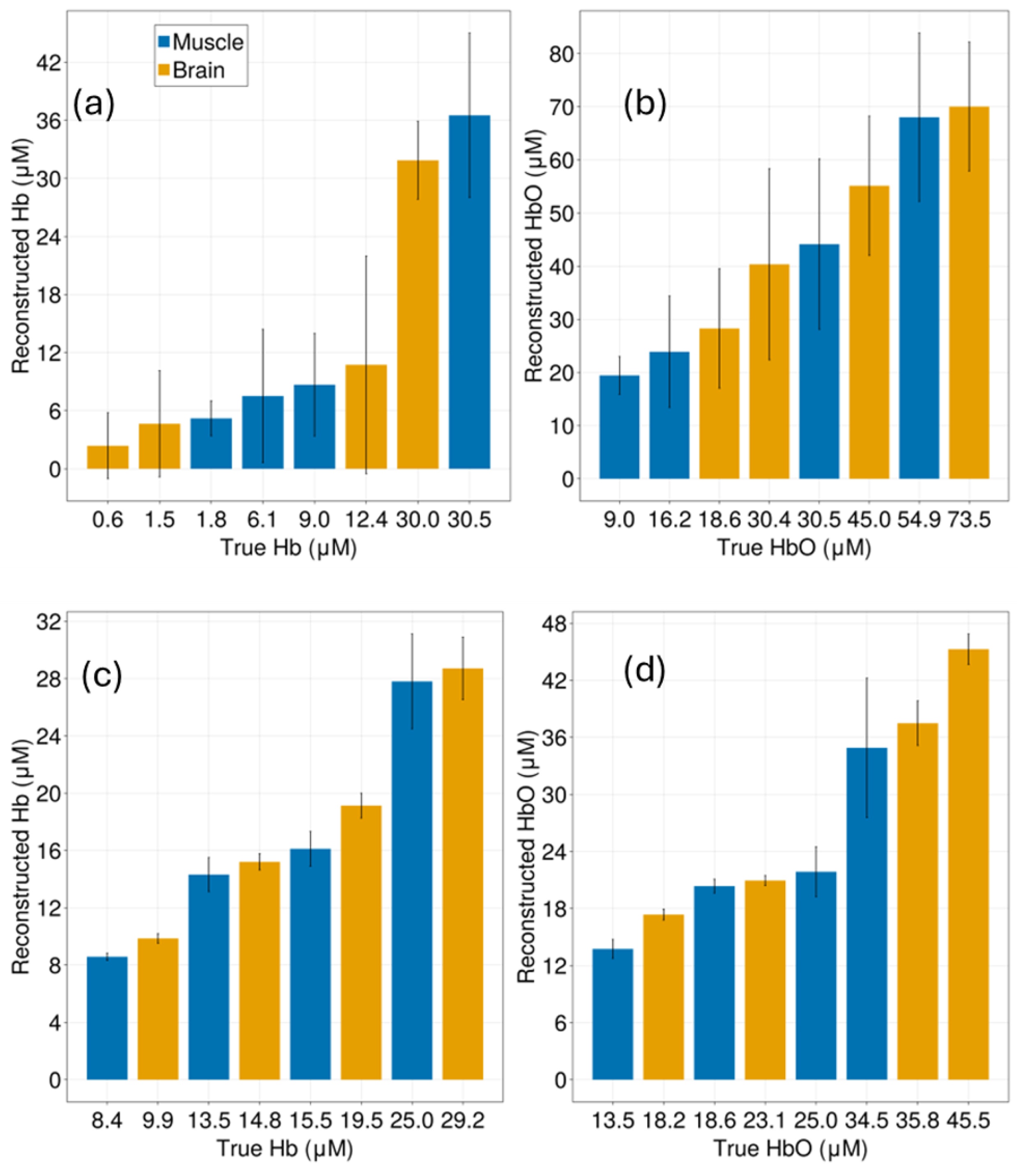
Functionally, the most common biomarkers sought by real-world applications using TD-DOS include the total hemoglobin concentration and fractional oxygen saturation which are computed using wavelength-dependent optical transport coefficients. Figure 4 shows the true (input) values used for and total hemoglobin concentration values for the top and bottom layers vs. those derived from the inverse DT. As expected and seen in the figures, errors in hemoglobin concentrations of the top layer directly affect the accuracy of the derived physiological markers of and , leading to significant deviations from their true values.
These appear as incorrect median reconstructed values as well as higher standard error all SDS. However, both precision and accuracy of reconstructed values for the bottom layer (Figure 4(c) and Figure 4(d)) were excellent with the reconstructed median values of both and matching the expected physiological ranges to better than 3% across all SDS. One exception to this was seen for muscle models where M and (for the bottom layer) that exhibited large standard error in derived values (the median value was in agreement to the true value to within 3% again) . These same tissue models shown in Figure 3 also had large standard errors in reconstructed and [] concentrations.
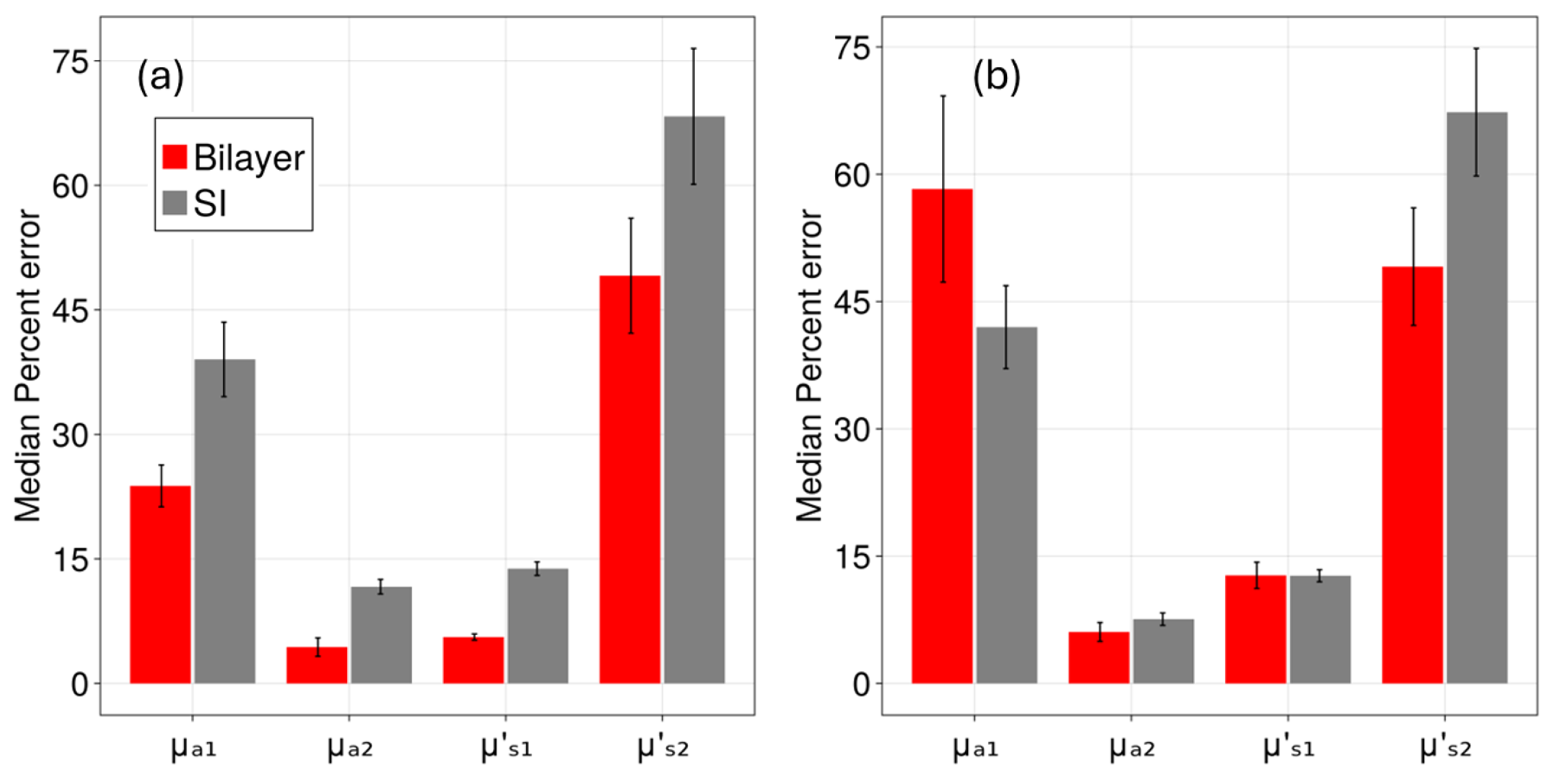
As a final point of analysis, we reconstructed optical coefficients from the bilayered using the semi-infinite DT expression for TD reflectance. Since the SI model reconstructed optical coefficients for a homogeneous model (hence only recovers two optical coefficients), we compared the recovered absorption coefficient to both and and repeated that for the reduced scattering as well. Figure 5, shows the median percent error (bars) along with the standard error (error bars) for all MC models (head and tissue) simulated at 15 mm SDS. It is clear that even with the difficulties in reconstruction of four optical coefficients using bi-layer DT models, the retrieved layer specific transport coefficients were always more accurate than those estimated by the semi-infinite model with a notable exception for retrieval of . This is also true for SDS cm but at SDS cm, the reconstruction of was significantly affected (Figure A5)
4. Discussion
We verified the accuracy of a recently reported, open-source, numerical solver of DT in cylindrical coordinates, lightpropagation.jl, to function as an inverse solver in bilayer tissue models using TD reflectance simulated at multiple SDS. 384 bilayered models were simulated using MC for a range of tissue optical properties that have been reported for head and muscle tissues. The goodness of fit was established by computing the Normalized Mean Absolute Error (), which on average was (across all models) lower than 0.01 at SDS and 2 cm while at SDS of cm. A change of 0.01 in in goodness of fit significantly impacted accuracy of reconstructions of the top layer absorption as seen in Figure 2(a) (and Figure A1(a) Figure A2(a)). Thus could potentially signal a measure of confidence in the retrieved value of optical coefficients for each fitted reflectance and could also serve as a measure of signal quality in experimental use.
A threshold of in inverse fits of the reflectance was sufficient for reconstruction of top layer scattering () and the bottom layer absorption () with mean errors of lesser than 5% (for ) and lower than 3% (for ), across all SDS tested and as shown in Figure 2(b)-(c) Figure A1(b)-(c) and Figure A2(b)-(c). However, the scattering of the bottom layer () could not be reconstructed accurately and showed average error of more than 60% across all SDS, indicating layered DT is largely unperturbed by changes in deep-layer scattering, as reported before [7,18,39,50,51]. Although recovery of top layer absorption was achieved, it was inconsistent, with mean errors for all 384 models at SDS and 2 cm that increased to more than 50 % for SDS of 2.5 cm, which indicates that the reconstruction upper layer absorption was highly sensitive to SNR.
The input coefficients for each tissue model simulated here were obtained by assuming only two chromophores ( and ) were present in each layer, the values are shown in Table 1. In the inverse sense, these chromophore concentrations had to be obtained from reconstructed absorption coefficients, for each layer, at each wavelength. Thus, as expected, errors in recovery of impacted the estimation of oxygenated and deoxygenated hemoglobin concentrations for the upper layer, with mean error being higher than M but lower than M for SDS cm (Figure 3(a)-(b) and Figure A3(a)-(b)). The upper bound on of top-layer concentration errors grew to more than M for both chromophore concentrations at SDS of cm (Figure A4(a)-(b)). The bottom-layer reconstructions demonstrated good agreement with ground truth values (to better than M at all SDS) while also having low inter-model variance.
Accurate recovery of individual chromophore concentrations is important, as clinically relevant parameters such as oxygen saturation () and total hemoglobin concentration () are derived from the combined contributions of and as markers of tissue health and metabolic demand. Errors in reconstruction of the top layer chromophore concentrations thus impacted retrieval of top layer (error > 5% for all SDS). The top layer values were retrieved with mean errors greater than 15% for shorter SDS (1.5 and 2 cm), which increased to more than for larger SDS (Figure 4(a)-(b)). Again, this is consistent with the idea that the diffuse reflectance collected at larger SDS would be most insensitive to upper layer optical coefficients.
These results highlight that bilayered DT has reduced sensitivity to the top layer absorption and reconstruction of is sensitive to signal quality. However, recovery of bottom layer endpoints was accurate with and being estimated to better than 3% across all SDS. This result is particularly encouraging since it signifies that real-world applications could enhance the quantitative sensitivity of functional properties recovered from deeper tissue layers, while being immune to changes in superficial layers, by using improved analytical models for reconstruction of TD reflectance [11,53,54].
A practical consideration that remained significant was the computational cost involved with reconstructions using the bilayer inverse model. The inverse fits converged in under 100 milliseconds using the analytical DT expression for a SI model, while for bilayer reconstructions inverse fits were approximately three orders of magnitude slower (taking about 150 s for each model). All inverse calculations were run on nodes of a high-performance computing cluster (with each node having an Intel Xeon Gold processor). For the 384 models analyzed at 3 SDS, the total computation time was almost 40 CPU-hours. This disparity presents a significant bottleneck for real-time or high-throughput analysis and motivates the development of computationally efficient strategies or machine-learning based models for acceleration.
Ultimately, the computational costs were recovered by the layered model as it consistently outperformed the semi-infinite model in terms of accuracy to recover and even at large SDS (Figure 5 and Figure A5). On average the bilayered modeling performed about 10 - 15% better than SI model, across optical coefficients (except ) at SDS cm. It is interesting to note that bilayered DT models could extract accurately, even for shorter SDS could prove to be practically useful, as shorter SDS channels usually have better SNR.
5. Conclusions
We showed that using multi-layer DT for analysis of TD reflectance in bilayered media allowed for quantitative reconstruction of optical absorption of both layers with errors well within requisite thresholds for clinical utility. 64 different head and limb models at three commonly used near infrared wavelengths were used to simulate a total of 384 MC reflectance signals used for our analysis. For the top layer, absorption coefficient () was reconstructed with mean errors at SDS cm (rising to at 2.5 cm), while reduced scattering coefficient () showed high accuracy ( across all SDS). Bottom layer absorption, on the other hand was retrieved exceptionally well ( error) while bottom layer scattering could not be well estimated. These translated to errors in biomarkers with top-layer and values having larger errors relative to the bottom-layer, highlighting the utility of layered DT to assess depth-resolved tissue physiology. Layered DT always outperformed semi-infinite DT, across all retrieved optical coefficients but had significantly higher computational costs. Future work will investigate approaches to reduce computational time for optimization, for e.g., by using SI DT to bootstrap the optimization, or to exclude reconstructions. Approaches that reduce dimensionality of the inverse problem could potentially accelerate reconstructions without sacrificing accuracy.
Author Contributions
Conceptualization, S.R. and K.V; methodology, S.R. and K.V; software, S.R.; validation, S.R. and K.V.; investigation, S.R.; writing—original draft preparation, S.R.; writing—review and editing, S.R. and K.V.; visualization, S.R.; supervision, K.V.; All authors have read and agreed to the published version of the manuscript.
Funding
This research received no external funding.
Institutional Review Board Statement
Not applicable.
Data Availability Statement
LightPropagation.jl is a registered Julia package that can be installed on a Julia version > 1.5. The MC simulations and inverse fitting codes are available on request.
Acknowledgments
This work builds upon the computational advancements of Dr. Michael Helton (University of Michigan), developer of LightPropagation.jl – a Julia-based toolbox for solving time-resolved photon migration in turbid media . We also thank Dr. Jens Müller for facilitating high-performance simulations on the Miami Redhawk cluster.
Conflicts of Interest
The authors declare no conflicts of interest.
Abbreviations
The following abbreviations are used in this manuscript:
| SI | Semi Infinite |
| DT | Diffusion Theory |
| MC | Monte Carlo |
| TPSF | Temporal Point Spread Function |
| THb | Total Hemoglobin Concentration |
| Fractional Oxygen Saturation | |
| SDS | Source Detector Separation |
| SNR | Signal to Noise Ratio |
Appendix A. Computed Optical Transport Coefficients
Here we report the computed optical coefficients using the ranges for and described in Table 1.

Table A1.
The selected target tissue properties. The values below were calculated for nm. The value reported for each optical property is the mean of the coefficients (4 for absorption for each layer and 2 for scattering for ech layer) along with the range covering all the computed values. The coefficient values used for our analysis for each model, however were not evenly spread within this range.
| Tissue Model | Layer | ||
|---|---|---|---|
| Head | Top (scalp,skull) | ||
| Bottom (Brain) | |||
| Muscle | Top (skin,fat) | ||
| Bottom (Muscle) |
Table A2.
The values below were calculated for nm.
| Tissue Model | Layer | ||
|---|---|---|---|
| Head | Top (scalp,skull) | ||
| Bottom (Brain) | |||
| Muscle | Top (skin,fat) | ||
| Bottom (Muscle) |
Table A3.
The values below were calculated for nm.
| Tissue Model | Layer | ||
|---|---|---|---|
| Head | Top (scalp,skull) | ||
| Bottom (Brain) | |||
| Muscle | Top (skin,fat) | ||
| Bottom (Muscle) |
Appendix B. Reconstruction of Optical Coefficients
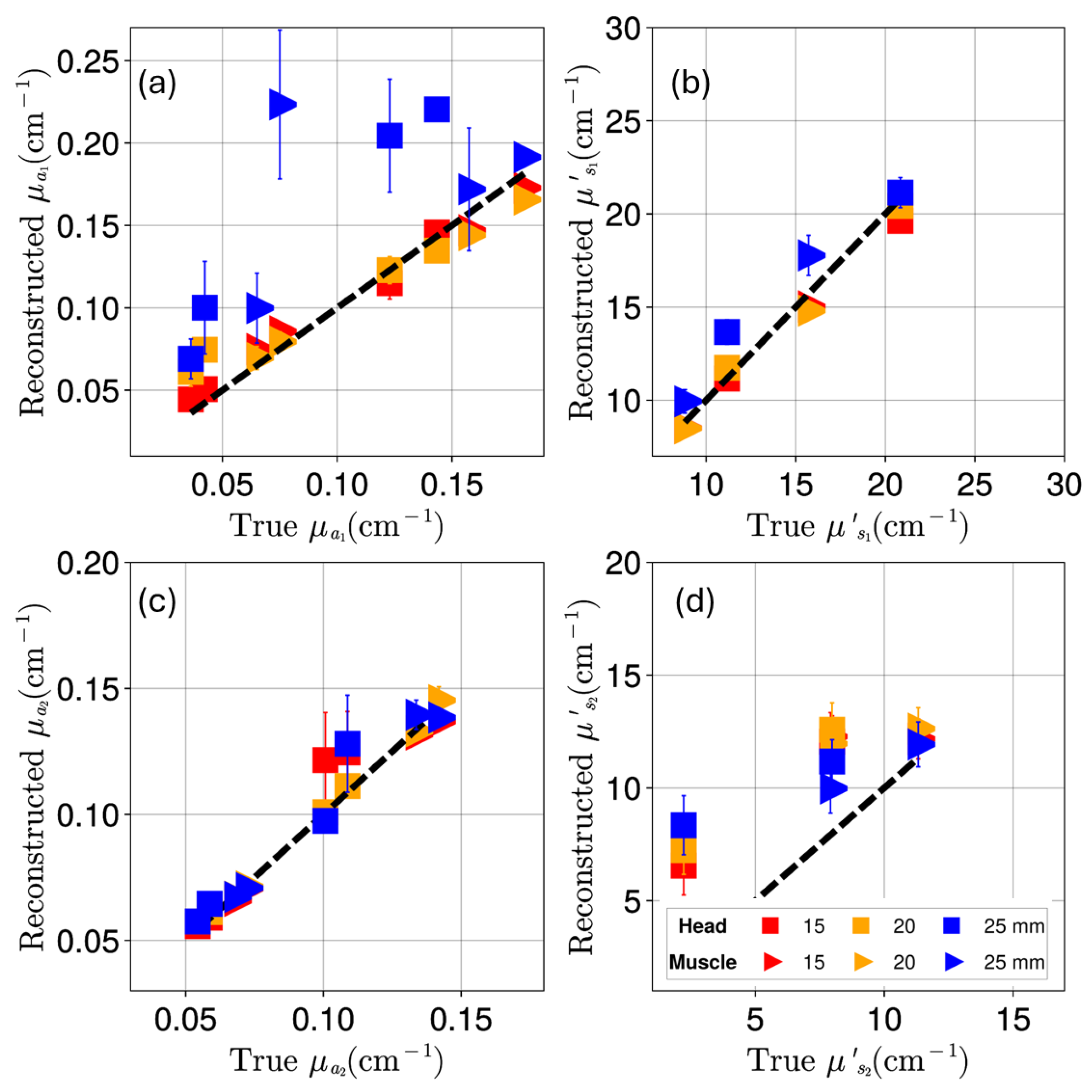
The optical coefficients recovered across all source-detector separations exhibited consistent recovery accuracy trends across all wavelengths as described above. Figure A1 and Figure A2 illustrate the reconstruction of the optical coefficients at wavelengths of 690 nm and 850 nm, respectively.
Figure A1.
True versus reconstructed transport coefficients at 690 nm.
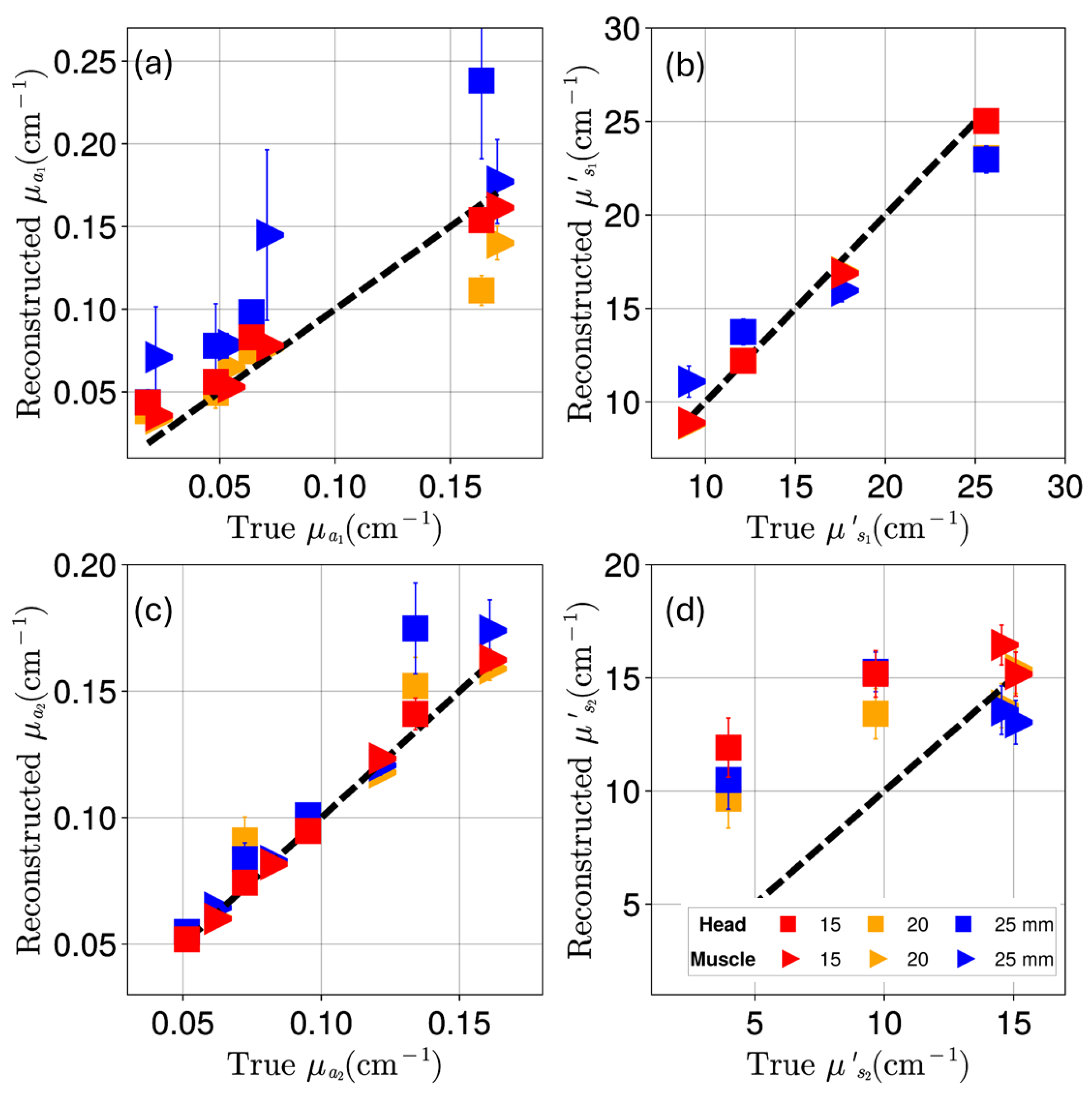
Figure A2.
True versus reconstructed transport coefficients at 850 nm.
Appendix C. Reconstruction of Deoxygenated and Oxygenated Hemoglobin Concentrations
Figure A3.
The reconstructed chromophore concentrations at 2 cm. Here, similar to Figure 3, the x-axis is not evenly spaced to avoid sparsely populated graph.
Figure A3.
The reconstructed chromophore concentrations at 2 cm. Here, similar to Figure 3, the x-axis is not evenly spaced to avoid sparsely populated graph.
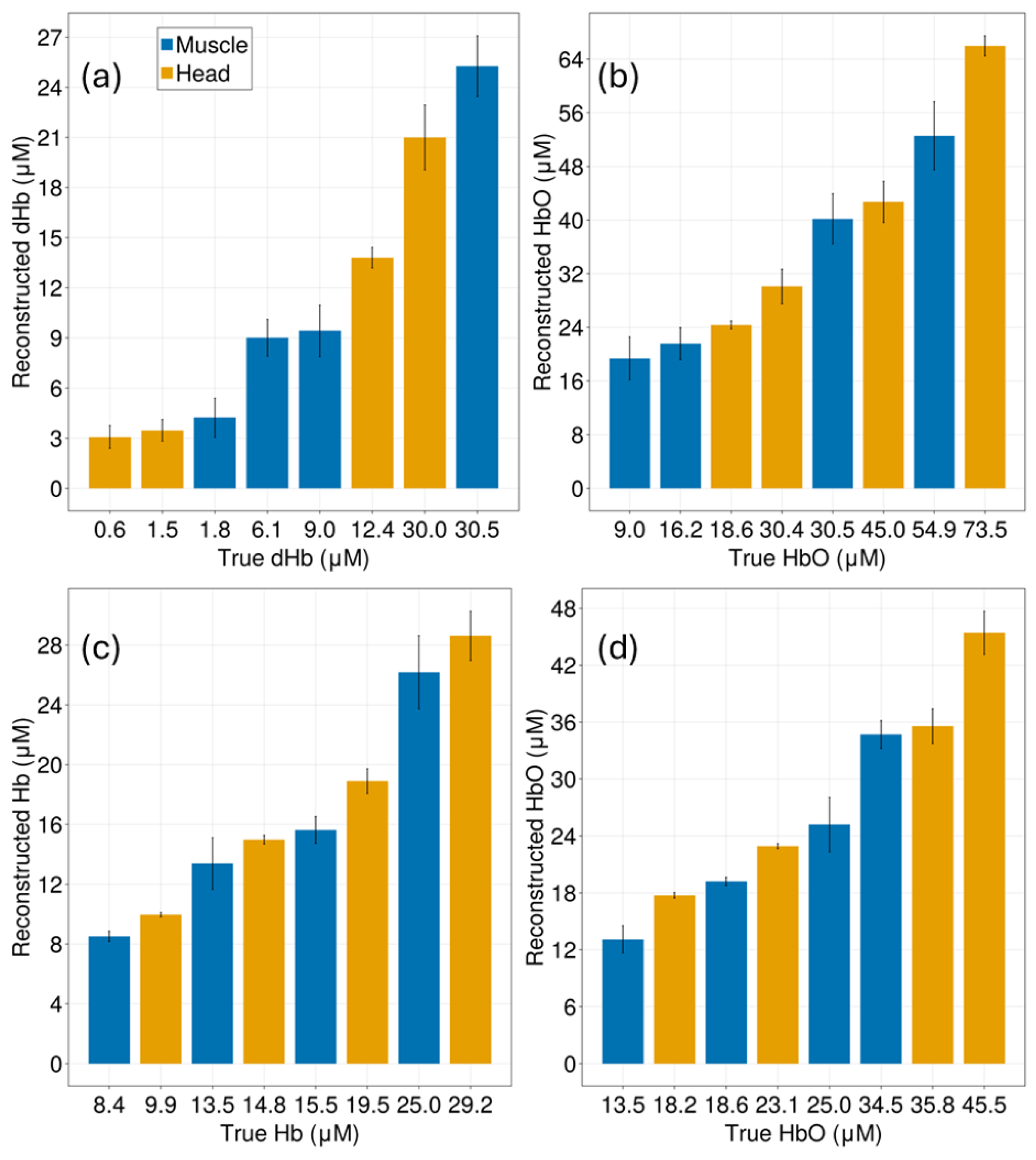
Figure A4.
The reconstructed chromophore concentration at 2.5 cm. The notable difference here being the increased error in retrieval of the top layer concentrations.
Figure A4.
The reconstructed chromophore concentration at 2.5 cm. The notable difference here being the increased error in retrieval of the top layer concentrations.
Appendix D. Reconstruction of Optical Coefficients Using Semi-Infinite Tissue Approximation
Semi
Figure A5.
Comparison of percent errors in the reconstructed optical properties for the bilayered and semi-infinite (SI) models. The sub-figures (a) and (b), correspond to SDS = 2 and 2.5 cm respectively. The optical properties analyzed include the absorption coefficients of the first and second layers (, ) and the reduced scattering coefficients of the first and second layers (, ) labeled as groups along the x-axis.
References
- Blaney, G.; Donaldson, R.; Mushtak, S.; Nguyen, H.; Vignale, L.; Fernandez, C.; Pham, T.; Sassaroli, A.; Fantini, S. Dual-Slope Diffuse Reflectance Instrument for Calibration-Free Broadband Spectroscopy. Applied Sciences 2021, 11. [Google Scholar] [CrossRef] [PubMed]
- Shimada, M.; Hoshi, Y.; Yamada, Y. Simple algorithm for the measurement of absorption coefficients of a two-layered medium by spatially resolved and time-resolved reflectance. Applied Optics 2005, 44, 7554. [Google Scholar] [CrossRef]
- Sekar, S.K.V.; Lanka, P.; Farina, A.; Mora, A.D.; Andersson-Engels, S.; Taroni, P.; Pifferi, A. Broadband Time Domain Diffuse Optical Reflectance Spectroscopy: A Review of Systems, Methods, and Applications. Applied Sciences 2019, Vol. 9, Page 5465 2019, 9, 5465. [Google Scholar] [CrossRef]
- Ugai, T.; Sasamoto, N.; Lee, H.Y.; Ando, M.; Song, M.; Tamimi, R.M.; Kawachi, I.; Campbell, P.T.; Giovannucci, E.L.; Weiderpass, E.; et al. Is early-onset cancer an emerging global epidemic? Current evidence and future implications. [CrossRef]
- Ferrari, M.; Quaresima, V. A brief review on the history of human functional near-infrared spectroscopy (fNIRS) development and fields of application. NeuroImage 2012, 63, 921–935. [Google Scholar] [CrossRef]
- Yamada, Y.; Suzuki, H.; Yamashita, Y. Time-Domain Near-Infrared Spectroscopy and Imaging: A Review. Applied Sciences 2019, 9. [Google Scholar] [CrossRef]
- Pifferi, A.; Contini, D.; Mora, A.D.; Farina, A.; Spinelli, L.; Torricelli, A. New frontiers in time-domain diffuse optics, a review. Journal of Biomedical Optics 2016, 21, 091310. [Google Scholar] [CrossRef]
- Boer, L.L.D.; Bydlon, T.M.; Duijnhoven, F.V.; Peeters, M.J.T.V.; Loo, C.E.; Winter-Warnars, G.A.; Sanders, J.; Sterenborg, H.J.; Hendriks, B.H.; Ruers, T.J. Towards the use of diffuse reflectance spectroscopy for real-time in vivo detection of breast cancer during surgery. Journal of Translational Medicine 2018, 16, 1–14. [Google Scholar] [CrossRef]
- Hallacoglu, B. Absolute measurement of cerebral optical coefficients, hemoglobin concentration and oxygen saturation in old and young adults with near-infrared spectroscopy. Journal of Biomedical Optics 2012, 17, 081406. [Google Scholar] [CrossRef] [PubMed]
- Farina, A.; Torricelli, A.; Bargigia, I.; Spinelli, L.; Cubeddu, R.; Foschum, F.; Jäger, M.; Simon, E.; Fugger, O.; Kienle, A.; et al. In-vivo multilaboratory investigation of the optical properties of the human head. Biomedical Optics Express 2015, 6, 2609. [Google Scholar] [CrossRef]
- Calcaterra, V.; Lacerenza, M.; Amendola, C.; Buttafava, M.; Contini, D.; Rossi, V.; Spinelli, L.; Zanelli, S.; Zuccotti, G.; Torricelli, A. Cerebral baseline optical and hemodynamic properties in pediatric population: a large cohort time-domain near-infrared spectroscopy study. Neurophotonics 2024, 11. [Google Scholar] [CrossRef]
- Bossi, A.; Bianchi, L.; Saccomandi, P.; Pifferi, A. Optical signatures of thermal damage on ex-vivo brain, lung and heart tissues using time-domain diffuse optical spectroscopy. Biomedical Optics Express 2024, 15, 2481. [Google Scholar] [CrossRef] [PubMed]
- Martelli, F.; Binzoni, T.; Bianco, S.D.; Liemert, A.; Kienle, A. Light Propagation Through Biological Tissue and Other Diffusive Media_ Theory, Solutions, and Validations; SPIE, 2022. [Google Scholar]
- Hoshi, Y. New Horizons in Time-Domain Diffuse Optical Spectroscopy and Imaging; MDPI, 2020. [Google Scholar]
- Blaney, G.; Sassaroli, A.; Fantini, S. Spatial sensitivity to absorption changes for various near-infrared spectroscopy methods: A compendium review. Journal of Innovative Optical Health Sciences 2024. [Google Scholar] [CrossRef]
- Wada, H.; Yoshizawa, N.; Ohmae, E.; Ueda, Y.; Yoshimoto, K.; Mimura, T.; Nasu, H.; Asano, Y.; Ogura, H.; Sakahara, H.; et al. Water and lipid content of breast tissue measured by six-wavelength time-domain diffuse optical spectroscopy. Journal of Biomedical Optics 2022, 27. [Google Scholar] [CrossRef]
- Tagliabue, S.; Kacprzak, M.; Rey-Perez, A.; Baena, J.; Riveiro, M.; Maruccia, F.; Fischer, J.B.; Poca, M.A.; Durduran, T. How the heterogeneity of the severely injured brain affects hybrid diffuse optical signals: case examples and guidelines. Neurophotonics 2024, 11. [Google Scholar] [CrossRef]
- Kienle, A.; Glanzmann, T.; Wagnières, G.; van den Bergh, H. Investigation of two-layered turbid media with time-resolved reflectance. Applied Optics 1998, 37, 6852. [Google Scholar] [CrossRef] [PubMed]
- Taroni, P.; Pifferi, A.; Quarto, G.; Farina, A.; Ieva, F.; Paganoni, A.M.; Abbate, F.; Cassano, E.; Cubeddu, R. Time domain diffuse optical spectroscopy: in-vivo quantification of collagen in breast tissue. In Proceedings of the Optical Methods for Inspection, Characterization, and Imaging of Biomaterials II; SPIE, 2015; Vol. 9529, pp. 140–147. [Google Scholar]
- Pellicer, A.; del Carmen Bravo, M. Near-infrared spectroscopy: A methodology-focused review. Seminars in Fetal and Neonatal Medicine 2011, 16, 42–49. [Google Scholar] [CrossRef] [PubMed]
- Vera, D.A.; García, H.A.; Waks-Serra, M.V.; Carbone, N.A.; Iriarte, D.I.; Pomarico, J.A. Determining light absorption changes in multilayered turbid media through analytically computed photon mean partial pathlengths. Optica Pura y Aplicada 2023, 56. [Google Scholar] [CrossRef]
- Hielscher, A.H.; Liu, H.; Chance, B.; Tittel, F.K.; Jacques, S.L. Time-resolved photon emission from layered turbid media. Applied Optics 1996, 35, 719. [Google Scholar] [CrossRef]
- Lanka, P.; Segala, A.; Farina, A.; Sekar, S.K.V.; Nisoli, E.; Valerio, A.; Taroni, P.; Cubeddu, R.; Pifferi, A. Non-invasive investigation of adipose tissue by time domain diffuse optical spectroscopy. Biomedical Optics Express 2020, 11, 2779. [Google Scholar] [CrossRef]
- Giovannella, M.; Contini, D.; Pagliazzi, M.; Pifferi, A.; Spinelli, L.; Erdmann, R.; Donat, R.; Rocchetti, I.; Rehberger, M.; Konig, N.; et al. BabyLux device: a diffuse optical system integrating diffuse correlation spectroscopy and time-resolved near-infrared spectroscopy for the neuromonitoring of the premature newborn brain. Neurophotonics 2019, 6, 1. [Google Scholar] [CrossRef]
- Jones, Z.D.; Reitzle, D.; Kienle, A. Errors in diffuse optical absorption spectroscopy of two-layered turbid media due to assuming a homogeneous medium. Opt. Lett. 2025, 50, 3118–3121. [Google Scholar] [CrossRef] [PubMed]
- Ferrari, M.; Quaresima, V. Near Infrared Brain and Muscle Oximetry: From the Discovery to Current Applications. Journal of Near Infrared Spectroscopy 2012, 20, 1–14. [Google Scholar] [CrossRef]
- Helton, M.; Zerafa, S.; Vishwanath, K.; Mycek, M.A. Efficient computation of the steady-state and time-domain solutions of the photon diffusion equation in layered turbid media. Sci. Rep. 2022, 12, 18979. [Google Scholar] [CrossRef] [PubMed]
- Jacques, S.L. Optical properties of biological tissues: a review. Physics in Medicine & Biology 2013, 58, R37. [Google Scholar] [CrossRef]
- Gagnon, L.; Gauthier, C.; Hoge, R.D.; Lesage, F.; Selb, J.; Boas, D.A. Double-layer estimation of intra- and extracerebral hemoglobin concentration with a time-resolved system. Journal of Biomedical Optics 2008, 13, 054019. [Google Scholar] [CrossRef]
- Shimada, M.; Hoshi, Y.; Yamada, Y. Simple algorithm for the measurement of absorption coefficients of a two-layered medium by spatially resolved and time-resolved reflectance. Appl. Opt. 2005, 44, 7554–7563. [Google Scholar] [CrossRef]
- Sato, C.; Shimada, M.; Yamada, Y.; Hoshi, Y. Extraction of depth-dependent signals from time-resolved reflectance in layered turbid media. Journal of Biomedical Optics 2005, 10, 064008. [Google Scholar] [CrossRef]
- Sharma, M.; Hennessy, R.; Markey, M.K.; Tunnell, J.W. Verification of a two-layer inverse Monte Carlo absorption model using multiple source-detector separation diffuse reflectance spectroscopy. Biomedical Optics Express 2014, 5, 40. [Google Scholar] [CrossRef]
- Blaney, G.; Bottoni, M.; Sassaroli, A.; Fernandez, C.; Fantini, S. Broadband diffuse optical spectroscopy of two-layered scattering media containing oxyhemoglobin, deoxyhemoglobin, water, and lipids. Journal of Innovative Optical Health Sciences 2022, 15. [Google Scholar] [CrossRef]
- Sato, C.; Shimada, M.; M.D., Y.H.; Yamada, Y. Extraction of depth-dependent signals from time-resolved reflectance in layered turbid media. Journal of Biomedical Optics 2005, 10, 064008. [Google Scholar] [CrossRef]
- Steinbrink, J.; Wabnitz, H.; Obrig, H.; Villringer, A.; Rinneberg, H. Determining changes in NIR absorption using a layered model of the human head. Physics in Medicine and Biology 2001, 46, 879–896. [Google Scholar] [CrossRef] [PubMed]
- Kienle, A.; Patterson, M.S.; Dögnitz, N.; Bays, R.; Wagnières, G.; van den Bergh, H. Noninvasive determination of the optical properties of two-layered turbid media. Applied Optics 1998, 37, 779. [Google Scholar] [CrossRef] [PubMed]
- Kienle, A.; Patterson, M.S. Improved solutions of the steady-state and the time-resolved diffusion equations for reflectance from a semi-infinite turbid medium. Journal of the Optical Society of America A 1997, 14, 246. [Google Scholar] [CrossRef]
- Tualle, J.M.; Prat, J.; Tinet, E.; Avrillier, S. Real-space Green’s function calculation for the solution of the diffusion equation in stratified turbid media. Journal of the Optical Society of America A 2000, 17, 2046. [Google Scholar] [CrossRef]
- Martelli, F.; Pifferi, A.; Farina, A.; Amendola, C.; Maffeis, G.; Tommasi, F.; Cavalieri, S.; Spinelli, L.; Torricelli, A. Statistics of maximum photon penetration depth in a two-layer diffusive medium. Biomedical Optics Express 2024, 15, 1163. [Google Scholar] [CrossRef] [PubMed]
- Martelli, F.; Sassaroli, A.; Yamada, Y.; Zaccanti, G. Analytical approximate solutions of the time-domain diffusion equation in layered slabs. Journal of the Optical Society of America. A, Optics, image science, and vision 2002, 19 1, 71–80. [Google Scholar] [CrossRef]
- García, H.; Iriarte, D.; Pomarico, J.; Grosenick, D.; Macdonald, R. Retrieval of the optical properties of a semiinfinite compartment in a layered scattering medium by single-distance, time-resolved diffuse reflectance measurements. Journal of Quantitative Spectroscopy and Radiative Transfer 2017, 189, 66–74. [Google Scholar] [CrossRef]
- Wu, M.M.; Chan, S.T.; Mazumder, D.; Tamborini, D.; Stephens, K.A.; Deng, B.; Farzam, P.; Chu, J.Y.; Franceschini, M.A.; Qu, J.Z.; et al. Improved accuracy of cerebral blood flow quantification in the presence of systemic physiology cross-talk using multi-layer Monte Carlo modeling. Neurophotonics 2021, 8. [Google Scholar] [CrossRef]
- Martelli, F.; Sassaroli, A.; Bianco, S.D.; Yamada, Y.; Zaccanti, G. Solution of the time-dependent diffusion equation for layered diffusive media by the eigenfunction method. Physical Review E 2003, 67, 056623. [Google Scholar] [CrossRef]
- Helton, M. LightPropagation.jl: A Julia package for simulating light propagation, 2025. Accessed: 2025-03-15.
- McMurdy, J.; Jay, G.; Suner, S.; Crawford, G. Photonics-based In Vivo total hemoglobin monitoring and clinical relevance. Journal of Biophotonics 2009, 2, 277–287. [Google Scholar] [CrossRef]
- Prahl, S. Optical Absorption Spectra of Hemoglobin. https://omlc.org/spectra/hemoglobin/summary.html, 1999. Accessed: October 15, 2023. Oregon Medical Laser Center.
- Vishwanath, K.; Pogue, B.; Mycek, M.A. Quantitative fluorescence lifetime spectroscopy in turbid media: comparison of theoretical, experimental and computational methods. Physics in Medicine & Biology 2002, 47, 3387. [Google Scholar] [CrossRef]
- Vishwanath, K.; Mycek, M.A. Time-resolved photon migration in bi-layered tissue models. Optics Express 2005, 13, 7466. [Google Scholar] [CrossRef] [PubMed]
- Khan, R.; Gul, B.; Khan, S.; Nisar, H.; Ahmad, I. Refractive index of biological tissues: Review, measurement techniques, and applications. Photodiagnosis and Photodynamic Therapy 2021, 33, 102192. [Google Scholar] [CrossRef]
- Martelli, F.; Bianco, S.D.; Zaccanti, G.; Pifferi, A.; Torricelli, A.; Bassi, A.; Taroni, P.; Cubeddu, R. Phantom validation and in vivo application of an inversion procedure for retrieving the optical properties of diffusive layered media from time-resolved reflectance measurements. Optics Letters 2004, 29, 2037. [Google Scholar] [CrossRef] [PubMed]
- Rajasekhar, S.; Vishwanath, K. Sensitivity Of Time-Resolved Diffuse Reflectance To Optical Coefficients In Bilayered Tissues. In Proceedings of the Frontiers in Optics + Laser Science 2024 (FiO, LS); Optica Publishing Group, 2024; p. JW5A.45. [Google Scholar] [CrossRef]
- Stawschenko, E.; Schaller, T.; Kern, B.; Bode, B.; Dörries, F.; Kusche-Vihrog, K.; Gehring, H.; Wegerich, P. Current Status of Measurement Accuracy for Total Hemoglobin Concentration in the Clinical Context. Biosensors 2022, 12. [Google Scholar] [CrossRef]
- Nasseri, N.; Kleiser, S.; Ostojic, D.; Karen, T.; Wolf, M. Quantifying the effect of adipose tissue in muscle oximetry by near infrared spectroscopy. Biomedical Optics Express 2016, 7, 4605. [Google Scholar] [CrossRef]
- Dehaes, M.; Grant, P.E.; Sliva, D.D.; Roche-Labarbe, N.; Pienaar, R.; Boas, D.A.; Franceschini, M.A.; Selb, J. Assessment of the frequency-domain multi-distance method to evaluate the brain optical properties: Monte Carlo simulations from neonate to adult. Biomedical Optics Express 2011, 2, 552. [Google Scholar] [CrossRef]
Figure 1.
(a) illustrates two-layer models for head and limb tissues. Each layer is represented as a cylinder having the same radius, but different thickness. All models used had fixed upper layer thickness of 1 cm. Tissue media were characterized the absorption (, ) and reduced scattering coefficients (, ), where layer 1 was the top layer. (b) time-resolved reflectance from a muscle tissue model obtained using MC (symbols), forward DT calculations (solid lines) and from inverse-fits (dashed lines) at SDS cm. Colors represent data for the same tissue model at three wavelengths used (indigo: 690 nm, orange: 760 nm and red: 850 nm).
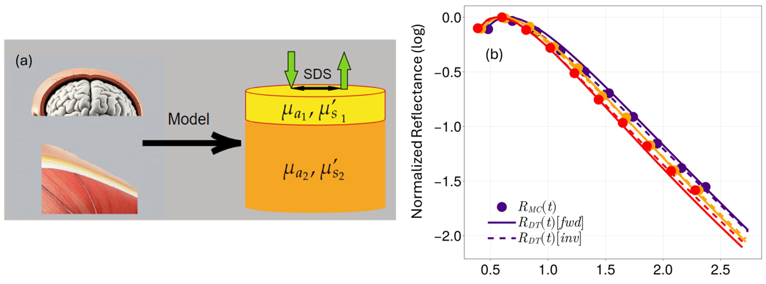
Figure 2.
True versus reconstructed optical coefficients at 760 nm for absorption ( and in (a) and (c)) and reduced scattering coefficients (, in (b) and (d)) across each of the 64 models for brain (squares) and the 64 models for muscle (triangles). Colors represent different SDS: red for cm, orange for 2 cm and blue for cm and the dashed black line represents the line. The error bars represent the standard error across all models that share fixed values of each optical coefficient under investigation. It is important to note that there are six different markers each with its own error bar. Many of the error bars are smaller than the marker sizes used.
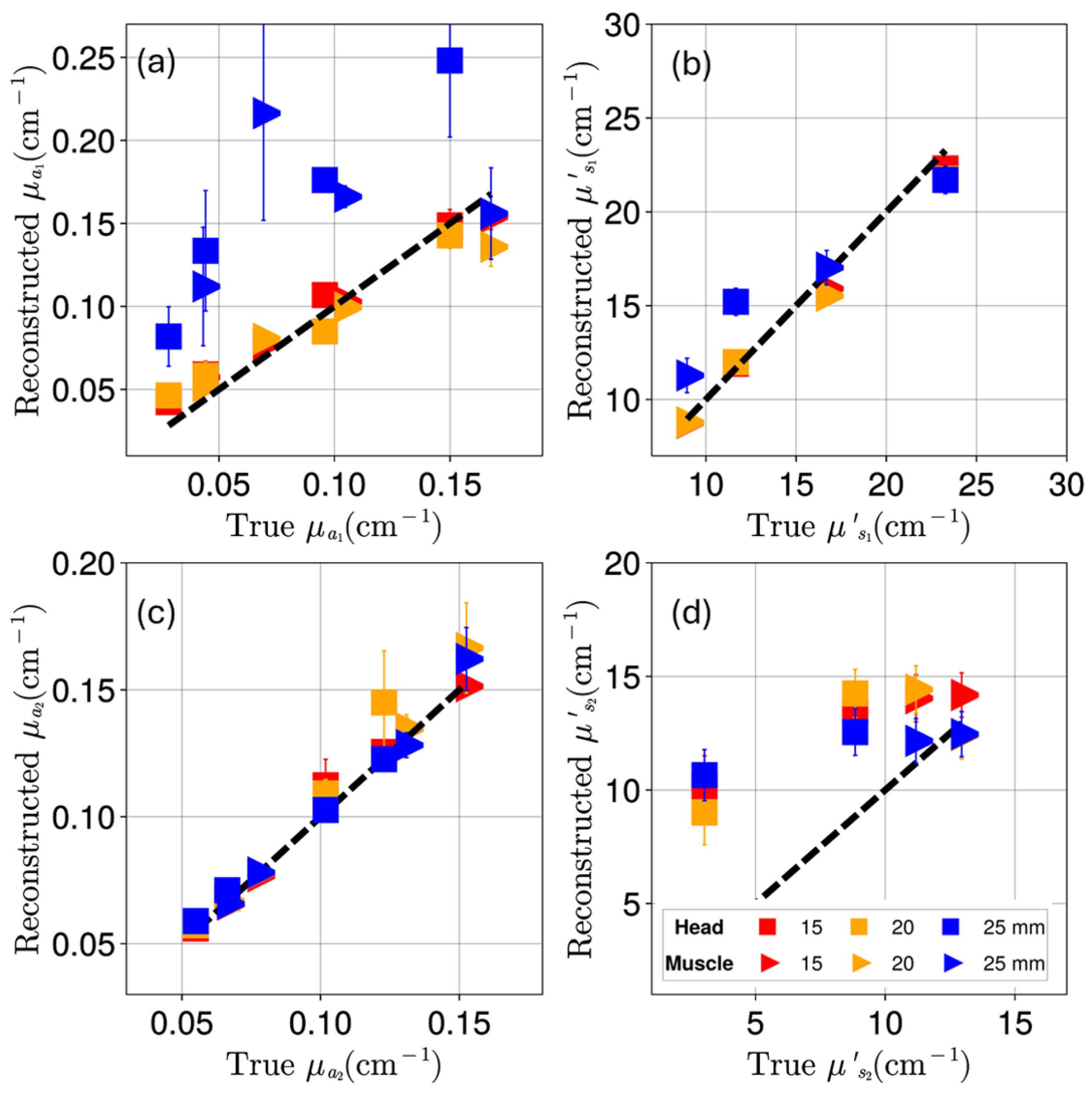
Figure 3.
Reconstructed and concentrations for muscle (blue) and brain (orange) at an SDS of 1.5 cm. The x-axis represents the true hemoglobin concentrations (not evenly spaced) computed from the model values derived from Table 1. While the y-axis shows the reconstructed (median) values. Subplots (a) and (b) represent the top layer and (c) and (d), the bottom layer reconstruction of and respectively. Each data bar in each plot represents sixteen models and the error-bar is the standard error across the models.
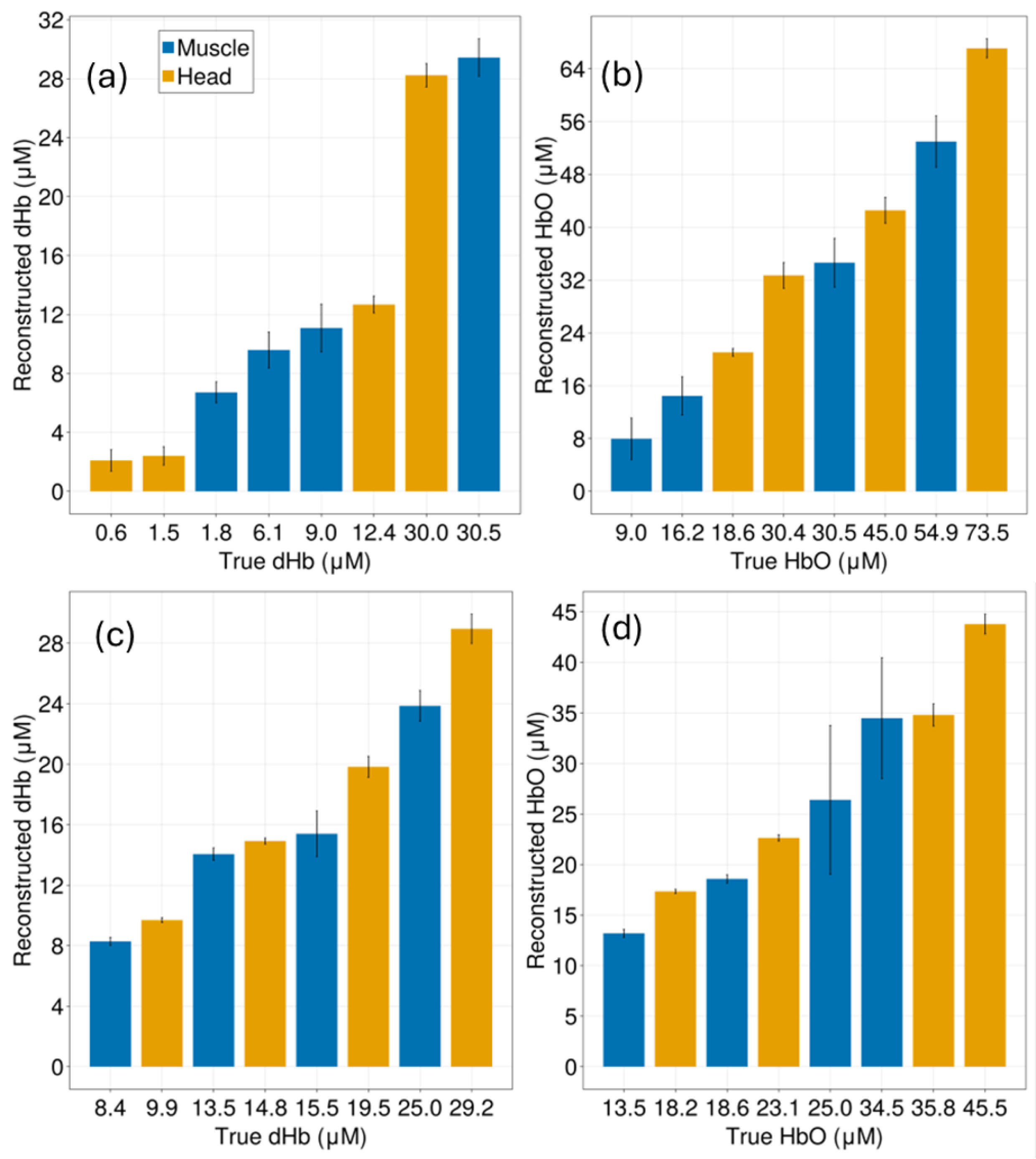
Figure 4.
Reconstruction accuracy of and for different source-detector SDS in a two-layer model. (a) and (b) show the reconstructed (median) versus true values of and , respectively, for the top layer, while (c) and (d) display the same for the bottom layer. The colors represent different SDS values: mm (red), 2 mm (orange), and mm (blue). The dash black line represents the line. The reconstruction for the top layer showed poor accuracy while the bottom layer reconstruction showed much better reconstructions, highlighting the effectiveness of DT to probe deeper tissue layers. These data were computed using reconstructed and values.
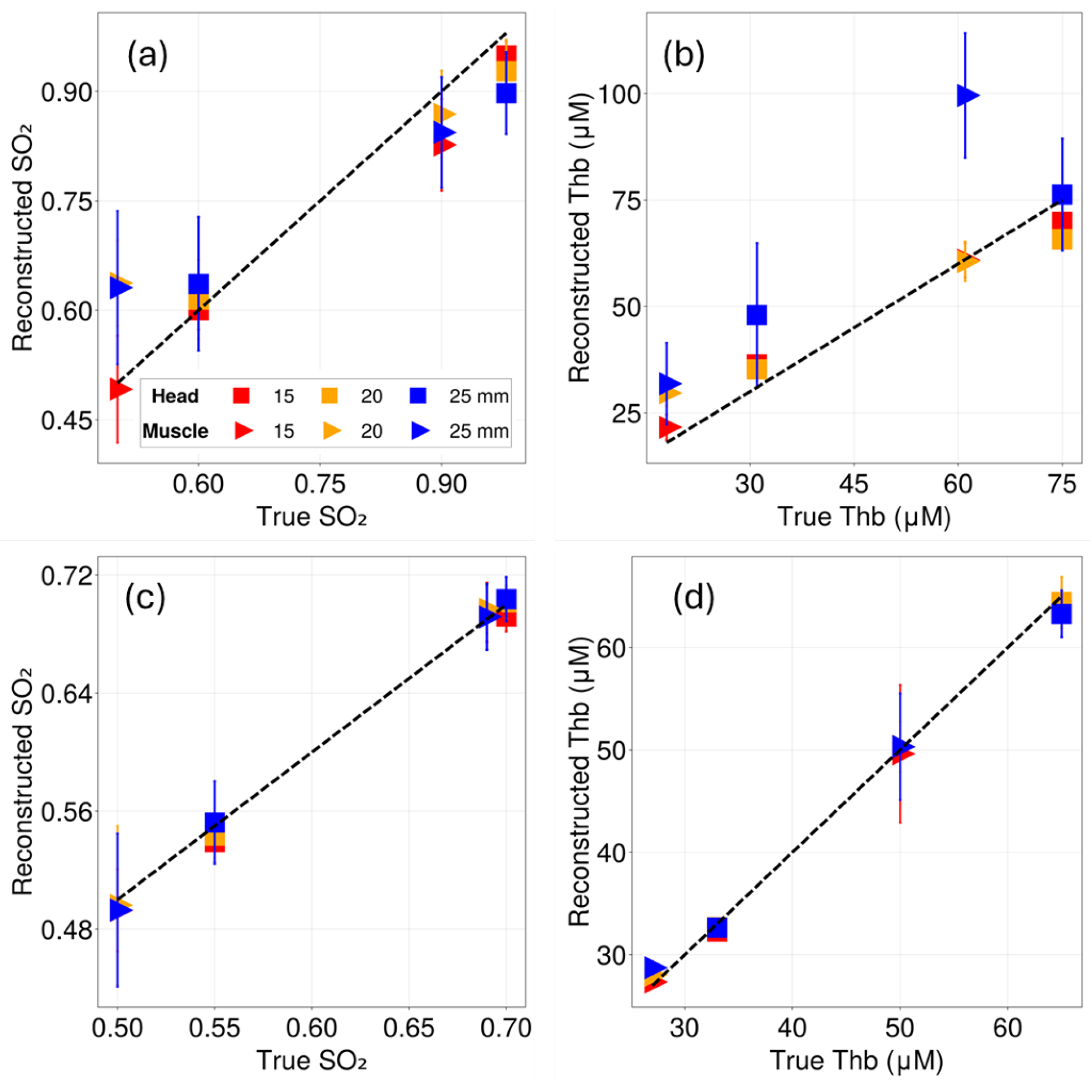
Figure 5.
Comparison of median percent error in reconstructed transport coefficients of bilayered media using a semi-infinite DT model. Each orange bar represents the median percent error in reconstructed absorption and scattering obtained from inverse SI DT model across the 384 bi-layered while the true value for each of the four coefficients (indicated by the axis labels) were those used to simulate . Error bars indicate the standard errors across the 384 models. The blue bars indicate these errors when reconstructions were done by using bilayered DT.
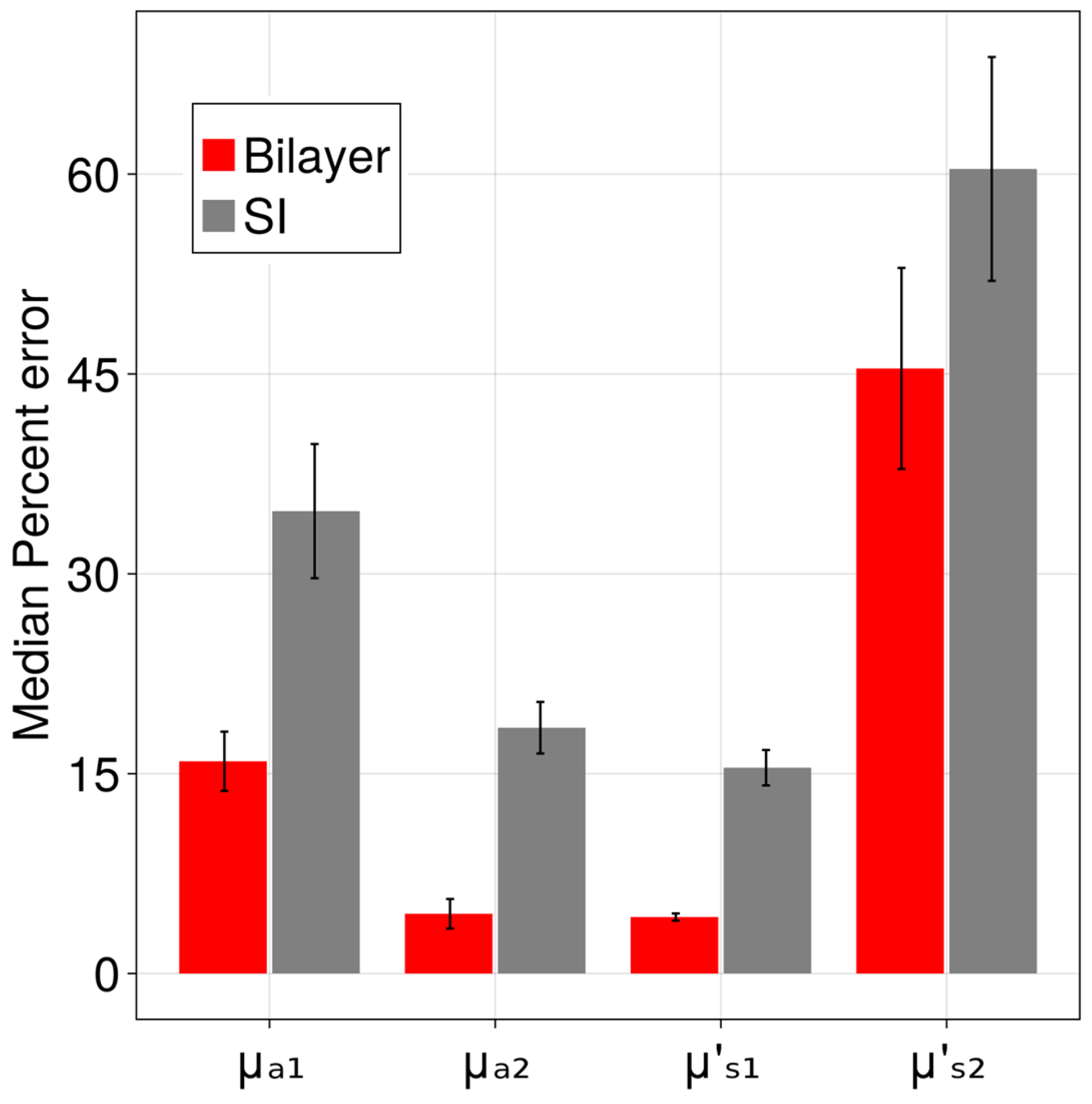
Table 1.
Input parameters used to generate optical coefficients of each layer. Two and values were used for the top and bottom layers, along with two different values of A and b for the top and bottom layers. A total of 64 different models were generated at any one wavelength.
Table 1.
Input parameters used to generate optical coefficients of each layer. Two and values were used for the top and bottom layers, along with two different values of A and b for the top and bottom layers. A total of 64 different models were generated at any one wavelength.
| Tissue Model | Layer | b | |||
|---|---|---|---|---|---|
| Head | Top | ||||
| Bottom | |||||
| Muscle | Top | ||||
| Bottom |
Disclaimer/Publisher’s Note: The statements, opinions and data contained in all publications are solely those of the individual author(s) and contributor(s) and not of MDPI and/or the editor(s). MDPI and/or the editor(s) disclaim responsibility for any injury to people or property resulting from any ideas, methods, instructions or products referred to in the content. |
© 2025 by the authors. Licensee MDPI, Basel, Switzerland. This article is an open access article distributed under the terms and conditions of the Creative Commons Attribution (CC BY) license (http://creativecommons.org/licenses/by/4.0/).
Copyright: This open access article is published under a Creative Commons CC BY 4.0 license, which permit the free download, distribution, and reuse, provided that the author and preprint are cited in any reuse.


