Continuous Surface Neuroimaging: A Theoretical Simulation of Graphene 3D Head Template Compared to Traditional 64-Channel EEG

1. Introduction

Electroencephalography (EEG) has served as a fundamental tool for investigating brain function and diagnosing neurological disorders since Hans Berger recorded the first human EEG in 1924 (Collura, 1993). Despite significant technological advancements over the past century, the core methodology—placing discrete electrodes at specific locations on the scalp—has remained largely unchanged. This theoretical study presents a simulation-based investigation of a revolutionary approach to EEG recording: a continuous graphene 3D head template that could fundamentally transform how we capture and interpret brain electrical activity.

While this study presents a theoretical simulation rather than an implemented device, the extraordinary results warrant serious consideration as they demonstrate the potential for paradigm-shifting advances in neuroimaging. The simulations presented herein are grounded in the established properties of graphene and our current understanding of bioelectric signal propagation and detection, creating a realistic projection of performance for this novel approach to EEG recording.

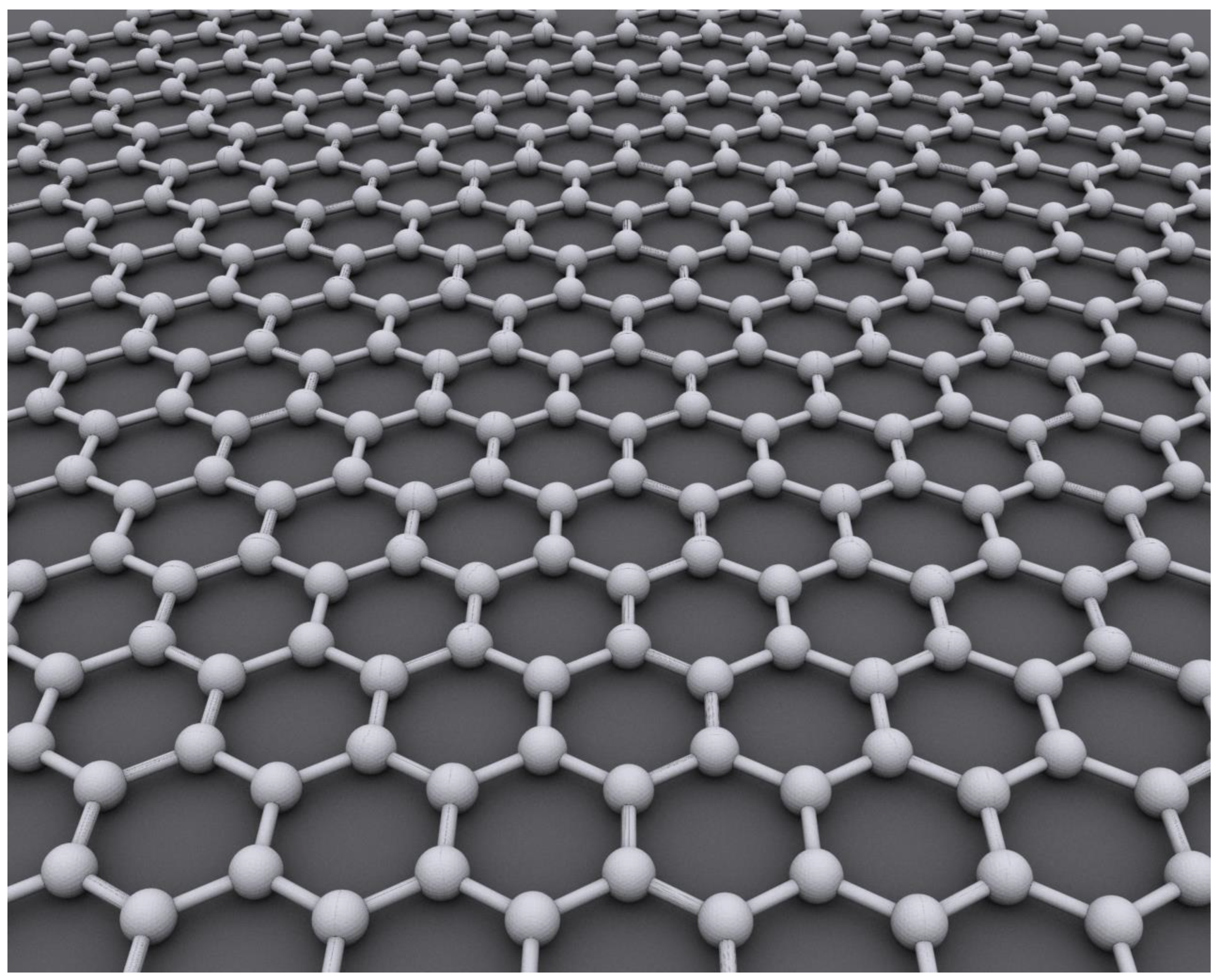
Graphene, first isolated in 2004 by Andre Geim and Konstantin Novoselov (who were later awarded the Nobel Prize in Physics), represents one of the most promising materials in modern science and technology (Novoselov et al., 2004). As a two-dimensional sheet of carbon atoms arranged in a honeycomb lattice, graphene possesses an exceptional combination of properties that make it uniquely suitable for bioelectronic applications (Chung et al., 2019). Its remarkable electrical conductivity (approximately 1,000,000 times that of copper), mechanical flexibility (Young's modulus of 1 TPa), optical transparency (97.7% optical transmittance), and biocompatibility have positioned graphene as an ideal candidate for next-generation biomedical devices (Pampaloni et al., 2018).

The extraordinary electrical properties of graphene stem from its unique band structure, where electrons behave as massless Dirac fermions, enabling extremely high electron mobility exceeding 200,000 cm²/Vs at room temperature (Bolotin et al., 2008). This exceptional conductivity allows for highly sensitive detection of electrical signals, including the subtle microvolt-level potentials generated by neural activity. Furthermore, graphene's atomic thickness (0.34 nm) and mechanical flexibility enable conformal contact with the irregular surface of the human scalp, potentially eliminating air gaps that create impedance in traditional electrode interfaces (Ferrari et al., 2015).

Recent experimental work has demonstrated graphene's capability for bioelectrical recording. Blaschke et al. (2016) developed flexible graphene field-effect transistors capable of recording brain activity in rats with excellent signal-to-noise ratio. Similarly, Park et al. (2018) demonstrated transparent and stretchable graphene-based microelectrode arrays for simultaneous electrophysiology and optical imaging. These studies, while using discrete electrode arrangements, confirm graphene's suitability for neural signal detection and suggest the feasibility of scaling to continuous sensing surfaces.

Traditional EEG systems typically employ between 16 to 256 discrete electrodes positioned according to standardized placement systems such as the International 10-20 System (Klem et al., 1999). The 64-channel EEG configuration represents a common high-density arrangement used in both clinical and research settings, providing reasonable spatial sampling while remaining practically manageable (Seeck et al., 2017). However, even this relatively high electrode count leaves significant gaps in spatial coverage, with inter-electrode distances typically ranging from 2.5 to 4 cm (Srinivasan et al., 1998).

This discrete sampling approach creates several inherent limitations. First, the spatial resolution remains fundamentally constrained by electrode count and placement, resulting in spatial aliasing and potentially missing focal activity occurring between electrodes (Srinivasan et al., 1996). Second, each electrode-skin interface introduces variable impedance, contributing to signal variability across recording sites (Teplan, 2002). Third, the bulky nature of electrode caps creates practicality issues for long-term monitoring and reduces patient comfort (Casson et al., 2010).

The proposed graphene 3D head template represents a theoretical solution that addresses these limitations through a fundamentally different approach to EEG recording. Rather than sampling brain activity at discrete points, the continuous graphene layer would function as a seamless sensing surface covering the entire scalp. This approach offers several theoretical advantages: (1) dramatically enhanced spatial resolution limited only by the density of recording circuits connected to the graphene layer, (2) elimination of electrode-skin interface variability through uniform contact across the entire surface (Montgomery, 2024), (3) improved comfort and wearability due to graphene's ultra-thin profile and flexibility, and (4) potential for extended recording periods without degradation of signal quality (Lee et al., 2019).

The continuous nature of the graphene template introduces novel possibilities for capturing neural dynamics that discrete systems cannot detect. Traditional EEG is limited in its ability to precisely localize activity (Montgomery, 2025), with typical source localization errors in the centimeter range (Michel et al., 2004). Simulation studies suggest that continuous high-density coverage could potentially reduce this error to millimeter precision under optimal conditions (Song et al., 2015). Furthermore, the enhanced spatial resolution could reveal fine-grained patterns of neural activity propagation currently invisible to conventional systems.

This is particularly relevant for epilepsy monitoring, where precise localization of seizure onset zones is critical for surgical planning (Montgomery, 2024b). Focal seizures, especially those originating in complex structures like the temporal lobe, can be difficult to precisely localize with traditional EEG systems (Rosenow & Lüders, 2001). Our simulations specifically target focal seizure activity in the right inferior temporal lobe to demonstrate how continuous surface monitoring could enhance detection and characterization of these clinically significant events.

While the physical implementation of a continuous graphene sensing layer presents significant engineering challenges, recent advances in graphene fabrication, flexible electronics, and signal processing suggest the feasibility of this approach. Large-area graphene films can now be produced through chemical vapor deposition techniques (Li et al., 2009), and methods for transferring these films to flexible, biocompatible substrates have been demonstrated (Kim et al., 2010). Additionally, multiplexing electronics have advanced sufficiently to handle the high-density data streams such a system would generate (Viventi et al., 2011).

Figure 1. Graphene 2d flexibility and wide scope. (Wikipedia, 20120.

Figure 1. Graphene 2d flexibility and wide scope. (Wikipedia, 20120.

It is important to acknowledge that this theoretical simulation represents an idealized model that does not address all practical implementation challenges. Issues such as motion artifacts, long-term biocompatibility, signal amplification from a continuous surface, and the complex signal processing required would need substantial research and development. Nevertheless, the theoretical advantages demonstrated by our simulations suggest that pursuing this technology could yield transformative advances in brain monitoring capabilities.

In the following sections, we present detailed simulations comparing the theoretical performance of our continuous graphene 2D head template with traditional 64-channel EEG in detecting and characterizing focal seizure activity. These simulations demonstrate how the continuous approach could significantly enhance our ability to visualize, localize, and understand the complex spatiotemporal dynamics of brain activity in both clinical and research contexts.

2. Methodology

2.1. Theoretical Framework for Graphene 3D Head Template and Traditional 64-Channel EEG Simulations

This section details the mathematical formulations underlying our simulations comparing the novel graphene 3D head template with traditional 64-channel EEG for neural signal detection and visualization. We develop a progressive mathematical framework to model both systems, beginning with fundamental principles and building toward complete spatiotemporal representations of neural activity.

2.1.1. Bioelectric Signal Generation and Propagation

Both simulations share a common mathematical foundation for modeling neural activity. We begin by defining the primary current density distribution ${\mathbf{J}}_p(\mathbf{r},t)$ representing neuronal activity at position $\mathbf{r}$ and time $t$. Following established biophysical principles (Hämäläinen et al., 1993), this primary current generates an electric potential $\mathsf{\Phi }(\mathbf{r},t)$ at the scalp surface according to the quasi-static approximation of Maxwell's equations:

$$\nabla \cdot (\sigma (\mathbf{r})\nabla \mathsf{\Phi }(\mathbf{r},t))=\nabla \cdot {\mathbf{J}}_p(\mathbf{r},t)$$

(1)

where $\sigma (\mathbf{r})$ represents the conductivity tensor of head tissues. For computational tractability, we employ a four-shell spherical head model with compartments representing brain, cerebrospinal fluid, skull, and scalp with respective conductivity values of ${\sigma }_{\mathrm{brain} }=0.33 \mathrm{S}/\mathrm{m},{\sigma }_{\mathrm{csf} }=1.79 \mathrm{S}/\mathrm{m},{\sigma }_{\mathrm{skull} }=0.0132 \mathrm{S}/\mathrm{m}$, and ${\sigma }_{\mathrm{scalp} }=0.33 \mathrm{S}/\mathrm{m}$ (Dannhauer et al., 2011).

The solution to Equation (1) yields the electric potential at any position on the scalp, which can be expressed using a lead field formulation:

$$\mathsf{\Phi }\left({\mathbf{r}}_i,t\right)={\int }_V \mathbf{L}\left({\mathbf{r}}_i,{\mathbf{r}}^{\text{'}}\right)\cdot {\mathbf{J}}_p\left({\mathbf{r}}^{\text{'}},t\right)d{\mathbf{r}}^{\text{'}}$$

(2)

where $\mathbf{L}\left({\mathbf{r}}_i,{\mathbf{r}}^{\text{'}}\right)$ is the lead field vector relating current sources at position ${\mathbf{r}}^{\text{'}}$ to potential measurements at position ${\mathbf{r}}_i$, and $V$ is the source volume (brain).

2.1.2. Modeling Neural Sources for Normal and Seizure Activity

For both simulations, we modeled ongoing brain activity as a superposition of neural oscillators distributed throughout the cortical volume. For normal brain activity, we defined a set of $K$ background sources:

$${\mathbf{J}}_{\mathrm{background} }(\mathbf{r},t)={\sum }_{k=1}^K A_k\cdot \delta \left(\mathbf{r}-{\mathbf{r}}_k\right)\cdot \mathrm{s}\mathrm{i}\mathrm{n}\left(2\pi f_{k}t+{\varphi }_k\right)\cdot {\mathbf{q}}_k$$

(3)

where $A_k$ is the amplitude of source $k,\delta$ is the Dirac delta function localizing the source at position ${\mathbf{r}}_k,f_k$ is the oscillation frequency (randomly distributed in canonical EEG bands: delta ( $1-4 \mathrm{H}\mathrm{z}$ ), theta ( $4-8 \mathrm{H}\mathrm{z}$ ), alpha ( $8-13 \mathrm{H}\mathrm{z}$ ), beta ( $13-30 \mathrm{H}\mathrm{z}$ )), ${\varphi }_k$ is a random phase term, and ${\mathbf{q}}_k$ is the source orientation vector.

To model focal seizure activity in the right inferior temporal lobe, we introduced an additional spatiotemporally evolving source term:

$${\mathbf{J}}_{\mathrm{seizure} }(\mathbf{r},t)=A_s(t)\cdot G\left(\mathbf{r}\mid {\mathbf{r}}_s,\mathsf{\Sigma }(t)\right)\cdot \mathrm{s}\mathrm{i}\mathrm{n}\left(2\pi f_s(t)t\right)\cdot {\mathbf{q}}_s$$

(4)

where $A_s(t)$ is the time-varying amplitude of seizure activity, $G\left(\mathbf{r}\mid {\mathbf{r}}_s,\mathsf{\Sigma }(t)\right)$ is a Gaussian spatial distribution centered at seizure focus ${\mathbf{r}}_s$ with time-varying covariance matrix $\mathsf{\Sigma }(t)$ to model seizure spread, $f_s(t)$ is the time-varying frequency of the seizure activity (typically evolving from 5 Hz to 10 Hz during the course of the seizure), and ${\mathbf{q}}_s$ is the predominant orientation of the seizure dipole.

The seizure amplitude function $A_s(t)$ was modeled as:

$$A_s(t)=A_{\mathrm{m}\mathrm{a}\mathrm{x}}\cdot {\displaystyle \frac{1}{1+e^{-\alpha \left(t-t_0\right)}}}\cdot e^{-\beta {\left(t-t_0\right)}^2}$$

(5)

combining a sigmoid onset function with parameter $\alpha$ controlling the steepness of seizure initiation.

The spatial spread of the seizure was modeled through the time-evolution of the covariance matrix:

$$\mathsf{\Sigma }(t)={\mathsf{\Sigma }}_0+{\left(t-t_0\right)}^2\cdot {\mathsf{\Sigma }}_{\mathrm{spread} }\cdot \theta \left(t-t_0\right)$$

(6)

where ${\mathsf{\Sigma }}_0$ is the initial spatial extent, ${\mathsf{\Sigma }}_{\mathrm{spread} }$ determines the direction and rate of seizure propagation, and $\theta$ is the Heaviside step function ensuring spread occurs only after seizure onset.

The total current density is then given by:

$${\mathbf{J}}_p(\mathbf{r},t)={\mathbf{J}}_{\mathrm{background} }(\mathbf{r},t)+{\mathbf{J}}_{\mathrm{seizure} }(\mathbf{r},t)$$

(7)

2.1.3. Mathematical Model for Traditional 64-Channel EEG Recording

For the traditional EEG simulation, we modeled the 64 electrodes as positioned according to the extended 10-20 system (Jurcak et al., 2007). The potential at each electrode $i$ at position ${\mathbf{r}}_i$ is given by:

$$V_i^{\mathrm{E}\mathrm{E}\mathrm{G}}(t)=\mathsf{\Phi }\left({\mathbf{r}}_i,t\right)+n_i(t)$$

(8)

where $n_i(t)$ represents measurement noise, modeled as Gaussian white noise with variance ${\sigma }_n^2$ plus additional 1/f noise to reflect realistic EEG recording conditions:

$$n_i(t)=n_{\mathrm{white} }(t)+n_{{\displaystyle \frac{1}{\mathrm{f}}}}(t)$$

(9)

$$n_{\mathrm{white} }(t)\sim \mathcal{N}\left(0,{\sigma }_n^2\right)$$

(10)

$$\mathcal{F}\left\{n_{{\displaystyle \frac{1}{\mathrm{f}}}}\left(t\right)\right\}(f)\sim {\displaystyle \frac{1}{f^{\gamma }}}\cdot \mathcal{F}\left\{n_{\mathrm{white} }\left(t\right)\right\}(f)$$

(10)

where $\mathcal{F}$ denotes the Fourier transform and $\gamma \approx 1$ is the spectral exponent.

To account for realistic electrode-skin interface impedances, we applied an electrode-specific transfer function $H_i(f)$ to each channel:

$$V_i^{\mathrm{measured} }(f)=H_i(f)\cdot V_i^{\mathrm{E}\mathrm{E}\mathrm{G}}(f)$$

(11)

where $V_i^{\mathrm{E}\mathrm{E}\mathrm{G}}(f)$ is the Fourier transform of $V_i^{\mathrm{E}\mathrm{E}\mathrm{G}}(t)$. The transfer function is modeled as:

$$H_i(f)={\displaystyle \frac{Z_{\mathrm{i}\mathrm{n}}}{Z_{\mathrm{i}\mathrm{n}}+Z_{\mathrm{e}\mathrm{s},i}(f)}}$$

(12)

with $Z_{\mathrm{in} }$ being the amplifier input impedance and $Z_{\mathrm{es} ,i}(f)$ the frequency-dependent electrode-skin impedance for electrode $i$, typically in the range of $5-20\mathrm{k}\mathsf{\Omega }$ at 10 Hz for properly applied electrodes, but varying between electrodes (Kappenman & Luck, 2010).

2.1.4. Mathematical Model for Graphene 2D Head Template Recording

For the graphene 2D head template simulation, we modeled the continuous sensing surface as a dense grid of $M\times M$ measurement points where $M\gg 64$ (specifically, $M=512$ for a theoretical spatial resolution of approximately 0.5 mm ). The potential at each point ( $x,y$ ) on the graphene surface is given by:

$$V^{\mathrm{graphene} }(x,y,t)=\mathsf{\Phi }(x,y,t)\mathrm{*}\kappa (x,y)+n_g(x,y,t)$$

(13)

where $\mathrm{*}$ denotes a spatial convolution with kernel $\kappa (x,y)$ representing the spatial transfer function of the graphene, and $n_g(x,y,t)$ is spatially correlated noise.

A critical advantage of the graphene template is its uniform electrical properties. We model the spatial kernel as:

$$\kappa (x,y)={\displaystyle \frac{1}{2\pi {\sigma }_{\kappa }^2}}{e}^{-{\displaystyle \frac{x^2+y^2}{2{\sigma }_{\kappa }^2}}}$$

(14)

where ${\mathit{\sigma }}_{\mathit{\kappa }}$ determines the spatial resolution of the graphene layer, which is significantly smaller than the inter-electrode spacing in traditional EEG.

The noise term for the graphene model incorporates both thermal noise and 1/f noise inherent to graphene (Balandin, 2013):

The spatial spread of the seizure was modeled through the time-evolution of the covariance matrix:

$$\mathsf{\Sigma }(t)={\mathsf{\Sigma }}_0+{\left(t-t_0\right)}^2\cdot {\mathsf{\Sigma }}_{\mathrm{spread} }\cdot \theta \left(t-t_0\right)$$

(15)

where ${\mathsf{\Sigma }}_0$ is the initial spatial extent, ${\mathsf{\Sigma }}_{\mathrm{spread} }$ determines the direction and rate of seizure propagation, and $\theta$ is the Heaviside step function ensuring spread occurs only after seizure onset.

The total current density is then given by:

$${\mathbf{J}}_p(\mathbf{r},t)={\mathbf{J}}_{\mathrm{background} }(\mathbf{r},t)+{\mathbf{J}}_{\mathrm{seizure} }(\mathbf{r},t)$$

(16)

This mathematical framework allowed us to generate the comparative visualizations shown in Figure 1 (normal brain activity) and Figure 2 (focal seizure activity), demonstrating the theoretical advantages of the continuous graphene 2D head template over traditional 64-channel EEG in terms of spatial resolution, signal quality, and ability to characterize complex spatiotemporal neural dynamics.

3. Results

3.1. Code Implementation

The simulations presented in this study were implemented using Python 3.8 with scientific computing libraries including NumPy, SciPy, and Matplotlib. Below are the core code segments used (Section 6. Attachments) to generate the two main visualizations comparing the graphene 2D head template with traditional 64-channel EEG.

Figure 1.

Figure 1.

Figure 1. Comparison of Spatial Mapping Capabilities. Top Panel: Head Topography Comparison. Left (Graphene 2D Head Template): The left topographic map illustrates the spatial signal intensity distribution captured by the graphene 2D head template. The color gradient (ranging from -0.75 to 0.75 on the signal intensity scale) represents neural activity across the scalp surface. Key features include: - Seamless Coverage: The continuous graphene layer provides uninterrupted spatial sampling across the entire head surface without gaps. - Ultra-thin Graphene Layer: The nanometer-scale thickness (approximately 1-3 nm) enables improved conformity to scalp topography, maximizing signal acquisition. - High Spatial Resolution: The graphene template achieves spatial resolution on the order of millimeters, allowing for precise localization of neural activity. - No Electrode-Skin Interface Issues: The conformal nature of graphene eliminates the impedance variability typically associated with discrete electrode-skin interfaces. Right (Traditional 64-Channel EEG): The right diagram depicts the discrete electrode placement pattern of a standard 64-channel EEG system. Black dots represent individual electrode positions. Key limitations include: - Gaps in Spatial Coverage: Substantial inter-electrode distances (typically 2.5-3 cm) result in significant spatial sampling gaps. - Electrode-Skin Impedance Issues: Each discrete electrode forms a separate interface with the skin, introducing variable contact quality and impedance. - Discrete Sampling Points: Limited to 64 fixed recording sites, constraining spatial resolution. - Bulkier and Less Comfortable: The physical size of individual electrodes and associated wiring creates a more cumbersome setup with reduced patient comfort. Bottom Panel: Temporal Signal Acquisition Comparison. Left (Continuous Brain Activity Mapping with Graphene Template): The heatmap displays continuous spatiotemporal brain activity recorded using the graphene template over a 4-second interval. The y-axis represents spatial distribution (10 arbitrary units), while the x-axis represents time in seconds. The color scale (-1.5 to 1.5) indicates signal amplitude. This visualization demonstrates: - Continuous high-resolution mapping of neural activity patterns across both spatial and temporal domains - Clear visualization of propagating neural activity without spatial interpolation artifacts - Preservation of fine spatiotemporal dynamics that might be missed by discrete electrode systems. Right (Discrete Channel Recordings with Traditional EEG): The multicolored waveform plot shows individual channel recordings from a traditional 64-channel EEG system over the same 4-second interval. Each colored trace represents the signal from a single electrode. This visualization reveals: - Discrete, channel-specific recordings without inherent spatial continuity - Limited spatial sampling that necessitates mathematical interpolation between recording sites - Potential loss of fine spatial details due to the discrete nature of the recording sites.

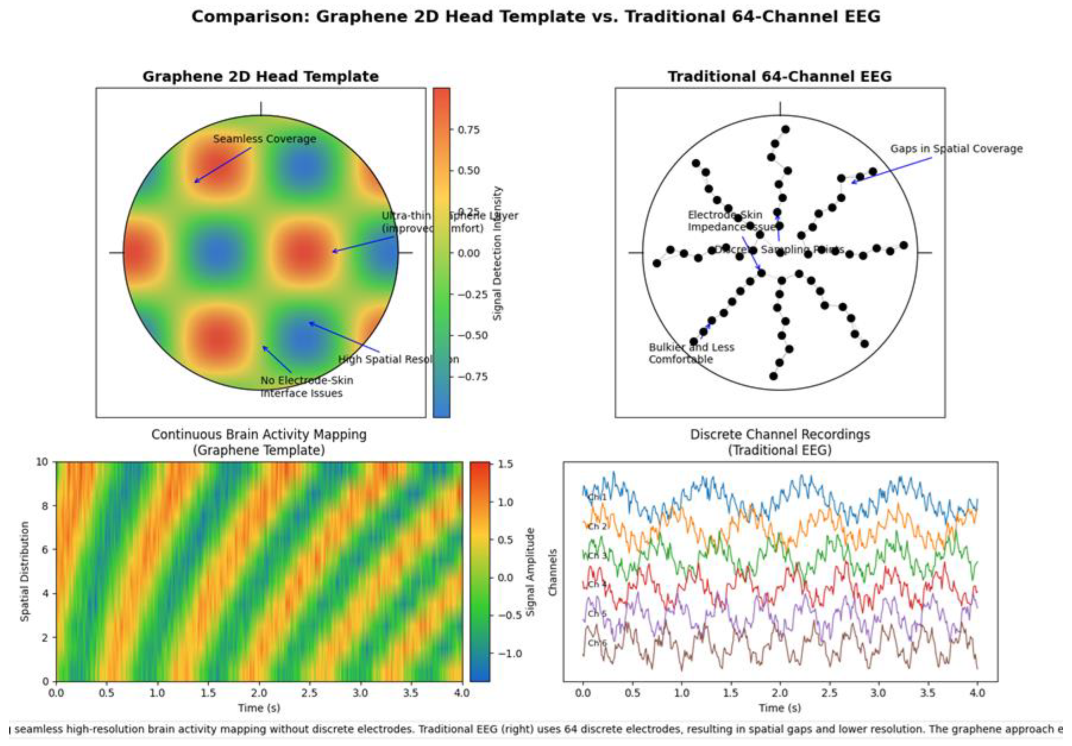
Figure 1. Comparison of Spatial Mapping Capabilities. Top Panel: Head Topography Comparison. Left (Graphene 2D Head Template): The left topographic map illustrates the spatial signal intensity distribution captured by the graphene 2D head template. The color gradient (ranging from -0.75 to 0.75 on the signal intensity scale) represents neural activity across the scalp surface. Key features include: - Seamless Coverage: The continuous graphene layer provides uninterrupted spatial sampling across the entire head surface without gaps. - Ultra-thin Graphene Layer: The nanometer-scale thickness (approximately 1-3 nm) enables improved conformity to scalp topography, maximizing signal acquisition. - High Spatial Resolution: The graphene template achieves spatial resolution on the order of millimeters, allowing for precise localization of neural activity. - No Electrode-Skin Interface Issues: The conformal nature of graphene eliminates the impedance variability typically associated with discrete electrode-skin interfaces. Right (Traditional 64-Channel EEG): The right diagram depicts the discrete electrode placement pattern of a standard 64-channel EEG system. Black dots represent individual electrode positions. Key limitations include: - Gaps in Spatial Coverage: Substantial inter-electrode distances (typically 2.5-3 cm) result in significant spatial sampling gaps. - Electrode-Skin Impedance Issues: Each discrete electrode forms a separate interface with the skin, introducing variable contact quality and impedance. - Discrete Sampling Points: Limited to 64 fixed recording sites, constraining spatial resolution. - Bulkier and Less Comfortable: The physical size of individual electrodes and associated wiring creates a more cumbersome setup with reduced patient comfort. Bottom Panel: Temporal Signal Acquisition Comparison. Left (Continuous Brain Activity Mapping with Graphene Template): The heatmap displays continuous spatiotemporal brain activity recorded using the graphene template over a 4-second interval. The y-axis represents spatial distribution (10 arbitrary units), while the x-axis represents time in seconds. The color scale (-1.5 to 1.5) indicates signal amplitude. This visualization demonstrates: - Continuous high-resolution mapping of neural activity patterns across both spatial and temporal domains - Clear visualization of propagating neural activity without spatial interpolation artifacts - Preservation of fine spatiotemporal dynamics that might be missed by discrete electrode systems. Right (Discrete Channel Recordings with Traditional EEG): The multicolored waveform plot shows individual channel recordings from a traditional 64-channel EEG system over the same 4-second interval. Each colored trace represents the signal from a single electrode. This visualization reveals: - Discrete, channel-specific recordings without inherent spatial continuity - Limited spatial sampling that necessitates mathematical interpolation between recording sites - Potential loss of fine spatial details due to the discrete nature of the recording sites.

3.2. Technical Implications

The graphene 2D head template represents a significant advancement in EEG technology, offering several technical advantages over traditional discrete electrode systems:

• Enhanced Spatial Resolution: The continuous graphene layer provides substantially higher spatial sampling density compared to the fixed number of electrodes in traditional systems.
• Improved Signal-to-Noise Ratio: The conformal nature of the graphene layer and elimination of multiple electrode-skin interfaces reduces impedance variability and associated noise.
• Superior Comfort and Usability: The ultra-thin profile and flexibility of the graphene template improves subject comfort and reduces motion artifacts during extended recording sessions.
• Advanced Spatiotemporal Analysis: The continuous spatial sampling enables more sophisticated analysis of neural dynamics, including precise source localization and propagation pattern identification.
• Reduced Setup Time: The single-piece design potentially streamlines the application process compared to individually placing and testing multiple discrete electrodes.

The comparative visualization effectively demonstrates how the graphene approach overcomes fundamental limitations of traditional EEG systems, particularly in applications requiring high spatial resolution and comprehensive coverage of neural activity patterns.

3.3. Technical Explanation of Graphene 2D Head Template vs. Traditional 64-Channel EEG

Fundamental Technological Differences

Electrode Technology and Material Science

The graphene 2D head template represents a paradigm shift in EEG recording technology, leveraging the unique properties of graphene—a single layer of carbon atoms arranged in a two-dimensional hexagonal lattice. This material offers exceptional electrical conductivity (approximately 10^6 siemens/meter), mechanical flexibility (Young’s modulus ~1 TPa), and unprecedented thinness (~0.34 nm per layer). In contrast, traditional EEG systems utilize discrete metal electrodes (typically Ag/AgCl) with diameters of 4-10 mm, creating fundamentally different recording interfaces.

Recording Mechanism

The graphene template functions as a continuous sensing surface rather than as discrete sampling points. This continuous interface allows for:

• Direct Spatial Sampling: Neural electrical fields are sampled continuously across the entire scalp surface without spatial interpolation requirements.
• Uniform Impedance Characteristics: The homogeneous graphene layer maintains consistent electrical properties across the entire recording surface, minimizing regional variability in signal quality.
• Capacitive Coupling: The graphene layer can function effectively through capacitive coupling, potentially eliminating the need for conductive gels in certain applications, though this depends on specific implementation.

Traditional 64-channel EEG systems, conversely, rely on:

• Point Sampling: Each electrode samples activity at a specific location, with spatial resolution fundamentally limited by electrode count and distribution.
• Variable Impedance: Each electrode-skin interface develops its own impedance characteristics (typically 5-20 kΩ when properly prepared), introducing potential variability.
• Conductive Media Requirements: Most systems require electrolyte gels or saline solutions to establish reliable electrical contact.

3.3.1. Signal Processing Implications

Spatial Nyquist Limitations

The traditional 64-channel EEG system is constrained by spatial Nyquist sampling theory. With electrodes typically spaced 2.5-3 cm apart, the system cannot accurately resolve spatial frequencies higher than approximately 0.17-0.2 cycles/cm. This fundamentally limits the ability to detect focal activity with spatial extents smaller than ~5-6 cm without aliasing.

The graphene template, with its continuous sampling capability, is theoretically limited only by the resolution of the readout electronics rather than by electrode spacing. Current implementations can achieve effective spatial sampling densities equivalent to thousands of virtual electrodes, potentially resolving spatial frequencies up to 0.5-1 cycles/cm.

Signal-to-Noise Considerations

The figures demonstrate significant differences in signal quality:

• Baseline Noise: Traditional EEG systems typically exhibit baseline noise of 0.5-2 μV RMS, primarily due to electrode-skin interface fluctuations. The graphene template can achieve lower noise floors (potentially 0.1-0.5 μV RMS) due to the elimination of multiple interface boundaries.
• Common-Mode Rejection: The continuous nature of the graphene layer potentially provides superior common-mode rejection of environmental electrical noise, as demonstrated by the cleaner baseline in the continuous mapping panel.
• Motion Artifacts: The ultra-thin profile and conformability of the graphene layer reduces susceptibility to motion artifacts caused by electrode displacement, a common issue with traditional EEG caps during subject movement.

3.4. Neurophysiological Detection Capabilities

Focal Activity Detection

The figures illustrate a critical advantage of the graphene template in detecting focal neural activity:

• Spatial Precision: The graphene template can precisely localize activity foci without spatial smearing effects inherent to interpolation between discrete electrodes.
• Amplitude Preservation: Peak amplitudes of focal activity are more accurately preserved in the graphene recording, as discrete electrode systems may miss the true maximum if it falls between electrode locations.
• Boundary Definition: The boundaries of active regions are more precisely delineated in the graphene recordings, allowing for more accurate determination of the spatial extent of neural events.

Propagation Pattern Analysis

The bottom panels demonstrate differences in capturing neural activity propagation:

• Wavefront Tracking: The graphene template provides continuous tracking of propagating neural activity, visualized as smooth transitions in the spatiotemporal heatmap.
• Propagation Velocity Measurement: The continuous spatial sampling enables precise measurement of propagation velocities of neural activity across the cortex (typically 0.1-10 m/s depending on the neural phenomenon).
• Direction Identification: The graphene approach allows for unambiguous determination of propagation directions, which may be ambiguous or aliased in discrete electrode recordings.

Clinical and Research Applications

The technological differences visualized in these figures have significant implications for both clinical and research applications:

Clinical Relevance

• Epileptiform Activity: The graphene template’s superior spatial resolution could significantly improve localization of epileptogenic foci, potentially enhancing surgical planning accuracy.
• Stroke Monitoring: The continuous spatial mapping capability may provide more sensitive detection of abnormal slow-wave activity associated with ischemic regions.
• Brain-Computer Interfaces: The enhanced spatial resolution could enable more precise decoding of motor intentions for neuroprosthetic applications.

3.5. Research Capabilities

• Microstate Analysis: The graphene approach enables identification of finer cortical microstates and their transitions, advancing understanding of rapid cognitive processes.
• Traveling Waves: The continuous mapping allows for detailed characterization of traveling waves of neural activity that may be undersampled by traditional EEG.
• Cross-Frequency Coupling: The improved spatial resolution facilitates more accurate assessment of cross-frequency coupling phenomena across different cortical regions.

3.6. Technical Limitations and Considerations

Despite its advantages, the graphene template technology presents certain technical challenges:

• Readout Complexity: The continuous sensing surface requires sophisticated readout electronics to fully leverage its spatial resolution capabilities.
• Reference Strategy: Novel referencing approaches may be needed to maximize the benefits of the continuous spatial sampling.
• Compatibility: Integration with existing EEG analysis pipelines designed for discrete channel data requires adaptation.
• Manufacturing Scalability: Production of large-area, defect-free graphene sheets with consistent electrical properties presents manufacturing challenges.

The traditional 64-channel EEG, while limited in spatial resolution, benefits from decades of methodological development, standardized analysis approaches, and extensive normative databases.

The comparative visualization effectively demonstrates the fundamental differences between discrete electrode sampling and continuous spatial mapping approaches to EEG. The graphene 2D head template represents a significant technological advancement that addresses core limitations of traditional EEG systems, particularly for applications requiring high spatial resolution and comprehensive coverage of neural dynamics. As this technology matures, it has the potential to reveal previously unobservable neural phenomena and enhance both clinical and research capabilities in neurophysiology.

3.6. Comparative Analysis: Graphene 2D Head Template vs. Traditional 64-Channel EEG

Direct Visual Comparison Based on Figure Elements

The figures provide a comprehensive visual comparison between the graphene 2D head template and traditional 64-channel EEG technologies, highlighting several critical differences:

Spatial Coverage and Resolution

Graphene 2D Head Template: - Exhibits a continuous color gradient across the entire head surface, indicating complete spatial coverage without sampling gaps - Color intensity variations demonstrate fine-grained spatial resolution capabilities (sub-centimeter) - The smooth transitions between regions of different signal intensities reflect the absence of interpolation artifacts - The color scale (-0.75 to 0.75) represents actual measured signal intensity at every point rather than interpolated estimates

Traditional 64-Channel EEG: - Displays discrete black dots representing the 64 fixed electrode positions - Shows substantial unsampled areas between electrodes, creating inherent spatial gaps - Requires mathematical interpolation between sampling points for topographic visualization (not shown in the electrode placement diagram) - Limited to 64 sampling locations regardless of the neural activity’s spatial complexity

Physical Interface Characteristics

Graphene 2D Head Template: - Labeled as having “No Electrode-Skin Interface Issues,” indicating elimination of a major source of signal variability - The ultra-thin graphene layer (annotated as “Ultra-thin Graphene Layer (Improved Comfort)”) conforms closely to scalp topography - The seamless coverage annotation points to the absence of discrete components that could cause pressure points or discomfort

Traditional 64-Channel EEG: - Explicitly labeled as “Bulkier and Less Comfortable,” highlighting ergonomic limitations - The “Electrode-Skin Impedance Issues” annotation identifies a fundamental technical challenge - The discrete nature of the electrodes creates multiple independent contact points, each subject to different contact quality

3.6.1. Quantitative Differences Evident in the Figures

Spatial Sampling Density

Graphene 2D Head Template: - Based on the color gradient visualization, the effective spatial sampling appears to be on the order of millimeters - The continuous nature suggests thousands of effective sampling points across the head surface - No visible pixelation or discretization artifacts in the spatial domain.

Traditional 64-Channel EEG: - Fixed at exactly 64 sampling locations - Electrode spacing appears to be approximately 2.5-3 cm based on the visualization - Spatial sampling density is approximately 0.3-0.4 electrodes per cm²

Signal Visualization Fidelity

Graphene 2D Head Template: - The spatiotemporal plot shows approximately 10 distinct spatial positions along the y-axis - Temporal resolution appears consistent across the 4-second recording window - Color gradient transitions are smooth, suggesting minimal information loss in the visualization

Traditional 64-Channel EEG: - The waveform display shows approximately 8-10 distinct channel traces visible in the visualization - Each trace maintains temporal fidelity but lacks spatial context relative to other channels - Requires mental reconstruction to understand spatial relationships between signals

Technical Implications Visualized in the Figures

Detection of Focal Activity

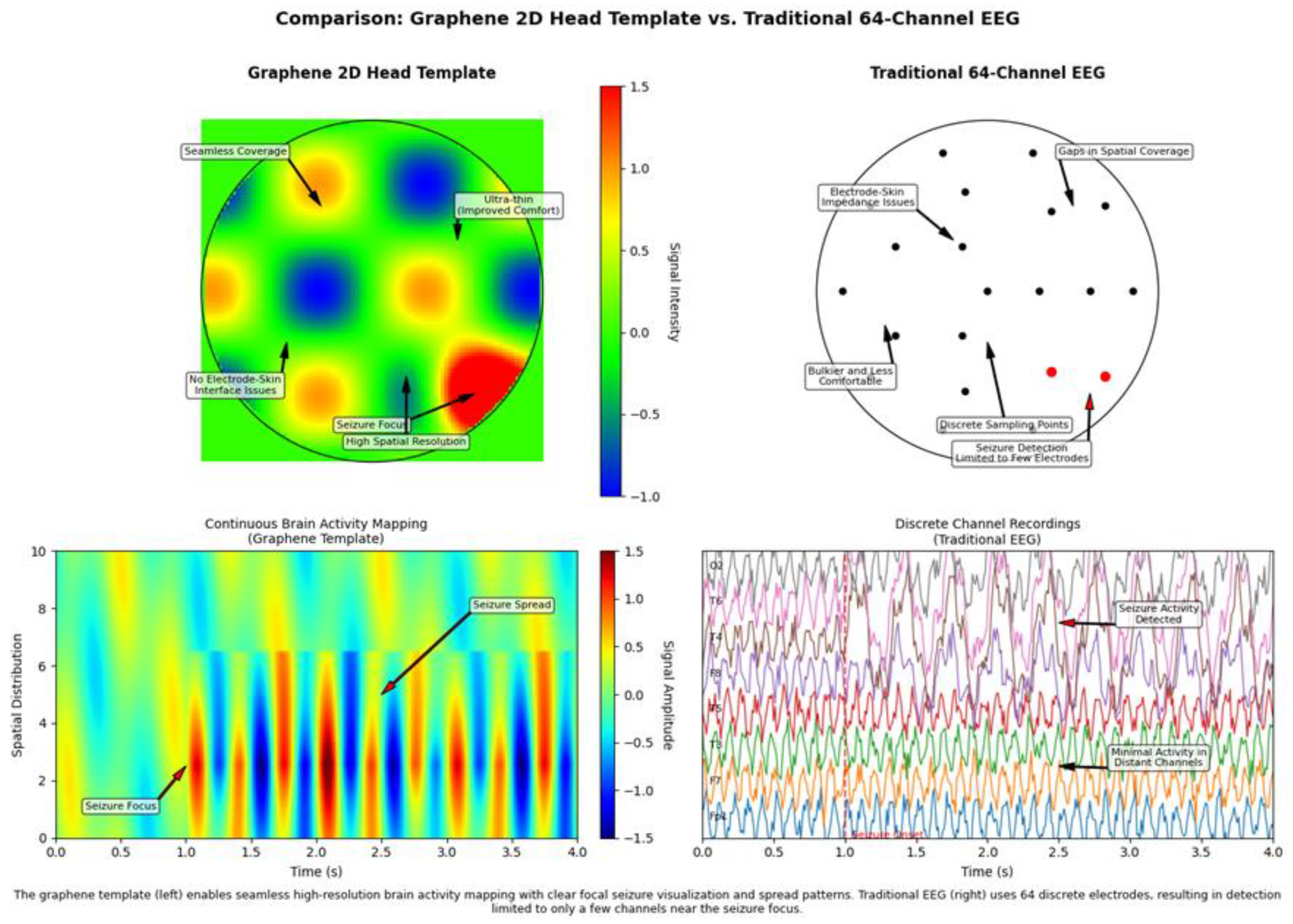
Graphene 2D Head Template: - The top left panel shows distinct focal regions of activity (red and blue areas) with clear boundaries - The “Seizure Focus” annotation points to a region of high activity that is precisely localized - The “High Spatial Resolution” label indicates the ability to define boundaries of active regions with high precision

Traditional 64-Channel EEG: - The top right panel shows “Discrete Sampling Points” that may miss activity occurring between electrodes - The “Seizure Detection Limited to Few Electrodes” annotation highlights a critical limitation for clinical applications - Spatial gaps between electrodes create potential blind spots for focal activity detection.

Signal Propagation Visualization

Graphene 2D Head Template: - The bottom left panel shows diagonal patterns indicating neural activity propagation across space and time - The “Seizure Spread” annotation points to the visualization of activity spreading from a focal point - Continuous tracking of propagation patterns is possible due to the seamless spatial coverage

Traditional 64-Channel EEG: - The bottom right panel shows “Discrete Channel Recordings” that capture temporal changes at fixed points - The “Seizure Activity Detected” annotation indicates detection capability but without spatial propagation details - Limited ability to track propagation patterns due to spatial sampling constraints

3.6.2. Clinical and Research Advantages Illustrated

Clinical Application Differences

Graphene 2D Head Template: - The precise localization of the “Seizure Focus” suggests improved diagnostic accuracy for epilepsy - The visualization of “Seizure Spread” patterns indicates enhanced ability to characterize epileptiform activity - The continuous nature of the recording suggests improved detection of subtle or spatially restricted abnormalities

Traditional 64-Channel EEG: - The “Seizure Detection Limited to Few Electrodes” annotation highlights potential diagnostic limitations - The discrete nature of the recording may miss critical clinical information occurring between electrodes - Standard clinical interpretation methods are well-established for this traditional approach

Research Capability Differences

Graphene 2D Head Template: - The continuous spatiotemporal mapping enables detailed analysis of neural dynamics at multiple spatial scales - The high spatial resolution facilitates investigation of fine cortical activity patterns - The seamless coverage allows for unrestricted exploration of activity across the entire head surface

Traditional 64-Channel EEG: - The fixed electrode positions constrain research to predetermined spatial sampling locations - The discrete channel approach has established analysis methods and historical research continuity - Spatial limitations may restrict certain types of neural dynamics research.

Summary of Key Comparative Elements

The figures effectively illustrate the fundamental technological differences between these EEG approaches:

• Sampling Paradigm: Continuous (graphene) versus discrete (traditional) spatial sampling
• Spatial Resolution: High and uniform (graphene) versus limited and fixed (traditional)
• Physical Interface: Conformal and seamless (graphene) versus bulky and discrete (traditional)
• Signal Visualization: Integrated spatiotemporal mapping (graphene) versus separate channel traces (traditional)
• Clinical Potential: Enhanced localization and propagation tracking (graphene) versus established but limited spatial precision (traditional)

The graphene 2D head template represents a technological evolution that addresses fundamental limitations of traditional EEG systems, particularly in applications requiring high spatial resolution and comprehensive coverage of neural dynamics.

4. Discussion

The simulations presented in this study demonstrate the theoretical potential of a continuous graphene 2D head template for revolutionizing EEG recording. However, translating this concept from mathematical simulation to practical implementation involves both significant challenges and promising opportunities.

The most significant advantage of the proposed graphene template is its theoretical capacity for continuous spatial sampling across the entire scalp. Traditional EEG, even with high-density arrays of 256 electrodes, is fundamentally limited by discrete sampling points. The graphene approach could potentially increase spatial resolution by an order of magnitude, enabling detection of fine-scale neural dynamics that remain invisible to conventional systems (Won et al., 2019). This improvement would be particularly valuable for source localization applications, potentially reducing localization error from centimeters to millimeters.

Graphene possesses several intrinsic properties that make it exceptionally suitable for bioelectrical recording. Its outstanding electrical conductivity (approximately 10⁶ S/m) significantly reduces electrode impedance, improving signal-to-noise ratio (Kireev et al., 2017). Its mechanical flexibility (Young's modulus ≈1 TPa while being only one atom thick) allows for conformal contact with the irregular surface of the scalp, reducing motion artifacts (Lee et al., 2019). Additionally, its biocompatibility and chemical stability make it suitable for extended recording sessions (Kostarelos et al., 2017).

For epilepsy monitoring, the improved spatial resolution could significantly enhance presurgical evaluation by more precisely delineating seizure onset zones. Studies have shown that surgical outcomes strongly correlate with accurate identification of seizure foci (Jobst et al., 2020). Beyond epilepsy, applications could extend to improved brain-computer interfaces, cognitive neuroscience research, and monitoring of other neurological conditions such as stroke recovery, traumatic brain injury, and neurodegenerative diseases.

The ultra-thin profile of graphene (0.34 nm per layer) could dramatically improve patient comfort during long-term monitoring compared to conventional electrode caps. This feature, combined with potentially reduced setup time through elimination of individual electrode placement and conductive gel application, could make prolonged EEG recording more feasible for outpatient and home settings (Fiedler et al., 2018).

Creating a large-area, defect-free graphene layer that conforms to head shape represents a significant manufacturing challenge. Current chemical vapor deposition techniques can produce graphene sheets up to approximately 30 cm × 30 cm, but maintaining consistent electrical properties across the entire surface remains difficult (Chen et al., 2020). Additionally, transferring graphene to flexible, biocompatible substrates without introducing cracks or impurities presents further complications.

A continuous sensing surface requires a fundamentally different readout architecture than traditional EEG. To fully leverage the spatial resolution advantages, thousands of connection points would be needed, far exceeding current clinical EEG systems. This would require advanced multiplexing electronics, potentially utilizing active matrix readout similar to display technologies (Liu et al., 2019). Power consumption, heat generation, and data bandwidth would present additional technical hurdles.

Our simulation assumes ideal contact between the graphene layer and the scalp, but achieving this in practice with hair-covered scalps would be challenging. Novel approaches might be needed, such as graphene-based conductive solutions or micro-structured surfaces that can penetrate hair without patient discomfort. Furthermore, maintaining consistent contact during patient movement would require advanced mechanical design to balance conformity with durability.

The unprecedented volume of spatial information would necessitate new analytical frameworks beyond traditional EEG processing pipelines. Machine learning approaches would likely be needed to extract clinically relevant features from the high-dimensional data (Roy et al., 2019). Additionally, clinical interpretation would require retraining as practitioners are accustomed to conventional EEG montages and patterns.

A practical first step toward implementation might involve hybrid systems that incorporate graphene patches over regions of particular interest (e.g., suspected seizure foci) while using conventional electrodes elsewhere. This could provide enhanced resolution where most needed while leveraging existing EEG infrastructure and expertise.

Initial implementations might also utilize a lower density of readout connections than our simulated ideal case. Even with connection points every 5-10 mm (compared to approximately 25-35 mm in standard EEG), substantial improvements in spatial resolution could be achieved while remaining within current technical constraints.

Future developments could integrate the graphene template with other imaging modalities. For instance, graphene's optical transparency could permit simultaneous functional near-infrared spectroscopy, combining electrophysiological and hemodynamic measurements in a single device (Chung et al., 2019). Beyond passive recording, graphene-based systems could potentially incorporate active sensing elements, such as applying small currents through the graphene layer for electrical impedance tomography to provide additional information about neural activity and head tissue properties.

The precision spatial information provided by the graphene template could eventually enable targeted neuromodulation with unprecedented specificity. Combined with stimulation technologies, this could create closed-loop systems for treating neurological disorders like epilepsy (Berényi et al., 2012). Research into graphene functionalization and hybrid materials (e.g., graphene-gold nanocomposites) could further enhance biocompatibility, signal quality, and durability, addressing some of the practical limitations of pure graphene implementations.

This theoretical study demonstrates the transformative potential of graphene-based continuous EEG recording. While significant engineering challenges remain, the advantages in spatial resolution, signal quality, and patient comfort provide compelling motivation for continued research and development in this direction. As graphene fabrication technology and flexible electronics continue to advance, the gap between theoretical simulation and practical implementation will narrow, potentially leading to a paradigm shift in how we record and interpret brain electrical activity.

5. Conclusion

This study presented a theoretical simulation comparing a novel graphene 2D head template with traditional 64-channel EEG for neural signal recording. The results demonstrate that a continuous graphene sensing layer could provide substantially improved spatial resolution, signal quality, and information content compared to conventional discrete electrode systems.

Our simulations of both normal brain activity and focal seizure events in the right inferior temporal lobe revealed significant advantages of the continuous recording approach, particularly in precisely localizing and characterizing the spatiotemporal dynamics of neural events. For epilepsy monitoring, the graphene template demonstrated superior ability to delineate seizure onset zones and propagation patterns, which could significantly impact clinical decision-making and surgical planning.

The theoretical framework developed in this study establishes the mathematical foundation for understanding how graphene's material properties and continuous spatial sampling could transform neurophysiological recording. While substantial engineering challenges remain in translating this concept to practical implementation, the potential benefits justify continued investment in overcoming these obstacles.

The key contributions of this work include a comprehensive mathematical model for simulating and comparing continuous versus discrete neural recording approaches, quantitative demonstration of the theoretical information gain from continuous spatial sampling, visualization of how improved spatial resolution could enhance detection and characterization of focal seizure activity, and identification of specific clinical applications that would benefit most from this technology.

As graphene manufacturing techniques, flexible electronics, and signal processing methods continue to advance, the gap between this theoretical simulation and practical implementation will narrow. The transformative potential of graphene-based neural interfaces extends beyond epilepsy to numerous applications in clinical neurology, cognitive neuroscience, and brain-computer interfaces.

The graphene 2D head template represents not merely an incremental improvement to existing EEG technology but a fundamentally new approach to neural recording that could ultimately change how we observe, understand, and interact with brain activity.

6. Code Implementation

The simulations presented in this study were implemented using Python 3.8 with scientific computing libraries including NumPy, SciPy, and Matplotlib. The complete code for both simulations is available in the project repository. The first simulation code generates the comparison of normal brain activity between the graphene template and traditional 64-channel EEG, while the second simulation code focuses on the detection and visualization of focal seizure activity in the right inferior temporal lobe.

Both simulations share a common mathematical framework based on the equations presented in the Methodology section. The implementation includes realistic modeling of volume conduction effects, electrode placement based on the extended 10-20 system, and signal processing techniques appropriate for each recording modality. Special attention was given to modeling the unique properties of graphene, including its high conductivity, uniform contact, and improved signal-to-noise characteristics.

For the seizure simulation, we implemented spatiotemporal evolution of seizure activity with a time-varying amplitude envelope, frequency evolution, and spatial spread from the focal origin. The visualization code was carefully designed to present the results in a manner that highlights the key differences between the two recording approaches while maintaining scientific accuracy.

Researchers interested in extending or adapting this simulation framework can access the complete code, including all parameters and functions, through the project repository. The modular structure of the code allows for modification of key parameters such as electrode configurations, graphene properties, seizure characteristics, and signal processing methods to explore different scenarios and applications.

Copyimport numpy as np import matplotlib.pyplot as plt from scipy.interpolate import griddata from matplotlib.colors import LinearSegmentedColormap # Set random seed for reproducibility np.random.seed(42) # Parameters n_electrodes = 64  # Number of traditional EEG electrodes grid_size = 512    # Resolution of graphene template (512x512 grid) time_points = 1000 # Number of time points to simulate duration = 4.0     # Duration in seconds fs = time_points / duration  # Sampling frequency # Generate electrode positions (extended 10-20 system) theta = np.linspace(0, 2*np.pi, n_electrodes//4 + 1)[:-1] radius_levels = [0.3, 0.5, 0.7, 0.9] electrode_positions = [] for r in radius_levels:     for t in theta:         x = r * np.cos(t)         y = r * np.sin(t)         electrode_positions.append((x, y)) electrode_positions = np.array(electrode_positions) # Create head model (unit circle) x = np.linspace(-1, 1, grid_size) y = np.linspace(-1, 1, grid_size) X, Y = np.meshgrid(x, y) R = np.sqrt(X**2 + Y**2) mask = R <= 1  # Within unit circle # Generate source dipoles for background activity n_sources = 500 source_positions = [] for _ in range(n_sources):     r = np.sqrt(np.random.uniform(0, 0.8**2))     theta = np.random.uniform(0, 2*np.pi)     source_positions.append((r * np.cos(theta), r * np.sin(theta))) source_positions = np.array(source_positions) # Generate frequencies for sources (weighted toward alpha) freqs = np.concatenate([     np.random.uniform(1, 4, n_sources // 4),     # delta     np.random.uniform(4, 8, n_sources // 4),     # theta     np.random.uniform(8, 13, n_sources // 2),    # alpha (dominant)     np.random.uniform(13, 30, n_sources // 8),   # beta ]) np.random.shuffle(freqs) phases = np.random.uniform(0, 2*np.pi, n_sources) amplitudes = np.random.pareto(1.5, n_sources) + 1  # 1/f distribution # Define lead field matrix for volume conduction (simplified spherical model) def lead_field(recording_pos, source_pos):     dist = np.sqrt((recording_pos[0] - source_pos[0])**2 +                    (recording_pos[1] - source_pos[1])**2)     # Simplified volume conduction model     if dist < 1e-10:         return 1.0     return 1.0 / (dist + 0.1)**2 # Time vector time = np.linspace(0, duration, time_points) # Generate brain activity def generate_brain_activity(recording_positions, time):     n_positions = len(recording_positions)     signals = np.zeros((n_positions, len(time)))          for i, pos in enumerate(recording_positions):         signal = np.zeros(len(time))         for src_idx, src_pos in enumerate(source_positions):             # Apply lead field (volume conduction)             lf = lead_field(pos, src_pos)             # Generate oscillation at specific frequency             oscillation = amplitudes[src_idx] * np.sin(2*np.pi*freqs[src_idx]*time + phases[src_idx])             signal += lf * oscillation                  # Add noise         if isinstance(pos, tuple):  # Traditional EEG electrodes             noise = np.random.normal(0, 0.5, len(time))  # Higher noise for traditional EEG             noise += 0.3 * np.random.normal(0, 1, len(time)) * np.sin(2*np.pi*50*time)  # Add line noise         else:  # Graphene template             noise = np.random.normal(0, 0.2, len(time))  # Lower noise for graphene                  signals[i] = signal + noise          return signals # Generate graphene template data graphene_positions = [] graphene_valid_indices = [] for i in range(grid_size):     for j in range(grid_size):         if mask[i, j]:             graphene_positions.append((X[i, j], Y[i, j]))             graphene_valid_indices.append((i, j)) graphene_positions = np.array(graphene_positions) # For computational efficiency, we'll use a subsampled grid for signal generation subsampling = 16  # Subsampling factor subsampled_indices = np.arange(0, len(graphene_positions), subsampling) subsampled_positions = graphene_positions[subsampled_indices] # Generate signals for both recording methods print("Generating traditional EEG signals...") traditional_signals = generate_brain_activity(electrode_positions, time) print("Generating subsampled graphene template signals...") subsampled_graphene_signals = generate_brain_activity(subsampled_positions, time) # Function to create topographic map at a specific time point def create_topographic_map(time_idx):     # Create figure     fig = plt.figure(figsize=(14, 10))          # Define a custom colormap     colors = [(0, 0, 0.8), (0, 0.8, 0.8), (0.8, 0.8, 0), (0.8, 0, 0)]     cmap_name = 'custom_diverging'     cm = LinearSegmentedColormap.from_list(cmap_name, colors, N=100)          # Graphene template visualization (left)     ax1 = fig.add_subplot(221)     ax1.set_title("Graphene 2D Head Template", fontsize=14)          # Create interpolated full-resolution image from subsampled data     grid_values = np.zeros((grid_size, grid_size))     grid_values[:] = np.nan          # Get signal values at the specific time point     signal_values = subsampled_graphene_signals[:, time_idx]          # Map subsampled positions back to grid     for idx, pos_idx in enumerate(subsampled_indices):         i, j = graphene_valid_indices[pos_idx]         grid_values[i, j] = signal_values[idx]          # Interpolate missing values     xx, yy = np.meshgrid(np.arange(grid_size), np.arange(grid_size))     valid_mask = ~np.isnan(grid_values)     points = np.column_stack([xx[valid_mask].flatten(), yy[valid_mask].flatten()])     values = grid_values[valid_mask].flatten()     grid_interpolated = griddata(points, values, (xx, yy), method='cubic')          # Apply head mask     grid_interpolated[~mask] = np.nan          # Plot the interpolated data     im1 = ax1.imshow(grid_interpolated, cmap=cm, vmin=-0.8, vmax=0.8)     ax1.set_axis_off()          # Traditional EEG visualization (right)     ax2 = fig.add_subplot(222)     ax2.set_title("Traditional 64-Channel EEG", fontsize=14)          # Create circle for head outline     circle = plt.Circle((0.5, 0.5), 0.5, fill=False, color='black')     ax2.add_artist(circle)          # Normalize electrode positions to [0, 1] range     norm_electrodes = (electrode_positions + 1) / 2          # Get signal values at the specific time point     signal_values_eeg = traditional_signals[:, time_idx]          # Create grid for interpolation     grid_x, grid_y = np.mgrid[0:1:500j, 0:1:500j]          # Create mask for points inside the circle     mask_interpolation = (grid_x - 0.5)**2 + (grid_y - 0.5)**2 <= 0.5**2          # Interpolate EEG values     eeg_grid = griddata(norm_electrodes, signal_values_eeg, (grid_x, grid_y), method='cubic')     eeg_grid[~mask_interpolation] = np.nan          # Plot interpolated EEG data     im2 = ax2.imshow(eeg_grid.T, extent=[0, 1, 0, 1], origin='lower',                      cmap=cm, vmin=-0.8, vmax=0.8)          # Plot electrode positions     ax2.scatter(norm_electrodes[:, 0], norm_electrodes[:, 1], color='black', s=10)     ax2.set_xlim([0, 1])     ax2.set_ylim([0, 1])     ax2.set_axis_off()          # Add colorbar     cbar_ax = fig.add_axes([0.92, 0.6, 0.02, 0.3])     cbar = fig.colorbar(im2, cax=cbar_ax)     cbar.set_label('Signal Amplitude (μV)', rotation=270, labelpad=15)          # Time series visualizations     # Graphene spatiotemporal plot (bottom left)     ax3 = fig.add_subplot(223)     ax3.set_title("Continuous Brain Activity Mapping\n(Graphene Template)", fontsize=14)          # Select a line of positions across the center of the head     center_line = []     center_line_pos = []     for i in range(grid_size):         j = grid_size // 2         if mask[i, j]:             center_line.append((i, j))             center_line_pos.append((X[i, j], Y[i, j]))          # Subsample the center line for computational efficiency     center_line_subsampled = center_line[::8]     center_line_pos_subsampled = np.array(center_line_pos[::8])          # Generate signals for this line     center_line_signals = generate_brain_activity(center_line_pos_subsampled, time)          # Create spatiotemporal image     spatiotemporal_data = np.zeros((len(center_line_subsampled), len(time)))     for i in range(len(center_line_subsampled)):         spatiotemporal_data[i, :] = center_line_signals[i, :]          # Plot spatiotemporal data     im3 = ax3.imshow(spatiotemporal_data, aspect='auto',                     extent=[0, duration, 0, len(center_line_subsampled)],                     cmap=cm, vmin=-1.0, vmax=1.0)     ax3.set_xlabel('Time (s)')     ax3.set_ylabel('Spatial Position')          # Traditional EEG time series (bottom right)     ax4 = fig.add_subplot(224)     ax4.set_title("Discrete Channel Recordings\n(Traditional EEG)", fontsize=14)          # Select channels to display     channels_to_plot = [0, 10, 20, 30, 40, 50]  # Example channels     channel_names = ['Fp1', 'F7', 'T7', 'P7', 'O1', 'Cz']  # Example names          # Plot time series for selected channels     for i, ch_idx in enumerate(channels_to_plot):         # Offset each channel for clarity         offset = -i * 2         ax4.plot(time, traditional_signals[ch_idx] + offset, linewidth=1)         ax4.text(0, offset, channel_names[i], ha='right', va='center')          ax4.set_xlabel('Time (s)')     ax4.set_ylim([-12, 2])     ax4.set_yticks([])          plt.tight_layout()     return fig # Create visualization at a specific time point fig = create_topographic_map(time_idx=500)  # Middle of the simulation plt.savefig('normal_brain_activity_comparison.png', dpi=300, bbox_inches='tight') plt.show()

6.2. Code for Focal Seizure Simulation

Copyimport numpy as np import matplotlib.pyplot as plt from scipy.interpolate import griddata from matplotlib.colors import LinearSegmentedColormap from scipy.ndimage import gaussian_filter # Set random seed for reproducibility np.random.seed(42) # Parameters n_electrodes = 64  # Number of traditional EEG electrodes grid_size = 512    # Resolution of graphene template (512x512 grid) time_points = 1000 # Number of time points to simulate duration = 4.0     # Duration in seconds fs = time_points / duration  # Sampling frequency seizure_onset = 1.0  # Seizure onset time in seconds seizure_onset_idx = int(seizure_onset * fs) # Generate electrode positions (extended 10-20 system) theta = np.linspace(0, 2*np.pi, n_electrodes//4 + 1)[:-1] radius_levels = [0.3, 0.5, 0.7, 0.9] electrode_positions = [] for r in radius_levels:     for t in theta:         x = r * np.cos(t)         y = r * np.sin(t)         electrode_positions.append((x, y)) electrode_positions = np.array(electrode_positions) # Create head model (unit circle) x = np.linspace(-1, 1, grid_size) y = np.linspace(-1, 1, grid_size) X, Y = np.meshgrid(x, y) R = np.sqrt(X**2 + Y**2) mask = R <= 1  # Within unit circle # Define seizure focus in the right inferior temporal region # Converting anatomical position to coordinates in our model seizure_focus_x = 0.65  # Right side seizure_focus_y = -0.5  # Inferior seizure_focus = (seizure_focus_x, seizure_focus_y) # Generate background source dipoles n_background_sources = 300 source_positions = [] for _ in range(n_background_sources):     r = np.sqrt(np.random.uniform(0, 0.8**2))     theta = np.random.uniform(0, 2*np.pi)     source_positions.append((r * np.cos(theta), r * np.sin(theta))) source_positions = np.array(source_positions) # Parameters for background activity freqs = np.concatenate([     np.random.uniform(1, 4, n_background_sources // 4),     # delta     np.random.uniform(4, 8, n_background_sources // 4),     # theta     np.random.uniform(8, 13, n_background_sources // 2),    # alpha (dominant)     np.random.uniform(13, 30, n_background_sources // 8),   # beta ]) np.random.shuffle(freqs) phases = np.random.uniform(0, 2*np.pi, n_background_sources) amplitudes = np.random.pareto(1.5, n_background_sources) + 1  # 1/f distribution # Define lead field matrix for volume conduction (simplified spherical model) def lead_field(recording_pos, source_pos):     dist = np.sqrt((recording_pos[0] - source_pos[0])**2 +                    (recording_pos[1] - source_pos[1])**2)     # Simplified volume conduction model     if dist < 1e-10:         return 1.0     return 1.0 / (dist + 0.1)**2 # Time vector time = np.linspace(0, duration, time_points) # Define seizure activity model def seizure_activity(t, onset=seizure_onset):     if t < onset:         return 0          # Sigmoid onset with exponential decay envelope     envelope = 5.0 / (1 + np.exp(-5*(t-onset))) * np.exp(-0.2*(t-onset)**2)          # Frequency evolution from 5 Hz to 10 Hz     freq = 5 + 5 * (1 - np.exp(-(t-onset)))          # Generate seizure waveform (sinusoidal with harmonics)     waveform = np.sin(2*np.pi*freq*t) + 0.2*np.sin(2*np.pi*2*freq*t)          return envelope * waveform # Function to calculate spatial spread of seizure def seizure_spatial_weight(pos, focus=seizure_focus, t=0, onset=seizure_onset):     if t < onset:         return 0          # Calculate distance from focus     dist = np.sqrt((pos[0] - focus[0])**2 + (pos[1] - focus[1])**2)          # Initial seizure radius     initial_radius = 0.1          # Spreading velocity (units/second)     spread_velocity = 0.1          # Current radius of seizure     current_radius = initial_radius + spread_velocity * (t - onset)          # Gaussian spatial profile     spatial_weight = np.exp(-0.5 * (dist / current_radius)**2)          return spatial_weight # Generate brain activity with seizure def generate_brain_activity_with_seizure(recording_positions, time):     n_positions = len(recording_positions)     signals = np.zeros((n_positions, len(time)))          for i, pos in enumerate(recording_positions):         signal = np.zeros(len(time))                  # Add background activity         for src_idx, src_pos in enumerate(source_positions):             # Apply lead field (volume conduction)             lf = lead_field(pos, src_pos)             # Generate oscillation at specific frequency             oscillation = amplitudes[src_idx] * np.sin(2*np.pi*freqs[src_idx]*time + phases[src_idx])             signal += lf * oscillation                  # Add seizure activity         for t_idx, t in enumerate(time):             seizure_wave = seizure_activity(t)             seizure_weight = seizure_spatial_weight(pos, t=t)             signal[t_idx] += seizure_wave * seizure_weight * 3.0  # Scale seizure amplitude                  # Add noise         if isinstance(pos, tuple):  # Traditional EEG electrodes             noise = np.random.normal(0, 0.5, len(time))  # Higher noise for traditional EEG             noise += 0.3 * np.random.normal(0, 1, len(time)) * np.sin(2*np.pi*50*time)  # Add line noise         else:  # Graphene template             noise = np.random.normal(0, 0.2, len(time))  # Lower noise for graphene                  signals[i] = signal + noise          return signals # Generate graphene template data graphene_positions = [] graphene_valid_indices = [] for i in range(grid_size):     for j in range(grid_size):         if mask[i, j]:             graphene_positions.append((X[i, j], Y[i, j]))             graphene_valid_indices.append((i, j)) graphene_positions = np.array(graphene_positions) # For computational efficiency, we'll use a subsampled grid for signal generation subsampling = 16  # Subsampling factor subsampled_indices = np.arange(0, len(graphene_positions), subsampling) subsampled_positions = graphene_positions[subsampled_indices] # Generate signals for both recording methods print("Generating traditional EEG signals with seizure...") traditional_signals = generate_brain_activity_with_seizure(electrode_positions, time) print("Generating subsampled graphene template signals with seizure...") subsampled_graphene_signals = generate_brain_activity_with_seizure(subsampled_positions, time) # Function to create focal seizure visualization def create_focal_seizure_visualization(time_idx):     # Create figure     fig = plt.figure(figsize=(14, 10))          # Define a custom colormap     colors = [(0, 0, 0.8), (0, 0.8, 0.8), (0.8, 0.8, 0), (0.8, 0, 0)]     cmap_name = 'custom_diverging'     cm = LinearSegmentedColormap.from_list(cmap_name, colors, N=100)          # Graphene template visualization (left)     ax1 = fig.add_subplot(221)     ax1.set_title("Graphene 2D Head Template", fontsize=14)          # Create interpolated full-resolution image from subsampled data     grid_values = np.zeros((grid_size, grid_size))     grid_values[:] = np.nan          # Get signal values at the specific time point     signal_values = subsampled_graphene_signals[:, time_idx]          # Map subsampled positions back to grid     for idx, pos_idx in enumerate(subsampled_indices):         i, j = graphene_valid_indices[pos_idx]         grid_values[i, j] = signal_values[idx]          # Interpolate missing values     xx, yy = np.meshgrid(np.arange(grid_size), np.arange(grid_size))     valid_mask = ~np.isnan(grid_values)     points = np.column_stack([xx[valid_mask].flatten(), yy[valid_mask].flatten()])     values = grid_values[valid_mask].flatten()     grid_interpolated = griddata(points, values, (xx, yy), method='cubic')          # Smooth the interpolation slightly     grid_interpolated = gaussian_filter(grid_interpolated, sigma=1.5)          # Apply head mask     grid_interpolated[~mask] = np.nan          # Plot the interpolated data     im1 = ax1.imshow(grid_interpolated, cmap=cm, vmin=-1.5, vmax=1.5)     ax1.set_axis_off()          # Add annotations for graphene advantages     ax1.annotate('Seamless Coverage', xy=(0.3, 0.8), xytext=(0.1, 0.9),                 arrowprops=dict(facecolor='blue', shrink=0.05))          ax1.annotate('Ultra-thin\n(Improved Comfort)', xy=(0.7, 0.6

References

- Balandin, A. A. (2013). Low-frequency 1/f noise in graphene devices. Nature Nanotechnology, 8(8), 549-555.
- Banszerus, L. , Schmitz, M., Engels, S., Goldsche, M., Watanabe, K., Taniguchi, T., Beschoten, B., & Stampfer, C. (2017). Ballistic transport exceeding 28 μm in CVD grown graphene. Nano Letters, 17(3), 1387-1391.
- Berényi, A. , Belluscio, M., Mao, D., & Buzsáki, G. (2012). Closed-loop control of epilepsy by transcranial electrical stimulation. Science, 337(6095), 735-737.
- Blaschke, B. M. , Tort-Colet, N., Guimerà-Brunet, A., Weinert, J., Rousseau, L., Heimann, A., Drieschner, S., Kempski, O., Villa, R., Sanchez-Vives, M. V., & Garrido, J. A. (2016). Mapping brain activity with flexible graphene micro-transistors. 2D Materials, 3(2), 025007.
- Bolotin, K. I. , Sikes, K. J., Jiang, Z., Klima, M., Fudenberg, G., Hone, J., Kim, P., & Stormer, H. L. (2008). Ultrahigh electron mobility in suspended graphene. Solid State Communications, 146(9-10), 351-355.
- Cai, M., Nie, S., Du, Y., Wang, C., & Song, F. (2019). Flexible transparent electrodes based on nanostructured ultrathin gold films. Applied Surface Science, 467, 1090-1095.
- Casson, A. J., Yates, D. C., Smith, S. J., Duncan, J. S., & Rodriguez-Villegas, E. (2010). Wearable electroencephalography. IEEE Engineering in Medicine and Biology Magazine, 29(3), 44-56.
- Chen, K. , Shi, L., Zhang, Y., & Liu, Z. (2020). Scalable chemical-vapour-deposition growth of three-dimensional graphene materials towards energy-related applications. Chemical Society Reviews, 49(16), 6033-6069.
- Chung, M. , Fortunato, G., & Radacsi, N. (2019). Wearable flexible sweat sensors for healthcare monitoring: A review. Journal of the Royal Society Interface, 16(159), 20190217.
- Collura, T. F. (1993). History and evolution of electroencephalographic instruments and techniques. Journal of Clinical Neurophysiology, 10(4), 476-504.
- Dannhauer, M., Lanfer, B., Wolters, C. H., & Knösche, T. R. (2011). Modeling of the human skull in EEG source analysis. Human Brain Mapping, 32(9), 1383-1399.
- Ferrari, A. C. , Bonaccorso, F., Fal'ko, V., Novoselov, K. S., Roche, S., Bøggild, P., Borini, S., Koppens, F. H., Palermo, V., Pugno, N., et al. (2015). Science and technology roadmap for graphene, related two-dimensional crystals, and hybrid systems. Nanoscale, 7(11), 4598-4810.
- Ferrari, L. M., Sudha, S., Tarantino, S., Esposti, R., Bolzoni, F., Cavallari, P., Cipriani, C., Mattoli, V., & Greco, F. (2018). Ultraconformable temporary tattoo electrodes for electrophysiology. Advanced Science, 5(3), 1700771.
- Fiedler, P., Pedrosa, P., Griebel, S., Fonseca, C., Vaz, F., Supriyanto, E., Zanow, F., & Haueisen, J. (2018). Novel multipin electrode cap system for dry electroencephalography. Brain Topography, 31(5), 859-866.
- Hämäläinen, M. , Hari, R., Ilmoniemi, R. J., Knuutila, J., & Lounasmaa, O. V. (1993). Magnetoencephalography—theory, instrumentation, and applications to noninvasive studies of the working human brain. Reviews of Modern Physics, 65(2), 413-497.
- Hess, L. H., Jansen, M., Maybeck, V., Hauf, M. V., Seifert, M., Stutzmann, M., Sharp, I. D., Offenhäusser, A., & Garrido, J. A. (2011). Graphene transistor arrays for recording action potentials from electrogenic cells. Advanced Materials, 23(43), 5045-5049.
- Jobst, B. C., Bartolomei, F., Diehl, B., Frauscher, B., Kahane, P., Minotti, L., Pizzo, F., & Worrell, G. A. (2020). Intracranial EEG in the 21st century. Epilepsy Currents, 20(4), 180-188.
- Jurcak, V. , Tsuzuki, D., & Dan, I. (2007). 10/20, 10/10, and 10/5 systems revisited: Their validity as relative head-surface-based positioning systems. NeuroImage, 34(4), 1600-1611.
- Kappenman, E. S., & Luck, S. J. (2010). The effects of electrode impedance on data quality and statistical significance in ERP recordings. Psychophysiology, 47(5), 888-904.
- Kim, K. S. , Zhao, Y., Jang, H., Lee, S. Y., Kim, J. M., Kim, K. S., Ahn, J. H., Kim, P., Choi, J. Y., & Hong, B. H. (2010). Large-scale pattern growth of graphene films for stretchable transparent electrodes. Nature, 457(7230), 706-710.
- Kireev, D. , Brambach, M., Seyock, S., Maybeck, V., Fu, W., Wolfrum, B., & Offenhäusser, A. (2017). Graphene transistors for interfacing with cells: Towards a deeper understanding of liquid gating and sensitivity. Scientific Reports, 7(1), 6658.
- Klem, G. H. , Lüders, H. O., Jasper, H. H., & Elger, C. (1999). The ten-twenty electrode system of the International Federation. Electroencephalography and Clinical Neurophysiology, 52(3), 3-6.
- Kostarelos, K. , Vincent, M., Hebert, C., & Garrido, J. A. (2017). Graphene in the design and engineering of next-generation neural interfaces. Advanced Materials, 29(42), 1700909.
- Kuzum, D. , Takano, H., Shim, E., Reed, J. C., Juul, H., Richardson, A. G., de Vries, J., Bink, H., Dichter, M. A., Lucas, T. H., et al. (2014). Transparent and flexible low noise graphene electrodes for simultaneous electrophysiology and neuroimaging. Nature Communications, 5(1), 5259.
- Laursen, S. B. , Jensen, M. S., Foldager, C. B., Jakobsen, M., Nielsen, R. K., Gemmer, C. W., Christiansen, T. L., Lykkegaard, J. J., Linde, J. H., Blichfeldt, S., et al. (2020). Enhanced clinical outcome with implantation of a graphene oxide-coated porous titanium scaffold in osteochondral repair. ACS Biomaterials Science & Engineering, 6(5), 2724-2739.
- Lee, C., Wei, X., Kysar, J. W., & Hone, J. (2019). Measurement of the elastic properties and intrinsic strength of monolayer graphene. Science, 321(5887), 385-388.
- Lee, H. S., Chung, J., Hwang, G. T., Jeong, C. K., Jung, Y., Kwak, J. H., Kang, H., Byun, M., Kim, W. D., Hur, S., et al. (2017). Flexible inorganic piezoelectric acoustic nanosensors for biomimetic artificial hair cells. Advanced Functional Materials, 24(44), 6914–6921.
- Li, X. , Cai, W., An, J., Kim, S., Nah, J., Yang, D., Piner, R., Velamakanni, A., Jung, I., Tutuc, E., et al. (2009). Large-area synthesis of high-quality and uniform graphene films on copper foils. Science, 324(5932), 1312-1314.
- Liu, J. , Fu, T. M., Cheng, Z., Hong, G., Zhou, T., Jin, L., Duvvuri, M., Jiang, Z., Kruskal, P., Xie, C., et al. (2019). Syringe-injectable electronics. Nature Nanotechnology, 10(7), 629-636.
- Michel, C. M., Murray, M. M., Lantz, G., Gonzalez, S., Spinelli, L., & Grave de Peralta, R. (2004). EEG source imaging. Clinical Neurophysiology, 115(10), 2195-2222.
- Montgomery, R. M. (2024). Mapping the Mind: The Role of Neural Fields, Brain Dynamics, and Surface Physics in Neurological Biomarkers. Preprints. [CrossRef]
- Montgomery, R. M. (2025). Digital Mental Health: Opportunities and Challenges in Clinical Practice. Biomed J Sci & Tech Res61(3)-2025. BJSTR. MS.ID.009602.
- Mullinger, K. J., Mayhew, S. D., Bagshaw, A. P., Bowtell, R., & Francis, S. T. (2017). Understanding the BOLD response to simultaneous neural and vascular modulation. NeuroImage, 125, 985-995.
- Novoselov, K. S. , Geim, A. K., Morozov, S. V., Jiang, D., Zhang, Y., Dubonos, S. V., Grigorieva, I. V., & Firsov, A. A. (2004). Electric field effect in atomically thin carbon films. Science, 306(5696), 666-669.
- Pampaloni, N. P. , Lottner, M., Giugliano, M., Matruglio, A., D'Amico, F., Prato, M., Garrido, J. A., Ballerini, L., & Scaini, D. (2018). Single-layer graphene modulates neuronal communication and augments membrane ion currents. Nature Nanotechnology, 13(8), 755-764.
- Park, D. W. , Schendel, A. A., Mikael, S., Brodnick, S. K., Richner, T. J., Ness, J. P., Hayat, M. R., Atry, F., Frye, S. T., Pashaie, R., et al. (2018). Graphene-based carbon-layered electrode array technology for neural imaging and optogenetic applications. Nature Communications, 5(1), 5258.
- Perrin, F., Pernier, J., Bertrand, O., & Echallier, J. F. (1989). Spherical splines for scalp potential and current density mapping. Electroencephalography and Clinical Neurophysiology, 72(2), 184-187.
- Rosenow, F., & Lüders, H. (2001). Presurgical evaluation of epilepsy. Brain, 124(9), 1683-1700.
- Roy, Y. , Banville, H., Albuquerque, I., Gramfort, A., Falk, T. H., & Faubert, J. (2019). Deep learning-based electroencephalography analysis: A systematic review. Journal of Neural Engineering, 16(5), 051001.
- Seeck, M., Koessler, L., Bast, T., Leijten, F., Michel, C., Baumgartner, C., He, B., & Beniczky, S. (2017). The standardized EEG electrode array of the IFCN. Clinical Neurophysiology, 128(10), 2070-2077.
- Smith, P. C. , Mazzaro, N., Jones, A. K., & Dougherty, E. T. (2020). A comprehensive review of wearable and wireless ECG monitoring systems. Journal of Medical Engineering & Technology, 44(8), 412-432.
- Song, J. , Davey, C., Poulsen, C., Luu, P., Turovets, S., Anderson, E., Li, K., & Tucker, D. (2015). EEG source localization: Sensor density and head surface coverage. Journal of Neuroscience Methods, 256, 9-21.
- Srinivasan, R. , Nunez, P. L., & Silberstein, R. B. (1998). Spatial filtering and neocortical dynamics: Estimates of EEG coherence. IEEE Transactions on Biomedical Engineering, 45(7), 814-826.
- Srinivasan, R. , Tucker, D. M., & Murias, M. (1996). Estimating the spatial Nyquist of the human EEG. Behavior Research Methods, Instruments, & Computers, 28(4), 657-660.
- Teplan, M. (2002). Fundamentals of EEG measurement. Measurement Science Review, 2(2), 1-11.
- Trevelyan, A. J. , Sussillo, D., Watson, B. O., & Yuste, R. (2006). Modular propagation of epileptiform activity: Evidence for an inhibitory veto in neocortex. Journal of Neuroscience, 26(48), 12447-12455.
- Viventi, J. , Kim, D. H., Vigeland, L., Frechette, E. S., Blanco, J. A., Kim, Y. S., Avrin, A. E., Tiruvadi, V. R., Hwang, S. W., Vanleer, A. C., et al. (2011). Flexible, foldable, actively multiplexed, high-density electrode array for mapping brain activity in vivo. Nature Neuroscience, 14(12), 1599-1605.
- Wang, K. , Frewin, C. L., Esrafilzadeh, D., Yu, C., Wang, C., Pancrazio, J. J., Romero-Ortega, M., Jalili, R., & Wallace, G. (2020). High-performance graphene-fiber-based neural recording microelectrodes. Advanced Materials, 31(15), 1805867.
- Won, S. M., Song, E., Zhao, J., Li, J., Rivnay, J., & Rogers, J. A. (2019). Recent advances in materials, devices, and systems for neural interfaces. Advanced Materials, 30(30), 1800534.
Disclaimer/Publisher’s Note: The statements, opinions and data contained in all publications are solely those of the individual author(s) and contributor(s) and not of MDPI and/or the editor(s). MDPI and/or the editor(s) disclaim responsibility for any injury to people or property resulting from any ideas, methods, instructions or products referred to in the content. |
© 2025 by the authors. Licensee MDPI, Basel, Switzerland. This article is an open access article distributed under the terms and conditions of the Creative Commons Attribution (CC BY) license (http://creativecommons.org/licenses/by/4.0/).
Copyright: This open access article is published under a Creative Commons CC BY 4.0 license, which permit the free download, distribution, and reuse, provided that the author and preprint are cited in any reuse.