
Submitted:
22 May 2025
Posted:
23 May 2025
You are already at the latest version
Abstract
The occurrence patterns of important words found in six texts (one historical pamphlet and five renowned academic books) are analyzed using both univariate and multivariate Hawkes processes. By treating these occurrence patterns as binary time series data along the texts, we investigate how effectively univariate and multivariate Hawkes processes capture the characteristics of these word occurrence signals. Through maxi-mum likelihood estimation and subsequent simulations, we found that the multivariate Hawkes process clearly outperforms the univariate Hawkes process in modeling word occurrence signals. Moreover, we found that the multivariate Hawkes process can provide a Hawkes graph, which serves as an intuitive representation of the relation-ships between concepts appearing in the analyzed text. Furthermore, our study demonstrates that the importance of concepts within a given text can be quantitatively estimated based on the optimized parameter values of the multivariate Hawkes process.
Keywords:
Hawkes process
; autocorrelation function
; stochastic process
; long-range correlation
; word occurrence
; maximum likelihood estimation
1. Introduction
Analyzing document data as a time series has been a commonly employed approach in the past [1,2,3,4,5,6]. One notable advantage of representing documents as time series data is the ability to quantitatively capture long-range correlations among various components of the documents [7,8,9,10,11,12]. This advantage stems from the application of mathematical tools in time series analysis, such as autocorrelation functions [13,14,15], waiting time distributions [16,17], and similar methods. For instance, autocorrelation functions can be utilized to determine the significance of words within a given document [13]. Words exhibiting strong long-range autocorrelation across a text are often considered to be closely related to the document’s central theme [13,14,15,16,17].
In a previous study [17], we utilized univariate Hawkes processes to model word occurrence patterns in texts, demonstrating their effectiveness in capturing the dynamic, long-range correlations between different positions in a considered text. Hawkes processes are a type of stochastic process designed to model events occurring over time, influenced by prior occurrences [18]. They are particularly effective at capturing self-exciting phenomena, where the occurrence of one event increases the probability of subsequent events, whether in the short-term or long-term [19,20,21,22,23,24,25,26,27,28]. This characteristic makes Hawkes processes highly suitable for describing the occurrences of significant words in a text that are associated with specific concepts or ideas. Such key words often reappear during the explanation of crucial concepts. In other words, important words related to the subject matter of the text exhibit self-excitatory behavior, correlating with their own past occurrence signals. As a result, their patterns can be effectively modeled using Hawkes processes. This was confirmed in our previous study [17], which showed that many keywords in famous academic books follow such patterns.
However, the methodology proposed in the previous study [17] has certain limitations. Specifically, it employed univariate Hawkes processes, which can capture autocorrelation—measuring how a word’s occurrence signal is correlated with itself over different time lags. However, this approach cannot account for cross-correlation, which quantifies the correlation between the occurrence signals of two different words as a function of a time lag. It is common for significant concepts in documents to be explained from multiple perspectives, using several key terms. In such cases, these key terms should be interrelated or correlated, such that they mutually influence one another’s appearance within the document.
To characterize such documents, the model used should be capable of capturing the mutual correlations among keywords. This requirement underscores the necessity of multivariate Hawkes processes [29,30,31] for text modeling. As will be elaborated later, multivariate Hawkes processes can effectively represent multiple, mutually correlated stochastic processes, such as the occurrence signals of several keywords within a text. The objective of this study is to employ multivariate Hawkes processes to model documents. To the best of our knowledge, this represents the first application of multivariate Hawkes processes to document analysis. Furthermore, it will be demonstrated that employing multivariate Hawkes processes, as opposed to univariate ones, significantly enhances the accuracy in describing word occurrence signals. Moreover, we discovered that Hawkes graphs, [32] which are graphical representations of multivariate Hawkes processes, are highly effective in intuitively conveying the contents of analyzed documents. These graphs sensitively depict the interrelationships among multiple keywords appearing in the document. From the graph, it is possible to identify a central keyword that is closely tied to the document’s theme, as well as several other keywords used to describe or introduce the central concept. While Hawkes graphs may appear similar to diagrams depicting word co-occurrence networks [33,34], they are more advantageous as they incorporate information about causal relationships and dependencies among keywords. Thus, another significant benefit of utilizing the multivariate Hawkes process lies in its ability to provide an intuitive representation of document content through Hawkes graphs.
The remainder of this paper is organized as follows. In the next section, we outline the methodology, describing the characteristics of the univariate and multivariate Hawkes processes employed, including their kernel functions and log-likelihood functions. Additionally, we explain how word occurrence signals were extracted from each document and how these signals were modeled using the univariate and multivariate Hawkes processes. This section also details the simulation procedures used to validate our modeling approach with both types of Hawkes processes. The subsequent section presents our results, highlighting the advantages of multivariate Hawkes processes over univariate ones. This section also elaborates on the construction and practical aspects of Hawkes graphs. Finally, in the concluding section, we summarize our findings and propose directions for future research.
2. Methodology
2.1. Converting Text as Time Series Data
To treat written texts as time series data, we assign a serial number to every sentence in a considered document and assign a time role to this sentence number [13,14,15,16,17]. The occurrence signal of a considered word is then defined as
which is a binary variable expressing word occurrence event, and accumulated value of , i.e.,
becomes a counting process for the word occurrence event, i.e., represents the number of occurrences of a considered word along the documents. We treat and as time series data and seek a stochastic process that can well describe the behavior of and . As already clarified, for words that are not directly connected to the theme of a given document and therefore that do not exhibit any dynamic correlations, their occurrences can be accurately modeled using either a homogeneous Poisson process or an inhomogeneous Poisson process [13,14,15,16]. In this paper, we investigate stochastic processes that characterize and for significant words which are closely related to the document’s theme and therefore have long-range dynamic correlations.
2.2. Maximum Likelihood Estimation of Hawkes Processes
To illustrate our methodology, we briefly introduce the intensity and likelihood functions of univariate and multivariate Hawkes processes, which we consider to be suitable stochastic models for explaining the observed word occurrence signals, Equation (1), for real words in the analyzed text.
The univariate Hawkes process is mathematically defined by its intensity function, , representing the conditional event rate (word occurrenc rate) at time For a process with an exponential decay kernel, the intensity function is given as [35,36]:
where denotes the baseline intensity, represents the times of previous events (), and and are positive parameters of the exponential decay function. Given that event times are observed within a time interval , where denotes the total number of sentences in the text, the log-likelihood function of the univariate Hawkes process is expressed as [35,36]:
In the framework of maximum likelihood estimation (MLE), , and are treated as fitting parameters to adapt the univariate Hawkes process to the observed sequence of event times.
The multivariate Hawkes process expands upon the univariate Hawkes process by introducing multiple dimensions, allowing it to capture interactions among various types of events. In our case, we anticipate that the multivariate Hawkes process can effectively model the cross-correlation between word occurrence signals of different words within a given text. If we select words as the focus of our analysis and consider the-th word, the intensity function of the multivariate Hawkes process for events of type (i.e., the intensity function for the occurrence of the -th word) is defined as [36,37]:
where is the baseline intensity for events of type , is the total number of event types (the total number of analyzed words), represents the time of the -th event of type (i.e., the -th occurrence of the -th word), denotes the influence strength of events of type on those of type , and is the decay rate of the excitation. The log-likelihood function for the multivariate Hawkes process is expressed as:
Here, represents the number of occurrences of events of type , is the baseline intensity vector, defined as, while and are matrices comprising the fitting parameters introduced in Equation (5). Equation (6) can be derived in the following manner. According to the general theory of point processes, the likelihood function of the multivariate Hawkes process is given by [38] (Chapter 7):
where is defined by Equation (5). By substituting Equation (5) into Equation (7), taking the logarithm of both sides, and performing further integral calculations, we obtain the log-likelihood function given in Equation (6).
In the framework of MLE for univariate Hawkes processes, the goal is to find optimized parameters , and that maximize the log-likelihood function, Equation (4), given a list of event times . Similarly, for multivariate Hawkes processes, the objective is to optimize the vector and matrices and to maximize the log-likelihood function, Equation (6), given lists of event times for each type of event, for . In practical MLE procedures, we used the minimize() function from the Python library scipy.optimize to determine the optimal parameter values by minimizing and The L-BFGS-B (Limited-memory Broyden–Fletcher–Goldfarb–Shanno with Box constraints) method was employed to define upper and lower bounds for the fitting parameters, ensuring that the solutions remained within the specified ranges.
2.3. Selecting Important Words in Used Texts
Six texts employed in this study are listed in Table 1. One of the six documents is a famous historical pamphlet (“Common Sense” by Thomas Paine) ; the other five are well-known academic books. They are chosen so as to represent wide range of written texts, In the table, short names of each book and some information are also shown. The preface, contents and index pages were deleted before starting the text preprocessing because they may act as noise and may affect the final results.
We select 20 important words from each of the six texts to analyze their occurrence signals by using the univariate and the multivariate Hawkes processes. This means that 20 pairs of Equations, (3) and (4), are considered for modeling the 20 words with univariate Hawkes processes while we set in Equations (5) and (6) for modeling with the multivariate Hawkes process. The selected 20 important words having long-range dynamic correlations are listed in Table 2. Note that only nouns are included in the table because we intended to investigate the causal relationships between concepts represented by the nouns in the document under consideration (e.g., word “A” is used to describe word “B”, etc.). This investigation was performed based on the correlations derived from analysis using the multivariate Hawkes process.
The accuracy of representing word occurrence signals using the multivariate Hawkes process improves as the number of analyzed words increases. This is because a larger set of words allows for the consideration of all possible event causes that mutually excite one another. In most documents, key concepts are explained from multiple perspectives, utilizing numerous words to convey complex ideas. Such texts often exhibit correlations where many words influence each other.
In a multivariate Hawkes process, each dimension represents the occurrence signal of a single word. Consequently, limiting the process to only 20 dimensions restricts its ability to capture correlations among words, making it insufficient for describing the cross-correlations commonly found in texts. However, the maximum likelihood estimation (MLE) of a multivariate Hawkes process requires extensive convergence calculations, making it computationally intensive and practical only for cases with fewer than 20 dimensions. Therefore, establishing clear selection criteria for the 20 key words, as outlined below, is critical to this study.
First, we calculated the autocorrelation functions (ACFs) for all words that appear more than 50 times in each text, using the formula:
where represents a mean value of . Then these ACFs were fitted by a Kohlausch-Williams-Watts (KWW) function:
where (a relaxation time) and (a shape parameter) are fitting parameters that satisfy and . The KWW function has been demonstrated to effectively represent real ACFs of important words with long-range dynamic correlations [13,14,15,16,17]. Next, we evaluated the mean relaxation times for each word using the equation:
where denotes the gamma function. Finally, we select top 20 words in terms of as the key words to be analyzed for each document. A large mean relaxation time, , indicates that a word exhibits both strong dynamic correlations and long-range memory, making it relevant to the key concept or theme of the text. Therefore, we consider words with large to be significant. In Table 2, the values of the fitting parameters, and , and the mean relaxation time, , are shown for each of the 20 words. Figure 1 shows the word occurrence signal , the calculated ACF and the fitted KWW function for a picked word “formation” in the Darwin text.
2.4. Validation of Modeling with Hawkes Processes
In this study, we use univariate and multivariate Hawkes processes to model word occurrence signals in the considered texts. The validity of the modeling is confirmed by following procedures.
To confirm the validity of using the univariate Hawkes process, we first evaluated the optimal values of the fitting parameters , , and in Equations (3) and (4) using the maximum likelihood estimation (MLE). By the principle of the maximum likelihood, the univariate Hawkes process with the obtained parameter values is expected to best replicate the occurrence signals of the word in question. Using the optimized parameter values, we generated virtual word occurrence signals for the top 20 important words by simulating each of the 20 univariate Hawkes processes. These simulated word occurrence signals were compared to the observed signals in the real texts. The comparison mainly focused on the autocorrelation functions (ACFs): if the ACF of the simulated signal for a given word closely matches the ACF of the real signal, we conclude that the modeling using the univariate Hawkes process is effective.
To confirm the validity of the multivariate Hawkes process, we followed a similar approach. First, we determined the parameter values of the 20-dimensional multivariate Hawkes process using MLE given the word occurrence signals of the top 20 important words. Next, we simulated the 20-dimensional Hawkes process to generate virtual word occurrence signals for these 20 words. Finally, two types of ACFs—calculated from the simulated signals and the real signals for each of the 20 words—were compared to assess the effectiveness of the modeling using the multivariate Hawkes process.
3. Results and Discussion
3.1. Validity Confirmation of Hawkes Processes
As outlined above, we primarily compare the characteristic quantities derived from simulated signals with those obtained from word occurrence signals observed in real texts. The comparisons focused on the following four quantities:
- The total number of occurrences of the word throughout the text.
- The relaxation time of the ACF, derived from the fitting parameter of the KWW function (Equation (9)).
- The shape parameter of the ACF, also obtained from the fitting parameter of the KWW function.
- The Bayesian Information Criterion (BIC), calculated during the fitting of the KWW function to ACFs.
The results of these comparisons are displayed in plots, where the vertical axis represents one of the four characteristic quantities calculated from simulated signals, while the horizontal axis represents the corresponding quantity calculated from observed occurrence signals in the real text.
Figure 2 through Figure 7 present the results of these comparisons. Plots (a)-(d) in Figures 2 through 7 illustrate the comparison between the univariate Hawkes processes and the actual word occurrence signals, whereas plots (e)-(h) depict the comparison between the multivariate Hawkes processes and the actual word occurrence signals. Word occurrence signals were simulated 20 times for both univariate and multivariate Hawkes processes, resulting in 20 vertical values for each characteristic quantity corresponding to each word. The upper end of the error bars represents the maximum value among these 20 features, while the lower end denotes the minimum value. The vertical positions of the blue circles in Figures 2 through 7 indicate the averages of these 20 values.
If the simulated signal for a given word closely matches the real signal, the four characteristic quantities across plots (a)-(h) should align near or directly along the line. Thus, we can conclude that the modeling using univariate or multivariate Hawkes processes is effective if the blue circles are positioned along the straight line indicating direct proportionality. To assess the degree of linear correspondence between the vertical and horizontal quantities, we calculated correlation coefficients, which are displayed in the titles of the plots in Figures 2 through 7. Consequently, the validation criterion is how closely the correlation coefficient approaches 1.
Figure 2.
Characteristics comparing real and simulated word occurrence signals. In all plots, the horizontal axis represents characteristics of the real signals in the Darwin text, while the vertical axis represents characteristics derived from the simulated signals. Characteristics derived from simulated signals generated from univariate Hawkes processes are shown in plots (a)–(d), while those from the 20-dimensional multivariate Hawkes process are shown in plots (e)–(h). The red lines represent the function .
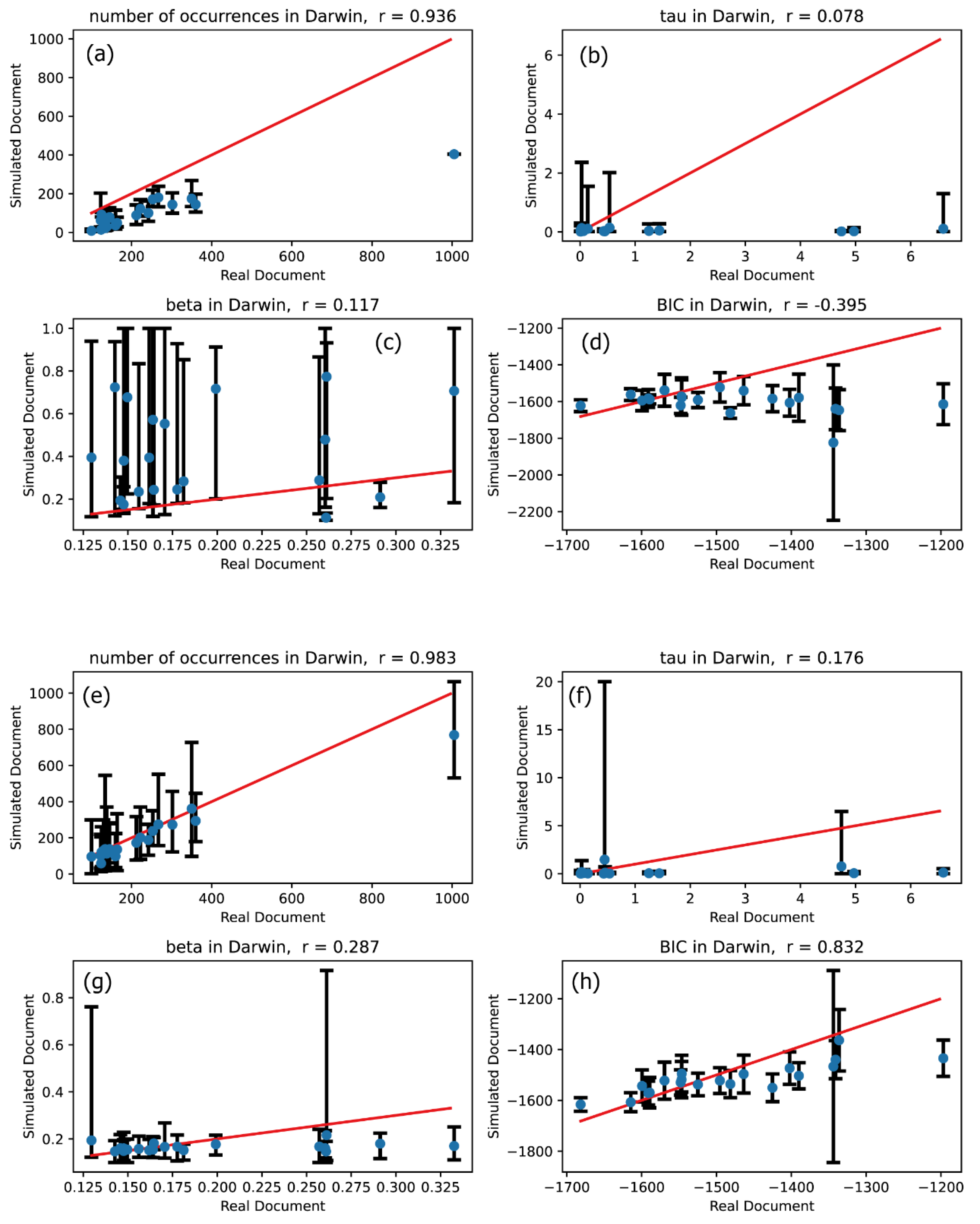
Figure 3.
The same meaning plots as in Figure 2 for Einstein text.
Figure 3.
The same meaning plots as in Figure 2 for Einstein text.
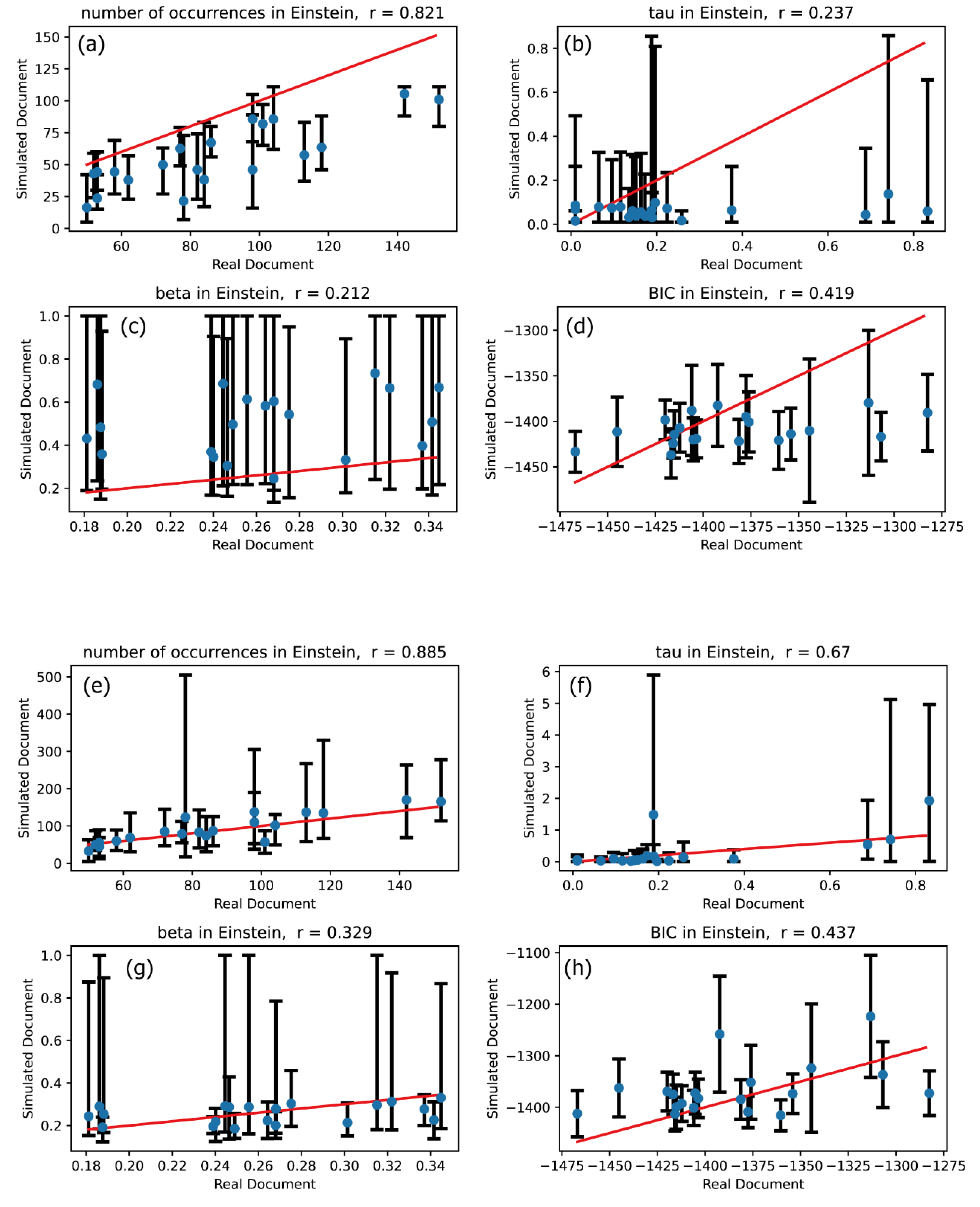
Figure 4.
The same meaning plots as in Figure 2 for Faraday text.
Figure 4.
The same meaning plots as in Figure 2 for Faraday text.
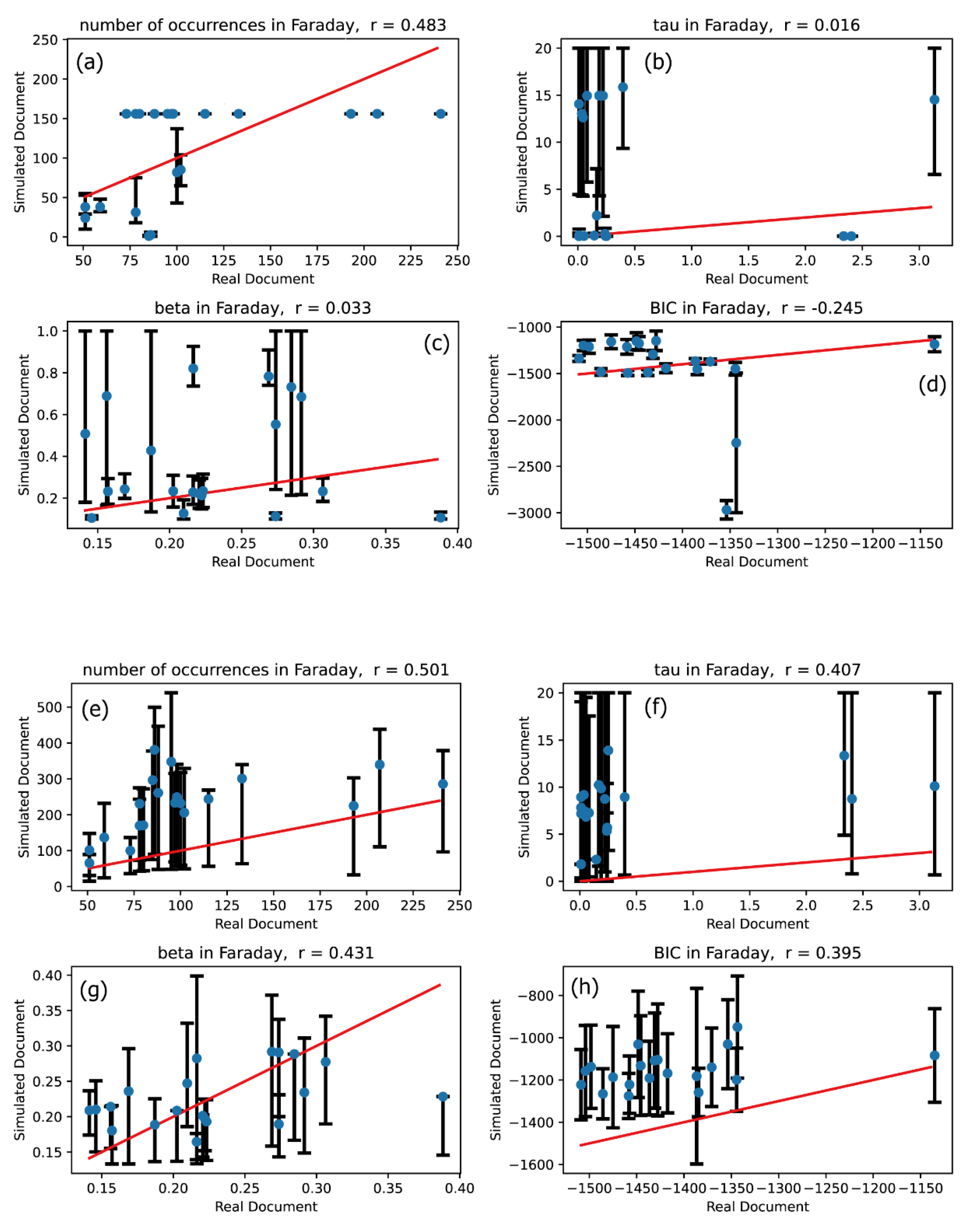
Figure 5.
The same meaning plots as in Figure 2 for Freud text.
Figure 5.
The same meaning plots as in Figure 2 for Freud text.
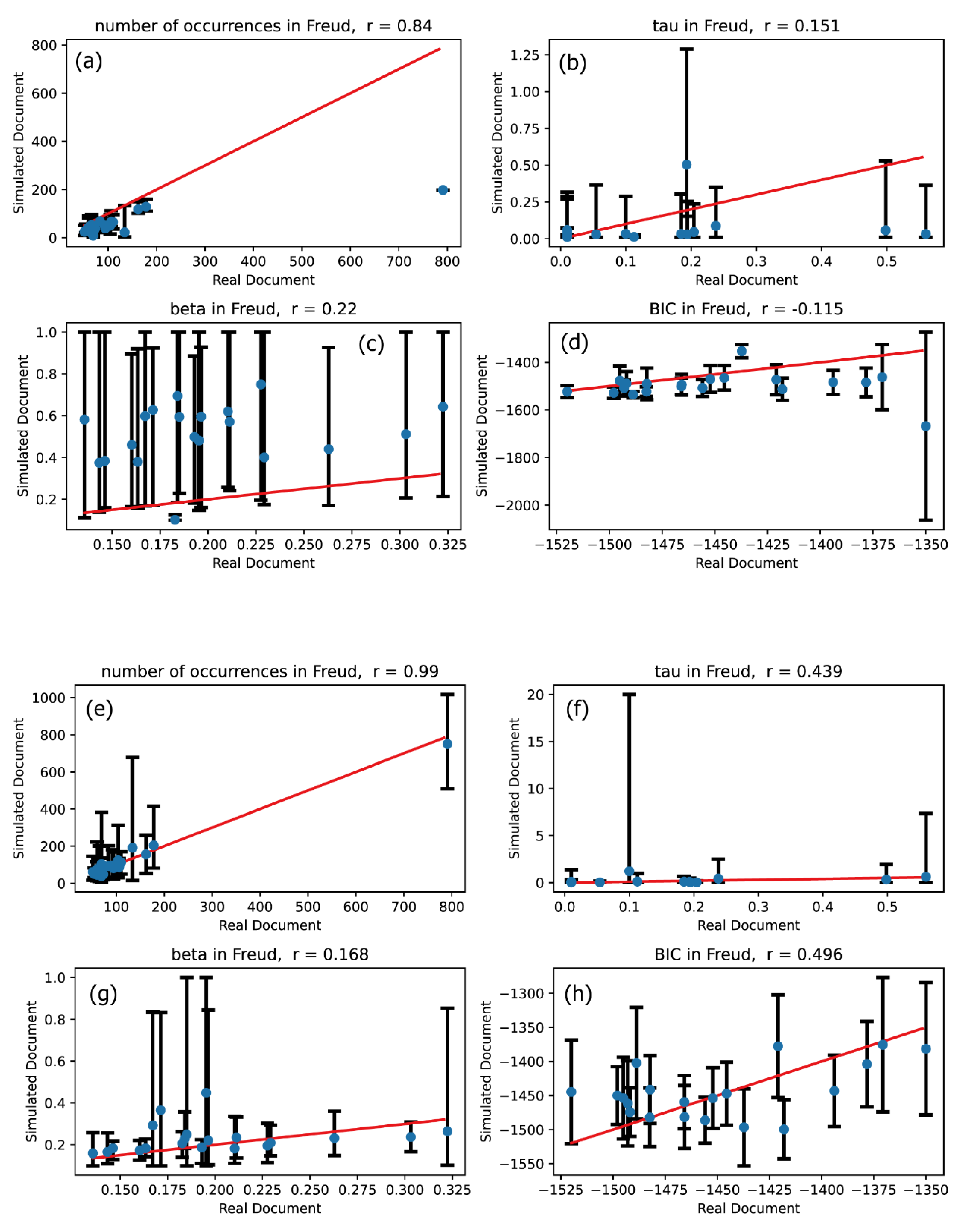
Figure 6.
Similar plots to those in Figure 2 are presented for the Paine text, except that an 8-dimensional multivariate Hawkes process was used to calculate the vertical quantities in plots (e)–(h).
Figure 6.
Similar plots to those in Figure 2 are presented for the Paine text, except that an 8-dimensional multivariate Hawkes process was used to calculate the vertical quantities in plots (e)–(h).
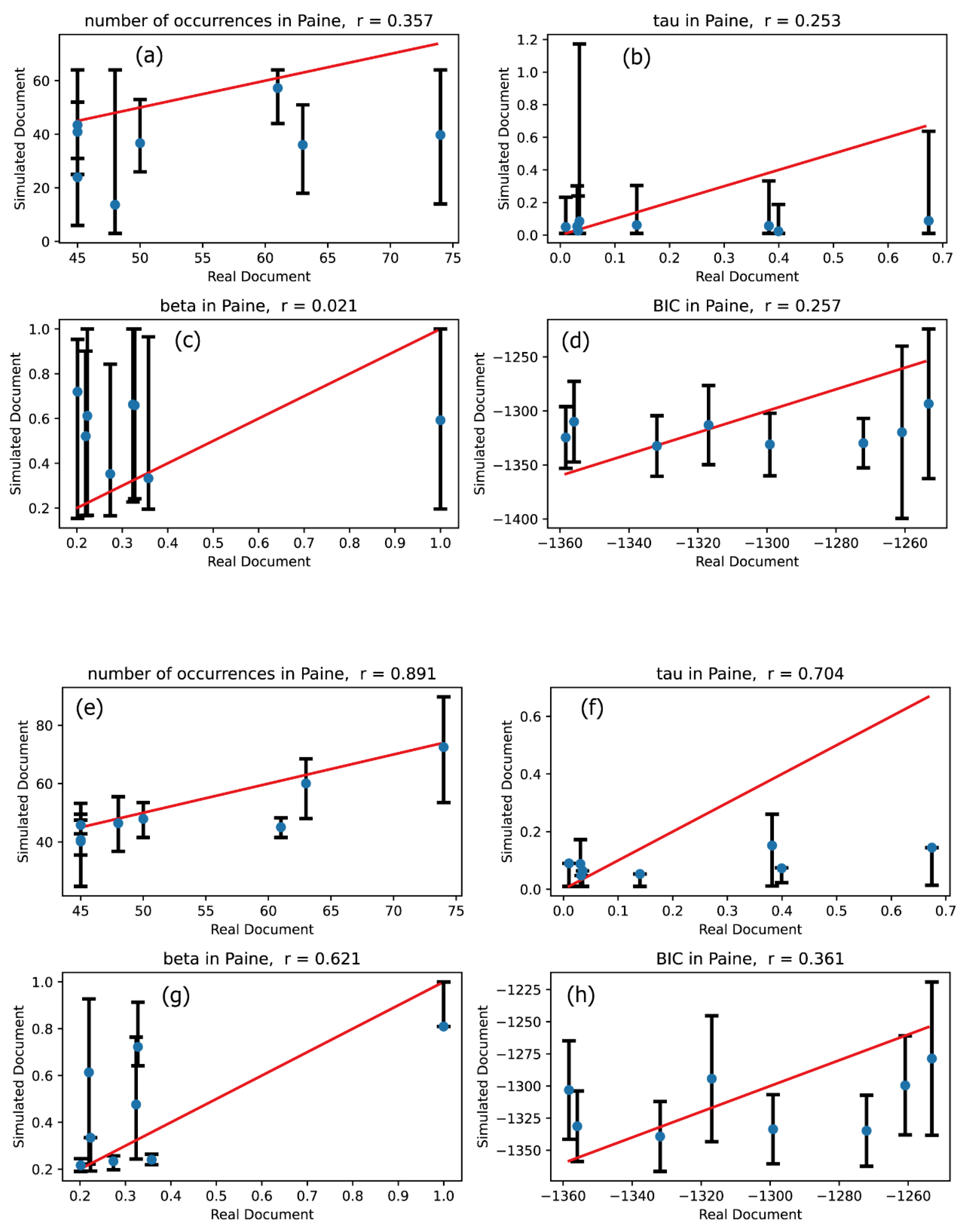
Figure 7.
The same meaning plots as in Figure 2 for Plato text.
Figure 7.
The same meaning plots as in Figure 2 for Plato text.
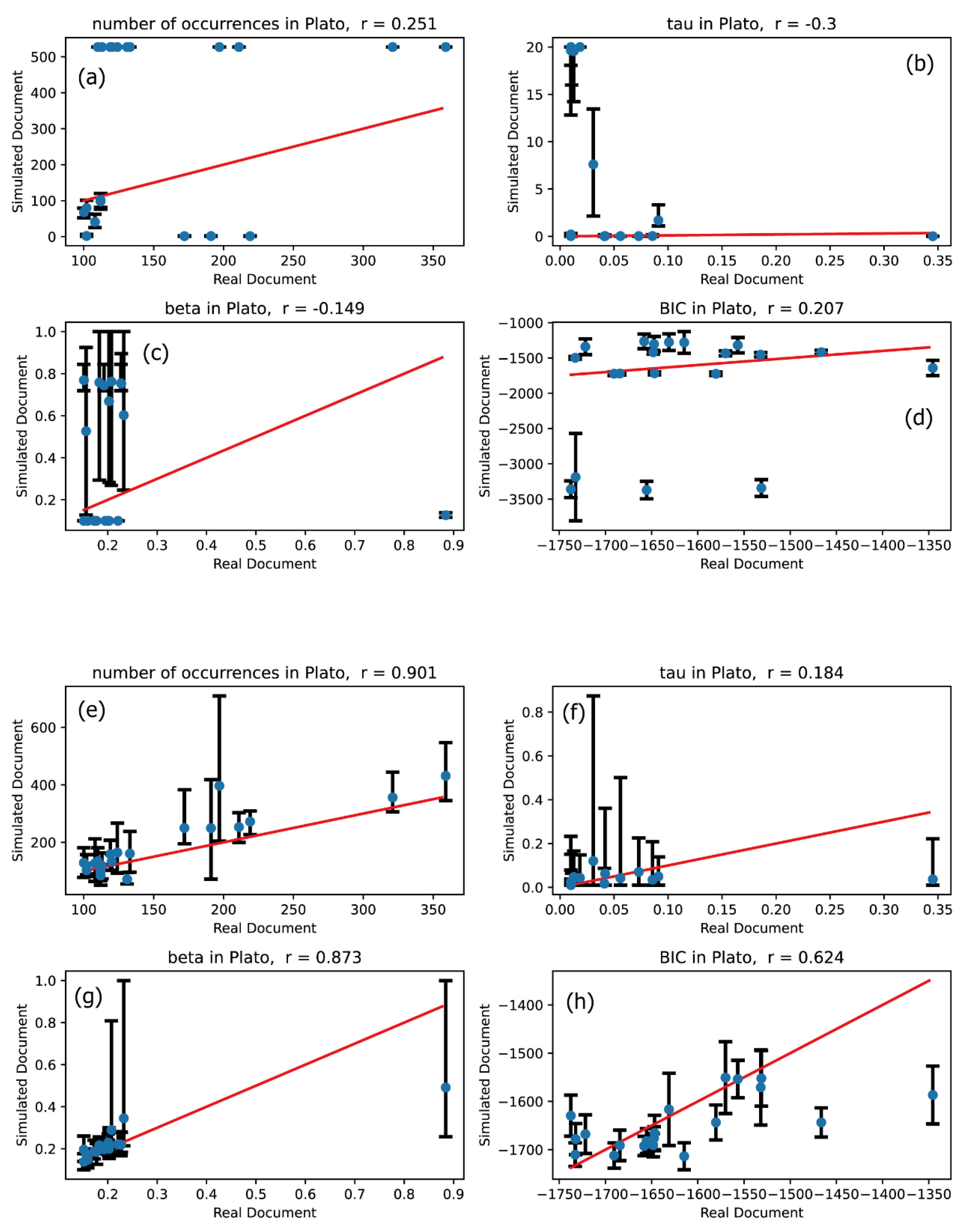
Our primary focus is to evaluate the extent to which the effectiveness of modeling improves when transitioning from the univariate Hawkes process to the multivariate Hawkes process. To assess this, we compared the description accuracies of the univariate Hawkes process and the multivariate Hawkes process across Figures 2 through 7: comparisons between plots (a) and (e) for the number of occurrences, between plots (b) and (f) for the relaxation time , between plots (c) and (g) for the shape parameter , and between plots (d) and (h) for the Bayesian Information Criterion (BIC).
These comparisons clearly demonstrate that the multivariate Hawkes process significantly enhances modeling effectiveness compared to the univariate Hawkes process. This improvement is evidenced by the scatter plots of the four characteristic quantities being distributed closer to the straight line in the case of the multivariate Hawkes process, with correlation coefficients approaching 1. Indeed, Table 3 confirms that the correlation coefficient for each quantity is closer to 1 when modeling with the multivariate Hawkes process is applied.
This result is unsurprising, given the nature of the document, which presents concepts each of which is explained by using multiple key terms. These key terms are frequently repeated throughout the explanation, creating inherent correlations among them. As a result, the multivariate Hawkes process effectively captures these relationships.
In contrast, the univariate Hawkes process is limited to capturing self-correlation, meaning it only reflects the correlations found within the occurrence signal of a single word.
3.2. Hawkes Graphs
Hawkes graphs are directed graphs that intuitively represent multivariate Hawkes processes. In these graphs, each node corresponds to a specific type of event in the multivariate Hawkes process, while each edge indicates how one type of event (represented at the root of the arrow) influences or enhances another type of event (located at the tip of the arrow). Examples of Hawkes graphs are presented in Figure 8 and Figure 9, which illustrate the multivariate Hawkes processes optimized to model word occurrence signals in the Paine text and the Plato text, respectively. Each node represents the occurrence events of an important word, and its corresponding background intensity, , as defined in Equation (5), is also displayed within the node.
In a multivariate Hawkes process, various types of events mutually excite one another, and the magnitude of their mutual excitation is quantified by the following coefficient [32]:
This coefficient measures how much the event of type- enhances the occurrence of the type- event. In Figure 8 and Figure 9, the values of are displayed alongside the edges. To improve readability, edges with are not shown in the graphs.
By constructing a Hawkes graph for a given text using the optimized parameter values of the multivariate Hawkes process, it becomes easier to infer the central concepts or notions of the text. For instance, based on Figure 8, we identify “time” as one of the central notions in the Paine text. This conclusion is drawn from observing that five edges associated with the “time” node are incoming arrows, while only one edge flows outward from this node. The predominance of incoming arrows indicates that the concepts represented by the source nodes are predominantly used to describe the notion of “time.”
3.3. Finding Important Notions in Texts
The idea for inferring the central notions of a text from the Hawkes graph, as mentioned above, can be refined as follows. The difference between the inflows into the -th node and the outflows from the same node is defined as:
This quantity intuitively represents the net extent to which the notion corresponding to the -th node is explained by other important notions.
The values of are displayed in Table 4, which ranks the importance of each notion in descending order for each text. The most important notion for each text—represented by the top-ranked word in Table 4—can be considered appropriately identified based on the content of each text, as will be discussed below.
Clearly, the notion of “species” in the Darwin text, “relativity” in the Einstein text, and “dream” in the Freud text are all closely tied to the main themes of the respective documents, serving as the central concepts each text seeks to explain. In the Faraday text, the principles of chemistry and physics are explored through the fascinating subject of candles. The most significant topic in the Faraday text is the investigation of the substances that constitute candles and how they transform during combustion. Thus, it is reasonable to identify “substance” as the most critical concept in the text. The Paine text is a groundbreaking pamphlet published during the American Revolution, emphasizing the urgency of declaring independence. In this text, the author employs the notion of “time” as a motivational framework for driving transformative action. Hence, “time” is regarded as central because the author explains the nature of the current “time” within this context. In the Plato text, the notion of “man” takes center stage because the author’s philosophical reflections on justice, governance, and enlightenment are deeply rooted in his understanding of human nature and elaborated upon through this perspective.
3.4. Advantages of Analyzing Texts with Multivariate Hawkes Processes
Based on the results outlined so far, the following advantages of utilizing the multivariate Hawkes process have been established:
- As demonstrated in Figures 2 through 7, the accuracy of modeling word occurrence signals in documents is significantly improved, making it more reliable when using the multivariate Hawkes process compared to the univariate one.
- A Hawkes graph can be generated from the parameter values obtained through the analysis using the multivariate Hawkes process. This facilitates an intuitive understanding of the relationships among the concepts that emerge in the document.
- The importance of each concept identified in a text can be assessed using the optimized parameters of the multivariate Hawkes process. The most significant concepts suggested for each text analyzed in this study are confirmed to be valid when considering the content of the text.
4. Conclusions
The occurrence signals of important words in six texts (one historical pamphlet and five renowned academic books) were modeled using univariate and multivariate Hawkes processes. The modeling procedure for the univariate Hawkes process was conducted as follows. First, optimized parameter values for the univariate Hawkes process were determined using maximum likelihood estimation (MLE) based on the occurrence signals of a given word in a considered text. Next, word occurrence signals were generated by simulating the univariate Hawkes process with optimized parameters. Finally, the validity of the univariate Hawkes process modeling was confirmed by verifying that the four characteristic quantities derived from the simulated word occurrence signals closely matched those obtained from the real signals observed in the text.
The modeling procedure for the multivariate Hawkes process followed a similar approach. First, optimized parameters for the -dimensional multivariate Hawkes process were evaluated using MLE based on the occurrence signals of important words, where represents the number of important words analyzed simultaneously with the multivariate Hawkes process. In this study, the typical value of was set to be 20. Next, occurrence signals of important words were simultaneously simulated using the multivariate Hawkes process with the optimized parameters. Finally, the validity of the multivariate Hawkes process modeling was confirmed by ensuring that the four characteristic quantities derived from the simulated word occurrence signals closely matched those obtained from the real signals observed in the text.
By validating the modeling with univariate and multivariate Hawkes processes, we observed that the correlation coefficients of the four characteristic quantities between real and simulated signals are notably closer to one in the case of the multivariate Hawkes process compared to the univariate one. This result demonstrates that the multivariate Hawkes process provides greater accuracy in describing word occurrence signals.
Additional advantages of the multivariate Hawkes process include its ability to intuitively represent the relationships among concepts described in a document through a Hawkes graph and to evaluate the importance of words in the text based on their relationships. For instance, the most important words in the analyzed documents were inferred using the optimized parameters of multivariate Hawkes processes, and these findings were confirmed to be valid.
Potential directions for future research utilizing the multivariate Hawkes process, which proved useful in this study, include:
- Enhancing the accuracy of word occurrence signal descriptions by increasing the number of important words analyzed simultaneously.
- Treating the matrix (defined by Equation (11)) as an adjacency matrix and applying graph theory methods, such as spectral clustering.
Since increasing the dimensionality of the multivariate Hawkes process poses challenges related to the computational cost of the MLE method, these directions are deferred to future studies.
Supplementary Materials
The Hawkes graphs for Darwin, Einstein, Faraday and Freud texts can be downloaded in the Open Science Framework repository at https://osf.io/6d8sf/files/osfstorage.
Author Contributions
For research articles with several authors, a short paragraph specifying their individual contributions must be provided. The following statements should be used “Conceptualization, H.O.; methodology, H.O.; software, H.O.; validation, Y.H., K.O. and M.K.; formal analysis, M.K.; investigation, H.O.; resources, H.O.; data curation, K.O.; writing—original draft preparation, H.O.; writing—review and editing, Y.H.; visualization, H.O. and K.O.; supervision, H.O.; project administration, H.O. and M.K.; funding acquisition, H.O. All authors have read and agreed to the published version of the manuscript.
Funding
This research was funded by JSPS KAKENHI, grant number 24K15198.
Institutional Review Board Statement
Not applicable.
Informed Consent Statement
Not applicable.
Data Availability Statement
Datasets and the major source codes used in this study are available in the Open Science Framework repository at https://osf.io/6d8sf/.
Conflicts of Interest
The authors declare no conflicts of interest.
Abbreviations
The following abbreviations are used in this manuscript:
| MLE | Maximum Likelihood Estimation |
| ACF | Autocorrelation Function |
| BIC | Bayesian Information Criterion |
| KWW | Kohlausch-Williams-Watts |
References
- Pawlowski, A. Time-Series Analysis in Linguistics. Application of the Arima Method to Some Cases of Spoken Polish. J. Quant. Linguist. 1997, 4, 203–221. [Google Scholar] [CrossRef]
- Pawlowski, A. Language in the Line vs. Language in the Mass: On the Efficiency of Sequential Modelling in the Analysis of Rhythm. J. Quant. Linguist. 1999, 6, 70–77. [Google Scholar] [CrossRef]
- Pawlowski, A. Modelling of Sequential Structures in Text. In Handbooks of Linguistics and Communication Science; Walter deGruyter: Berlin, Germany, 2005; pp. 738–750. [Google Scholar]
- Pawlowski, A.; Eder, M. Sequential Structures in “Dalimil’s Chronicle”; Mikros, G.K., Macutek, J., Eds.; Walter de Gruyter: Berlin, Germany, 2015; pp. 147–170. [Google Scholar] [CrossRef]
- Altmann, E.G.; Pierrehumbert, J.B.; Motter, A.E. Beyond word frequency: Bursts, lulls, and scaling in the temporal distributions of words. PLoS ONE 2009, 4, e7678. [Google Scholar] [CrossRef]
- Tanaka-Ishii, K.; Bunde, A. Long-range memory in literary texts: On the universal clustering of the rare words. PLoS ONE 2016, 11, e0164658. [Google Scholar] [CrossRef]
- Schenkel, A.; Zhang, J.; Zhang, Y. Long range correlation in human writings. Fractals 1993, 1, 47–57. [Google Scholar] [CrossRef]
- Ebeling, W.; Pöschel, T. Entropy and long-range correlations in literary english. Europhys. Lett. 1994, 26, 241. [Google Scholar] [CrossRef]
- Montemurro, M.A.; Pury, P.A. Long-range fractal correlations in literary corpora. Fractals 2002, 10, 451–461. [Google Scholar] [CrossRef]
- Alvarez-Lacalle, E.; Dorow, B.; Eckmann, J.P.; Moses, E. Hierarchical structures induce long-range dynamic correlations in written texts. Proc. Natl. Acad. Sci. USA 2006, 103, 7956–7961. [Google Scholar] [CrossRef]
- Altmann, E.G.; Cristadoro, G.; Esposti, M.D. On the origin of long-range correlations in texts. Proc. Natl. Acad. Sci. USA 2012, 109, 11582–11587. [Google Scholar] [CrossRef]
- Chatzigeorgiou, M.; Constantoudis, V.; Diakonos, F.; Karamanos, K.; Papadimitriou, C.; Kalimeri, M.; Papageorgiou, H. Multifractal correlations in natural language written texts: Effects of language family and long word statistics. Physica. A 2017, 469, 173–182. [Google Scholar] [CrossRef]
- Ogura, H.; Amano, H.; Kondo, M. Measuring Dynamic Correlations of Words in Written Texts with an Autocorrelation Function. J. Data Anal. Inf. Process 2019, 7, 46–73. [Google Scholar] [CrossRef]
- Ogura, H.; Amano, H.; Kondo, M. Origin of Dynamic Correlations of Words in Written Texts. J. Data Anal. Inf. Process. 2019, 7, 228–249. [Google Scholar] [CrossRef]
- Ogura, H.; Amano, H.; Kondo, M. Simulation of pseudo-text synthesis for generating words with long-range dynamic correlations. SN Appl. Sci. 2020, 2, 1387. [Google Scholar] [CrossRef]
- Ogura, H.; Hanada, Y.; Amano, H.; Kondo, M. A stochastic model of word occurrences in hierarchically structured written texts. SN Appl. Sci. 2022, 4, 77. [Google Scholar] [CrossRef]
- Ogura, H.; Hanada, Y.; Amano, H.; Kondo, M. Modeling Long-Range Dynamic Correlations of Words in Written Texts with Hawkes Processes. Entropy 2022, 24, 858. [Google Scholar] [CrossRef]
- Hawkes, A.G. Spectra of Some Self-Exciting and Mutually Exciting Point Processes. Biometrika 1971, 58, 83–90. [Google Scholar] [CrossRef]
- Ogata, Y. Statistical models for earthquake occurrences and residual analysis for point processes. J. Amer. Statist. Assoc. 1988, 83, 9–27. [Google Scholar] [CrossRef]
- Ogata, Y. Seismicity analysis through point-process modeling: A review. Pure Appl. Geophys. 1999, 155, 471–507. [Google Scholar] [CrossRef]
- Zhuang, J.; Ogata, Y.; Vere-Jones, D. Stochastic declustering of space-time earthquake occurrences. J. Amer. Statist. Soc. 2002, 97, 369–380. [Google Scholar] [CrossRef]
- Truccolo, W.; Eden, U.T.; Fellows, M.R.; Donoghue, J.P.; Brown, E.N. A Point Process Framework for Relating Neural Spiking Activity to SpikingHistory, Neural Ensemble, and Extrinsic Covariate Effects. J. Neurophysiol. 2005, 93, 1074–1089. [Google Scholar] [CrossRef]
- Reynaud-Bouret, P.; Rivoirard, V.; Tuleau-Malot, C. Inference of functional connectivity in Neurosciences via Hawkes processes. In Proceedings of the 1st IEEE Global Conference on Signal and Information Processing, Austin, TX, USA, 3–5 December 2013. [Google Scholar] [CrossRef]
- Gerhard, F.; Deger, M.; Truccolo, W. On the stability and dynamics of stochastic spiking neuron models: Nonlinear Hawkes process and point process GLMs. PLoS Comput. Biol. 2017, 13, e1005390. [Google Scholar] [CrossRef] [PubMed]
- Bacry, E.; Mastromatteo, I.; Muzy, J. Hawkes Processes in Market. Microstruct. Liq. 2015, 1, 1550005. [Google Scholar] [CrossRef]
- Rizoiu, M.A.; Lee, Y.; Mishra, S.; Xie, L. Hawkes processes for events in social media. In Frontiers of Multimedia. In Frontiers of Multimedia Research, 1st ed.; Chang, S. 2017, Ed.; Association for Computing Machinery and Morgan & Claypool: New York, USA, 2017. [Google Scholar] [CrossRef]
- Palmowski, Z.; Puchalska, D. Modeling social media contagion using Hawkes processes. J. Pol. Math. Soc. 2021, 49, 65–83. [Google Scholar] [CrossRef]
- Chiang, W.H.; Liu, X.; Mohler, G. Hawkes process modeling of COVID-19 with mobility leading indicators and spatial covariates. Int. J. Forecast. 2022, 38, 505–520. [Google Scholar] [CrossRef]
- Embrechts, P.; Liniger, T. ; Lin. L. Multivariate Hawkes processes: an application to financial data. J. Appl. Probab. 2011, 48, 367–378. [Google Scholar] [CrossRef]
- Bowsher, C. G. Modelling security market events in continuous time: Intensity based, multivariate point process models, J. Econom 2007, 141, 876–912. [Google Scholar] [CrossRef]
- Yang, S. Y.; Liu, A. ; Chen, J;. Hawkes, A. Applications of a multivariate Hawkes process to joint modeling of sentiment and market return events, Quant. Finance 2018, 18(2), 295–310. [CrossRef]
- Embrechts, P.; Kirchner, M. Hawkes graphs, Theory Probab. Its Appl. 62, 132–156. [CrossRef]
- Osman, A. H.; Barukub, O. M. , Graph-Based Text Representation and Matching: A Review of the State of the Art and Future Challenges, IEEE Access 2020, 8, 87562–87583. [CrossRef]
- Edited by Segev, E. Semantic Network Analysis in Social Sciences, 1st ed.; Taylor & Francis, New York, USA, 2022.
- Laub, P. J.; Taimre, T.; Pollett. P.; Taimre, T. Hawkes Processes, arXiv:1507.02822. 2015. [CrossRef]
- Laub, P. J.; Lee, Y.; Pollett, K. P.; Taimre, T. Hawkes Models and Their Applications, arXiv:2405.10527. 2024. arXiv:2405.10527. 2024.
- Lindström,A.; Lindgren, S.; Sainudiin, R. Hawkes Processes on Social and Mass Media, International Conference on Data Technologies and Applications 2023, https://uu.diva-portal.org/smash/get/diva2:1827189/FULLTEXT01.pdf.
- Daley, D. J.; Vere-Jones, D. An Introduction to the Theory of Point Processes: Volume I :Elementary Theory and Methods, 2nd ed.; Springer-Verlag, New York, USA, 2003.
Figure 1.
(a) The word occurrence signal, , for the word “formation” in the Darwin text, and (b) the calculated ACFs (circles) along with the fitted KWW function to the ACFs (red curve) for the word “formation” in the Darwin text.
Figure 1.
(a) The word occurrence signal, , for the word “formation” in the Darwin text, and (b) the calculated ACFs (circles) along with the fitted KWW function to the ACFs (red curve) for the word “formation” in the Darwin text.
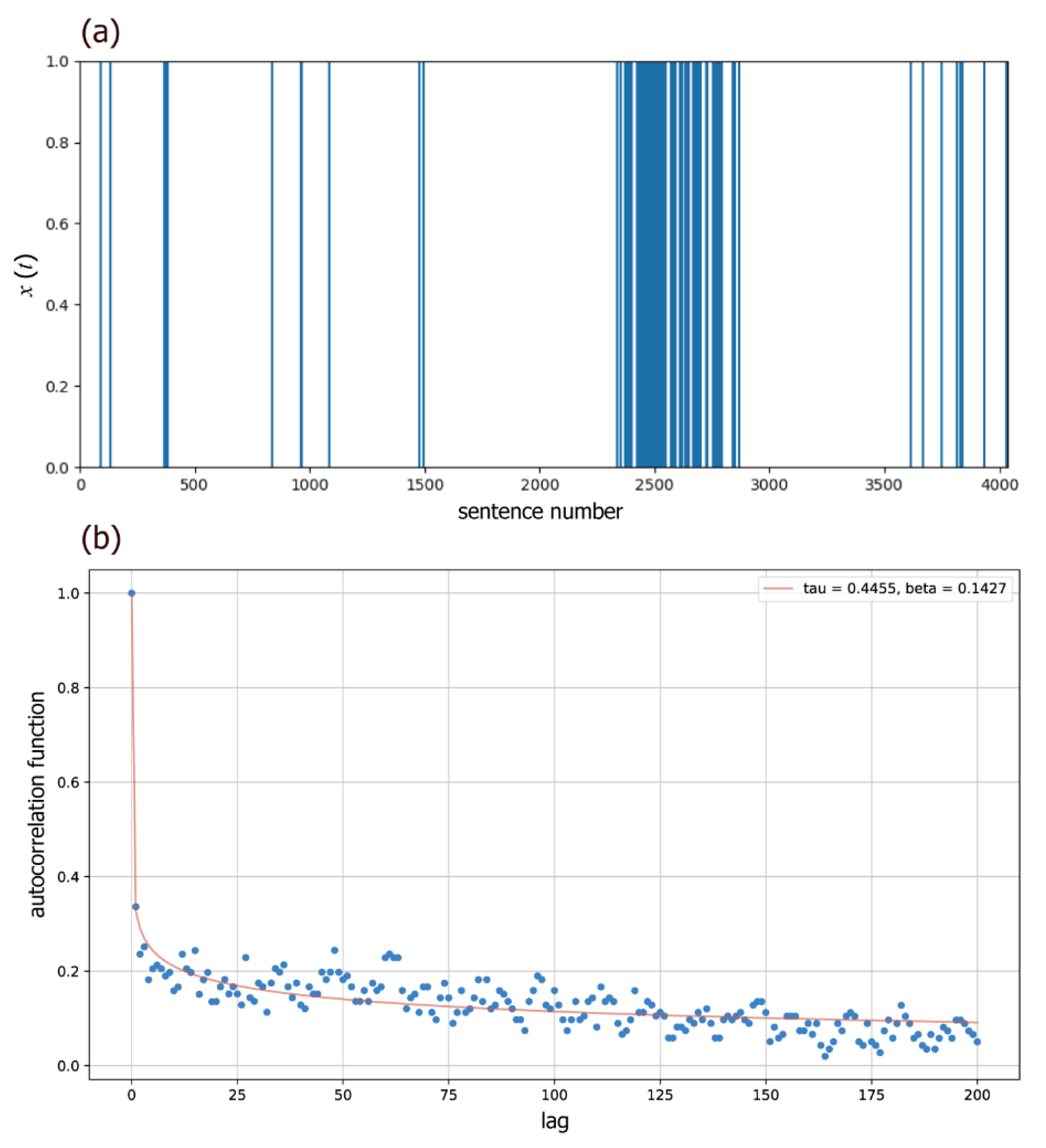
Figure 8.
Figure 8. An example of a Hawkes graph representing the Paine text. The numbers near the arrows indicate the values of defined by Equation (11) while the numbers within the nodes represent the background intensities . The colors of the nodes and arrows are shaded such that higher values of and result in darker nodes and arrows.
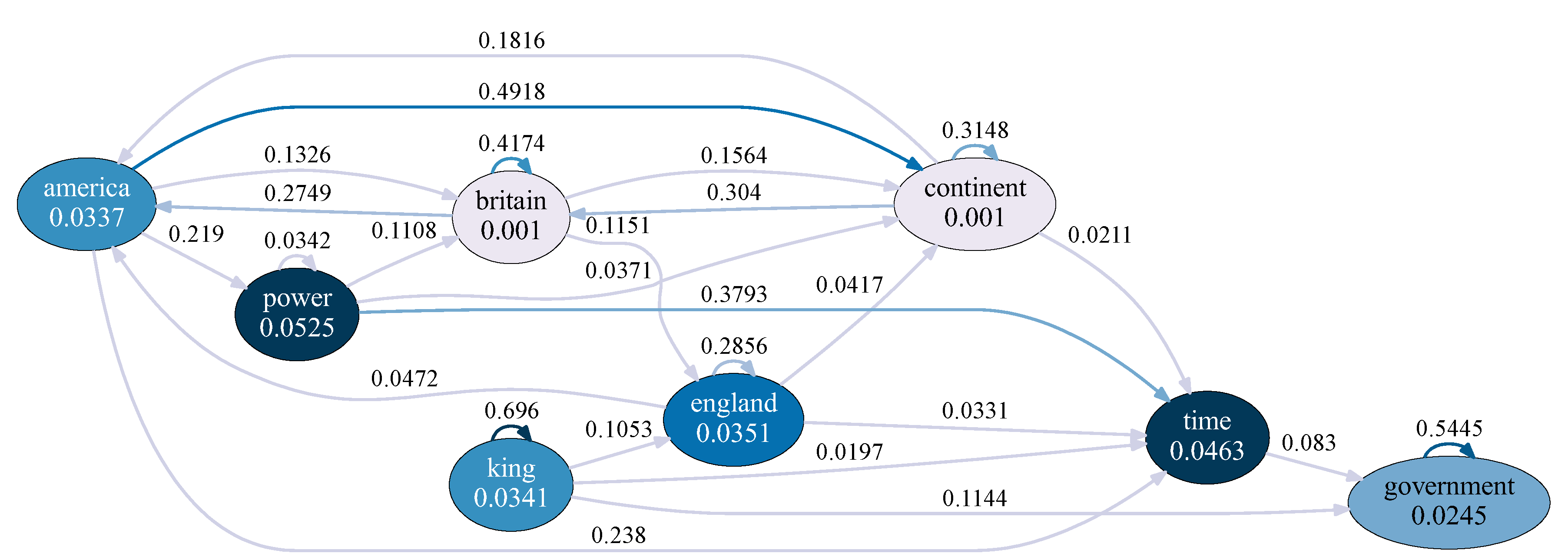
Figure 9.
Figure 9. An example of a Hawkes graph representing the Plato text.
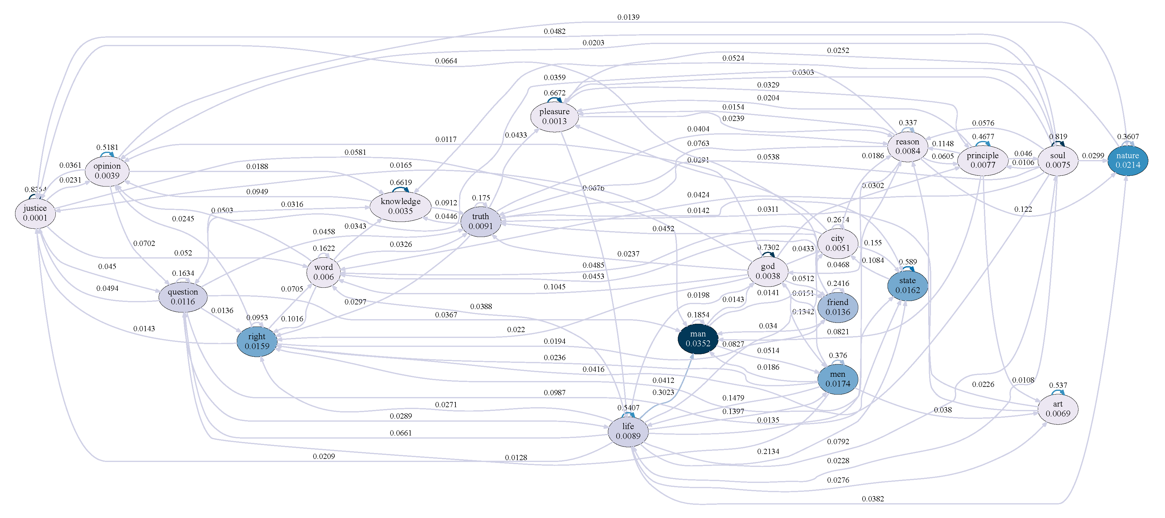

Table 1.
Summary of English texts employed.
| Short Name | Title | Author | Vocabulary Size | Length in Sentences |
|---|---|---|---|---|
| Darwin | On the Origin of Spiecies | Charles Darwin | 5728 | 4036 |
| Einstein | Relativity: The Special and General Theory | Albert Einstein | 2222 | 1107 |
| Faraday | The Chemical History of a Candl | Michael Faraday | 1563 | 2563 |
| Freud | Dream Psychology | Sigmund Freud | 4520 | 1977 |
| Paine | Common Sense | Thomas Paine | 637 | 2558 |
| Plato | The Republic | Plato | 5686 | 5268 |
Table 2.
The top 20 important words for each text. Note that for the Paine text, the selected words are limited to only 8, as the text is significantly shorter than the others. We relaxed the criteria to 45 or more occurrences instead of 50 or more, but only eight words met that criterion for the Paine text.
| Text | Word | number of Occurrences | |||
|---|---|---|---|---|---|
| Darwin | formation | 134 | 0.446 | 0.143 | 2280.488 |
| hybrid | 124 | 4.971 | 0.199 | 617.345 | |
| cross | 160 | 0.534 | 0.171 | 297.335 | |
| class | 123 | 0.010 | 0.130 | 220.608 | |
| selection | 350 | 0.029 | 0.148 | 91.912 | |
| instinct | 100 | 4.744 | 0.261 | 88.223 | |
| group | 212 | 0.140 | 0.181 | 41.714 | |
| island | 138 | 6.593 | 0.333 | 39.887 | |
| period | 267 | 0.010 | 0.146 | 37.960 | |
| world | 145 | 0.010 | 0.148 | 31.846 | |
| organ | 164 | 1.438 | 0.260 | 27.215 | |
| production | 125 | 0.010 | 0.150 | 26.628 | |
| plant | 302 | 0.062 | 0.178 | 22.628 | |
| structure | 222 | 0.015 | 0.156 | 22.617 | |
| habit | 145 | 0.020 | 0.162 | 19.592 | |
| variety | 360 | 1.250 | 0.291 | 13.272 | |
| part | 253 | 0.013 | 0.165 | 11.025 | |
| character | 242 | 0.454 | 0.257 | 9.247 | |
| theory | 130 | 0.010 | 0.164 | 8.650 | |
| specie | 1005 | 0.429 | 0.261 | 8.021 | |
| Einstein | velocity | 84 | 0.143 | 0.188 | 30.516 |
| field | 78 | 0.832 | 0.275 | 11.681 | |
| light | 82 | 0.196 | 0.239 | 6.240 | |
| body | 113 | 0.189 | 0.240 | 5.845 | |
| equation | 50 | 0.741 | 0.322 | 5.092 | |
| motion | 98 | 0.188 | 0.246 | 4.932 | |
| position | 53 | 0.173 | 0.245 | 4.751 | |
| theory | 142 | 0.688 | 0.337 | 3.958 | |
| place | 58 | 0.010 | 0.181 | 2.977 | |
| co-ordinate | 86 | 0.152 | 0.264 | 2.646 | |
| point | 104 | 0.115 | 0.256 | 2.429 | |
| law | 118 | 0.258 | 0.301 | 2.341 | |
| line | 52 | 0.010 | 0.186 | 2.298 | |
| relativity | 152 | 0.135 | 0.268 | 2.184 | |
| reference | 72 | 0.010 | 0.188 | 2.067 | |
| principle | 62 | 0.375 | 0.342 | 2.058 | |
| time | 98 | 0.065 | 0.249 | 1.601 | |
| space | 77 | 0.095 | 0.268 | 1.535 | |
| distance | 53 | 0.163 | 0.315 | 1.221 | |
| system | 101 | 0.224 | 0.345 | 1.188 | |
| Faraday | flame | 133 | 0.396 | 0.169 | 247.670 |
| candle | 241 | 0.081 | 0.157 | 115.727 | |
| jar | 78 | 0.011 | 0.141 | 62.389 | |
| gas | 97 | 0.010 | 0.146 | 37.606 | |
| carbon | 85 | 2.335 | 0.269 | 37.103 | |
| water | 193 | 2.403 | 0.274 | 34.772 | |
| oxygen | 115 | 3.134 | 0.306 | 26.441 | |
| heat | 95 | 0.187 | 0.203 | 20.215 | |
| acid | 86 | 0.252 | 0.216 | 16.023 | |
| atmosphere | 51 | 0.010 | 0.156 | 15.353 | |
| hydrogen | 78 | 0.167 | 0.210 | 13.548 | |
| air | 207 | 0.221 | 0.223 | 11.207 | |
| iron | 59 | 0.242 | 0.292 | 2.556 | |
| combustion | 98 | 0.045 | 0.222 | 2.357 | |
| experiment | 100 | 0.010 | 0.187 | 2.184 | |
| piece | 88 | 0.035 | 0.221 | 1.910 | |
| vessel | 51 | 0.145 | 0.285 | 1.716 | |
| action | 80 | 0.238 | 0.388 | 0.862 | |
| substance | 102 | 0.054 | 0.274 | 0.774 | |
| part | 73 | 0.010 | 0.216 | 0.639 | |
| Freud | psychic | 134 | 0.100 | 0.136 | 1081.268 |
| dream | 791 | 0.193 | 0.183 | 52.727 | |
| process | 104 | 0.010 | 0.143 | 48.251 | |
| content | 110 | 0.010 | 0.146 | 36.565 | |
| system | 69 | 0.560 | 0.228 | 24.712 | |
| wish | 178 | 0.238 | 0.211 | 18.195 | |
| consciousness | 65 | 0.112 | 0.196 | 15.783 | |
| thought | 162 | 0.194 | 0.210 | 15.365 | |
| work | 69 | 0.010 | 0.160 | 11.299 | |
| analysis | 92 | 0.010 | 0.163 | 9.023 | |
| sleep | 94 | 0.498 | 0.263 | 8.937 | |
| activity | 60 | 0.010 | 0.167 | 6.947 | |
| formation | 51 | 0.010 | 0.171 | 5.324 | |
| interpretation | 54 | 0.010 | 0.184 | 2.549 | |
| life | 83 | 0.010 | 0.185 | 2.419 | |
| day | 106 | 0.054 | 0.229 | 2.277 | |
| state | 66 | 0.010 | 0.193 | 1.640 | |
| child | 73 | 0.185 | 0.303 | 1.634 | |
| form | 60 | 0.010 | 0.195 | 1.475 | |
| idea | 69 | 0.204 | 0.322 | 1.394 | |
| Paine | king | 74 | 0.674 | 0.274 | 9.774 |
| continent | 48 | 0.035 | 0.202 | 3.942 | |
| government | 63 | 0.399 | 0.358 | 1.866 | |
| britain | 45 | 0.031 | 0.223 | 1.577 | |
| england | 50 | 0.140 | 0.323 | 0.944 | |
| america | 45 | 0.010 | 0.220 | 0.571 | |
| time | 61 | 0.382 | 0.999 | 0.382 | |
| power | 45 | 0.033 | 0.327 | 0.209 | |
| Plato | justice | 191 | 0.056 | 0.152 | 126.257 |
| god | 124 | 0.031 | 0.151 | 70.764 | |
| pleasure | 108 | 0.041 | 0.156 | 64.617 | |
| knowledge | 133 | 0.042 | 0.177 | 15.639 | |
| soul | 197 | 0.013 | 0.159 | 15.349 | |
| opinion | 100 | 0.086 | 0.202 | 9.287 | |
| state | 359 | 0.018 | 0.172 | 9.145 | |
| art | 113 | 0.091 | 0.221 | 5.013 | |
| life | 172 | 0.073 | 0.227 | 3.330 | |
| principle | 102 | 0.010 | 0.183 | 2.716 | |
| men | 219 | 0.010 | 0.192 | 1.687 | |
| nature | 211 | 0.010 | 0.195 | 1.496 | |
| city | 110 | 0.010 | 0.196 | 1.410 | |
| reason | 119 | 0.011 | 0.201 | 1.241 | |
| man | 321 | 0.010 | 0.201 | 1.155 | |
| truth | 120 | 0.010 | 0.203 | 1.080 | |
| friend | 112 | 0.010 | 0.207 | 0.891 | |
| word | 102 | 0.010 | 0.227 | 0.447 | |
| question | 112 | 0.010 | 0.232 | 0.384 | |
| right | 131 | 0.345 | 0.884 | 0.367 |
Table 3.
Comparison of the correlation coefficients for the four characteristic quantities. Each coefficient indicates the degree of correlation between the real and simulated word occurrence signals for the given quantity. The simulated signals are generated using either univariate or multivariate Hawkes processes, and both cases are presented in the table for comparison.
| text | number of occurrences | BIC | ||||||||
|---|---|---|---|---|---|---|---|---|---|---|
| univariate | multivariate | univariate | multivariate | univariate | multivariate | univariate | multivariate | |||
| Darwin | 0.936 | 0.983 | 0.078 | 0.176 | 0.117 | 0.287 | -0.395 | 0.832 | ||
| Einstein | 0.821 | 0.885 | 0.237 | 0.670 | 0.212 | 0.329 | 0.419 | 0.437 | ||
| Faraday | 0.483 | 0.501 | 0.016 | 0.407 | 0.033 | 0.431 | -0.245 | 0.395 | ||
| Freud | 0.840 | 0.990 | 0.151 | 0.439 | 0.220 | 0.168 | -0.115 | 0.496 | ||
| Paine | 0.357 | 0.891 | 0.253 | 0.764 | 0.021 | 0.621 | 0.257 | 0.361 | ||
| Plato | 0.251 | 0.901 | -0.300 | 0.184 | -0.149 | 0.873 | 0.207 | 0.624 | ||
Table 4.
The difference between inflows and outflows, for each important notion. Each row is arranged in descending order of .
Table 4.
The difference between inflows and outflows, for each important notion. Each row is arranged in descending order of .
| Darwin | Einstein | Freud | |||||
| node | node | node | |||||
| species | 1.1250 | relativity | 0.8213 | dream | 2.0732 | ||
| period | 0.7721 | law | 0.7765 | life | 0.7262 | ||
| selection | 0.2300 | light | 0.7715 | form | 0.4541 | ||
| cross | 0.2029 | body | 0.6530 | analysis | 0.3601 | ||
| plant | 0.1817 | system | 0.5132 | thought | 0.3168 | ||
| theory | 0.1802 | time | 0.4872 | process | 0.2235 | ||
| part | 0.1603 | point | 0.2187 | state | 0.1755 | ||
| class | 0.0453 | reference | 0.2175 | day | 0.1222 | ||
| habit | -0.0095 | place | -0.0674 | consciousness | 0.1075 | ||
| world | -0.0652 | space | -0.0780 | idea | 0.0348 | ||
| structure | -0.0659 | motion | -0.2615 | sleep | -0.0057 | ||
| character | -0.0694 | co-ordinate | -0.3237 | wish | -0.0366 | ||
| island | -0.1285 | principle | -0.3451 | formation | -0.1510 | ||
| group | -0.1385 | field | -0.3476 | activity | -0.2573 | ||
| variety | -0.1548 | line | -0.3938 | system | -0.3008 | ||
| instinct | -0.1672 | distance | -0.4206 | psychic | -0.3025 | ||
| organ | -0.2482 | theory | -0.4460 | interpretation | -0.3127 | ||
| hybrid | -0.4656 | position | -0.4774 | content | -0.5062 | ||
| production | -0.5281 | velocity | -0.5738 | work | -0.7205 | ||
| formation | -0.8565 | equation | -0.7238 | child | -2.0006 | ||
| Faraday | Paine | Plato | |||||
| node | node | node | |||||
| substance | 0.5210 | time | 0.6041 | man | 0.4548 | ||
| combustion | 0.4490 | continent | 0.2181 | state | 0.4078 | ||
| experiment | 0.3492 | government | 0.1954 | truth | 0.2285 | ||
| action | 0.3126 | england | 0.0994 | word | 0.1753 | ||
| air | 0.3018 | britain | 0.0010 | nature | 0.1652 | ||
| piece | 0.2421 | king | -0.2363 | opinion | 0.0921 | ||
| part | 0.1817 | power | -0.3051 | right | 0.0841 | ||
| water | 0.1041 | america | -0.5766 | men | 0.0721 | ||
| candle | 0.0081 | justice | 0.0658 | ||||
| carbon | -0.0058 | pleasure | 0.0433 | ||||
| gas | -0.0113 | art | 0.0269 | ||||
| vessel | -0.0677 | knowledge | -0.0127 | ||||
| atmosphere | -0.0687 | city | -0.0275 | ||||
| jar | -0.0965 | question | -0.0759 | ||||
| oxygen | -0.1220 | reason | -0.0761 | ||||
| flame | -0.1878 | friend | -0.1050 | ||||
| hydrogen | -0.2463 | principle | -0.1391 | ||||
| iron | -0.4329 | soul | -0.2651 | ||||
| heat | -0.5906 | god | -0.3241 | ||||
| acid | -0.6399 | life | -0.7905 | ||||
Disclaimer/Publisher’s Note: The statements, opinions and data contained in all publications are solely those of the individual author(s) and contributor(s) and not of MDPI and/or the editor(s). MDPI and/or the editor(s) disclaim responsibility for any injury to people or property resulting from any ideas, methods, instructions or products referred to in the content. |
© 2025 by the authors. Licensee MDPI, Basel, Switzerland. This article is an open access article distributed under the terms and conditions of the Creative Commons Attribution (CC BY) license (http://creativecommons.org/licenses/by/4.0/).
Copyright: This open access article is published under a Creative Commons CC BY 4.0 license, which permit the free download, distribution, and reuse, provided that the author and preprint are cited in any reuse.


