
Submitted:
21 May 2025
Posted:
22 May 2025
You are already at the latest version
Abstract
We present a scalable approach for quantum simulation of large proteins based on systematic fragmentation into amino acids or peptides, followed by independent quantum simulations and chemically guided reassembly. Using the QMProt dataset, we train regression models to estimate qubit and coefficient demands from electron count, and predict Toffoli gate counts via the SelectSwap algorithm. For systems up to 1852 electrons, our method achieves relative errors below 3\% and reduces gate requirements by up to $10^{20}$ compared to monolithic simulations, highlighting its potential for fault-tolerant simulation of biologically relevant molecules.
Keywords:
Quantum Computing
; Protein Simulation
; Fragmentation
; Toffoli Optimization
; Resource Estimation
; Glucagon
1. Introduction
Quantum simulation of biomolecular systems remains a major computational challenge due to the exponential scaling associated with solving the electronic Schrödinger equation. Proteins, in particular, present a formidable case, as they involve a large number of electrons and complex many-body interactions. Fragmentation techniques, which decompose macromolecules into smaller subsystems such as amino acids or peptides, have emerged as a viable approach to reduce computational overhead while preserving physical accuracy [1].
Quantum computing offers theoretical advantages in simulating electronic structure problems, where classical methods rapidly become intractable with system size [2,3]. By encoding quantum states directly in qubit-based representations, quantum computers avoid the combinatorial explosion characteristic of classical full configuration interaction methods. Despite the availability of approximations such as DFT [4] and CAS-CI [5], these approaches face well-known limitations in accuracy or scalability, particularly for systems with strong electronic correlation [6,7].
Exact quantum chemical simulations remain out of reach for full protein systems, even with quantum hardware. As such, methodologically principled reductions in problem size are essential. Our objective is to evaluate a fragmentation-based framework for scalable quantum simulation of proteins, balancing error control with computational feasibility. The methodology builds on our prior work [1], which introduced a reassembly scheme for independently simulated fragments with chemical corrections. That work demonstrated high accuracy on small peptides, achieving relative errors of approximately for amino acid-level fragmentation and for finer subdivisions.
In this study, we extend the methodology to larger and biologically relevant peptides, including Glucagon, Oxytocin, Vasopressin, and Angiotensin II, which vary in electron count and structural complexity. Among them, Glucagon stands out as a critical benchmark due to its physiological role and its size, comprising 29 amino acids and over 1800 electrons. Its simulation requires addressing more than coefficients, posing a stringent test for the scalability of our approach.
By systematically evaluating prediction errors and quantum resource estimates across these molecules, we aim to assess the practical applicability of fragmentation-based strategies for quantum chemistry. This work contributes to the broader effort of making accurate electronic structure simulations tractable for systems of biological and chemical relevance. Beyond molecular simulation, the methodology has potential implications in areas such as drug discovery and materials design, where electronic structure accuracy is essential and classical methods face intrinsic limitations.
The structure of the paper is as follows: Section 2 reviews related work in quantum simulation and fragmentation-based methods. Section 3 introduces our methodology, including regression models, Toffoli gate estimation, and the proposed multi-level fragmentation and reassembly strategy. Section 4 presents experimental validation on a range of peptides and proteins, from small dipeptides to large systems such as Glucagon, along with detailed error and scalability analyses. Section 5 discusses limitations, compares with alternative techniques, and outlines practical implications and future research. Section 6 summarizes our main findings and perspectives. Additional technical derivations and regression diagnostics are provided in the appendices.
2. Related Works
Quantum simulations of biomolecules have progressed along two converging lines: (i) classical fragment-based electronic-structure methods that exploit locality to curb cost, and (ii) quantum algorithms that aggressively compress qubit and gate resources. Our work positions itself at this intersection, extending classical fragmentation ideas into the quantum era and knitting together the most effective resource-optimisation tools reported to date.
Fragmentation approaches such as the Fragment Molecular Orbital (FMO) method [8], Our N-Layered Integrated Molecular Orbital and Molecular Mechanics (ONIOM) [9], and adaptive Quantum Mechanics/Molecular Mechanics (QM/MM) [10] mitigate the exponential scaling bottleneck by decomposing proteins into chemically intuitive fragments. However, the high-level electronic treatment of each block is still limited to density-functional or semi-empirical accuracy.
In Equation 1, denotes the total ground-state energy of the reassembled molecule, computed from a set of n fragments. Each is the energy of fragment i, typically obtained from an independent quantum simulation. The term represents an additional correction associated with inter-fragment effects or artificial modifications introduced by fragmentation.
Equation 2 defines two types of corrections that may include:
- : the energy of a group assembled or removed during fragmentation (e.g., a capping hydrogen atom to preserve chemical valency);
- : a higher-order many-body interaction correction involving n fragments simultaneously, as in the Fragment Molecular Orbital (FMO) method [8].
The index k denotes the total number of such coupling corrections considered. The ± sign in Equation 1 reflects the fact that these contributions can either increase or decrease the total energy, depending on whether the correction represents an additive or subtractive effect (e.g., insertion/removal of atoms or stabilising/destabilising couplings). By introducing the general symbol , we unify the treatment of both structural and energetic corrections into a single formalism. This allows Equations 1 and 2 to remain valid across a wide range of fragmentation strategies, including those that incorporate post-reassembly many-body expansions (MBE).
Bowling et al. [11] exemplify this approach by combining single-residue fragmentation, minimal hydrogen capping, and screened two-body terms within a convergent many-body expansion (MBE) scheme:
Each correction term accounts for interactions omitted at lower orders of the expansion. In particular, truncating the series at the n-body level defines the degree of approximation. For instance, the three-body correction is given by:
Although many-body expansions offer chemically accurate results, their combinatorial scaling limits practical applicability. To address this, our method introduces resource-aware fragmentation, statistical estimation, and circuit-level compression to ensure scalability. Prior works, such as MFCC-MBE(2) [12], have improved classical accuracy by incorporating fragment and cap interactions. Extending these ideas, our framework replaces classical subroutines with quantum solvers while preserving compatibility with post-fragmentation corrections, thus enabling seamless integration into hybrid quantum-classical approaches.
Three breakthroughs underpin our scalable workflow:
- Local qubit tapering. Extending the symmetry-based tapering of Bravyi et al. [13], we identify symmetries within each fragment, removing –6 logical qubits on average.
- SelectSwap oracle synthesis. The SelectSwap network of Zhu et al. [14] prepares fragment phase oracles at a cost of T gates, where is the number of logical qubits required to represent the diagonal coefficients of the fragment.
Together, these optimisations shrink the space–time volume of a 400-orbital active site by nearly two orders of magnitude versus the double-factorised algorithm of von Burg et al. [17].
Most prior quantum–chemistry demonstrations target small peptides () or model chromophores. To probe genuine scalability, we select four bio-relevant hormones spanning two decades in electron count and 30 orders in Hamiltonian-coefficient space:
- Glucagon (29aa, ) — coefficients; 2679 logical qubits after tapering.
- Oxytocin (9aa, ) — coefficients; 778 qubits.
- Vasopressin (9aa, ) — coefficients; 1641 qubits.
- Angiotensin II (8aa, ) — coefficients; 809 qubits.
These systems fill the gap between toy peptides and full enzymes—precisely the scale at which existing methods begin to break down, and where our integrated pipeline is explicitly designed to operate.
Tensor-network simulation methods (e.g., DMRG [18], MPS [19], TTN [20]) are highly efficient for systems with low or structured entanglement. However, when applied to quantum circuits that generate strong global entanglement—such as GHZ preparation, quantum Fourier transform, or Hamiltonian evolution—the bond dimension grows exponentially, making contraction intractable [20,21]. This limits their applicability to deep circuits or realistic biomolecules.
Most current approaches to quantum simulation remain limited to small peptides with fewer than 150 electrons, where accurate reassembly has been demonstrated with sub-1% errors. However, no previous method integrates fragmentation-aware oracle synthesis and tapering into a scalable pipeline for biomolecules with 500–2000 electrons. Our work addresses this gap by combining these techniques into a unified, resource-efficient framework capable of operating at hormone scale. While challenges remain—such as chemically informed fragmentation, correlation beyond MP2 [22], and cross-fragment error mitigation—recent advances in entanglement-guided heuristics [23] suggest promising directions to extend the approach.
3. Methodology
Our methodology addresses the challenges of simulating large protein systems on quantum computers by combining fragmentation strategies with advanced quantum algorithms. Below, we outline the key components of our approach, from data modeling and resource estimation to fragmentation and reassembly techniques.
3.1. Modeling Based on Experimental Data
To support our modeling and prediction efforts, we use a dataset—QMProt [24]. This dataset encompasses 45 carefully selected organic molecules, with a particular focus on the 20 canonical amino acids essential to human biology. Each molecule is decomposed into chemically meaningful subunits, including amino and carboxyl termini, central -carbon atoms, and characteristic side chains.
The molecules in QMProt [24] are composed primarily of non-hydrogen atoms such as carbon, nitrogen, oxygen, and sulfur, and contain up to 15 heavy atoms. For each molecular entry, the dataset provides:
- The total number of electrons and molecular orbitals.
- The corresponding number of logical qubits required for simulation.
- The full Hamiltonian encoded as a set of quantum coefficients.
- Ground-state energy estimates derived from quantum mechanical methods
- Additional physicochemical attributes relevant for simulation benchmarking.
This dataset bridges quantum chemical characterization with quantum resource modeling, offering a representative basis for scaling predictions to larger biomolecules. Using this foundation, we develop regression models to forecast quantum resource needs—including qubits and gate counts—based on fundamental descriptors such as electron number, enabling extrapolation to peptides and protein fragments well beyond the initial dataset.
3.1.1. Linear Model for Qubits
We assume a linear relationship between the number of qubits and the number of electrons:
where is the intercept, is the slope, and is the residual error. The model is fitted using ordinary least squares (OLS), minimizing the squared residuals:
The analytical solution involves solving the normal equations:
3.1.2. Exponential Model for Hamiltonian Coefficients
We hypothesize an exponential growth in the number of coefficients concerning the electron count:
with a and b as model parameters. Taking the natural logarithm yields a linearized version:
which is fitted using OLS. The predicted values in the original scale are obtained by exponentiation:
3.1.3. Confidence Intervals
For the linear model, the 95% confidence interval for a prediction is:
where x is the number of electrons for which the confidence interval is being computed, and denotes the sample mean of the observed electron counts.
denotes the estimated standard deviation of the residuals, calculated as , assuming the model is fitted using ordinary least squares and where denotes the critical value from the Student’s t-distribution with degrees of freedom, corresponding to a two-tailed confidence level of 95%. This value adjusts the confidence interval to account for the variability in estimating the regression parameters from a finite sample. For the exponential model, confidence intervals are derived from the covariance matrix of parameters and the Jacobian J of the function:
and the error for each point is estimated as:
3.1.4. Error Metrics
We evaluate model performance using standard regression error metrics commonly employed in predictive modeling. The root mean squared error (RMSE) and the mean absolute error (MAE) are used to quantify the average magnitude of residuals, with RMSE giving greater weight to larger errors, and MAE providing a more robust central tendency measure less affected by outliers [25].
To contextualize the errors concerning the scale of the observed values, we also report the mean relative error (MRE), expressed as a percentage. Additionally, we compute the relative standard deviation (), which captures the dispersion of predicted values normalized by their mean. These metrics provide a consistent basis for comparing model outputs across different experimental conditions.
3.2. Estimation of Toffoli Gate Count
To estimate the quantum cost, we employ a function inspired by the SelectSwap algorithm [26]. This algorithm achieves a quadratic improvement in gate counts by reducing the number of Toffoli gates to a scale of , where M is the number of coefficients and f is a multiplicative factor. Without SelectSwap, the cost grows proportionally to M and requires ancillary qubits.
The Toffoli gate count is estimated using the following function:
where
We define the target precision as a function of the fragment size: for a fragment of n logical qubits, we set , which scales precision logarithmically with the size of the coefficient vector. This choice reflects practical fault-tolerant thresholds and matches resource scaling observed in prior work [14].
Equation 15 captures the asymptotic scaling of the SelectSwap algorithm and provides a realistic estimate of the gate count for fault-tolerant quantum simulations. Please refer to Annex Appendix B for additional details.
3.3. Fragmentation and Reassembly
Our fragmentation strategy is applied at two levels to reduce the computational cost of simulating large proteins:
- Individual Amino Acids: We compare the simulation of each complete amino acid with the sum of its components (radical and base groups). This allows us to evaluate the reduction factor in Toffoli gates and qubit requirements when fragmenting the system.
- Proteins and Peptides: Using a set of representative peptides (including examples such as Oxytocin, Angiotensin II, and Glucagon), we sum the electrons from their components and predict the required resources using our models. We then compare the full-protein simulation with the simulation based on fragment decomposition (see Eq. 1), quantifying the reduction in computational cost.
This approach not only reduces the resource requirements but also provides a scalable framework for simulating large biomolecules on quantum computers. Furthermore, for both levels of fragmentation, we compare GSE values of the entire and fragmented molecule to ensure that the accuracy is maintained despite the fragmentation and posterior reassembly of the fragments.
4. Results
This section presents the results of our fragmentation strategy and resource estimation models, demonstrating their effectiveness in reducing the computational cost of simulating large protein systems on quantum computers. We include detailed quantitative results, such as regression fits (Figure 1 and Figure 2), resource scaling trends (Figure 4), and comparative benchmarks (Table 2). Additionally, we report a comprehensive error analysis (Table 1) and regression performance metrics (Table 3) to validate the accuracy and scalability of our approach.
Using our regression models—linear for qubits and exponential for coefficients—we predicted the resources required to simulate a variety of proteins and peptides, including both well-known and novel examples. Our models provide the following key insights:
- Number of Coefficients (): The number of Hamiltonian coefficients exhibits exponential growth with the number of electrons, as captured by the exponential model in Equation (8).
- Number of Qubits (): The number of qubits grows moderately linearly with the number of electrons, as described by the linear model in Equation (5).
- Number of Toffoli Gates: While fragmentation occasionally introduces overhead for small amino acids—due to duplicated setup costs and additional reassembly steps—it proves advantageous at peptide scale, where monolithic encodings become intractable. This trade-off is acceptable given the preservation of accuracy and the exponential savings in larger systems. However, for small systems, fragmentation maintains extremely low errors, supporting the method’s accuracy and feasibility. This suggests that while fragmentation introduces a slight overhead in gate count for small systems, it remains a viable strategy for reducing resource requirements in larger systems.
These predictions were validated on a diverse set of intermediate systems and then extrapolated to full hormone peptides—such as Glucagon—demonstrating that our model retains predictive power across four orders of magnitude in electron count and 30 orders of Hamiltonian complexity.
To further analyze the scalability of our approach, we generated log-log plots that relate the following quantities:
- versus ,
- Toffoli gates versus ,
- Reduction factor versus ,
- Total qubits versus .
These plots reveal that, although the quantum cost increases with system size, the application of fragmentation and the SelectSwap algorithm significantly mitigates this increase. Specifically, the reduction factor achieved through fragmentation keeps the gate count and qubit requirements within acceptable ranges, even for large systems. This demonstrates the effectiveness of our approach in managing the exponential scaling of quantum resources. Further details of these affirmations can be corroborated in Table 2, where the reduction in terms of coefficients and Toffoli gates of our approach is presented, both in the case of protein and amino acid fragmentation levels. These results confirm that while quantum resource scaling remains exponential, targeted fragmentation combined with modern quantum oracles offers a tractable and chemically accurate pathway to simulate biologically meaningful molecules on future quantum hardware.
To bring the strategy of our previous to the next level [1], we compute the accuracy of our fragmentation strategy by comparing reference energies () with calculated energies () for a set of larger peptides. Table 1 summarizes the number of electrons, orbitals, theoretical energy, computed energy, and relative error (), starting with some small peptides included in our previous work and continuing with much larger ones to compare the change in accuracy as the system scales up. Key observations include:
- Small peptides: Relative errors of 0.0005–0.0065% in dipeptides (e.g., Gly-Gly, Pro-Gly, Gly-Ala). This confirms the high accuracy of our fragmentation strategy for small systems.
- Intermediate peptides: Some (e.g., Aspartame and Phe-Ile) exhibit slightly higher errors (up to 0.065%), confirming again the accuracy of the strategy.
- Large systems: In molecules with hundreds of electrons (e.g., Angiotensin II and IV, Oxytocin, Glucagon), the relative error increases (between 2–3%), highlighting the need for further optimization strategies, even though the errors remain within acceptable limits for practical applications.

Table 1.
Summary of electrons, orbitals, theoretical energy (GT), calculated energy (Em) and relative error (%RE) for different peptides.
Table 1.
Summary of electrons, orbitals, theoretical energy (GT), calculated energy (Em) and relative error (%RE) for different peptides.
| Peptides | Electrons | Orbitals | GT | Em | %RE |
|---|---|---|---|---|---|
| Gly-Gly | 70 | 53 | -4.83e+02 | -4.83e+02 | 4.00e-03 |
| Gly-Ala | 78 | 60 | -5.22e+02 | -5.22e+02 | 3.16e-03 |
| Glu-Gly | 108 | 82 | -7.45e+02 | -7.45e+02 | 2.52e-03 |
| Ser-Cys | 110 | 81 | -1.03e+03 | -1.03e+03 | 1.58e-03 |
| Carnosine (Ala-His) | 120 | 94 | -7.81e+02 | -7.81e+02 | 1.94e-03 |
| Gly-Ser | 86 | 65 | -5.96e+02 | -5.96e+02 | 2.62e-03 |
| Pro-Gly | 92 | 72 | -5.98e+02 | -5.98e+02 | 3.33e-03 |
| Cystine (Cys-Cys) | 126 | 90 | -1.42e+03 | -1.42e+03 | 5.40e-04 |
| Leu-Thr | 126 | 100 | -7.89e+02 | -7.89e+02 | 1.82e-03 |
| Gly-Val-Ala | 132 | 104 | -8.42e+02 | -8.42e+02 | 3.59e-03 |
| Thr-Lys | 134 | 106 | -8.43e+02 | -8.43e+02 | 1.88e-03 |
| Val-Ala-Ser | 148 | 116 | -9.54e+02 | -9.54e+02 | 3.09e-03 |
| Phe-Ile | 150 | 122 | -9.03e+02 | -9.03e+02 | 1.60e-03 |
| Ser-Gly-Glu | 154 | 117 | -1.06e+03 | -1.06e+03 | 3.40e-03 |
| Aspartame (Asp-Phe) | 156 | 123 | -1.01e+03 | -1.01e+03 | 5.00e-02 |
| Tyr-Asp | 156 | 121 | -1.05e+03 | -1.05e+03 | 1.47e-03 |
| Glutathione (Cys-Glu-Gly) | 162 | 121 | -1.38e+03 | -1.38e+03 | 2.34e-03 |
| Arg-Met | 164 | 127 | -1.31e+03 | -1.31e+03 | 1.02e-03 |
| Val-Asp-Ser | 170 | 131 | -1.14e+03 | -1.14e+03 | 2.71e-03 |
| Gly-His-Lys | 182 | 144 | -1.16e+03 | -1.16e+03 | 2.94e-03 |
| Trp-His | 180 | 144 | -1.14e+03 | -1.14e+03 | 1.84e-03 |
| Tyr-Arg | 180 | 143 | -1.14e+03 | -1.14e+03 | 1.43e-03 |
| His-Arg-Val | 220 | 175 | -1.38e+03 | -1.38e+03 | 2.01e-03 |
| Tuftsin (Thr-Lys-Pro-Arg) | 270 | 215 | -1.64e+03 | -1.68e+03 | 2.84e+00 |
| Methionine-enkephalin (Tyr-Gly-Gly-Phe-Met) | 304 | 239 | -2.16e+03 | -2.21e+03 | 2.06e+00 |
| Leucine-enkephalin (Tyr-Gly-Gly-Phe-Leu) | 296 | 237 | -1.81e+03 | -1.85e+03 | 2.59e+00 |
| Oxytocin (Cys-Tyr-Ile-Gln-Asn-Cys-Pro-Leu–Gly) | 536 | 419 | -3.84e+03 | -3.91e+03 | 1.85e+00 |
| Opiorphin (Gln-Arg-Phe-Ser-Arg) | 558 | 446 | -2.29e+03 | -2.35e+03 | 2.53e+00 |
| Bradykinin (Arg-Pro-Pro-Gly-Phe-Ser-Pro-Phe-Arg) | 566 | 453 | -3.43e+03 | -3.53e+03 | 2.92e+00 |
| Neurotensin (Glu-Leu-Tyr-Glu-Asn-Lys-Pro-Arg-Arg-Pro-Tyr-Ile-Leu) | 896 | 716 | -5.43e+03 | -5.27e+03 | 2.83e+00 |
| Gastrin-14 (Trp-Leu-Glu-Glu-Glu-Glu-Glu-Ala-Tyr-Gly-Trp-Met-Asp-Phe) | 970 | 763 | -6.39e+03 | -6.25e+03 | 2.31e+00 |
| Angiotensin IV (Val-Tyr-Ile-His-Pro-Phe) | 414 | 334 | -2.47e+03 | -2.55e+03 | 2.98e+00 |
| Angiotensin II (Asp-Arg-Val-Tyr-Ile-His-Pro-Phe) | 558 | 446 | -3.40+03 | -3.49e+03 | 2.83e+00 |
| Angiotensin I (Asp-Arg-Val-Tyr-Ile-His-Pro-Phe-His-Leu) | 692 | 554 | -4.19e+03 | -4.32e+03 | 2.97e+00 |
| Glucagon (His-Ser-Gln-Gly-Thr-Phe-Thr-Ser-Asp-Tyr-Ser-Lys-Tyr- | |||||
| Leu-Asp-Ser-Arg-Arg-Ala-Gln-Asp-Phe-Val-Gln-Trp-Leu-Met-Asn-Thr) | 1852 | 1459 | -1.18e+04 | -1.22e+04 | 2.80e+00 |
Our combined methodology—statistical modeling, hierarchical fragmentation, and quantum resource optimization—enables accurate simulations of complex biomolecules at unprecedented scale. These results lay the groundwork for near-term beyond applications in quantum biochemistry and offer a scalable framework compatible with fault-tolerant quantum computing architectures.
Table 2.
Comparison of computational parameters for peptides. The table contrasts the original and proposed base-structure methods, listing the number of coefficients, Toffoli gates, their reduction factors, and the electron count (when available).
Table 2.
Comparison of computational parameters for peptides. The table contrasts the original and proposed base-structure methods, listing the number of coefficients, Toffoli gates, their reduction factors, and the electron count (when available).
| Molecules | Version | Coefficients | Toffoli | Red. (Toffoli) | Electrons | Red. (Coeff.) |
|---|---|---|---|---|---|---|
| Alanine | Original | 2.73e+06 | 2.75e+04 | – | 4.80e+01 | – |
| R_ala + Base Structures | Proposed | 5.79e+04 | 3.49e+03 | 7.88e+00 | – | 4.71e+01 |
| Histidine | Original | 2.38e+07 | 7.78e+04 | – | 8.20e+01 | – |
| R_his + Base Structures | Proposed | 2.03e+06 | 1.95e+04 | 3.99e+00 | – | 1.17e+01 |
| Leucine | Original | 1.62e+07 | 5.50e+04 | – | 7.20e+01 | – |
| R_leu + Base Structures | Proposed | 5.76e+05 | 1.38e+04 | 3.99e+00 | – | 2.81e+01 |
| Isoleucine | Original | 1.64e+07 | 5.50e+04 | – | 7.20e+01 | – |
| R_ile + Base Structures | Proposed | 5.76e+05 | 1.38e+04 | 3.99e+00 | – | 2.84e+01 |
| Lysine | Original | 2.39e+07 | 7.78e+04 | – | 8.00e+01 | – |
| R_lys + Base Structures | Proposed | 2.25e+06 | 2.75e+04 | 2.82e+00 | – | 1.06e+01 |
| Methionine | Original | 1.78e+07 | 7.78e+04 | – | 8.00e+01 | – |
| R_met + Base Structures | Proposed | 5.63e+05 | 1.38e+04 | 5.64e+00 | – | 3.16e+01 |
| Mhenylalanine | Original | 3.61e+07 | 1.10e+05 | – | 8.80e+01 | – |
| R_phe + Base Structures | Proposed | 3.78e+06 | 2.75e+04 | 3.99e+00 | – | 9.56e+00 |
| Threonine | Original | 8.36e+06 | 3.89e+04 | – | 6.40e+01 | – |
| R_thr + Base Structures | Proposed | 1.06e+05 | 4.92e+03 | 7.91e+00 | – | 7.92e+01 |
| Tryptophan | Original | 9.24e+07 | 1.55e+05 | – | 1.08e+02 | – |
| R_trp + Base Structures | Proposed | 1.49e+07 | 5.50e+04 | 2.83e+00 | – | 6.19e+00 |
| Valine | Original | 9.82e+06 | 5.50e+04 | – | 6.40e+01 | – |
| R_val + Base Structures | Proposed | 3.98e+05 | 9.77e+03 | 5.63e+00 | – | 2.47e+01 |
| Arginine | Original | 4.16e+07 | 1.10e+05 | – | 9.40e+01 | – |
| R_arg + Base Structures | Proposed | 5.47e+06 | 3.89e+04 | 2.83e+00 | – | 7.61e+00 |
| Cysteine | Original | 6.19e+06 | 3.89e+04 | – | 6.60e+01 | – |
| R_cys + Base Structures | Proposed | 1.56e+05 | 6.93e+03 | 5.62e+00 | – | 3.97e+01 |
| Glutamine | Original | 1.83e+07 | 7.78e+04 | – | 7.80e+01 | – |
| R_gln + Base Structures | Proposed | 8.73e+05 | 1.38e+04 | 5.64e+00 | – | 2.09e+01 |
| Asparagine | Original | 1.13e+07 | 5.50e+04 | – | 7.00e+01 | – |
| R_asn + Base Structures | Proposed | 3.45e+05 | 9.77e+03 | 5.63e+00 | – | 3.28e+01 |
| Tyrosine | Original | 4.67e+07 | 1.10e+05 | – | 9.60e+01 | – |
| R_tyr + Base Structures | Proposed | 4.32e+06 | 3.89e+04 | 2.83e+00 | – | 1.08e+01 |
| Serine | Original | 4.53e+06 | 3.89e+04 | – | 5.60e+01 | – |
| R_ser + Base Structures | Proposed | 9.70e+04 | 4.92e+03 | 7.91e+00 | – | 4.67e+01 |
| Glycine | Original | 1.16e+06 | 1.95e+04 | – | 4.00e+01 | – |
| R_gly + Base Structures | Proposed | 5.60e+04 | 3.49e+03 | 5.58e+00 | – | 2.08e+01 |
| aspartic_acid | Original | 1.05e+07 | 5.50e+04 | – | 7.00e+01 | – |
| R_asp + Base Structures | Proposed | 4.31e+05 | 9.77e+03 | 5.63e+00 | – | 2.45e+01 |
| Glutamic_acid | Original | 1.72e+07 | 7.78e+04 | – | 7.80e+01 | – |
| R_glu + Base Structures | Proposed | 1.22e+06 | 1.95e+04 | 3.99e+00 | – | 1.41e+01 |
| Proline | Original | 8.37e+06 | 3.89e+04 | – | 6.20e+01 | – |
| R_pro + Base Structures | Proposed | 1.29e+05 | 4.92e+03 | 7.91e+00 | – | 6.48e+01 |
| Glucagon | Original | 4.33e+48 | 3.24e+25 | – | 1.85e+03 | – |
| Amino acids - Glucagon | Proposed | 5.02e+08 | 3.11e+05 | 1.04e+20 | – | 8.63e+39 |
| Oxytocin | Original | 8.85e+17 | 1.44e+10 | – | 5.36e+02 | – |
| Amino acids - Oxytocin | Proposed | 1.31e+08 | 1.55e+05 | 9.26e+04 | – | 6.76e+09 |
| Vasopressin | Original | 7.81e+31 | 1.21e+17 | – | 1.13e+03 | – |
| Amino acids - Vasopressin | Proposed | 1.76e+08 | 2.20e+05 | 5.50e+11 | – | 4.44e+23 |
| Angiotensin II | Original | 2.88e+18 | 2.88e+10 | – | 5.58e+02 | – |
| Amino acids - Angiotensin II | Proposed | 1.93e+08 | 2.20e+05 | 1.31e+05 | – | 1.49e+10 |
| Kyotorphin | Original | 4.41e+09 | 1.24e+06 | – | 1.80e+02 | – |
| Amino acids - Kyotorphin | Proposed | 8.84e+07 | 1.55e+05 | 8.00e+00 | – | 5.00e+01 |
| Metionina encefalina | Original | 3.44e+12 | 2.81e+07 | – | 3.04e+02 | – |
| Amino acids - Metionina encefalina | Proposed | 1.03e+08 | 1.55e+05 | 1.81e+02 | – | 3.34e+04 |
| Leucina encefalina | Original | 2.24e+12 | 2.81e+07 | – | 2.96e+02 | – |
| Amino acids - Leucina encefalina | Proposed | 1.01e+08 | 1.55e+05 | 1.81e+02 | – | 2.21e+04 |
| Tuftsin | Original | 5.54e+11 | 1.41e+07 | – | 2.70e+02 | – |
| Amino acids - Tuftsin | Proposed | 8.22e+07 | 1.55e+05 | 9.05e+01 | – | 6.74e+03 |
| Opiorfina | Original | 1.19e+14 | 1.59e+08 | – | 3.70e+02 | – |
| Amino acids - Opiorfina | Proposed | 1.42e+08 | 2.20e+05 | 7.24e+02 | – | 8.37e+05 |
| Angiotensina IV | Original | 1.26e+15 | 6.37e+08 | – | 4.14e+02 | – |
| Amino acids - Angiotensina IV | Proposed | 1.41e+08 | 2.20e+05 | 2.90e+03 | – | 8.95e+06 |
| Neurotensina | Original | 2.20e+26 | 2.36e+14 | – | 8.96e+02 | – |
| Amino acids - Neurotensina | Proposed | 3.12e+08 | 3.11e+05 | 7.59e+08 | – | 7.05e+17 |
| Bradicinina | Original | 4.43e+18 | 2.88e+10 | – | 5.66e+02 | – |
| Amino acids - Bradicinina | Proposed | 1.86e+08 | 2.20e+05 | 1.31e+05 | – | 2.38e+10 |
| Angiotensina I | Original | 3.84e+21 | 9.22e+11 | – | 6.92e+02 | – |
| Amino acids - Angiotensina I | Proposed | 2.33e+08 | 2.20e+05 | 4.19e+06 | – | 1.64e+13 |
| Gastrin-14 | Original | 7.03e+23 | 1.48e+13 | – | 7.89e+02 | – |
| Amino acids - Gastrin-14 | Proposed | 2.17e+08 | 2.20e+05 | 6.71e+07 | – | 3.23e+15 |
| GLU_CYS_GLY | Original | 5.47e+09 | 1.24e+06 | – | 1.62e+02 | – |
| Amino acids - GLU_CYS_GLY | Proposed | 2.46e+07 | 7.78e+04 | 1.60e+01 | – | 2.23e+02 |
| ALA_HIS | Original | 3.01e+08 | 3.11e+05 | – | 1.20e+02 | – |
| Amino acids - ALA_HIS | Proposed | 2.66e+07 | 7.78e+04 | 4.00e+00 | – | 1.13e+01 |
| PRO_GLY_PRO | Original | 1.87e+09 | 6.22e+05 | – | 1.82e+02 | – |
| Amino acids - PRO_GLY_PRO | Proposed | 1.79e+07 | 7.78e+04 | 7.99e+00 | – | 1.04e+02 |
| GLY_HIS_LYS | Original | 1.44e+10 | 1.76e+06 | – | 1.44e+02 | – |
| Amino acids - GLY_HIS_LYS | Proposed | 4.89e+07 | 1.10e+05 | 1.60e+01 | – | 2.94e+02 |
Table 3.
Comparison of model performance using OLS and RANSAC regression for coefficient and qubit predictions. Metrics include , RMSE, MAE, standard deviation, and coefficient of variation. RANSAC improves robustness by reducing sensitivity to outliers, especially in the coefficients model.
Table 3.
Comparison of model performance using OLS and RANSAC regression for coefficient and qubit predictions. Metrics include , RMSE, MAE, standard deviation, and coefficient of variation. RANSAC improves robustness by reducing sensitivity to outliers, especially in the coefficients model.
| Metric | OLS (coeff.) | RANSAC (coeff.) | OLS (qubits) | RANSAC (qubits) |
|---|---|---|---|---|
| (total) | 0.973 | – | 0.973 | – |
| (train) | 0.972 | – | 0.972 | – |
| (test) | 0.976 | – | 0.976 | – |
| CV (5-fold mean) | 0.955 | – | 0.955 | – |
| MAE | 1.95 (log) | 3.14 | 2.77 | |
| RMSE | 3.15 (log) | 3.50 | 4.24 | |
| Standard Deviation | 22.10 | 3.76 | ||
| Coefficient of Variation (%) | 877.50% | 4.08% | 68.32% | 11.63% |
5. Discussion
Our fragmentation strategy provides a promising approach for simulating large protein systems on quantum computers. In this section, we discuss the implications of our results, the limitations of our approach, and its potential impact on the field.
Figure 3.
Comparison of regression predictions with 95% confidence intervals. Left: Coefficient growth as a function of the number of electrons, using an exponential regression model on the experimental data. Right: Qubit requirements predicted using a linear regression model. In both cases, the proposed method (fragmentation) shows consistent reductions. Shaded areas represent 95% confidence intervals, providing a quantitative measure of prediction uncertainty.
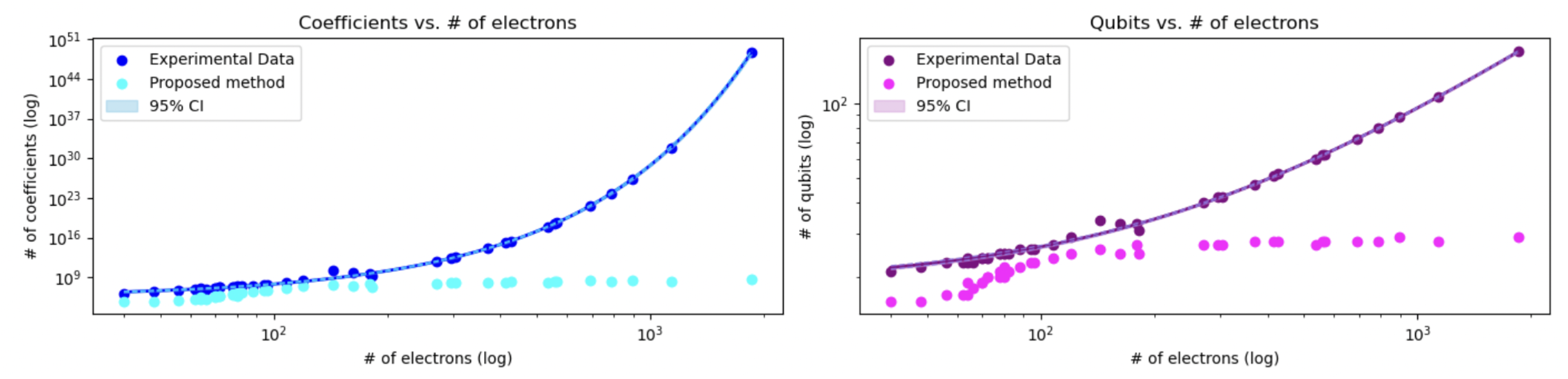
Our results demonstrate that fragmenting proteins into smaller units and reassembling them is an effective strategy for reducing the computational cost of quantum simulations. Key findings include:
- Scalability: The approach validated on small peptides extends to more complex systems such as Glucagon, maintaining controlled relative errors even for much bigger peptides (see Table 1).
- Resource Efficiency: The SelectSwap algorithm significantly reduces the number of Toffoli gates, albeit at the cost of a moderate increase in ancillary qubits. This trade-off is justified by the quadratic improvement in gate counts, which is crucial for scaling to larger systems.
- Predictive Models: Our regression models provide robust predictions of quantum resource requirements. The exponential model for coefficients achieved with stable confidence intervals, while the linear model for qubits performed consistently well, especially in medium-to-large systems. These models are reliable tools for early-stage quantum resource planning (see Table 3).
Relative errors of 2–3% observed for large systems (see Table 1), though higher than those for small peptides, remain within acceptable limits for many practical applications. For example, such tolerances are common in drug discovery workflows due to inherent experimental uncertainty.
Compared to classical fragmentation methods such as ONIOM, our approach achieves comparable or lower errors for small systems and holds the promise of exponential speedup for large-scale systems as quantum hardware matures. Furthermore, in contrast with other methodologies where the error tends to increase linearly with system size [12], our reported errors appear to stabilize when dealing with systems larger than approximately five amino acids.
Compared to MBE(n) methods, where the inclusion of higher-order n-body interactions comes with a significant computational, scaling scales approximately as [11], our strategy remains efficient. Moreover, while the inclusion of two-body interactions in MFCC-based schemes improves accuracy, it also increases computational demands due to the required calculations for fragment–fragment, fragment–cap, and cap–cap dimers [11].
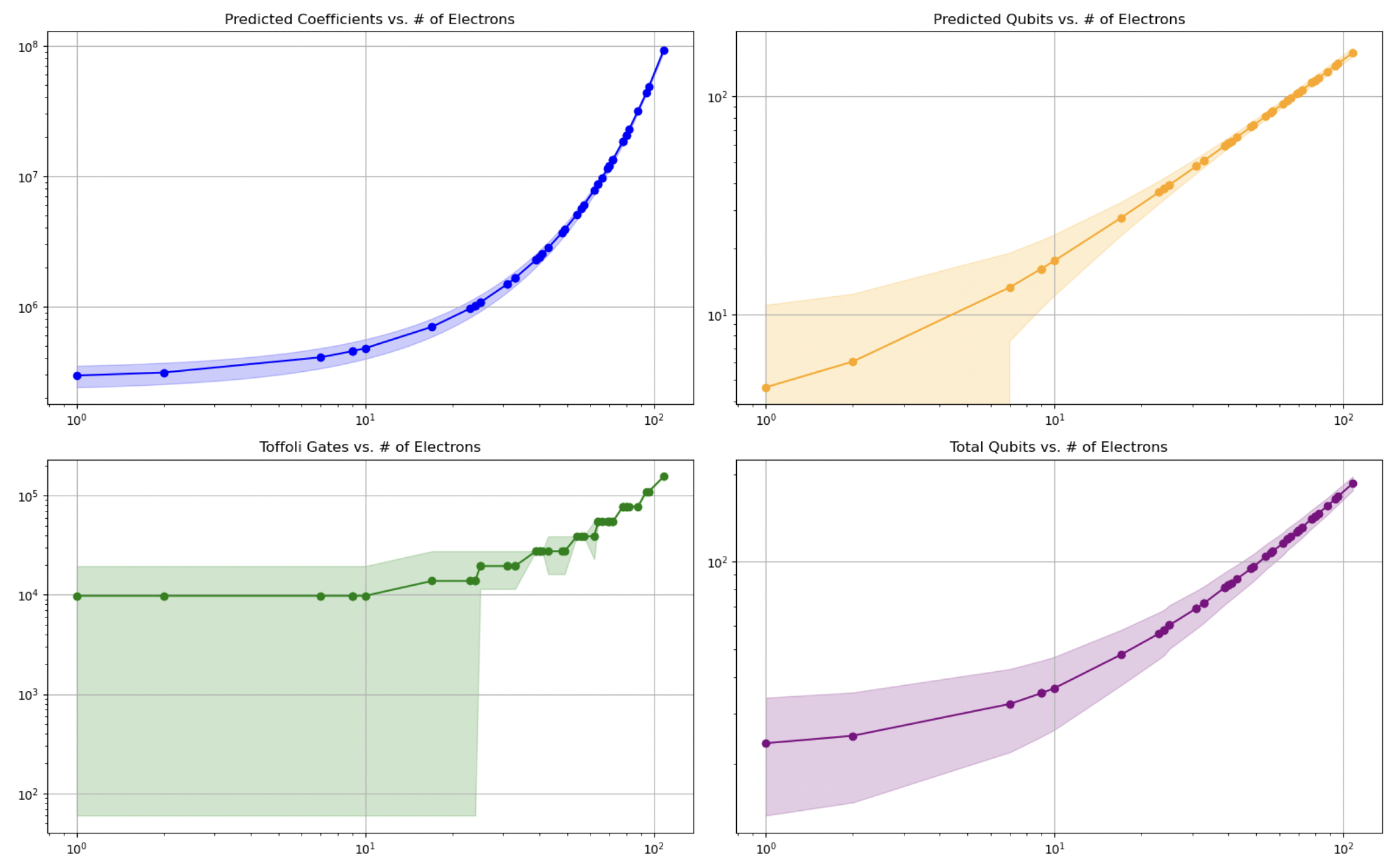
Figure 4.
Predicted quantum resource requirements as a function of the number of electrons. Top-left: exponential model of coefficient growth. Top-right: linear model for qubit requirements. Bottom-left: estimated Toffoli gate counts based on predicted coefficients. Bottom-right: total qubit requirements. Shaded regions indicate 95% confidence intervals. These trends support the scalability of the resource model across molecular sizes.
Therefore, our approach simplifies the fragmentation process, making it more attractive for hybrid quantum–classical schemes. Nevertheless, additional corrections may still be necessary, particularly for systems involving uncommon bonds or structural motifs. For such cases, our published dataset, QMProt [24], provides a foundation for studying post-chemical interaction corrections during the reassembly process. For example, we suspect that reducing the degree of fragmentation in such cases—e.g., by computing the energy of small groups of amino acids—could lead to even better results. This is in line with previous findings, which suggest that increased fragmentation may reduce accuracy [1].
A comparison with these studies also suggests that our strategy could be extended to other contexts, such as protein–protein or protein–ligand interactions. For instance, the human neurotensin peptide, which we also computed, could serve as a promising test case for our approach in protein-ligand scenarios, following the example set by [12].
With these advantages, our methodology opens new opportunities for accurately simulating peptides such as glucagon, enabling unprecedented insights into biological functions such as hormone signaling and enzyme catalysis, ultimately aiding drug development for diseases such as diabetes or cancer. Moreover, energy-based screening methods in drug discovery have been reported to be more efficient than distance-based ones [11].
A notable feature of our approach is that it introduces a form of computationally relative error—that is, the overall accuracy of the strategy is not rigidly defined by the model itself, but instead adapts to the computational precision of each fragment. As quantum algorithms and hardware evolve, the accuracy of each fragment-level simulation improves, and consequently, the total reassembled energy becomes increasingly precise. Unlike classical hybrid methods such as ONIOM, where the global error is bounded by structural approximations, our modular framework enables error reductions proportional to the quality of the underlying quantum simulation. This property positions the method as future-compatible and resilient to evolving quantum capabilities.
While our method demonstrates both scalability and accuracy across a range of system sizes, several limitations must be acknowledged. First, its applicability on real quantum hardware remains constrained by current noise and decoherence levels, with full advantages expected only in fault-tolerant regimes. Second, the reassembly process can introduce non-negligible errors, underscoring the need for chemically informed correction strategies. Finally, further integration of advanced techniques such as Quantum Phase Estimation (QPE), block encoding, and qubitization will be essential to enhance precision, though at the cost of increased circuit complexity. Overcoming these challenges is crucial for evolving the framework into a practical quantum simulation tool.
Alternative Hamiltonian reduction techniques such as symmetry tapering and active-space selection remain useful but limited:
- Global Symmetries: Typically eliminate 1–2 qubits per symmetry but are scarce in proteins.
- Point Group Symmetries: Allow deeper simplification but are difficult to apply globally to biomolecules.
In contrast, our approach applies symmetry detection fragment-wise, exploiting local structure—a more tractable and scalable strategy compatible with Intermediate-Scale Quantum (ISQ)-era devices and fault-tolerant systems alike.
This positions our methodology as a realistic bridge between the capabilities of the ISQ era [27] and the long-term quantum advantage in biochemical simulations.
6. Conclusions and Perspectives
This work presents a scalable and resource-efficient strategy for the quantum simulation of large protein systems, grounded in molecular fragmentation, regression-based resource estimation, and circuit optimization via the SelectSwap algorithm.
Our approach, initially validated on small peptides, has been successfully extended to more complex biomolecules such as Glucagon. Despite the increase in system size, the method maintains relative errors below 3% while significantly reducing computational overhead. In particular, the reduction in Toffoli gate counts—reaching up to 20 orders of magnitude—exemplifies the practical feasibility of simulating biologically relevant proteins within fault-tolerant architectures. The regression models employed not only provide reliable predictions of resource requirements but also enable pre-optimization of quantum workloads, thereby ensuring efficient deployment on current and future quantum hardware.
Looking ahead, several directions offer promising avenues for development. Expanding the molecular database will enhance the generalization and precision of regression models. Further integration of advanced quantum subroutines, such as Quantum Phase Estimation and state preparation techniques, is expected to refine energy accuracy, particularly in the chemical precision regime. It will also be essential to test the methodology on real quantum hardware to assess its robustness against noise and hardware constraints. Comparative studies with alternative strategies—such as tapering and active-space reduction—will help optimize the reassembly process, while the inherent modularity of the framework ensures that gains in quantum hardware performance directly translate into reductions in simulation error, without requiring reengineering of the underlying methodology.
Beyond its technical merits, this work contributes to the broader goal of enabling quantum advantage in computational biochemistry. The accurate simulation of large biomolecules remains a central challenge in drug discovery and protein engineering. By offering a path forward grounded in scalable design principles and resource-aware modeling, this framework lays the foundation for future breakthroughs in the quantum simulation of life sciences.
Appendix A. Source Code
The Python scripts used for model fitting, Toffoli gate estimation, and comparisons between full and fragmented simulations are publicly available at: github.com.
Appendix B. T–Gate Count from the Big–O Bound
We translate the Big–O bound from the reference [14] on the T–gate count into an explicit formula with constant factors. Specifically, the T–gate count required to implement the quantum lookup table is given by
where is the number of address qubits for a lookup table with N entries, and denotes the allowable error tolerance in the state preparation. The constants and depend on the gate decomposition and error-correction protocols [14].
This formula underpins the analysis in Section 3 and is directly used to estimate the quantum resource cost for each molecule (see Table 2).
The asymptotic bound is given by
which implies that for sufficiently large n and small , there exist constants such that
Our goal is to determine these constant factors explicitly.
Following the work developped in [14] (Sec. III, Fig. 8), the partition the memory into blocks of size is given by
so that the number of blocks is
Each block is processed via a quantum routing tree using non–Clifford operations (e.g., CSWAP or Toffoli gates). Let denote the T–gate cost per block, which includes the decomposition cost (e.g., a Toffoli gate typically decomposes into about 7 T–gates [14,28]) and an extra factor of due to error suppression. Hence, the T–gate cost per block is
Multiplying by the number of blocks in (A3), the primary query cost is
We set
Ancillary operations (uncomputing and error correction, e.g., via entanglement distillation [14]) contribute a cost proportional to . Let be the unit cost for these operations; then,
We define
Two key insights justify this formula:
The value of is influenced by the cost of decomposing complex non–Clifford operations. While a raw Toffoli gate might require approximately 7 T–gates [14,28], the unified architecture integrates several optimizations (e.g., reducing SWAP overhead, parallel processing, and gate cancellations) that lower the effective cost per block. Empirical and theoretical analyses in [14] and related literature (including [28,29,30]) support an effective value for in the range of 3 to 10. Similarly, reflects the cost of auxiliary operations for amplitude amplification and uncomputing. The procedure in [14] applies two such operations per query, each with a low, nearly constant T–gate cost (typically around 1 T–gate), leading to .
Appendix C. Regression Model Analysis for Coefficients and Qubits
This appendix presents a regression-based analysis to estimate the number of quantum coefficients and qubits from molecular electron count. Two techniques—Ordinary Least Squares (OLS) and RANSAC—were applied to assess model accuracy and robustness to outliers. Both linear and exponential forms were considered:
- Linear:
- Exponential:
Parameters a and b were obtained via least squares minimization, and predictions from the exponential model were back-transformed using .
Model performance was evaluated using standard metrics, notably the coefficient of determination , which quantifies the proportion of variance in the dependent variable explained by the independent variable. It is defined as:
To assess prediction accuracy, we computed the Mean Absolute Error (MAE) and the Root Mean Squared Error (RMSE). The MAE represents the average magnitude of the prediction errors, without considering their direction, and is given by Equation (A8):
The RMSE, in contrast, gives higher weight to larger errors due to the squaring of residuals, as defined in Equation (A9):
We also quantified the dispersion of the residuals using their standard deviation, as shown in Equation (A10):
Finally, the coefficient of variation (CV%) was calculated to express this variability relative to the mean predicted value, providing a normalized measure of dispersion. It is defined in Equation (A11):
In addition to point estimates, we computed 95% confidence intervals to characterize the uncertainty associated with the predictions. For the log-linear model of the coefficients, we first estimated the prediction using the exponential transformation , and then applied the delta method to propagate the uncertainty from the parameter estimates to the prediction.
This required computing the Jacobian vector of the model:
The variance of the predicted value was then calculated using the parameter covariance matrix, as in Equation (A13):
The resulting confidence interval for the prediction was obtained via:
For the linear model predicting the number of qubits, the confidence interval at a given input x was calculated using the standard error of the residuals and the classical formula for linear regression prediction intervals:
where s denotes the standard error of the residuals. These intervals are shown as shaded regions around the regression curves in the visualizations, providing a probabilistic interpretation of the expected variation in predicted values.
The analysis shows that while OLS provides a solid baseline, RANSAC enhances robustness, particularly for predicting quantum coefficients. For qubit estimation, both methods perform comparably, with RANSAC offering marginal gains. These regression models establish a reliable foundation for resource estimation, supporting scalability assessments and informing algorithmic and hardware design in quantum protein simulations.
References
- Sala, L.C.; Atchade-Adelemou, P. Efficient Protein Ground State Energy Computation via Fragmentation and Reassembly. arXiv 2025, arXiv:2501.03766. [Google Scholar]
- Atchade-Adelomou, P. Quantum algorithms for solving hard constrained optimisation problems. arXiv 2022, arXiv:2202.13125. [Google Scholar]
- Reiher, M.; Wiebe, N.; Svore, K.M.; Wecker, D.; Troyer, M. Elucidating reaction mechanisms on quantum computers. Proceedings of the national academy of sciences 2017, 114, 7555–7560. [Google Scholar] [CrossRef]
- Hohenberg, P.; Kohn, W. Density functional theory (DFT). Phys. Rev 1964, 136, B864. [Google Scholar] [CrossRef]
- Evangelisti, S.; Bendazzoli, G.L.; Gagliardi, L. Complete active-space configuration interaction with optimized orbitals: Application to Li2. International Journal of Quantum Chemistry 1995, 55, 277–280. [Google Scholar] [CrossRef]
- McArdle, S.; Endo, S.; Aspuru-Guzik, A.; Benjamin, S.C.; Yuan, X. Quantum computational chemistry. Reviews of Modern Physics 2020, 92, 015003. [Google Scholar] [CrossRef]
- Yang, P.J.; Sugiyama, M.; Tsuda, K.; Yanai, T. Artificial neural networks applied as molecular wave function solvers. Journal of Chemical Theory and Computation 2020, 16, 3513–3529. [Google Scholar] [CrossRef]
- Kitaura, K.; Ikeo, E.; Asada, T.; Nakano, T.; Uebayasi, M. Fragment Molecular Orbital Method: An Approximate Computational Method for Large Molecules. Chemical Physics Letters 1999, 313, 701–706. [Google Scholar] [CrossRef]
- Morokuma, M.; collaborators. ONIOM: a Multilayered Integrated MO + MM Method. Journal of Molecular Structure (THEOCHEM) 1999, 461–462, 1–21. [Google Scholar]
- ApSimon, J.; J. Bearpark, R. Adaptive QM/MM Methods for Chemical Reaction Dynamics. WIREs Computational Molecular Science 2023, 13, e1618. [Google Scholar]
- Bowling, P.E.; Broderick, D.R.; Herbert, J.M. Convergent Protocols for Computing Protein–Ligand Interaction Energies Using Fragment-Based Quantum Chemistry. Journal of Chemical Theory and Computation 2023, 19, 3656–3670. [Google Scholar] [CrossRef] [PubMed]
- Vornweg, J.R.; Wolter, M.; Jacob, C.R. A simple and consistent quantum-chemical fragmentation scheme for proteins that includes two-body contributions. Journal of Chemical Theory and Computation 2022, 18, 4516–4527. [Google Scholar] [CrossRef]
- Bravyi, S.; Gambetta, J.M.; Mezzacapo, A.; Temme, K. Tapering off qubits to simulate fermionic Hamiltonians, 2017, [arXiv:quant-ph/1701.08213].
- Zhu, S.; Sundaram, A.; Low, G.H. Unified architecture for a quantum lookup table. arXiv 2024, arXiv:2406.18030. [Google Scholar]
- Gosset, D.; Kothari, R.; Wu, K. Quantum state preparation with optimal T-count. arXiv 2024, arXiv:2411.04790. [Google Scholar]
- Carrera Vazquez, A.; Woerner, S. Efficient state preparation for quantum amplitude estimation. Physical Review Applied 2021, 15, 034027. [Google Scholar] [CrossRef]
- von Burg, V.; Low, G.H.; Häner, T.; Steiger, D.S.; Reiher, M.; Roetteler, M.; Troyer, M. Quantum computing enhanced computational catalysis. Physical Review Research 2021, 3. [Google Scholar] [CrossRef]
- Schollwöck, U. The density-matrix renormalization group. Reviews of modern physics 2005, 77, 259–315. [Google Scholar] [CrossRef]
- Perez-Garcia, D.; Verstraete, F.; Wolf, M.M.; Cirac, J.I. Matrix product state representations. arXiv preprint quant-ph/0608197 2006.
- Orús, R.; Mugel, S.; Lizaso, E. Tensor Networks for Complex Quantum Systems. Nature Reviews Physics 2019, 1, 538–550. [Google Scholar] [CrossRef]
- Chan, G.K.L.; Zgid, D. The Density Matrix Renormalization Group in Quantum Chemistry. Annual Reports in Computational Chemistry 2009, 5, 149–162. [Google Scholar] [CrossRef]
- Møller, C.; Plesset, M.S. Note on an Approximation Treatment for Many-Electron Systems. Physical Review 1934, 46, 618–622. [Google Scholar] [CrossRef]
- Xu, W.; coauthors. Adaptive Fragmentation Guided by Entanglement Metrics for Quantum Chemistry. arXiv 2025, arXiv:2502.12345. [Google Scholar]
- Sala, L.C.; Atchade-Adelomou, P. QMProt: A Comprehensive Dataset of Quantum Properties for Proteins. arXiv preprint arXiv:2505.08956 2025. Submitted on 13 May 2025.
- Hyndman, R.J.; Koehler, A.B. Another look at measures of forecast accuracy. International journal of forecasting 2006, 22, 679–688. [Google Scholar] [CrossRef]
- Low, G.H.; Kliuchnikov, V.; Schaeffer, L. Trading T gates for dirty qubits in state preparation and unitary synthesis. Quantum 2024, 8, 1375. [Google Scholar] [CrossRef]
- Atchade-Adelomou, P.; Gonzalez, S. Efficient quantum modular arithmetics for the isq era. arXiv 2023, arXiv:2311.08555. [Google Scholar]
- Amy, M.; Maslov, D.; Mosca, M.; Roetteler, M. A Meet-in-the-Middle Algorithm for Fast Synthesis of Depth-Optimal Quantum Circuits. IEEE Transactions on Computer-Aided Design of Integrated Circuits and Systems 2013, 32, 818–830. [Google Scholar] [CrossRef]
- Ross, N.J.; Selinger, P. Optimal ancilla-free Clifford+ T approximation of z-rotations. arXiv 2014, arXiv:1403.2975. [Google Scholar]
- Low, G.H.; Kliuchnikov, V.; Schaeffer, L. Trading T gates for dirty qubits in state preparation and unitary synthesis. Quantum 2024, 8, 1375. [Google Scholar] [CrossRef]
Figure 1.
Exponential fit of the total Hamiltonian coefficients () as a function of the number of electrons (). Blue markers represent data from QMProt [24], while the red curve corresponds to the fitted exponential model . The shaded area around the curve indicates the 95% confidence interval, capturing the uncertainty of the fit. This visualization highlights the exponential growth of coefficients with system size.
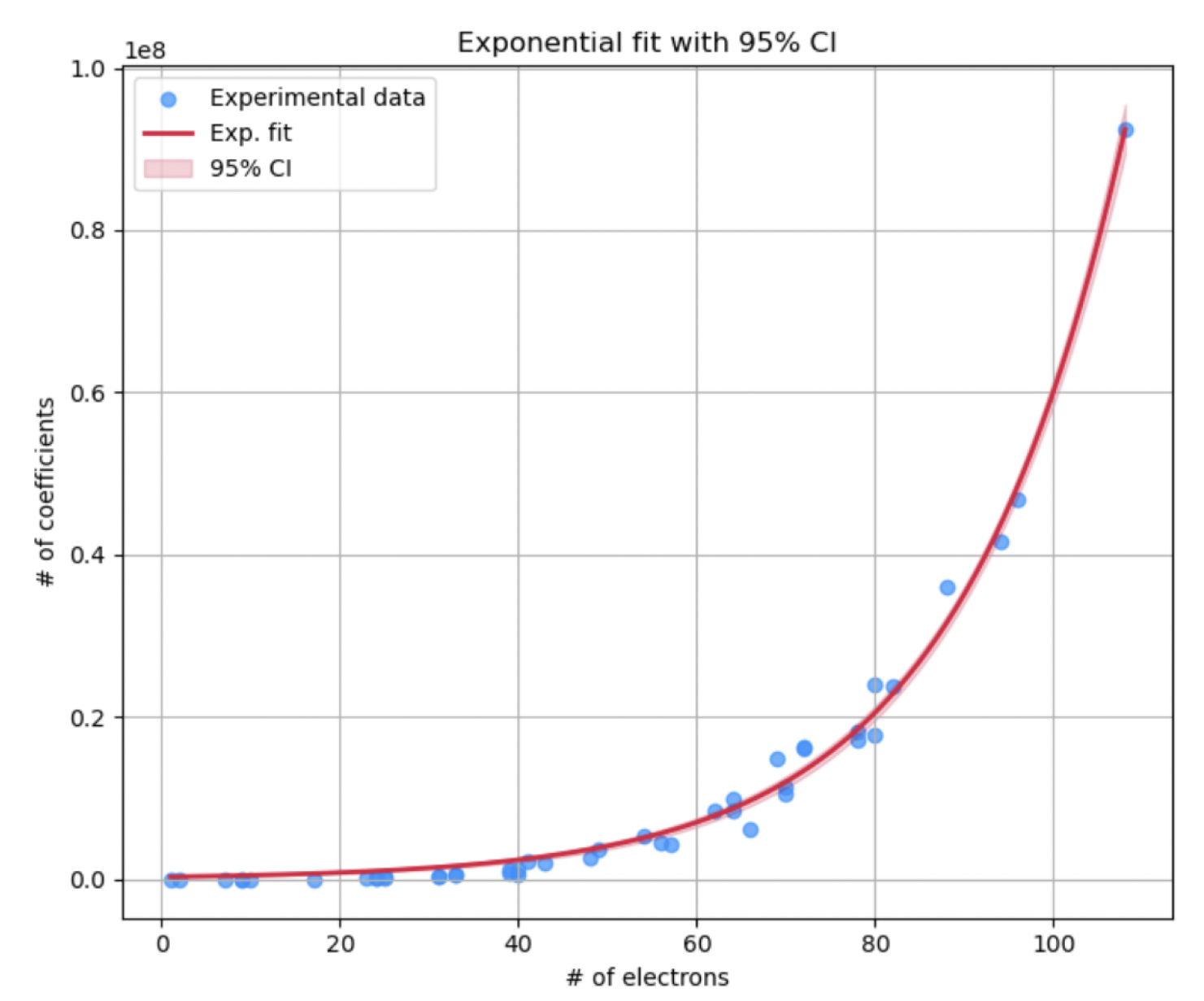
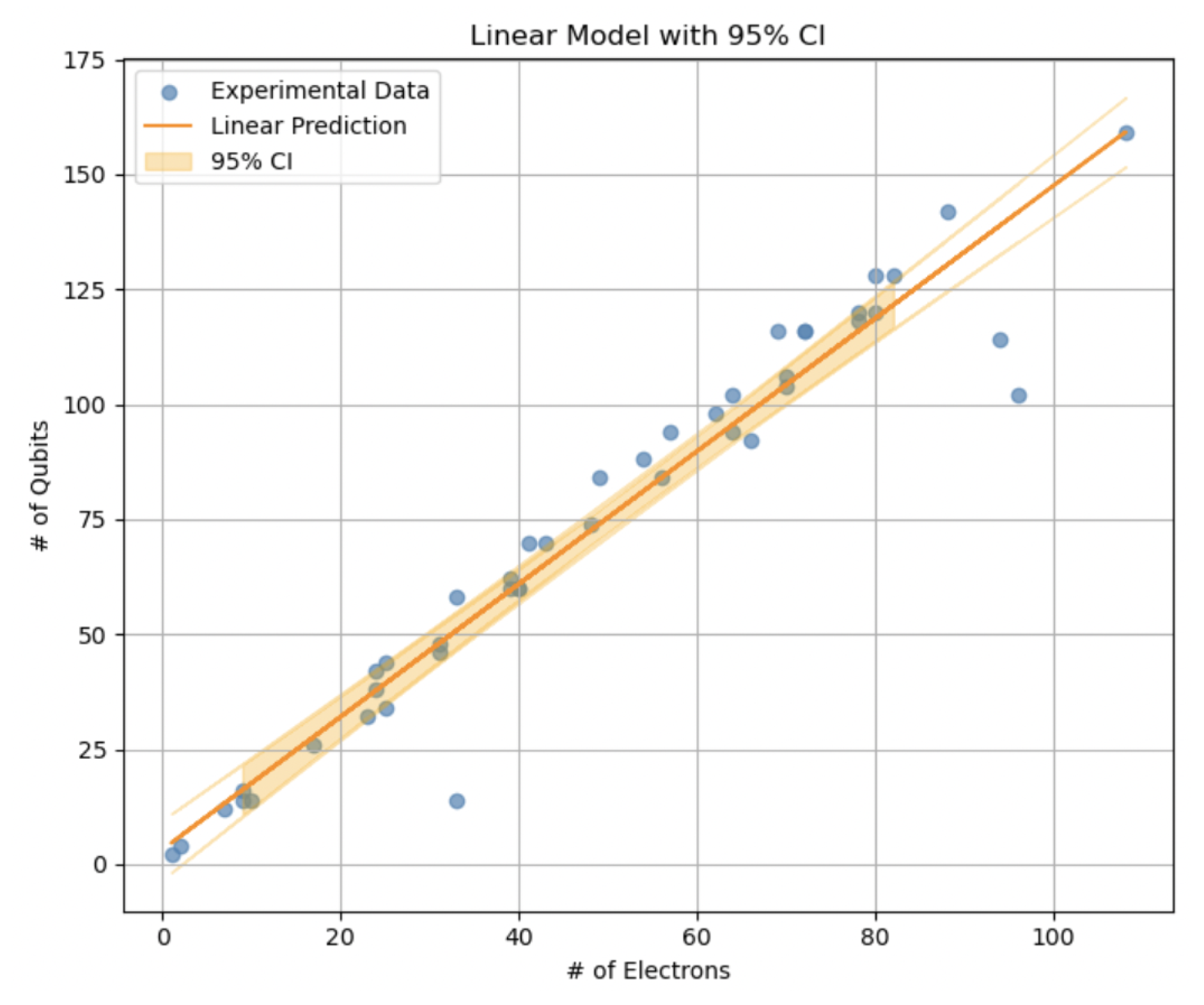
Figure 2.
Linear fit of the required qubits () as a function of the number of electrons (), using data from QMProt [24]. Blue markers denote empirical values, the orange line represents the fitted model , and the shaded band indicates the 95% confidence interval. The nearly linear relationship provides a useful estimate of qubit requirements as system size increases.
Disclaimer/Publisher’s Note: The statements, opinions and data contained in all publications are solely those of the individual author(s) and contributor(s) and not of MDPI and/or the editor(s). MDPI and/or the editor(s) disclaim responsibility for any injury to people or property resulting from any ideas, methods, instructions or products referred to in the content. |
© 2025 by the authors. Licensee MDPI, Basel, Switzerland. This article is an open access article distributed under the terms and conditions of the Creative Commons Attribution (CC BY) license (http://creativecommons.org/licenses/by/4.0/).
Copyright: This open access article is published under a Creative Commons CC BY 4.0 license, which permit the free download, distribution, and reuse, provided that the author and preprint are cited in any reuse.


