Existence and Uniqueness of the Viscous Burgers’ Equation Based on Ellis Model

1. Introduction

The classical Burgers’ equation ${\partial }_{t}u+u{\partial }_{x}u=\nu {\partial }_x^{2}u$ is a fundamental model in Newtonian fluid dynamics, often used to describe nonlinear wave propagation, turbulence and shock formation [1]. Its extension to non-Newtonian fluids is particularly significant in polymer science as these fluids exhibit complex viscosity behaviors that deviate from classical Newtonian assumptions. Non-Newtonian fluids, such as polymer solutions, colloidal suspensions, and biological substances, have viscosity that varies with the applied shear rate, requiring advanced models to accurately describe their flow characteristics [2]. Incorporating non-Newtonian properties into Burgers’ equation enables a more precise representation of fluid behavior, which is crucial for applications in industrial processes, biomedical engineering, and materials science. Some famous fluid problems for Burgers equation have been studied in [3,4,5,6,7]. Recent studies have explored some mathematical properties of Burgers’ equation with non-Newtonian viscosity, providing insight into the existence and stability of solutions for such models [8]. The author have recently studied the well-posedness of the initial-boundary value problem of the Burgers’ equation ${\partial }_{t}u+u{\partial }_{x}u=\nu {\partial }_x\left(|{\partial }_x{u|}^{p-2}{\partial }_{x}u\right)$ for power-law fluids in [9].

Ellis rheological model effectively captures shear-thinning effects, where viscosity decreases as shear rate increases, a phenomenon commonly observed in polymeric and biological fluids. Ellis law in rheology literature can be given by the equation $\dot{\gamma }={\displaystyle \frac{1}{{\mu }_0}}\left[1+{\left|{\displaystyle \frac{\tau }{{\tau }_{1/2}}}\right|}^{\alpha -1}\right]\tau$, in which $\dot{\gamma }={\partial }_{x}u$ is shear rate along x, and $\tau$ is the shear stress, typically measured in rotational rheometers, ${\mu }_0$ is the zero-shear viscosity, $\alpha$ is the measure of shear-thinning behavior ($\alpha >1$ is shear-thinning), ${\tau }_{1/2}$ is the shear stress at which the apparent viscosity has dropped to half its zero-shear viscosity value [10].It is a widely used mathematical model by engineers, see, e.g., [11,12,13]. The Burgers’ equation can be derived from the Navier-Stokes equation [14] for Ellis’ law by dropping the pressure gradient, gravitational, external forces, and the incompressible condition, which takes the form ${\partial }_{t}u+u{\partial }_{x}u=\nu {\partial }_x\left({\varphi }^{-1}\left({\partial }_{x}u\right)\right)$. This equation can be used to model stationary fluid between parallel plates subject to a sudden move with an initiate velocity. Although it is a greatly simplified the Navier-Stokes equations, by studying it mathematically allows for a deeper understanding of shear-thinning fluid dynamics. This study aims to establish rigorous well-posedness for Burgers’ equation based on the Ellis rheology model, contributing to a deeper understanding of non-Newtonian fluid mechanics and its engineering and scientific applications. While previous research has explored the mathematical framework of Burgers’ equation with non-Newtonian viscosity [7,15], open questions remain regarding the existence, uniqueness and stability of solutions. For this purpose we study the well-posedness and numerical solutions of the Burgers’ equation based on Ellis law with initial and boundary conditions:

$$\left\{\begin{array}{cc}{\partial }_{t}u+u{\partial }_{x}u=\nu {\partial }_x\left({\varphi }^{-1}\left({\partial }_{x}u\right)\right),\hfill & x\in [0,l],t\in [0,T],\hfill \\ u(0,x)=u_0\left(x\right),\hfill & x\in [0,l],\hfill \\ u(t,0)=u(t,l)=0,\hfill & t\in [0,T].\hfill \end{array}\right.$$

(1)

In the following we will prove the result concerning the existence and uniqueness of a solution to Problem (1) in the Bochner space $L^2\left(0,T;{W_0}^{1,p}(0,l)\right)$, where $p=1+{\displaystyle \frac{1}{\alpha }}$. For definitions and descriptions of the Bochner spaces with application for parabolic and hyperbolic PDEs, see, e.g., [16]. In contrast to the Burgers’ problems for power law fluids studies in [9], the Burgers’ problem (1) is technically more challenging, due to the fact that the function ${\varphi }^{-1}\left(\tau \right)$ has no explicit algebraic expression, and for this we derive lower and upper bounds for the inverse function (see Proposition 6 in Section 2) to allow analysis in proving the existence and uniqueness of solution to the problem.

Multiplying the equation of (1) by a test function $w\in W_0^{1,p}(0,l)$ and integrating formally by parts from 0 to l, we convert the initial-boundary value problem (1) to the following integral identity

$${\int }_0^l{\partial }_{t}uwdx+{\int }_0^{l}u{\partial }_{x}uwdx+\nu {\int }_0^l{\varphi }^{-1}\left({\partial }_{x}u\right){\partial }_{x}wdx=0$$

(2)

for all $w\in W_0^{1,p}(0,l)$ with $p=1+{\displaystyle \frac{1}{\alpha }}$, $t\in (0,T)$.

Definition 1.

A function $u\in L^2\left(0,T;{W_0}^{1,p}(0,l)\right)$ for which ${\partial }_{t}u\in$$L^2\left(0,T;L^2(0,l)\right)$ is said to be a weak solution of problem (1) if it satisfies (2) for each $w\in {W_0}^{1,p}(0,l)$ and a.e. $t\in (0,T)$ and $u(0,x)=u_0$ for all $x\in (0,l)$, $p>1$ with $p=1+{\displaystyle \frac{1}{\alpha }}$.

The main result of this work is gathered in the following theorem on the existence and uniqueness of the solution for initial-boundary value (1).

Theorem 1.

Let $u_0\in W_0^{1,p}(0,l)$ with $p=1+{\displaystyle \frac{1}{\alpha }}$. Then there exists a unique solution $u\in L^2\left(0,T;{W_0}^{1,p}(0,l)\right)$ of (1) such that ${\partial }_{t}u\in L^2\left(0,T;L^2(0,l)\right)$ in the sense of Definition 1.

In Section 2, we state some preliminary information needed to study the well-posedness of the problem (1), formulated in the weak form (2). Section 3 consists of two subsection 3.1 and subsection 3.2. We obtain the existence result in Section 3.1 and establish the uniqueness of the solution in Section 3.2. Moreover, in Section 4, we construct the numerical solutions using the COMSOL PDE solver with some numerical manipulations.

2. Preliminary

It is well known that $L^p(0,l)$ and $W^{k,p}(0,l)$ are the standard spaces of Lebesgue and Sobolev, respectively, for $1<p<\infty$ and $k\in \mathbb{Z}$. For any Banach space X, we define $L^p(0,T;X)$ to be the space of measurable functions $u:(0,T)\to X$ such that

$${\parallel u\parallel }_{L^p(0,T;X)}={\left({\int }_0^T{\parallel u\parallel }_X^p\mathrm{d}t\right)}^{1/p}<\infty$$

for $1<p<\infty$ and ${\parallel u\parallel }_{L^{\infty }(0,T;X)}=ess{sup}_{0<t<T}{\parallel u\parallel }_X<\infty$ if $p=\infty$. $L^p(0,T;X)$ is a Banach space [17]. The Sobolev space $W^{1,p}(0,1)$ consists of functions whose weak derivatives are integrable in $L^p(0,1)$.

$〈·,·〉$ denotes the inner product of two vectors in $L^2(0,1)$; that is,

$$〈f,g〉={\int }_0^{1}f\overline{g}dx.$$

In the following, we present several propositions that are well-established theorems in the literature, which will be used in Section 3.

Proposition 1

(Jensen’s inequality [18]). Let $(\Omega ,\Lambda ,\mu )$ be a measure space with $0<\mu (\Omega )<\infty$ and let $\phi :I\to \mathbb{R}$ be a convex function defined on an open interval I in $\mathbb{R}$ if $f:\Omega \to I$ is such that $f,\phi \circ f\in L(\Omega ,\Lambda ,\mu )$, then

$$\phi \left({\displaystyle \frac{1}{\mu (\Omega )}}{\int }_{\Omega }fd\mu \right)\le {\displaystyle \frac{1}{\mu (\Omega )}}{\int }_{\Omega }\phi \left(f\right)d\mu .$$

Proposition 2

(Aubin–Lions lemma [19]). Let $X_0,X$ and $X_1$ be three Banach spaces with $X_0\subseteq X\subseteq X_1$. Suppose that $X_0$ is compactly embedded in X and that X is continuously embedded in $X_1$. For $1\le p,q\le \infty$, let

$$W=\left\{u\in L^p\left([0,T];X_0\right)\mid \dot{u}\in L^q\left([0,T];X_1\right)\right\}.$$

(i) 

If $p<\infty$, then the embedding of W into $L^p([0,T];X)$ is compact.

(ii) 

If $p=\infty$ and $q>1$, then the embedding of W into $C\left(\right[0,T];X)$ is compact.

Proposition 3

(Rellich-Kondrachov Compactness Theorem [20]). Assume U is a bounded open subset of ${\mathbb{R}}^n$ and $\partial U$ is $C^1$. Suppose $1\le p<n$. Then

$$W^{1,p}\left(U\right)\subset \subset L^q\left(U\right)$$

for each $1\le q<p^{*}$.

Proposition 4

([21]). If f is a Lebesgue measurable function defined on a closed, bounded interval [a,b], with its $L^p$ norm for $1<p<\infty$ defined by

$${\parallel f\parallel }_p={\left({\int }_a^b{\left|f\left(x\right)\right|}^{p}dx\right)}^{1/p}$$

and $L^{\infty }$ norm

$${\parallel f\parallel }_{\infty }=\mathrm{ess}.\sup .\left\{\right|f\left(x\right)|:a\leqq x\leqq b\}.$$

If $f_1,f_2,f_3,\dots$ is a sequence of measurable functions and M is a positive constant such that

$${∥f_n∥}_{\infty }\leqq Mn=1,2,\dots$$

and ${lim}_{n\to \infty }{f}_n\left(x\right)=f\left(x\right)$ a.e. $x\in [a,b]$, then

$$\underset{n\to \infty }{lim}{∥f_n-f∥}_p=0$$

for any p satisfying $0<p<\infty$.

Proposition 5

(The differential form of Gronwall’s inequality [20]).

(i) 

Let $\eta (·)$ be a nonnegative, absolutely continuous function on $[0,T]$, which satisfies for a.e. t the differential inequality

$${\eta }^{\prime }\left(t\right)\le \varphi \left(t\right)\eta \left(t\right)+\psi \left(t\right),$$

where $\varphi \left(t\right)$ and $\psi \left(t\right)$ are nonnegative summable functions on $[0,T]$. Then

$$\eta \left(t\right)\le e^{{\int }_0^t\varphi \left(s\right)ds}\left[\eta \left(0\right)+{\int }_0^t\psi \left(s\right)ds\right]$$

for all $0\le t\le T$.

(ii) 

In particular, if

$${\eta }^{\prime }\le \varphi \eta \mathrm{on}[0,T]\mathrm{and}\eta \left(0\right)=0,$$

then

$$\eta \equiv 0\mathrm{on}[0,T].$$

We first introduce the lower bound for the inverse function of $\varphi$ in Ellis law.

Proposition 6.

Let $t=\varphi \left(\tau \right)=\tau (1+c|\tau {|}^{\alpha })$, $\alpha >0$ and let $\tau ={\varphi }^{-1}\left(t\right)$ be the inverse function. Then${\left[{\varphi }^{-1}\left(t\right)\right]}^{\prime }={\displaystyle \frac{1}{1+{(\alpha +1)c\left|\tau \right|}^{\alpha }}}$ and

$${\varphi }^{-1}\left(t\right)t⩾\left\{\begin{array}{cc}{c}_1{t}^2\hfill & for0⩽t<1,\hfill \\ c_2{\left|t\right|}^{1+{\displaystyle \frac{1}{\alpha }}}\hfill & fort⩾1,\hfill \end{array}\right.$$

(3)

where $c_1={\displaystyle \frac{1}{1+c}}$ and $c_2={\displaystyle \frac{1}{{|1+c|}^{\frac{1}{\alpha }}}}$ are constant numbers.

Proof. 

It is obvious that

$$\varphi \le \left\{\begin{array}{cc}(1+c)\tau \hfill & \mathrm{for}\tau <1,\hfill \\ {(1+c)\left|\tau \right|}^{\alpha }\tau \hfill & \mathrm{for}\tau ⩾1.\hfill \end{array}\right.$$

Therefore, for the inverse function the following inequality

$${\varphi }^{-1}\left(t\right)⩾\left\{\begin{array}{cc}{\displaystyle \frac{1}{1+c}}t\hfill & \mathrm{for}c⩽t<1+c,\hfill \\ {\left|{\displaystyle \frac{1}{1+c}}t\right|}^{{\displaystyle \frac{1}{\alpha }}-1}t\hfill & \mathrm{for}1+c⩽t\hfill \end{array}\right.$$

(4)

holds.

The multiplication of both sides of the previous inequalities by t leads us to

$${\varphi }^{-1}\left(t\right)t⩾\left\{\begin{array}{cc}{\displaystyle \frac{1}{1+c}}{t}^2\hfill & \mathrm{for}c⩽t<1+c,\hfill \\ {\left|{\displaystyle \frac{1}{1+c}}\right|}^{{\displaystyle \frac{1}{\alpha }}}{\left|t\right|}^{1+{\displaystyle \frac{1}{\alpha }}}\hfill & \mathrm{for}1+c⩽t.\hfill \end{array}\right.$$

We split the domain of definition of function in the following way

$${\varphi }^{-1}\left(t\right)t⩾\left\{\begin{array}{cc}{\displaystyle \frac{1}{1+c}}{t}^2\hfill & \mathrm{for}c⩽t<1,\hfill \\ {\displaystyle \frac{1}{1+c}}{t}^2\hfill & \mathrm{for}1⩽t<1+c,\hfill \\ {\displaystyle \frac{1}{{|1+c|}^{\frac{1}{\alpha }}}}{\left|t\right|}^{1+{\displaystyle \frac{1}{\alpha }}}\hfill & \mathrm{for}1+c⩽t<\infty .\hfill \end{array}\right.$$

Further, decreasing the lower bound of ${\varphi }^{-1}\left(t\right)t$ gives

$${\varphi }^{-1}\left(t\right)t⩾\left\{\begin{array}{cc}{\displaystyle \frac{1}{1+c}}{t}^2\hfill & \mathrm{for}0⩽t<1,\hfill \\ {\displaystyle \frac{1}{1+c}}{\left|t\right|}^{1+{\displaystyle \frac{1}{\alpha }}}\hfill & \mathrm{for}1⩽t<1+c,\hfill \\ {\displaystyle \frac{1}{{|1+c|}^{\frac{1}{\alpha }}}}{\left|t\right|}^{1+{\displaystyle \frac{1}{\alpha }}}\hfill & \mathrm{for}1+c⩽t<\infty .\hfill \end{array}\right.$$

Finally, we get

$${\varphi }^{-1}\left(t\right)t⩾\left\{\begin{array}{cc}{c}_1{t}^2\hfill & \mathrm{for}0⩽t<1,\hfill \\ c_2{\left|t\right|}^{1+{\displaystyle \frac{1}{\alpha }}}\hfill & \mathrm{for}t⩾1,\hfill \end{array}\right.$$

where $c_1={\displaystyle \frac{1}{1+c}}$ and $c_2={\displaystyle \frac{1}{{|1+c|}^{\frac{1}{\alpha }}}}$.

So, the proof of this proposition is complete. We will prove the existence and uniqueness of the solution in the next Section 3. □

3. Existence and Uniqueness

In this section, we prove two theorems and some auxiliary lemmas, which we invoke to establish the existence and uniqueness result for the viscous Burgers’ equation for the isothermal flow of Ellis fluids with initial and boundary conditions.

3.1. Existence

In this subsection, we will prove the existence of solutions to the problem formulated in the integral equation (2). Firstly, we choose the basis ${\left\{e_i\right\}}_{j\in \mathbb{N}}\in L^2(0,l)$ defined as a subset of the eigenfunction of the Laplacian for the Dirichlet problem

$$\left\{\begin{array}{c}-{\partial }_x^2{e}_j={\lambda }_j{e}_j,j\in \mathbb{N},\\ e_j=0,x\in \{0,l\},\end{array}\right.$$

(5)

where

$$e_j=sin{\displaystyle \frac{j\pi }{l}}x,{\lambda }_j={\left({\displaystyle \frac{j\pi }{l}}\right)}^2$$

(6)

for $j\in \mathbb{N}$. It’s known that ${\left\{e_j\right\}}_{j\in N}$ is an orthonormal basis in $L^2(0,l)$. Then for $f\in L^2(0,l)$, we can write

$$f=\sum _{j=1}^{\infty }{c}_j\left(t\right)e_j$$

with $c_j\left(t\right)={\left({\int }_0^l{\left|f{e}_j\right|}^{2}dx\right)}^{1/2}<\infty ,j=1,2,\dots$ and the sequence ${\left\{c_j\right\}}_1^{\infty }$ is converges uniformly in $L^{\infty }(0,T;l^2)$.

Then, we introduce the approximate solution $u_n(t,x)$ by

$$u_n(t,x)=\sum _{j=1}^n{c}_j\left(t\right)e_j,$$

(7)

$$u_n\left(0\right)=u_{0n}=\sum _{j=1}^n{c}_j\left(0\right)e_j$$

(8)

which has to satisfy the approximate problem

$${\int }_0^l{\partial }_t{u}_n{e}_{j}dx+{\int }_0^l{u}_n{\partial }_x{u}_n{e}_{j}dx+\nu {\int }_0^l{\varphi }^{-1}\left({\partial }_x{u}_n\right){\partial }_x{e}_{j}dx=0,$$

(9)

$$u_n\left(0\right)=u_{0n}$$

for all $j=1,\dots ,n$ , $t\in [0,T]$.

Remark 1.

The coefficients $c_j\left(0\right)$ can be chosen such that ${lim}_{n\to \infty }{u}_{0n}=u\left(0\right)$ in $W_0^{1,1+{\displaystyle \frac{1}{\alpha }}}(0,l)$.

Furthermore, we prove the lemma concerning the solution of approximate problem (9).

Lemma 1.

If ϕ is the function specified in Proposition 6. Then the inverse function ${\varphi }^{-1}$ satisfies the following inequality

$${\int }_0^l{\varphi }^{-1}\left(u_{nx}\right)u_{nx}dx⩾c_1\parallel u_{nx}{\parallel }_{L^{1+{\displaystyle \frac{1}{\alpha }}}(0,l)}^2+c_2{\parallel u_{nx}\parallel }_{L^{1+{\displaystyle \frac{1}{\alpha }}}(0,l)}^{1+{\displaystyle \frac{1}{\alpha }}},$$

where $c_1$, $c_2$ and $\alpha >0$ are constants from Proposition 6.

Proof. 

Integration inequality (3) from 0 to 1 gives

$$\begin{array}{cc}\hfill {\int }_0^l{\varphi }^{-1}\left(u_{nx}\right)u_{nx}dx& ={\int }_{A=\left\{x:\left|u_{nx}\right|⩾1\right\}}{\varphi }^{-1}\left(u_{nx}\right)u_{nx}dx+{\int }_{B=\left\{x:\left|u_{nx}\right|\le 1\right\}}{\varphi }^{-1}\left(u_{nx})u_{nx}dx\right.\hfill \\ \hfill & ⩾c_2{\int }_A{\left|u_{nx}\right|}^{1+{\displaystyle \frac{1}{\alpha }}}dx+c_1{\int }_B{\left|u_{nx}\right|}^{2}dx.\hfill \end{array}$$

(10)

Application the Jensen’s inequality (see Proposition 1) to the last term on the right-hand side of inequality (10) leads us

$${\left[{\int }_B{c}_1{\left|u_{nx}\right|}^{2}dx\right]}^{{\displaystyle \frac{1+\frac{1}{\alpha }}{2}}}⩾c_1\left[{\int }_B{\left|u_{nx}\right|}^{1+{\displaystyle \frac{1}{\alpha }}}dx\right]=c_1{\parallel u_{nx}\parallel }_{L^{1+{\displaystyle \frac{1}{\alpha }}}(0,l)}^2.$$

Consequently, using the last inequality to (10), we obtain the desirable estimate

$${\int }_0^l{\varphi }^{-1}\left(u_{nx}\right)u_{nx}dx⩾c_1\parallel u_{nx}{\parallel }_{L^{1+{\displaystyle \frac{1}{\alpha }}}(0,l)}^2+c_2{\parallel u_{nx}\parallel }_{L^{1+{\displaystyle \frac{1}{\alpha }}}(0,l)}^{1+{\displaystyle \frac{1}{\alpha }}}$$

with $c_1$ and $c_2$ from Proposition 6. The proof of the lemma is complete. □

Theorem 2.

There exists a positive constant $C_0>0$ independent on n, that satisfies the following inequality

$${∥u_n∥}_{L^2(0,l)}^2+{\int }_0^t\left(C_1\parallel u_{nx}{\parallel }_{L^{1+{\displaystyle \frac{1}{\alpha }}}(0,l)}^2+C_2{\parallel u_{nx}\parallel }_{L^{1+{\displaystyle \frac{1}{\alpha }}}(0,l)}^{1+{\displaystyle \frac{1}{\alpha }}}\right)d\tau ⩽C_0$$

for all $t\in [0,T]$.

Proof. 

Taking $e_j=u_n$ in (9), we obtain

$${\int }_0^l{u}_n{\partial }_t{u}_{n}dx+{\int }_0^l{u}_n^2{\partial }_x{u}_{n}dx+\nu {\int }_0^l{\varphi }^{-1}\left({\partial }_x{u}_n\right){\partial }_x{u}_{n}dx=0.$$

(11)

The first term of (11) can be written as follows

$${\int }_0^l{u}_n{\partial }_t{u}_{n}dx={\displaystyle \frac{1}{2}}{\displaystyle \frac{d}{dt}}{\int }_0^l{u}_n^{2}dx={\displaystyle \frac{1}{2}}{\displaystyle \frac{d}{dt}}{∥u_n∥}_{L^2(0,l)}^2.$$

(12)

Computing the second integral of (11) by the initial condition in (9) leads us to

$${\int }_0^l{u}_n^2{\partial }_x{u}_{n}dx={\int }_0^l{\partial }_x\left(u_n^3\right)dx={\left.u_n^3\right|}_0^l=0.$$

(13)

By substituting the integrals (12) and (13) into (11) and integrating the equation (11) from 0 to t with respect to $\tau$, we have

$${∥u_n∥}_{L^2(0,l)}^2+\nu {\int }_0^t{\int }_0^l{\varphi }^{-1}\left({\partial }_x{u}_n\left(\tau \right)\right){\partial }_x{u}_n\left(\tau \right)dxd\tau ={∥u_{n0}∥}_{L^2(0,l)}^2.$$

Application of inequality in Proposition 6 to the second term on the left-hand side of the last equation leads us

$${∥u_n∥}_{L^2(0,l)}^2+{\int }_0^t\left(C_1\parallel u_{nx}{\parallel }_{L^{1+{\displaystyle \frac{1}{\alpha }}}(0,l)}^2+C_2{\parallel u_{nx}\parallel }_{L^{1+{\displaystyle \frac{1}{\alpha }}}(0,l)}^{1+{\displaystyle \frac{1}{\alpha }}}\right)d\tau ⩽C_0$$

with $C_0={∥u_{n0}∥}_{L^2(0,l)}^2$.

The proof of the theorem is complete. □

Theorem 3.

For each $n\in {\mathbb{N}}^{+}$ problem (9) has at least one solution $u_n,{\displaystyle \frac{\partial u_n}{\partial t}}\in L^2(0,T;W_0^{1,1+{\displaystyle \frac{1}{\alpha }}}(0,l))$.

Proof. 

Now we represent the approximate equation (9) in the following form

$${\int }_0^l{\displaystyle \frac{\partial u_n}{\partial t}}{e}_{j}dx=-{\int }_0^l{u}_n{\partial }_x{u}_n{e}_{j}dx-\nu {\int }_0^l{\varphi }^{-1}\left({\partial }_x{u}_n\right){\partial }_x{e}_{j}dx$$

(14)

for $j=1,\dots ,n$. The integral on the left-hand side of (14) can be written as below

$${\int }_0^l{\displaystyle \frac{\partial u_n}{\partial t}}{e}_{j}dx={\int }_0^l\sum _{i=1}^n{\dot{c}}_i\left(t\right)e_i{e}_{j}dx={\dot{c}}_j\left(t\right),j=1,\dots ,n.$$

(15)

First integral on the right-hand side of (14) is equal to zero

$$\begin{array}{cc}\hfill {\int }_0^l{u}_n{\partial }_x{u}_n{e}_{j}dx& ={\int }_0^l\left(\sum _{i=1}^n{c}_i\left(t\right)e_i\right)\left(\sum _{k=1}^n{c}_k\left(t\right)e_k^{\prime }\right)e_{j}dx\hfill \\ \hfill & =\sum _{i=1}^n\sum _{k=1}^n{c}_i\left(t\right)c_k\left(t\right){\int }_0^l{e}_i\left(x\right)e_j\left(x\right)e_k^{\prime }\left(x\right)dx=0\hfill \end{array}$$

(16)

for $j=1,\dots ,n$, since

$${\int }_0^l{e}_i\left(x\right)e_j\left(x\right)e_k^{\prime }\left(x\right)dx=0,i,j,k=1,\dots ,n.$$

(17)

We show (17). By (6), we note that

$$e_i\left(x\right)e_j\left(x\right)e_k^{\prime }\left(x\right)={\displaystyle \frac{k\pi }{l}}sin{\displaystyle \frac{i\pi }{l}}xsin{\displaystyle \frac{j\pi }{l}}xcos{\displaystyle \frac{k\pi }{l}}xi,j,k=1,\dots ,n.$$

Then, by well-known formula 402.05 [Dwight]

$$4sinAsinBcosC=-cos(A+B-C)+cos(B+C-A)+cos(A+C-B)-cos(A+B+C),$$

(18)

we obtain (17).

Thus, substitutions of (15) and (16) into (14) lead us to the following linear ordinary system of n equations with respect to t

$${\dot{c}}_j\left(t\right)=-\nu {\int }_0^l{\varphi }^{-1}(\sum _{i=1}^n{c}_i\left(t\right)e_i^{\prime })e_j^{\prime }dx$$

(19)

for $j=1,\dots ,n$.

Now we introduce the following notations:

$$\overrightarrow{b}:=\nu {\int }_0^l{\varphi }^{-1}(\overrightarrow{c}·{\overrightarrow{e}}^{\prime })\overrightarrow{e}dx,$$

where

$$\begin{array}{cc}& \overrightarrow{c}\left(t\right)=\left(\begin{array}{c}{c}_1\left(t\right)\\ c_2\left(t\right)\\ ⋮\\ c_n\left(t\right)\end{array}\right),\overrightarrow{b}=\left(\begin{array}{c}\nu {\int }_0^l{\varphi }^{-1}\left(\sum _{i=1}^n{c}_i\left(t\right)e_i^{\prime }\right)e_1^{\prime }dx\\ \nu {\int }_0^l{\varphi }^{-1}\left(\sum _{i=1}^n{c}_i\left(t\right)e_i^{\prime }\right)e_2^{\prime }dx\\ ⋮\\ \nu {\int }_0^l{\varphi }^{-1}\left(\sum _{i=1}^n{c}_i\left(t\right)e_i^{\prime }\right)e_n^{\prime }dx\end{array}\right).\hfill \end{array}$$

Hence, we rewrite system (19) as follows

$$\dot{\overrightarrow{c}}=-\overrightarrow{b}\left(\overrightarrow{c}\right).$$

(20)

So, ${\varphi }^{-1}$ in the term $\overrightarrow{b}\left(\overrightarrow{c}\right)$ satisfies the Lipschitz condition by Proposition 6. Therefore, the system (20) has a solution $\overrightarrow{c}\left(t\right)=(c_1\left(t\right),c_2\left(t\right),\dots ,c_n\left(t\right))$ by the Existence Theorem for the ODE system. □

We are now ready to prove the following theorem.

Theorem 4.

There exists a weak solution of the problem (2) such that $u,u_t\in L^2(0,T;W_0^{1,1+{\displaystyle \frac{1}{\alpha }}}(0,l))$.

Proof. 

By Theorem 3 there exists a weak solution $u_n$ of the approximating problem (9) in $L^2(0,T;W_0^{1,1+{\displaystyle \frac{1}{\alpha }}}(0,l))$. We take $W=\{{\left\{u_n\right\}}_{n=1}^{\infty }\in L^2(0,T;W_0^{1,1+{\displaystyle \frac{1}{\alpha }}}(0,l))|{\left\{{\partial }_t{u}_n\right\}}_{n=1}^{\infty }\in L^2(0,T;W_0^{1,1+{\displaystyle \frac{1}{\alpha }}}(0,l))\}$. We note that ${\left\{u_n\right\}}_{n=1}^{\infty }\in L^2(0,T;W_0^{1,1+{\displaystyle \frac{1}{\alpha }}}(0,l))$ by our construction in subsection 3.1. By Theorem 2, the sequence ${\left\{u_n\right\}}_{n=1}^{\infty }$ is bounded in $L^2(0,T;W_0^{1,1+{\displaystyle \frac{1}{\alpha }}}(0,l))$.

Now we show that ${\left\{{\partial }_t{u}_n\right\}}_{n=1}^{\infty }\in L^2(0,T;W_0^{1,1+{\displaystyle \frac{1}{\alpha }}}(0,l))$. Equation (7) implies that

$${\partial }_t{u}_n(t,x)=\sum _{j=1}^n{\dot{c}}_j\left(t\right)e_j.$$

Therefore,

$$\parallel {\partial }_t{u}_n{\parallel }_{L^2(0,l)}^2=\langle {\partial }_t{u}_n,{\partial }_t{u}_n\rangle =\sum _{j=1}^n{\dot{c}}_j^2={\parallel \dot{\overrightarrow{c}}\parallel }_{{\mathbb{R}}^n}^2⩽C,$$

since the sequence ${\left\{c_j\right\}}_1^{\infty }$ is converges uniformly in $L^{\infty }(0,T;l^2)$. The last inequality implies that ${\left\{{\partial }_t{u}_n\right\}}_{n=1}^{\infty }$ is also bounded in $L^2(0,T;W_0^{1,1+{\displaystyle \frac{1}{\alpha }}}(0,l))$. Hence, invoking the Aubin-Lions lemma 2, we conclude that the embedding of W into $L^2(0,T;W_0^{1,1+{\displaystyle \frac{1}{\alpha }}}(0,l))$ is compact. Consequently, every sequence in such a bounded set W has convergent subsequence, we denote them still by ${\left\{u_n\right\}}_{n=1}^{\infty }$ and ${\left\{{\partial }_t{u}_n\right\}}_{n=1}^{\infty }$. Therefore, by Proposition 3 the subsequences ${\left\{u_n\right\}}_{n=1}^{\infty }$ and ${\left\{{\partial }_t{u}_n\right\}}_{n=1}^{\infty }$ converge to some limit functions $u,u_t\in L^2(0,T;W_0^{1,1+{\displaystyle \frac{1}{\alpha }}}(0,l))$. This limit satisfies (1) in the sense of Definition 1. □

3.2. Uniqueness

In this section, we determine the uniqueness of Theorem 1. Now we prove the uniqueness result.

Theorem 5.

Problem (2) has a unique weak solution.

Proof. 

The uniqueness follows from the following argument. Let $u_1$ and $u_2$ be two solutions of (2). Let $\widehat{u}=u_1-u_2$. Hence,

$${\int }_0^l\widehat{u}{\partial }_t\widehat{u}dx+{\int }_0^l(u_1{\partial }_x{u}_1-u_2{\partial }_x{u}_2)\widehat{u}dx+\nu {\int }_0^l\left({\varphi }^{-1}\left({\partial }_x{u}_1\right)-{\varphi }^{-1}\left({\partial }_x{u}_2\right)\right){\partial }_x\widehat{u}dx=0.$$

We rewrite the last equation as follows

$${\int }_0^l\widehat{u}{\partial }_t\widehat{u}dx+\nu {\int }_0^l\left({\varphi }^{-1}\left({\partial }_x{u}_1\right)-{\varphi }^{-1}\left({\partial }_x{u}_2\right)\right){\partial }_x\widehat{u}dx={\int }_0^l(u_2{\partial }_x{u}_2-u_1{\partial }_x{u}_1)\widehat{u}dx.$$

(21)

We invoke the estimate from Lemma 2.7 in [17] for the term on the rigt-hand side of the last equation. So, the Cauchy inequality with $\epsilon =2\nu$ and the Jensen inequality in Proposition 1 imply that

$$\begin{array}{cc}\hfill {\int }_0^l\left(u_2{\partial }_x{u}_2-u_1{\partial }_x{u}_1\right)\widehat{u}dx& ={\int }_0^l(2u_2-u_1)\widehat{u}{\partial }_x\widehat{u}dx\hfill \\ & ⩽{\displaystyle \frac{1}{4\nu }}{\int }_0^l|(2u_2-u_1)\widehat{u}{|}^{2}dx+\nu {\int }_0^l{\left|{\partial }_x\widehat{u}\right|}^{2}dx\hfill \\ & ⩽{\displaystyle \frac{1}{4\nu }}{\left[{\int }_0^l|2u_2-u_1\left|\right|\widehat{u}|dx\right]}^2+\nu {\parallel {\partial }_x\widehat{u}\parallel }_{L^2(0,l)}^2\hfill \\ & ⩽{\displaystyle \frac{1}{4\nu }}{\left(2\parallel u_2{\parallel }_{L^{\infty }(0,T;L^2(0,l))}+{\parallel u_1\parallel }_{L^{\infty }(0,T;L^2(0,l))}\right)}^2{\parallel \widehat{u}\parallel }_{L^2(0,l)}^2\hfill \\ & +\nu \parallel {\partial }_x\widehat{u}{\parallel }_{L^2(0,l)}^2.\hfill \end{array}$$

(22)

Now we show that

$$\nu {\int }_0^l\left({\varphi }^{-1}\left({\partial }_x{u}_1\right)-{\varphi }^{-1}\left({\partial }_x{u}_2\right)\right){\partial }_x\widehat{u}dx⩾\nu {\parallel {\partial }_x\widehat{u}\parallel }_{L^2(0,l)}^2.$$

(23)

We introduce the notation $\tau :={\varphi }^{-1}\left({\partial }_{x}u\right)$, then ${\partial }_{x}u=\varphi \left(\tau \right)$. Recall that $\varphi \left(\tau \right)=\tau (1+c|\tau {|}^{\alpha })$. Hence, the left-hand side of (23) becomes the following

$$\begin{array}{cc}\hfill \nu {\int }_0^l({\tau }_1-{\tau }_2)(\varphi \left({\tau }_1\right)-\varphi \left({\tau }_2\right))dx& =\nu {\int }_0^l({\tau }_1-{\tau }_2)({\tau }_1(1+|{\tau }_1{|}^{\alpha })-{\tau }_2(1+|{\tau }_2{|}^{\alpha }\left)\right)dx\hfill \\ \hfill & =\nu {\int }_0^l[{({\tau }_1-{\tau }_2)}^2+c\left(\right|{\tau }_1{|}^{\alpha }{\tau }_1-|{\tau }_2{|}^{\alpha }{\tau }_2\left)({\tau }_1-{\tau }_2)\right]dx.\hfill \end{array}$$

It follows that

$$\nu {\int }_0^l({\tau }_1-{\tau }_2)(\varphi \left({\tau }_1\right)-\varphi \left({\tau }_2\right))dx⩾\nu {\int }_0^l{|{\tau }_1-{\tau }_2|}^{2}dx,$$

since

$$c\left(\right|{\tau }_1{|}^{\alpha }{\tau }_1-|{\tau }_2{|}^{\alpha }{\tau }_2)({\tau }_1-{\tau }_2)>0,$$

where we used the fact from [23, page 99] for all $\alpha$. So, we proved (23).

Further, exploiting the fact (23), computation in (12) and estimate (22) to (21), we obtain

$${\displaystyle \frac{d}{dt}}\parallel \widehat{u}{\parallel }_{L^2(0,l)}^2⩽C_3{\parallel \widehat{u}\parallel }_{L^2(0,l)}^2$$

(24)

with $C_3={\displaystyle \frac{1}{4\nu }}{\left(2\parallel u_2{\parallel }_{L^{\infty }(0,T;L^2(0,l))}+{\parallel u_1\parallel }_{L^{\infty }(0,T;L^2(0,l))}\right)}^2$.

Invoking the differential form of Gronwall’s inequality (see Proposition 5) to (24), we obtain that $\widehat{u}=0$ on $[0,T]$ if $\widehat{u}\left(0\right)=0$. Then $\widehat{u}\equiv 0$ on $[0,T]$. Therefore, $u_1=u_2$, and this establishes the uniqueness of the solution of (2). The proof of the theorem is complete.

□

4. Numerical part

In this section, Problem (1) is solved using the finite element software COMSOL® Multiphysics 6.0. Since the right-hand side of Problem (1) contains the inverse function ${\varphi }^{-1}$, which does not have an explicit algebraic expression, a direct numerical implementation presents challenges in using the Equation-Based Modeling in COMSOL. To overcome this obstacle, MATLAB was used to construct a polynomial approximation of $\tau ={\varphi }^{-1}\left(t\right)$, allowing for a more convenient numerical formulation. Specifically, for the given data $l=10,[{\tau }_{min},{\tau }_{max}]=[0.01,2]$, a second-order polynomial approximation ${\varphi }^{-1}\left(t\right)=-0.0264t^2+0.5251t,t>0,$ was obtained, which was then extended as an odd function ${\varphi }^{-1}\left(t\right)=(-0.0264|t|+0.5251)t,t\in R$ to fit the Ellis rheology model and incorporated into the PDE for numerical computation. To apply the software COMSOL®’s mathematical module, the equation in (1) has been written in a standard form for the solver

$$\begin{array}{cc}& e_a{\displaystyle \frac{{\partial }^{2}u}{\partial t^2}}+d_a{\displaystyle \frac{\partial u}{\partial t}}+\nabla ·(-c\nabla u-\alpha u+\gamma )+\beta ·\nabla u+au=f,\hfill \end{array}$$

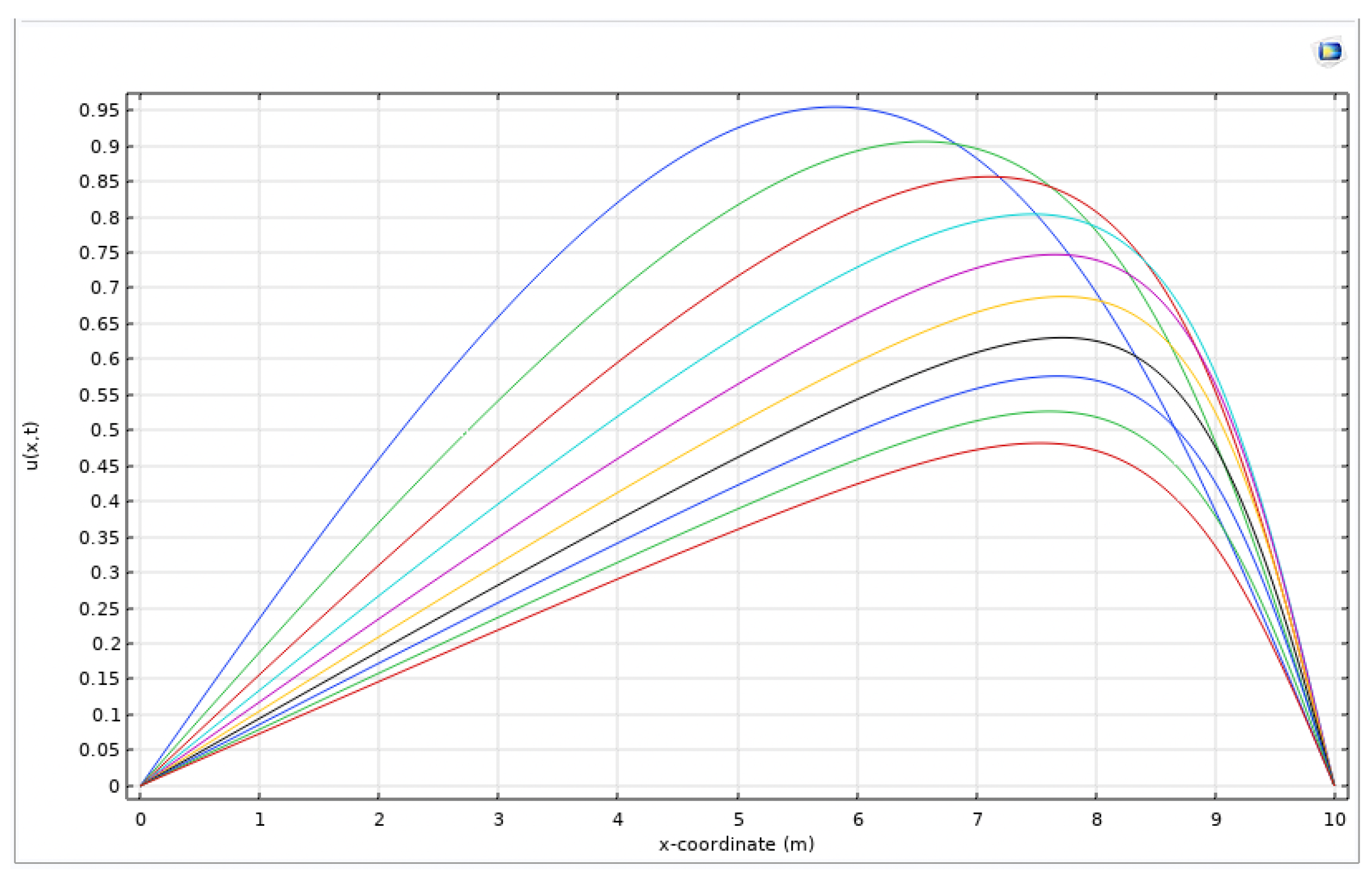
where $\nabla ={\partial }_x$ and $u=u(t,x)$. We construct the numerical solutions of problem (1) taking coefficients $e_a=0$, $d_a=1$, $a=0$, $f=0$, $\alpha =0$, $\gamma =0$, $\beta =u$ and $c=\nu \ast (-0.0264\ast abs(d(u,x))+0.5251)$ in the last equation. The Dirichlet boundary condition is applied on both ends of the computational domain.

Figure 1 shows the simulated solutions that were obtained for Burgers’ equation based on an Ellis law model with a small $\nu =1$. The velocity profile was shown for several instances of time. Since there is no stability and convergence analysis for the initial-boundary value problem, it was also challenging to experimentally find good combinations of the discrete time step size $\delta t$ and the spatial mesh size $\delta x$. For the particular set of data, convergence was obtained and a solution of the problem is obtained for $\delta t=0.01$ and $\delta x=0.01$.

It can be observed that within a finite time T, the solution u and its derivative ${\partial }_{x}u$ are bounded in $[0,10]$, as predicted by our theoretical results Theorem 1.

5. Conclusions

In this work, we first established the existence and uniqueness of weak solutions for the viscous Burgers’ equation based on the Ellis model, given by $\dot{\gamma }=\left[1+c{\left|\tau \right|}^{\alpha -1}\right]\tau$, for the isothermal flow of non-Newtonian fluids. Using the compact embedding theorem in Bochner spaces and key mathematical properties of the Ellis model, we proved the well-posedness of the initial boundary value problem in $L^2\left(0,T;W_0^{1,1+{\displaystyle \frac{1}{\alpha }}}(0,l)\right)$. Second, we developed a constructive algorithm to approximate solutions of the problem. A numerical experiment was conducted in COMSOL® Multiphysics to validate our theoretical findings, providing a computational illustration of the solution’s behavior. We note that there is no explicit expression for the inverse function on the right-hand side of (1); therefore, direct numerical implementation poses challenges when using Equation-Based Modeling in COMSOL. This difficulty was addressed by employing MATLAB to construct a polynomial approximation of $\tau ={\varphi }^{-1}\left(t\right)$, which allowed for a more convenient numerical formulation. These numerical results contribute to a deeper understanding of the mathematical framework for modeling shear-thinning and shear-thickening non-Newtonian fluids, demonstrating the applicability of mathematical analysis for the Ellis model in non-Newtonian fluid dynamics.

References

- Salih A.; Burgers’ Equation. Indian Institute of Space Science and Technology, Thiruvananthapuram, 2016.
- Bird R.B.; Armstrong R.C.; Hassager O. Dynamics of Polymeric Liquids, Volume 1: Fluid Mechanics; Wiley: New York, 1987.
- Hayat T.; Fetecau C.; Asghar S. Some simple flows of a Burgers’ fluid. Int J Eng Sci. 2006 44, 1423–1431. Acta Mech. 2006, 184, 1–13. [CrossRef]
- Tong D.; Shan L. Exact solutions for generalized Burgers’ fluid in an annular pipe. Meccanica. 2009, 44, 427–431. [CrossRef]
- Xue C.; Nie J. Exact solutions of Stokes first problem for heated generalized Burgers’ fluid in a porous half space. Non Linear Anal Real World Appl. 2008, 9, 1628–1637. [CrossRef]
- Vieru D.; Hayat T.; Fetecau C.; Fetecau C. On the first problem of Stokes’ for Burgers’ fluid, II: the Cases γ=λ2/4 and γ>λ2/4. Appl Math Comput. 2008, 197, 76–86. [CrossRef]
- Wei, D.; Borden, H. Traveling Wave Solutions of Burgers’ Equation for Power-law Non-Newtonian flows. Appl. Math. E-Notes 2011, 11, 133–138.
- Shu, Y.; Numerical Solutions of Generalized Burgers’ Equations for Some Incompressible Non-Newtonian Fluids. University of New Orleans Theses and Dissertations. 2015, 2051. https://scholarworks.uno.edu/td/2051.
- Zhapsarbayeva L., Wei D., Bagymkyzy B. Existence and Uniqueness of the viscous Burgers’ Equation with the p-Laplace Operator. Mathematics. 2025, 13(708), 1-14.
- Kheyfets, V.; Kieweg, S. Gravity-Driven Thin Film Flow of an Ellis Fluid. Journal of Non-Newtonian Fluid Mechanics.,2013, 202, 88–98. [CrossRef]
- Wadhwa, Y. D. Generalized Couette flow of an Ellis fluid. AIChE Journal, 1966, 12 (5), 890–893.
- Steller, R.; Iwko, J. Generalized flow of Ellis fluid in the screw channel: 2. Curved channel model. International Polymer Processing Journal of the Polymer Processing Society, 2001, 16, 249. [CrossRef]
- Abdulrahman A-B.; Mathieu S.; James N. H.; Roger I. N.;, Miguel M-G. Identification of Ellis rheological law from free surface velocity. Journal of Non-Newtonian Fluid Mechanics, 2019, 263, 15-23. ISSN 0377-0257. [CrossRef]
- Kumar, N.K. A Review on Burgers’ Equations and It’s Applications. Journal of Institute of Science and Technology. 2023, 28(2). [CrossRef]
- Alqahtani, A.; Khan, I. Time-Dependent MHD Flow of Non-Newtonian Generalized Burgers’ Fluid (GBF) Over a Suddenly Moved Plate With Generalized Darcy’s Law. Frontiers in Physics. 2020, 7, 214. [CrossRef]
- Brezis, H. Functional Analysis, Sobolev Spaces and Partial Differential Equations; Springer: Berlin/Heidelberg, Germany, 2011.
- Benia Y.; Sadallah B. Existence of solutions to Burgers equations in domains that can be transformed into rectangles. Electr. J. Differ. Equ. 2016, 157, 1-13.
- Dragomir S.S.; Adil Khan M; Abathun A. Refinement of the Jensen integral inequality. Open Math. 2016, 14, 221-228. [CrossRef]
- Aubin J-P. Un théorème de compacité. C. R. Acad. Sci. Paris. 1963, 256, 5042–5044.
- Evans L.C. Partial Differential Equations, 2nd ed.; American Mathematical Society: Providence, RI, 1998.
- Wade W.R. The Bounded Convergence Theorem. Am. Math. Mon. 1974, 81, 387–389. [CrossRef]
- Dwight H.B. Tables of integrals and other mathematical data. 3rd ed.; The Macmillan company: New York, 1957.
- Lindqvist P. Notes on the Stationary p-Laplace Equation, 1st ed.; SpringerBriefs in Mathematics: Switzerland, 2019.
Figure 1.
The solution for and a sequence of discrete times , plotted in different colors, as the velocity of the flow of the Ellis law fluid between two parallel plates at and .
Disclaimer/Publisher’s Note: The statements, opinions and data contained in all publications are solely those of the individual author(s) and contributor(s) and not of MDPI and/or the editor(s). MDPI and/or the editor(s) disclaim responsibility for any injury to people or property resulting from any ideas, methods, instructions or products referred to in the content. |
© 2025 by the authors. Licensee MDPI, Basel, Switzerland. This article is an open access article distributed under the terms and conditions of the Creative Commons Attribution (CC BY) license (http://creativecommons.org/licenses/by/4.0/).
Copyright: This open access article is published under a Creative Commons CC BY 4.0 license, which permit the free download, distribution, and reuse, provided that the author and preprint are cited in any reuse.