
Submitted:
05 February 2025
Posted:
06 February 2025
You are already at the latest version
Abstract
In this paper, we investigate the existence and uniqueness of solutions for the viscous Burgers’ equation for the isothermal flow of power-law non-Newtonian fluids $$\rho (\partial_t u + u \partial_x u)=\mu \partial_x \left(\left|\partial_x u \right|^{p-2} \partial_x u\right),$$ augmented with the initial condition $u(0, x)=u_0$, $0<x<L$ and the boundary condition $u(t, 0)=u(t, L)=0$, where $\rho$ is the density, $\mu$ the viscosity, $u$ the velocity of the fluid and $p$, $1<p<2$, $L, T>0$. Moreover, numerical solutions to the problem are constructed by applying the high-level modeling and simulation package COMSOL Multiphysics at small and large Reynold's numbers.
Keywords:
p-Laplacian
; Power-law Model
; Existence and Uniqueness
; Burgers' Equation
; Reynold's Number
; Sobolev Space
; COMSOL Multiphysics
1. Introduction
The Burgers’ equation, first introduced by J.M. Burgers, is a fundamental model for various physical processes, including shock wave propagation and turbulence [1]. Originally formulated for Newtonian fluids, the Burgers’ equation has been extensively analyzed; however, its generalization to non-Newtonian fluids—specifically those described by the power-law model—has received comparatively less attention for the case when [2]. We employ a particular case of the generalized Burgers’ equation formulated by Wei and Jordan [3], which was used to analyze acoustic propagation in power-law fluids. Traveling wave solutions of this equation were derived by Wei and Borden [4].
This paper’s main focus is to investigate the existence and uniqueness of weak solutions to the generalized viscous Burgers’ equation. The study is framed within the context of Sobolev spaces, which provide a robust mathematical environment for addressing weak solutions and ensuring appropriate regularity conditions [5].
Establishing the existence of weak solutions to nonlinear partial differential equations (PDEs) like the generalized Burgers’ equation has been well-studied in the context of Newtonian fluids [6,7]. However, extending these results to the power-law non-Newtonian fluids involves additional complexities due to the nonlinearity introduced by the fluid’s viscosity [8]. The unique solutions for the generalized Burgers’ equation based on power-law fluids remain largely unexplored for the case when , creating a gap in the current literature that this paper aims to address.
Wei and Jordan [3] established the following Burgers’ equation
as a model to study acoustic traveling waves in Power-law fluids with
, is the power-law index.
In this paper, we study the well-posedness and numerical solutions of a special case of the above equation with initial and boundary conditions
By using the dimensionless variables , , , to the last equation, we obtain the following problem, in which , , are still denoted by x, u, t
with and . In equation (1), stands for the Reynolds number, a dimensionless quantity determining the flow behavior based on the balance of inertial and viscous forces. The Reynolds number for power-law fluids is given by
where L and represent the characteristic length and velocity, respectively (see, for example, [9]). The Reynolds number significantly influences the stability of the flow and the type of flow regime observed. Our numerical simulations demonstrate this. When in case , equation (1) becomes a well-known Burgers’ equation for a Newtonian fluid
The well-posedness of the viscous Burgers’ equation for Newtonian fluid has been studied intensively in the literature (see, for example, [6,10,11]). To our knowledge, the well-posedness of the problem (1) has not been studied before. In our work, we prove the result concerning the existence, uniqueness, and regularity of a solution to the Burgers equation with p-Laplasian right-hand side (1).
Multiplying the equation of (1) by a test function , and integrating by parts from 0 to 1, we convert the initial boundary value problem (1) to the following integral equation
for all , and .
Definition 1.1.
Now, we present the main result of the work.
Theorem 1.2.
Let . Then there exists a unique solution of (1) such that , in the sense of Definition 1.1.
In Section 2, we state some preliminary information needed to study the well-posedness of the problem (1), formulated in the weak form (2). Section 3 consists of two subSection 3.1 and Section 3.2. We obtain the existence result in Section 3.1 and establish the uniqueness of the solution in Section 3.2. Moreover, in Section 4, we construct the numerical solutions for the various values of the Reynolds number , by using the COMSOL PDE solver with some numerical manipulations to avoid singularity in at points where .
2. Preliminary
We present well-known facts that we will use to prove Theorem 1.2. The Gronwall’s inequality, some Sobolev inequalities, and the monotonicity of the p-Laplacian operator defined by are required to establish the main result.
Recall that and are the standard spaces of Lebesgue and Sobolev, respectively, for and . For any Banach space X, we define to be the space of measurable functions such that
for and if . is a Banach space [12].
Proposition 2.1
(The differential form of Gronwall’s inequality [13]).
- (i)
-
Let be a nonnegative, absolutely continuous function on , which satisfies for a.e. t the differential inequalitywhere and are nonnegative, summable functions on . Thenfor all .
- (ii)
-
In particular, ifthen
Proposition 2.2 (Poincaré’s inequality
for each , the constant C depending only on and U.
In particular, for all ,
Next, we recall the Bounded Convergence Theorem.
Proposition 2.3
([14]). If f is a Lebesgue measurable function defined on a closed, bounded interval [a,b], with its norm for defined by
and norm
If is a sequence of measurable functions and M is a positive constant such that
and a.e. then
for any p satisfying .
Now, we state the well-known Theorem.
Proposition 2.4
([15]). The space is complete and separable if .
Proposition 2.5 (Jensen’s inequality)
[16] Let be a measure space with and let be a convex function defined on an open interval I in if is such that , then
Proposition 2.6
([17]). If a sequence of continuous functions converges uniformly on to , then f is continuous on A.
3. Existence and Uniqueness
3.1. Existence
In this subsection, we will prove the existence of solutions to the integral equation (2).
Firstly, we choose the basis defined as a subset of the eigenfunction of the Laplacian for the Dirichlet problem.
where
for .
Since is an orthonormal basis in , then is also an orthonormal basis in . Then for we can write
with and the series is converges in .
Hence, the approximate solution can be represented as follows
Moreover, we suppose that satisfy the following approximating problem
for all , .
Remark 3.1.
The coefficients can be chosen such that in .
Furthermore, we prove the lemma concerning the solution of approximate problem (8).
Lemma 3.2.
There exists a positive constant independent on n, that satisfies the following inequality
for all .
Proof.
Taking and substituting into equation (8), we obtain
The first term of (9) can be written as follows
Lemma 3.3.
There exists at least one solution of the approximating problem (8) such that .
Proof.
It is obvious that
We note that
Now, we represent the approximate equation (8) in the following form
for .
The substitution (14) into (15) gives
for . We find the derivative of (6) with respect to t, then by (13), the integral on the left-hand side of (16) can be written as below
First integral on the right-hand side of (16), we rewrite as follows
for . Here is bounded on , since
with constant numbers (see (5)).
Equation in (4) implies that
By equation (20), we transform the second integral on the right-hand side of (16) in the following way
for .
Thus, substitutions (17), (18), and (21) into (16) lead us to the following homogeneous ordinary system of equations with respect to t
for .
Furthermore, we introduce the following notations
with from (19).
Therefore, by using our notations, the homogeneous system of ODE (22) can be written as follows
Here is the Hadamard product of two vectors specified by the following formula
The first term on the right-hand side of (24) is the linear. The second term on the right-hand side of (24) is a homogeneous system of ODE.
Now we denote the second term of (24) by .
So, equation (23) can be rewritten as the homogeneous system of equations
We show that
is bounded and continuous.
If , then
Notice that
is bounded and continuous in .
We only consider to prove that
is bounded and continuous at one point where . So, each integrand of the following integrals
is bounded, if . By Lemma 3.2, we have
Equation (12) implies that . Hence, is bounded in . Then there exists sequence that converges to in for . Moreover, this sequence satisfies the estimates
Consequently, there exist functions , such that and . Functions , are continuous and uniformly converge to , in for all . Then by the Proposition 2.6 on continuity of the sum of uniformly convergent series, functions , in are also continuous in for all . Thus, and .
Therefore, a system of equations (26) satisfies the condition of the existence of the homogeneous system of ODE. The right-hand side of equations (26) is continuous for all on the bounded domain . Consequently, there exists a unique solution
of equation (26) on that satisfies the initial condition or for .
The proof of the lemma is complete. □
We are now ready to prove the following lemma.
Lemma 3.4.
There exists a weak solution of the equation (2) such that .
Proof.
Thus, by Lemma 3.3 there exists a weak solution of the approximating problem (8) in . Moreover, by Lemma 3.2 the sequence of functions and are bounded in . Therefore, by Proposition 2.4, the sequence has a subsequence that converges to some . We denote this subsequence still by , we obtain
which implies
for a.e. t.
Since is complete space, then any has a limit such that . Since , hence . Therefore . □
4. Uniqueness
In the following lemma, we establish some auxiliary statements that we apply in the proof of Lemma 3.6.
Lemma 3.5.
Let . Then there exists the positive number such that .
Proof.
Since , then the Embedding theorem
implies that is continuous on . Hence, by the Extreme Value theorem, if a function is continuous on a closed interval, it attains its maximum and minimum values on this interval. Consequently, there exists the positive number such that . □
Now we prove the uniqueness result.
Lemma 3.6.
If , the integral equation (2) has a unique weak solution.
Proof.
Assume that there exist two solutions of equation (2), and . Taking in the equation (2) and denoting by , we obtain
with .
We note that
Therefore,
Hence, the second integral of (30) can be represented in the following way
By invoking Lemma 3.5, we bound the third integral on the right-hand side of (32)
where .
Integrating by parts the second term on the right-hand side of equation (32), we have the same estimate as (33),
So, we have the following estimate
for the second integral of (30).
Furthermore, we bound the third term on the left-hand side of (30). Therefore, we apply the following inequality [18]
for , and , to the last term of the equation (30)
The left-hand side of (35) can be written as follows
By Jensen’s inequality, we bound the norm in the last equation from below
The last inequality and the inequality (35) implies that
Using Poincare’s inequality (2.2) to the last inequality leads us
Combining the similar terms in the last inequality, we conclude that there exists a non-negative constant K such that
with .
4. Numerical Part
In this section, we first create a data set by solving numerically the Reynolds number with prescribed Power-law rheology parameters. The corresponding parameters and values for the Reynolds number are listed in Table 1. Problem (1) is solved using the finite element software COMSOL Multiphysics 6.0. To apply the software COMSOL, the equation in (1) has been written in a standard form for the solver
where and . We construct the numerical solutions of problem (1) taking coefficients , , , , , , and in the last equation. The Dirichlet boundary condition is applied on both ends of the computational domain.
Figure 1 shows the simulated solutions obtained for the Burgers’ Equation based on a Power-law model with three different Reynolds numbers. In each case, the velocity profile has been shown for several instances of time. It can be observed that within a finite time T, the solution u and its derivative are bounded in , as predicted by our theoretical results.
5. Conclusions
This work proves the existence and uniqueness of weak solutions of the viscous Burgers equation for the isothermal flow of power-law non-Newtonian fluids with initial and boundary conditions. A numerical experiment on COMSOL Multiphysics was conducted, confirming the theoretical part.
Acknowledgments
The first and third authors are supported by the Ministry of Science and Higher Education of the Republic of Kazakhstan Grant No. AP23489433.
References
- Burgers, J.M. A Mathematical Model Illustrating the Theory of Turbulence. Adv. Appl. Mech.. 1948, 1, 171–199. [Google Scholar]
- Bird, R.B.; Armstrong, R.C.; Hassager, O. Dynamics of Polymeric Liquids, Volume 1: Fluid Mechanics; Wiley: New York, 1987. [Google Scholar]
- Wei, D.; Jordan, P.M. A note on acoustic propagation in power-law fluids: Compact kinks, mild discontinuities, and a connection to finite-scale theory. Int. J. Nonlin. Mech. 2013, 48, 72–77. [Google Scholar] [CrossRef]
- Wei, D.; Borden, H. Traveling Wave Solutions of Burgers’ Equation for Power-law Non-Newtonian flows. Appl. Math. E-Notes. 2011, 11, 133–138. [Google Scholar]
- Adams, R.A.; Fournier, J.J.F. Sobolev Spaces, 2nd ed.; Academic Press: The Netherlands, 2003. [Google Scholar]
- Hopf, E. The partial differential equation ut+uux=μuxx. Commun. Pure Appl. Math. 1950, 3, 201–230. [Google Scholar] [CrossRef]
- Kruzhkov, S.N. First Order Quasilinear Equations in Several Variables. Math. USSR-Sb 1970, 10, 217–243. [Google Scholar] [CrossRef]
- Lions, J.L. Quelques Méthodes de Résolution des Problèmes aux Limites Non Linéaires; Dunod: Paris, 1969. [Google Scholar]
- Wei, D. Existence and uniqueness of solutions to the stationary power-law Navier-Stokes problem in bounded convex domains. Proceedings of Dyn. Syst. Appl. 2001, 3, 611–618. [Google Scholar]
- Cole, J.D. On a quasi-linear parabolic equation occurring in aerodynamics. Q. Appl. Math. 1951, 9, 225–236. [Google Scholar] [CrossRef]
- Temam, R. Navier-Stokes Equations: Theory and Numerical Analysis; Elsevier Science Publishers B.V.: Amsterdam, 1984. [Google Scholar]
- Benia, Y.; Sadallah, B. Existence of solutions to Burgers equations in domains that can be transformed into rectangles. Electr. J. Differ. Equ. 2016, 157, 1–13. [Google Scholar]
- Evans, L.C. Partial Differential Equations, 2nd ed.; American Mathematical Society: Providence, RI, 1998. [Google Scholar]
- Wade, W.R. The Bounded Convergence Theorem. Am. Math. Mon. 1974, 81, 387–389. [Google Scholar] [CrossRef]
- Lions, P.L. The concentration-compactness principle in the calculus of variations. The locally compact case, part 1. Ann. Inst. Henri Poincare (C) Anal. Non Lineaire 1984, 1, 109–145. [Google Scholar] [CrossRef]
- Dragomir, S.S.; Adil Khan M; Abathun A. Refinement of the Jensen integral inequality. Open Math. 2016, 14, 221–228. [Google Scholar] [CrossRef]
- Hunter, J.K. An Introduction to Real Analysis. https://www.collegesidekick.com/study-docs/3018040 (accessed 2014).
- Lindqvist, P. Notes on the Stationary p-Laplace Equation, 1st ed.; SpringerBriefs in Mathematics: Switzerland, 2019. [Google Scholar]
Figure 1.
Velocity components for the flow of Power-law fluid.
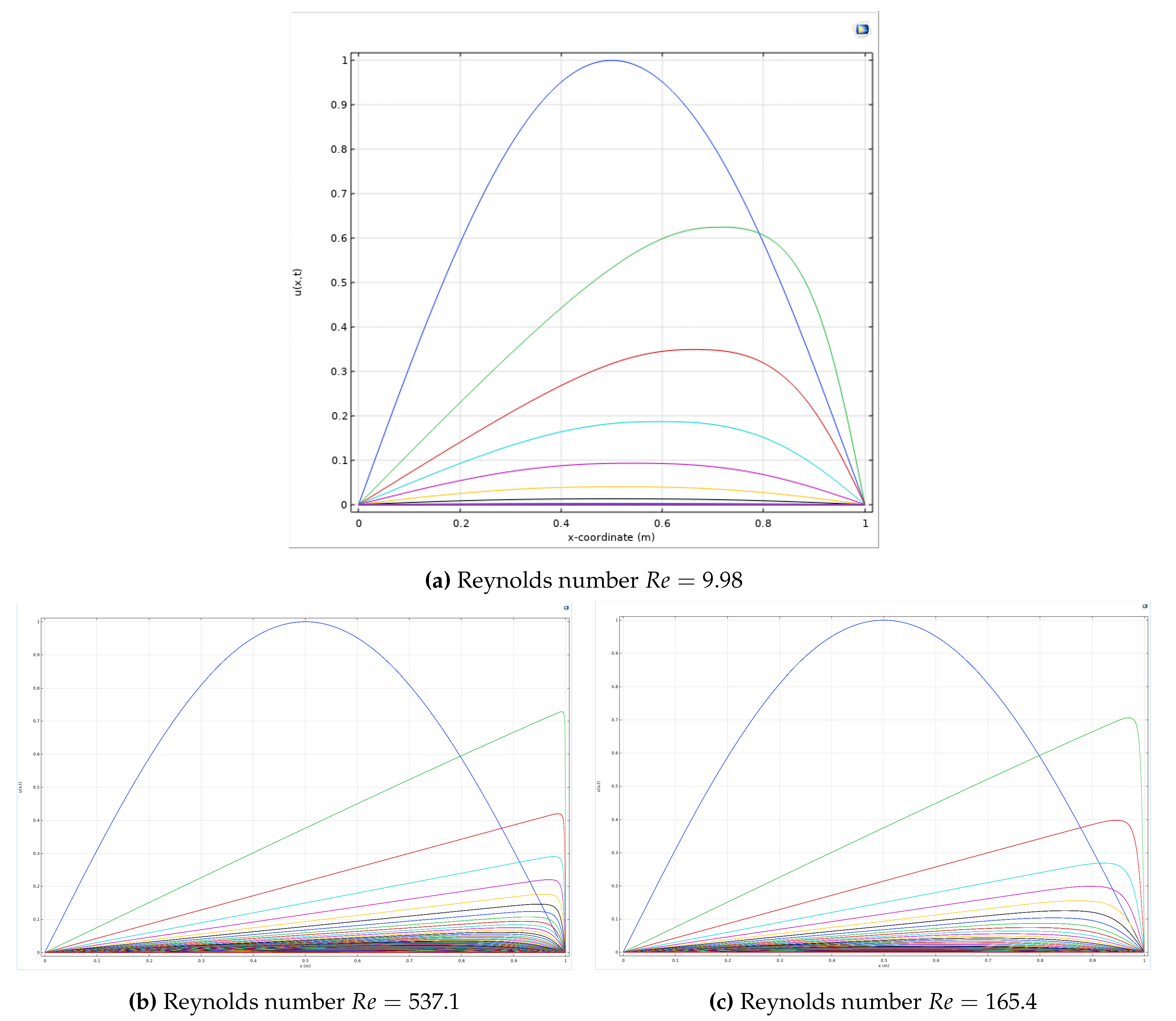

Table 1.
Parameter values for Power-law fluids.
| Parameters | Case 1 | Case 2 | Case 3 |
|---|---|---|---|
| 1000 | 1100 | 1200 | |
| u | 0.10 | 10.0 | 2.00 |
| L | 0.05 | 0.05 | 0.10 |
| n | 0.70 | 0.70 | 0.80 |
| K | 1.00 | 2.00 | 2.00 |
| 1000 | 200 | 500 | |
| 9.98 | 537.1 | 165.4 |
Disclaimer/Publisher’s Note: The statements, opinions and data contained in all publications are solely those of the individual author(s) and contributor(s) and not of MDPI and/or the editor(s). MDPI and/or the editor(s) disclaim responsibility for any injury to people or property resulting from any ideas, methods, instructions or products referred to in the content. |
© 2025 by the authors. Licensee MDPI, Basel, Switzerland. This article is an open access article distributed under the terms and conditions of the Creative Commons Attribution (CC BY) license (http://creativecommons.org/licenses/by/4.0/).
Copyright: This open access article is published under a Creative Commons CC BY 4.0 license, which permit the free download, distribution, and reuse, provided that the author and preprint are cited in any reuse.


