Submitted:
20 May 2025
Posted:
20 May 2025
You are already at the latest version
Abstract
Snow water equivalent (SWE), an essential parameter of snow, is largely studied to understand the impact of climate regime effects on snowmelt patterns. This study developed a Siamese Attention UNet (Si-Att-UNet) model to detect daily change events in the winter season. The daily SWE change event detection task is treated as an image content comparison problem in which the Si-Att-UNet compares a pair of SWE maps sampled at two temporal windows. The model detected SWE similarity and dissimilarity with an F1 score of 99.3% at a 50% confidence threshold. The change events were derived from the model’s prediction of SWE similarity using the 50% threshold. Daily SWE change events increased between 1979 and 2018. However, the SWE change events were significant in March and April, with a positive Mann-Kendall test statistic (tau = 0.25 and 0.38, respectively). The highest frequency of zero-change events occurred in February. A comparison of the SWE change events and mean change segments with those of the Northern Hemisphere’s climate anomalies revealed that low temperature and low precipitation anomaly reduced the frequency of SWE change events. The findings highlight the influence of climate variables on daily changes in snow-related water storage in March and April.
Keywords:
Siamese attention network
; snow water equivalent
; daily snow variability
; structural similarity
; snow‐related change events
; climate change
1. Introduction
Snow is an essential landcover type in the cold regions and plays a critical role in the Earth’s hydrology, surface energy balance, and climate regime variability. It is estimated that approximately 65% of the Canadian landmass is covered with snow during the winter [1]. Snowmelt produces water that feeds freshwater ecosystems and contributes to irrigation [2]. Snow cover, in combination with ice melt deposition in the ocean, further influences the sea energy budget and ice mass balance, as well as aquatic species' productivity[3]. Snowfall also modulates sea ice thermodynamics by forming thicker snowpacks that reduce heat loss[4].
Snow stratigraphy and physical characteristics respond naturally to environmental variables. However, climate warming is likely to exacerbate changes in snow parameters with unpredictable impacts on humans and ecosystems. Rapid daily change in the snowmelt process, primarily driven by human-induced climate warming, could trigger catastrophic events such as floods, landslides, and hydropower system collapse [5]. For example, snowmelt-driven avalanches impact the safety of humans and infrastructure[6], [7]. Additionally, earlier snowmelt off alters the timing and volume of snow-related runoff, increasing the occurrence of spring flooding and summer droughts [8,9,10]. Soil temperature, water availability, and soil microbial respiration are also affected by snow dynamics [11,12,13]. Furthermore, early snowmelt has deleterious consequences on leisure activities such as over-snow vehicle recreation and skating [14,15].
Snow water equivalent (SWE) – the amount of water that will be yielded if a given snowpack melts, snow cover extent (SCE) – the area of ground covered by snow, and snow depth (SD) – the vertical depth of ground snow, are highly sensitive snow parameters and thus sentinels of climate change. These snow parameters have been extensively used to investigate the effects of climate change and global warming in the Arctic and other cold regions. Significant progress has been made toward characterizing trends in SWE, snow depth, and snow density [16], evaluating SCE and snow properties [17]. For instance, analysis of gridded snow data has shown declining SWE trends in Eastern and Western Canada in March [18]. Using interpolated data, it was also found that SD is decreased in Finland [20]. Similarly, Pulliainen et al. [16] used GlobSnow’s v3.0 dataset to illustrate that snow mass is declining across North America in March. In a related study, SCE has been shown to decline in the Northern Hemisphere [19]. However, as the ensemble of available SWE data is derived from varying inputs, an accurate understanding of snow variability, climatology, and historical trends would require comparing the ensemble of available data products [20].
Despite the progress in snow trend studies, snow is not a consistent sentinel of climate-forcing; snow is influenced by diverse variables, including the snow-albedo feedback [21,22,23]. Furthermore, the relationship between seasonal snow and climate variables is uncertain and non-linear [24]. For example, snow cover response to temperature and precipitation varies with latitude, whereas excessive precipitation biases the estimates of snow distribution [25,26]. In many studies, snow trend analysis is based on selecting reference periods and averaging time series snow observations [27]. Also, snow data in March is frequently used to analyze SWE trends[28]. Comparative analysis of snow trends during all the winter months will provide valuable information on snow parameter response to climate variables.
Quantifying changes in snow parameters at high temporal resolution is an effective method for inferring the effects of global climate trends on snow dynamics during the winter season [29]. Spatial-temporal pattern of daily SWE melt, however, is largely understudied, partly due to low signal-to-noise ratio in daily SWE, uncertainty in gridded SWE data products, and the tendency for algorithms to detect internal variability in SWE that is not directly related to the underlying climate variables [25,30]. Furthermore, given that detecting and attributing changes in snow is not a straightforward task [26], methods invariant to stochastic internal variability and seasonal patterns of snow spatial structure are crucial for obtaining accurate estimates of changes in snow parameters.
Computer vision and deep learning methods have excelled at pattern recognition involving the comparison of spatial and temporal variability in Earth Observation data [31]. The U-Net, a fully convolutional CNN, is one such deep learning model [32]. To overcome the limitations of the classical U-Net, sophisticated variants such as the residual U-Net, Dense U-Net, and the Attention U-Net were developed [15,33,34]. Multiscale attention transformers have been introduced to detect change [36,37,38]. The fully convolutional feature extraction, skip or residual connections, and an Encoder-Decoder module in the U-Net ensure the models retain spatial information that characterizes local image structures.
This study builds on Malik and Robertson's [31] previous work on change detection in SWE using the U-Net model. In the wake of climate change, monitoring snow processes at daily temporal resolution is becoming more imperative to improving human well-being and economic viability, as well as predicting, managing critical infrastructure, and adapting to snow-related disasters. Therefore, the overarching objectives of this study are to: (a) demonstrate Siamese Attention UNet’s capability to detect daily similarity and variability in SWE, (b) estimate the frequency of daily SWE change events during winter, and (c) link SWE change events to climate anomalies.
2. Progress in Snow Trend Analysis
Snow data collection began with in situ weather stations, which remain operational to date. The Snow Telemetry (SNOTEL) and Canada’s SWE (CanSWE) are typical point-wise in situ snow data derived using a constellation of stations across the conterminous United States and Canada, respectively [39]. These datasets have proved vital for snow parameter studies [18]. Point-wise snow measurements, however, tend to lack complete spatial continuity. To address this inherent discontinuity, gridded snow data products have been developed using in situ data combined with spatial interpolation, machine learning, passive microwave, and real-analysis techniques [40,41,42].
Gridded snow data products are derived using three main methods: remotely sensing, spatial interpolation, and reanalysis. These datasets encompass the major snow parameters - SWE, SD, and SCE. Like all gridded data, the utility of the snow data products is dictated by both their temporal and spatial dimensions, as well as the magnitude of bias in the estimates of snow parameter distribution. While local-scale analysis requires high to medium spatial resolution, regional and continental-scale analysis can be conducted using coarse-resolution data products. At this current juncture, coarse spatial resolution SWE (e.g., 4 km – 25 km) time-series data products are prevalent, partly due to the challenges inherent in passive microwave, interpolation, and reanalysis techniques.
Snow depth is a crucial parameter for studying snow dynamics. Statistical interpolation methods have been employed to derive gridded SD for Finland and North America [43,40]. More recently, machine learning-driven methods were applied to fuse snow depth and the original gridded snow depth products, producing an improved SD data [42]. SD data is one of the primary inputs that snow models assimilate to generate gridded SWE [40]. Despite their relevance as inputs to snow models, SD generated through passive microwave techniques incur bias and underestimate SD, especially at over 100 cm depth [20]. For example, changes in passive microwave input and snow density parameters affect the quality of SWE data [44].
The Global Snow Monitoring for Climate Research’s (GlobSnow) SWE dataset is a typical example in which microwave remote sensing and synoptic weather station climate data are fused to derive SWE over a hemispherical scale [41,45]. GlobSnow SWE data incurs spatial discontinuity in mountainous regions. Consequently, research into developing snow data products for mountainous regions is an active area of scientific endeavour. Further, GlobSnow’s v 3.0 resolution of 25 km × 25 km limits analysis at sub-kilometer scales. The European Space Agency’s Snow Climate Change Initiative (Snow_cci) data mitigates this challenge partially by improving SWE spatial resolution to approximately 11 km × 11 km [46].
Reanalysis, based on models for snow retrieval by assimilating ground weather stations data, is another type of gridded snow data product. Reanalysis data, however, tend to possess coarse spatial resolution and may come with profound bias as well as uncertainty in SWE variability [47]. Given the plethora of snow data products and their inherent variability in snow parameter representation, robust algorithms and a combined analysis of the available datasets will likely yield informed insights into snow response to climate change and global warming.
3. Materials and Methods
Figure 1 depicts our study location in the cold regions of Canada. The provinces – Alberta, Yukon, and Northwest Territories cover a pronounced proportion of the study area. As can be observed from Figure 1, snow persists in the cold regions for longer days, beyond April, than in other areas of the Canadian land mass. We used the GlobSnow’s v3.0 SWE data, derived from the estimates of SWE using satellite-based passive microwave technology - Scanning Multichannel Microwave Radiometer, and Special Sensor Microwave/Imager (SSM/I) and Special Sensor Microwave Imager/Sounder (SSMIS) instruments. GlobSnow v3.0 incorporates bias-correction procedures that are implemented to account for uncertainties in the estimation of SWE. Additional details on this version of SWE data are provided in [37].
3.1. Training Sample Processing and Labeling
The SWE maps were dichotomized into “Change” (Negative Pairs) and “No Change” (Positive Pairs) instances. Given the inherent spatial variability observed in the SWE maps, we deployed a computer vision metric – the Structural Similarity (SSIM) index to objectively label the training sample. The SWE data that differed by one day were labeled as positive pairs (No Change), whereas the SWE maps that were two or more days apart were labeled as negative pairs (Change). We used SWE data from 1979 to 2001 for model development, and data from 2002 to 2018 for independent validation of the model’s performance. The pink bounding box in Figure 1 depicts the input data, consisting of 72 × 72 pixels. Further details and guidelines on the deployment of the SSIM index for data labeling are outlined in Malik and Robertson [31].
3.2. Siamese Attention U-Net Architecture
Our Si-Att-UNet with the attention module is depicted in Figure 2. While the Siamese network allows the model to learn shared feature representations from two input images, the U-Net with encoder-decoder architecture and skip connections simultaneously stimulates the learning of significant features for SWE representation and reconstruction. The Attention module is a form of “spatial excitation” which can potentially result in the extraction of significant features. Thus, the Siamese Attention U-Net holds the potential to learn spatial structure encoding SWE variability and the underlying spatial processes (e.g., fraction of precipitation falling as snow and sub-zero temperatures) that generate SWE. Given that GlobSnow’s data spatial resolution is 25 km × 25 km, a careful selection of the model’s filter parameter is essential. Relating filter parameters to the field of view (FoV) of the neurons in the model’s first layer, the contextual window size equates to FoVs of 50 km × 50 km and 75 km × 75 km for the 2 × 2 and 3 × 3 filters, respectively. The spatial scale associated with the FoV increases in the higher layers of the network, resulting in the extraction of coarse resolution features. For daily change detection, a smaller filter parameter will likely capture the underlying local structure in SWE variability. Consequently, a 2 × 2 filter was adopted to effectively detect localized changes in SWE distribution.
3.3. The SSIM Index and the Contrastive Loss Function
The expression for the SSIM index, proposed by Wang et al. [48] is given below.
are represent the mean of a block of pixels in image x and y, respectively; , are respectively the variances of x and y while are x and y covariances; are stabilizing constants. Wang et al. [48] provide extensive mathematical details on the SSIM index
The learning paradigm under the contrastive loss ensures that similar data pairs receive high scores while dissimilar data pairs receive lower scores. Consequently, the SSIM index value is maximized for positive (No Change) and minimized for negative (Change). The contrastive loss function, defined to operate with the SSIM index, is written as follows:
Where denotes contrastive loss, and are margin and SSIM index, respectively; denote a pair of SWE images, and represents labels. We emphasize that for positive pairs (No Change SWE), (i.e., ) and for negative pairs (Change SWE), (i.e., ). Additionally, we note that the SSIM’s upper bound is 1, which aligns with the margin parameter often adopted for the contrastive loss function. An extended mathematical illustration of how the SSIM index fits into the objective function’s optimization process is found in Malik and Robertson [31].
3.4. Deriving the Frequency of Daily Snow Water Equivalent Change Events
To estimate daily SWE change events, we first compute daily similarity vector – as illustrated below:
where and represent day and month, respectively; denotes a SWE map observed on the ith day. The model term represents our Si-Att-UNet. We applied a 50% threshold to the resulting values to derive the frequency of change events for each month. We adopted this threshold by examining the distribution of the model’s predictions of on the independent validation data. At values greater than or equal to 50%, the SWE map pairs were closely identical and could not be easily dichotomized by the human visual system. Thus, this threshold represents the “No Change” scenario, whereas values below this threshold were treated as change events.
3.5. SWE Change Point Detection
We utilized the changepoint package in R to compute change segments in each month. The package implementation follows the Prune Exact Linear Time (PELT) and Segment Neighborhood Identification (SegNeigh) algorithms[49,50]. There are several adjustable parameters associated with PELT and SegNeigh, the choice of which influences their sensitivity to change point detection and the length (i.e., temporal dimension) of segments detected. The PELT and SegNeigh methods were extensively explored with varying penalty terms for consistency and stability of change segments. We found that the SegNeigh generated change points with reasonable temporal dimensions. The PELT method consistently generated segments as short as one or two timestamps, regardless of the penalty magnitude. The manual penalty parameter was adopted, and the values were set to 0.5, and 0.8 for mean and variance change segment computation, respectively.
4. Result
4.1. Model’s Accuracy Metrics
The model’s accuracy on the prediction of SWE similarity and change was evaluated using the metrics - true positive rate (TPR), true negative rate (TNR), false positive rate (FPR), false negative rate (FNR), Precision (PR), F1 score, and overall accuracy (OA) to assess the models’ prediction of SWE similarity and change. The models’ accuracy from thresholds 40% – 50% is presented in Table 1 below.
4.2. Daily Snow Water Equivalent Change Events
Figure 3 presents daily count of SWE change events from January to April. Linear regression, Mann-Kendall (KM) trend test (Table 2), and change point analysis were performed to detect trends in the daily SWE change events. The statistics, S, tau, and p-value are derived from MK test, while the R2 is estimated from linear regression. It can be observed that in January and February, there were no statistically significant trends in the frequency of change events. Conversely, a significant increase in the number of change events occurred in March and April. However, SWE change events exhibited a profound increase in April (tau = 0.38, p-value < 0.05) than those observed in March. Moreover, the change events were more frequent in April than in January, February, and March. Between 1979 and 1987, the change events were relatively low. The frequency of change events further declined substantially between 1988 and 1993. Contrarily, the change events consistently increased after 1994. April recorded the highest amount of non-zero change events (one zero change in 1994). The maximum number of change events (i.e., 20 – 21) occurred in April between 2005 and 2007. January, February, and March recorded non-zero change events for two to three consecutive years.
4.3. Daily SWE Change Segments
Figure 4 presents the mean change segments for the change events in the four months. Each segment’s length is the width of the horizontal lines, while the vertically oriented lines demarcate the end of one segment and the beginning of another. The change point algorithm consistently detected change segments from 1979 to 1987 in all the months. However, March depicts a longer change segment spanning 1979 to 1999. Again, a relatively longer segment (2009 to 2018) was detected in March and April, yet the mean change point was higher in April (~12 days) than in March (~ 9 days). It is also interesting to note that a major segment was detected in January, February, and April, stretching from 1989 to 2004. Conversely, this segment appeared fragmented into two minor change points in March.
4.4. Temperature Anomaly
Figure 5 presents NOAA’s Land and Ocean surface temperature anomalies over the Northern Hemisphere from 1979 to 2018. The red line denotes change segments detected by the change-point algorithm, whereas the circles are monthly temperature anomalies. For February, the temperature anomaly remained low from 1979 to 1994. This temporal window was detected as a mean change segment. Temperature anomalies remained relatively low in the earlier decades (i.e., 1979 – 1999) for the rest of the months. Conversely, the anomalies increased dramatically in the subsequent decades. This rise in anomaly was detected as the second change point in the temperature anomaly time-series. The highest anomaly readings were observed after 2015 for all the months. Sub-zero temperature anomalies occurred in all the months except March. Overall, there were two consistent major change segments for all the months; one occurring in the earlier decades (1979 – 1999), and another in the latter decades (2000 – 2018).
4.5. Precipitation Anomaly
Figure 6 depicts the mean change points derived from NOAA’s Land and Ocean precipitation anomaly data. There were three major change segments in January and February, and four in March and April. The change points and segments for January and February exhibited a consistent pattern for the first 1.5 decades (1979 – 1994) as well as the last decade (2009 – 2018). However, it is worth emphasizing that the mean of the change segments was higher in January (i.e., 70 mm) than in February (i.e., 58 mm). March and April also elicited similarities in the pattern of mean change segments. For example, the lengths of the first change segment between 1979 and 1984 were approximately congruent. The mean of the segments varies marginally, reaching a maximum of 66 mm and 68 mm for March and April, respectively. The last mean change segments in March and April span a similar temporal window (i.e., 2000 – 2018) with nearly identical mean values (~ 63 mm). A major change segment was observed in March between 1985 and 1999. In a similar vein, between 1985 and 1990, a major change segment (mean of ~ 62 mm) was detected in April. Additionally, a change segment occurred between 1990 and 1999. It is worth noting that the last decade (2008 – 2018), incurred major change segments for all the months.
5. Discussion
The daily SWE change events detection task was cast as a computer vision problem in which a pre-trained Si-Att-UNet model was deployed to compare a pair of SWE maps sampled at two temporal windows – the current time and future time. The values were flagged as “Change” or “No change” instances if a threshold value was exceeded. Change events were detected using a threshold of 50% daily SWE change events. As shown in Table 1, except for TPR, which remained 100%, all the other accuracy metrics varied as the threshold parameter was altered from 40% to 48%. There was a trade-off between FNR and FPR, whereby increasing the threshold beyond 50% resulted in an elevated FPR or reduced TPR while increasing TNR. This behaviour of the model implies that No Change instances of SWE are easy to detect, even at very low threshold parameters. The opposite is true for the Change instances; thus, a higher threshold parameter was required to detect dissimilar SWE. This highlights the challenging nature of change detection problems. Although the number of FPR began to increase as the threshold increased, the 50% threshold appeared to be the optimum value for maximizing the model’s accuracy (F1-score).
Mann-Kendall trend test and linear regression were performed on the threshold values to estimate the significance in the direction and magnitude of daily change events as in [14,51]. Daily SWE change events trends in April (tau = 0.38) and March (tau = 0.25) exhibited a statistically significant increase from 1979 to 2018. January and February showed no significant trend in the frequency of change events. The relatively high frequency of change events in April is indicative of pronounced daily variability in snow distribution and melt-off patterns. This characteristic daily melt-off is obvious in the April 2018 SWE maps depicted in Figure 1. As can be observed from the figure, the SWE melt-off pattern is more pronounced from April 24 to 29. The tau value of 0.38 (Table 2) supports an increasing snow melt-off pattern in April. The daily melt-off is predominantly a function of changes in temperature and precipitation[17,52]. Given that the frequency of change events was high in April and increased over time, it can be postulated that climate-forcing agents significantly altered the snow regime in April. However, we emphasize that a daily localized comparison of temperature and precipitation over the study area is required to substantiate this conclusion. The SegNeigh change-point algorithm revealed consistent change segments in the earlier period (i.e., 1979 – 1987) across all months and years. Shorter segments are indicative of the varying influence of the effects of the climate drivers (i.e., temperature and precipitation)[53,54,55]. The mean of the segments tended to occur at higher change event frequencies in January, February, and April; this suggests a high variability in daily snow deposition processes (e.g., low temperature and high fraction of precipitation falling as snow), particularly in January and February.
The pattern observed in April SWE distribution is related to a consistent decline in snow parameters over the years. The last decade of April (i.e., 2008 – 2018) exhibited the highest frequency of change events. This period recorded the longest mean change segment among all the months. Daily SWE melting process evolves more rapidly in April, resulting in low SWEsim values, and thus increasing the frequency of daily change events. Contrarily, the mean change segments for March were associated with lower change event counts, especially in the first two decades (i.e.,1979 – 1999). Snow parameters (e.g., snow depth, snow density, and snow cover extent) tend to reach their peak in March [28]; this implies the snow parameters were highly stable in March, resulting in higher values and consequently, a low frequency of change events.
The NOAA’s Land and Ocean Surface temperature and precipitation anomaly at a monthly temporal resolution over the Northern Hemisphere holds the potential to elucidate the effects of climate-forcing variables on the snow regime and related cryosphere processes. Figure 5 and Figure 6 present average monthly temperature and precipitation mean change points over 40 years. The temperature anomaly trends depicted an inverse relationship with interannual SWE change events. As quantitatively derived from the NOAA data, the temperature anomalies increased by +0.25oC/decade (January), +0.26oC/decade (February), and +0.28oC/decade (March and April)[56]. Temperature anomalies were lower in the earlier decades (i.e., 1979 – 1987); this coincides with the fewer change events detected in this temporal window. The latter years (1990 – 2018) were characterized by high temperature anomalies; again, this concurs with the high frequency of daily change events observed after 1990.
The trends in average monthly precipitation show variable patterns over the Northern Hemisphere. Precipitation anomalies increased marginally in January (+0.01 mm/decade) and February (+0.02 mm/decade). March and April recorded a significant reduction in precipitation anomalies, corresponding to -0.32 mm per decade and -0.3 mm/decade, respectively[56]. Although the relationship between precipitation and the frequency of change events was not entirely consistent, the mean change segments offer insights into the variation of the snow-related change events in each month. For instance, February recorded the highest number of zero-change events, which is in consonance with the observed low precipitation anomalies. Elevated precipitation anomalies were detected in January, with the corresponding high number of change events. Similarly, high anomalies of precipitation were observed in March and April, resulting in an equal number of major mean change segments. Despite the realization of closely similar precipitation anomaly patterns in March and April, there were no non-zero change events in April. Zero-change events are positive signs of a stable snow regime and cryosphere response to climate change and global warming; therefore, the snow regime in April may have been largely influenced by climate drivers (e.g., temperature and precipitation). A significant decline of SWE has been recorded in the Western parts of the United States during April [57].
It is important to emphasize that temperature and precipitation exerted variable effects on snow in the study area. This stems from the fact that the two spatial processes operate at different spatial scales and may influence snow accumulation and melting processes differently [21,58]. Furthermore, precipitation can be decomposed into the fraction falling as snow and the fraction falling as rain [59]. While the fraction falling as snow potentially results in increased snow accumulation, the fraction falling as rain reduces snowfall and could further deteriorate ground snow conditions. A combination of these scenarios can influence the frequency of change events. For instance, SWE variability has been shown to depend on variations in snowfall and ground snow fractions than on total precipitation [30].
6. Conclusions
Our Siamese Attention U-Net model detected daily snow-related change events in the winter season using SWE, a parameter of snow. At low threshold parameters, the model effectively detected instances of No Change (similar) SWE pairs; however, detecting Change (dissimilar) SWE map pairs was challenging, requiring higher threshold parameters to increase the TNR. Daily SWE change events were high in the first decade after 1979 (i.e., 1979 – 1987). Contrarily, the daily change events declined between 1989 and 2004 to a range of two to three events. This temporal window would be suitable for selection as the base or reference year for analysis geared toward daily SWE change detection. Given the low frequency of change events, SWE data between 1979 and 1987 may be selected as the reference year for interannual change detection, but care should be exercised due to the temporal discontinuity in this temporal window. While precipitation anomalies were found to influence the frequency of change events, low temperatures were the main driver of low SWE change event frequencies in the first 1.5 decades after 1979 (i.e., 1979 – 1994). Temperature anomalies increased exponentially after this period, resulting in a high frequency of change events. Overall, the daily snow-related change events were significant in March and April; however, April exhibited the highest frequency of change events than the other winter months; this pattern is indicative of the dramatic consequences of the changing climate regime on snow dynamics and cryosphere processes.
We note that our analysis has inherent limitations: (a) The GlobSnow’s SWE data and the NOAA climate variables. As mentioned previously, the GlobSnow’s SWE data were sampled every other day from 1979 to 1987. The temporal discontinuity may have magnified the variability between SWE maps, causing lower values to dominate, biasing the results in favor of high frequency of daily change events. Therefore, analysis of complete daily snow data within this time window would provide a more reliable estimate of the number of change events. Furthermore, unlike SCE, the retrieval of SWE is more challenging and comes with a variety of observational uncertainties[26]. For example, the input passive microwave and synoptic weather station data may alter SWE spatial and temporal variability across different products [20]. Therefore, comparing the model’s performance across different SWE data products would yield additional insight into daily SWE changes, as this would help account for the influence of bias in SWE data. Furthermore, conducting change event analysis with high or medium spatial resolution SWE data will likely unravel the effects of climate regime change on snow dynamics, especially at local scales. The NOAA climate data represent monthly average temperature and precipitation anomalies over the Northern Hemisphere. Analysis of daily climate variables across our study area is likely to yield a more meaningful correlation between change events and climate effects. (b) The Si-Att-UNet model’s output values thresholding potential bias. Although the threshold was selected based on the value that produced optimum model performance, there was a trade-off between the model’s performance on TPR and FNR at varying thresholds. Thus, a statistically robust method (e.g., Cohen's Kappa) or experts’ view could help arrive at a more reliable threshold value.
Author Contributions
Conceptualization, Karim Malik; methodology, Karim Malik; formal analysis, Karim Malik; data curation, Karim Malik and Isteyak; writing—original draft preparation, Karim Malik; writing—review and editing, Karim Malik and Colin Robertson; funding acquisition, Karim Malik and Colin Robertson. All authors have read and agreed to the published version of the manuscript.
Funding
Please add: This research was funded by the Natural Sciences and Engineering Research Council of Canada (NSERC).
Data Availability Statement
The data used to train the model are available at https://www.globsnow.info/swe/archive_v3.0/ (accessed on 1 December 2024). The authors also plan to make the sample data and the trained model available after the manuscript is accepted or upon request. The NOAA climate anomaly data is also available at https://www.ncei.noaa.gov/access/monitoring/climate-at-a-glance/global/time-series (Accessed: Mar. 08, 2025) (accessed on 1 December 2024)
Acknowledgments
The authors would like to acknowledge the University of Windsor’s support in conducting this research.
Conflicts of Interest
The authors declare no conflicts of interest.
Abbreviations
The following abbreviations are used in this manuscript:
| SWE | Multidisciplinary Digital Publishing Institute |
| SCE | Snow cover extent |
| SD | Snow depth |
| NOAA | National Oceanic and Atmospheric Administration |
References
- Environment and Climate Change Canada. Canadian Environmental Sustainability Indicators: Snow cover.Available:https://www.canada.ca/en/environment-climate-change/services/environmental-indicators/snow-cover.html (Accessed on March 2025).
- Callaghan, T. V. et al., Multiple effects of changes in arctic snow cover, Ambio, vol. 40, no. SUPPL. 1, pp. 32–45, 2011. [CrossRef]
- Perovich, D.; Smith, M.; Light, B.; Webster, M. Meltwater sources and sinks for multiyear Arctic sea ice in summer, Cryosphere, vol. 15, no. 9, pp. 4517–4525, Sep. 2021. [CrossRef]
- Wang, M.; Graham, R.M.; Wang, K.; Gerland, S.; Granskog, M.A. Comparison of ERA5 and ERA-Interim near-surface air temperature, snowfall and precipitation over Arctic sea ice: effects on sea ice thermodynamics and evolution, Cryosphere, vol. 13, no. 6, pp. 1661–1679, Jun. 2019. [CrossRef]
- Gottlieb A.R.; Mankin, J.S. Evidence of human influence on Northern Hemisphere snow loss, Nature, vol. 625, no. 7994, pp. 293–300, Jan. 2024. [CrossRef]
- Eckerstorfer, M.; Vickers, H.; Malnes, E.; Grahn, J. Near-real time automatic snow avalanche activity monitoring system using sentinel-1 SAR data in Norway, Remote Sens (Basel), vol. 11, no. 23, Dec. 2019. [CrossRef]
- Eckerstorfer, M.; Malnes, E.; Müller, K. A complete snow avalanche activity record from a Norwegian forecasting region using Sentinel-1 satellite-radar data, Cold Reg Sci Technol, vol. 144, pp. 39–51, Dec. 2017. [CrossRef]
- Dierauer, J.R.; Allen, D.M.; Whitfield, P.H. Climate change impacts on snow and streamflow drought regimes in four ecoregions of British Columbia, Canadian Water Resources Journal, vol. 46, no. 4, pp. 168–193, 2021. [CrossRef]
- Barnhart, T.B.; Tague, C.L; Molotch, N.P. The Counteracting Effects of Snowmelt Rate and Timing on Runoff, Water Resour Res, vol. 56, no. 8, Aug. 2020. [CrossRef]
- Barnhart, T.B.; Molotch, N.P; Livneh, B.; Harpold, A.A.; Knowles, J.F.; Schneider, D. Snowmelt rate dictates streamflow, Geophys Res Lett, vol. 43, no. 15, pp. 8006–8016, Aug. 2016. [CrossRef]
- G. E. Maurer, G.E.; Bowling, D.R. Seasonal snowpack characteristics influence soil temperature and water content at multiple scales in interior western U.S. mountain ecosystems, Water Resour Res, vol. 50, no. 6, pp. 5216–5234, 2014. [CrossRef]
- Harpold, A.A.; Molotch, N.P. Sensitivity of soil water availability to changing snowmelt timing in the western U.S., Geophys Res Lett, vol. 42, no. 19, pp. 8011–8020, Oct. 2015. [CrossRef]
- Contosta, A.R.; Burakowski, E.A.; Varner, R.K.; Frey, S.D. Winter soil respiration in a humid temperate forest: The roles of moisture, temperature, and snowpack, J Geophys Res Biogeosci, vol. 121, no. 12, pp. 3072–3088, Dec. 2016. [CrossRef]
- Malik, K., McLeman, R.; Robertson, C.; Lawrence, H. Reconstruction of past backyard skating seasons in the Original Six NHL cities from citizen science data, Canadian Geographer, vol. 64, no. 4, pp. 564–575, 2020. [CrossRef]
- Hatchett, B.J.; Eisen, H.G. Brief Communication: Early season snowpack loss and implications for oversnow vehicle recreation travel planning, Cryosphere, vol. 13, no. 1, pp. 21–28, Jan. 2019. [CrossRef]
- Pulliainen, J. et al. Patterns and trends of Northern Hemisphere snow mass from 1980 to 2018, Nature, vol. 581, no. 7808, pp. 294–298, 2020. [CrossRef]
- Mudryk, L.R.; Kushner, P.J.; Derksen, C.; Thackeray, C. Snow cover response to temperature in observational and climate model ensembles, Geophys Res Lett, vol. 44, no. 2, pp. 919–926, Jan. 2017. [CrossRef]
- Brown, R.D.; Fang, B.; Mudryk, L. Update of Canadian Historical Snow Survey Data and Analysis of Snow Water Equivalent Trends, 1967–2016, Atmosphere - Ocean, vol. 57, no. 2, pp. 149–156, 2019. [CrossRef]
- Mudryk, L. et al., Historical Northern Hemisphere snow cover trends and projected changes in the CMIP6 multi-model ensemble, Cryosphere, vol. 14, no. 7, pp. 2495–2514, Jul. 2020. [CrossRef]
- Mudryk, L.; Mortimer, C.; Derksen, C.; Chereque, A.E.; Kushner, P. Benchmarking of snow water equivalent (SWE) products based on outcomes of the SnowPEx+ Intercomparison Project, Cryosphere, vol. 19, no. 1, pp. 201–218, Jan. 2025. [CrossRef]
- Mankin, J.S.; Diffenbaugh, N.S. Influence of temperature and precipitation variability on near-term snow trends, Clim Dyn, vol. 45, no. 3–4, pp. 1099–1116, Aug. 2015. [CrossRef]
- Räisänen, J. Warmer climate: Less or more snow? Clim Dyn, vol. 30, no. 2–3, pp. 307–319, Feb. 2008. [CrossRef]
- Thackeray, C.W.; Derksen, C.; Fletcher, C.G.; Hall, A. Snow and Climate: Feedbacks, Drivers, and Indices of Change, Dec. 01, 2019, Springer. [CrossRef]
- Rupp, D.E., Mote, P.W.; Bindoff, N.L.; Stott, P.A.; Robinson, D.A. Detection and attribution of observed changes in northern hemisphere spring snow cover, J Clim, vol. 26, no. 18, pp. 6904–6914, 2013. [CrossRef]
- Chen, X.; Liang, S.; Cao, Y.; He, T.; Wang, D. Observed contrast changes in snow cover phenology in northern middle and high latitudes from 2001-2014, Sci Rep, vol. 5, Nov. 2015. [CrossRef]
- Kushner, P.J. et al., Canadian snow and sea ice: Assessment of snow, sea ice, and related climate processes in Canada’s Earth system model and climate-prediction system, Cryosphere, vol. 12, no. 4, pp. 1137–1156, Apr. 2018. [CrossRef]
- Derksen, C; Mudryk, L. Assessment of Arctic seasonal snow cover rates of change,” Cryosphere, vol. 17, no. 4, pp. 1431–1443, Apr. 2023. [CrossRef]
- Räisänen, J. Changes in March mean snow water equivalent since the mid-20th century and the contributing factors in reanalyses and CMIP6 climate models, Cryosphere, vol. 17, no. 5, pp. 1913–1934, 2023. [CrossRef]
- Bokhorst, S. et al., Changing Arctic snow cover: A review of recent developments and assessment of future needs for observations, modelling, and impacts, Sep. 01, 2016, Springer Netherlands. [CrossRef]
- Räisänen, J. Snow conditions in northern Europe: The dynamics of interannual variability versus projected long-term change, Cryosphere, vol. 15, no. 4, pp. 1677–1696, Apr. 2021. [CrossRef]
- Malik, K; Robertson, C. Structural Similarity-Guided Siamese U-Net Model for Detecting Changes in Snow Water Equivalent, Remote Sens (Basel), vol. 17, no. 9, p. 1631, May 2025. [CrossRef]
- Ronneberger, O.; Fischer, P; Brox, T. U-Net: Convolutional Networks for Biomedical Image Segmentation, In International Conference on Medical image computing and computer-assisted intervention. Springer, Cham., 2015, pp. 234–241. [CrossRef]
- Zhang, J.; Lu, C.; Li, X.; Kim, H.J.; Wang, J. A full convolutional network based on DenseNet for remote sensing scene classification,” Mathematical Biosciences and Engineering, vol. 16, no. 5, pp. 3345–3367, 2019. [CrossRef]
- Cao, K.; Zhang, X. An improved Res-UNet model for tree species classification using airborne high-resolution images, Remote Sens (Basel), vol. 12, no. 7, 2020. [CrossRef]
- Thomas. E. et al., Multi-Res-Attention UNet : A CNN Model for the Segmentation of Focal Cortical Dysplasia Lesions from Magnetic Resonance Images, IEEE J Biomed Health Inform, vol. XX, no. XX, pp. 1–1, 2020. [CrossRef]
- Zhang, M.; Liu, Z.; Feng, J.; Liu, L.; Jiao, L. Remote Sensing Image Change Detection Based on Deep Multi-Scale Multi-Attention Siamese Transformer Network, Remote Sens (Basel), vol. 15, no. 3, Feb. 2023. [CrossRef]
- Wu, L.; Wang, Y.; Gao, J.; Li, X. Where-and-When to Look: Deep Siamese Attention Networks for Video-Based Person Re-Identification, IEEE Trans Multimedia, vol. 21, no. 6, pp. 1412–1424, 2019. [CrossRef]
- Yuan, P.; Zhao, Q.; Zhao, X.; Wang, X.; Long, X.; Zheng, Y. A transformer-based Siamese network and an open optical dataset for semantic change detection of remote sensing images, Int J Digit Earth, vol. 15, no. 1, pp. 1506–1525, 2022. [CrossRef]
- Vionnet, V.; Mortimer, C.; Brady, M.; Arnal, L.; Brown, R. Canadian historical Snow Water Equivalent dataset (CanSWE, 1928-2020), Earth Syst Sci Data, vol. 13, no. 9, pp. 4603–4619, 2021. [CrossRef]
- Brown, R.D.; Brasnett, B.; Robinson, D. Gridded North American monthly snow depth and snow water equivalent for GCM evaluation, Atmosphere - Ocean, vol. 41, no. 1, pp. 1–14, Mar. 2003. [CrossRef]
- Luojus K. et al., GlobSnow v3.0 Northern Hemisphere snow water equivalent dataset, Sci Data, vol. 8, no. 1, pp. 1–16, 2021. [CrossRef]
- Hu. Y., et al., A long-term daily gridded snow depth dataset for the Northern Hemisphere from 1980 to 2019 based on machine learning, Big Earth Data, vol. 8, no. 2, pp. 274–301, 2024. [CrossRef]
- Aalto, J.; Pirinen, P.; Jylhä, K. New gridded daily climatology of Finland: Permutation-based uncertainty estimates and temporal /trends in climate, J Geophys Res, vol. 121, no. 8, pp. 3807–3823, 2016. [CrossRef]
- Mortimer, C. et al., Benchmarking algorithm changes to the Snow CCI+ snow water equivalent product, Remote Sens Environ, vol. 274, Jun. 2022. [CrossRef]
- Luojus K., et al., Investigating the feasibility of the globsnow snow water equivalent data for climate research purposes, vol. 19, pp. 4851–4853, 2011. [CrossRef]
- Luojus, K., et al., ESA Snow Climate Change Initiative (Snow_cci): Snow Water Equivalent (SWE) level 3C daily global climate research data package (CRDP) (1979 – 2020), version 2.0, Mar. 2022. doi: doi:10.5285/4647cc9ad3c044439d6c643208d3c494.
- Hancock, S.; Huntley, B.; Ellis, R.; Baxter, R. Biases in reanalysis snowfall found by comparing the JULES land surface model to globsnow, J Clim, vol. 27, no. 2, pp. 624–632, Jan. 2014. [CrossRef]
- Wang, Z.; Bovik, A.C.; Sheikh, H.R.; Simoncelli, E.P. Image Quality Assessment : From Error Visibility to Structural Similarity, vol. 13, no. 4, pp. 1–14, 2004.
- Auger, I.E.; Lawrence, C.E. Algorithms for the optimal identification of segment neighborhoods,” 1989.
- Killick, R.; Fearnhead, P.; Eckley, I.A. Optimal detection of changepoints with a linear computational cost, J Am Stat Assoc, vol. 107, no. 500, pp. 1590–1598, 2012. [CrossRef]
- Gan, T.Y.; Barry, R.G.; Gizaw, M.; Gobena, A.; Balaji, R. Changes in North American snowpacks for 1979-2007 detected from the snow water equivalent data of SMMR and SSM/I passive microwave and related climatic factors, Journal of Geophysical Research Atmospheres, vol. 118, no. 14, pp. 7682–7697, Jul. 2013. [CrossRef]
- Erlat,E.; Aydin-Kandemir, F. Changes in snow cover extent in the Central Taurus Mountains from 1981 to 2021 in relation to temperature, precipitation, and atmospheric teleconnections,” J Mt Sci, vol. 21, no. 1, pp. 49–67, Jan. 2024. [CrossRef]
- Luce, C. H. ; Lopez-Burgos, V.; Holden, Z. Sensitivity of snowpack storage to precipitation and temperature using spatial and temporal analog models, Water Resour Res, vol. 50, no. 12, pp. 9447–9462, Dec. 2014. [CrossRef]
- Gan, T.Y.; Gobena, A.K.; Wang, Q. Precipitation of southwestern Canada: Wavelet, scaling, multifractal analysis, and teleconnection to climate anomalies, Journal of Geophysical Research Atmospheres, vol. 112, no. 10, May 2007. [CrossRef]
- Ye,. K.; Wu, R. Autumn snow cover variability over northern Eurasia and roles of atmospheric circulation,” Adv Atmos Sci, vol. 34, no. 7, pp. 847–858, Jul. 2017. [CrossRef]
- NOAA National Centers for Environmental information, Climate at a Glance: Global Time Series. Available: https://www.ncei.noaa.gov/access/monitoring/climate-at-a-glance/global/time-series (Accessed: Mar. 08, 2025).
- Mote,P.W.; Li, S.; Lettenmaier, D.P.; Xiao, M.; Engel, R. Dramatic declines in snowpack in the western US, NPJ Clim Atmos Sci, vol. 1, no. 1, Dec. 2018. [CrossRef]
- Barry, R. G.; Fallot, J.M.; Armstrong R. L. Twentieth-century variability in snow-cover conditions and approaches to detecting and monitoring changes: status and prospects.
- Huntington, T. G.; Hodgkins, G. A.; Keim, B. D.; Dudley, R. W. Changes in the Proportion of Precipitation Occurring as Snow in New England (1949-2000).
Figure 1.
SWE spatial-temporal distribution across the Canadian cold regions in 2018. The insert maps (A), (B), (C), (E), and (F) represent SWE distribution on April 1, 7, 14, 24, 25, and 29, respectively.
Figure 1.
SWE spatial-temporal distribution across the Canadian cold regions in 2018. The insert maps (A), (B), (C), (E), and (F) represent SWE distribution on April 1, 7, 14, 24, 25, and 29, respectively.
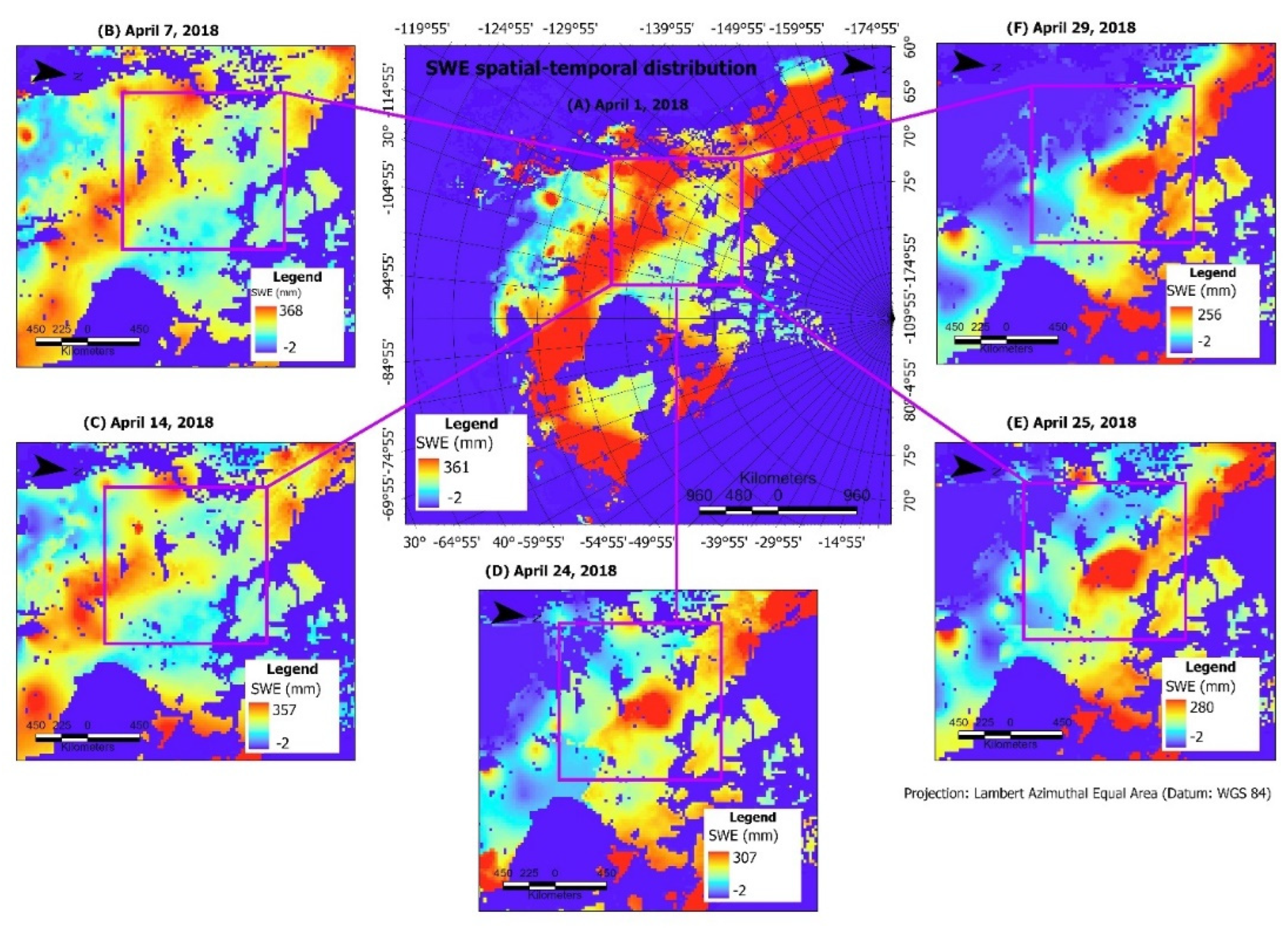
Figure 2.
Siamese Attention U-Net architecture. A sample of labelled SWE data (a) consists of positive (pos) for similar pairs and negative (neg) for dissimilar pairs. The attention gate is depicted in (b), and the integration of the SSIM index into the model’s architecture is shown in (c).
Figure 2.
Siamese Attention U-Net architecture. A sample of labelled SWE data (a) consists of positive (pos) for similar pairs and negative (neg) for dissimilar pairs. The attention gate is depicted in (b), and the integration of the SSIM index into the model’s architecture is shown in (c).
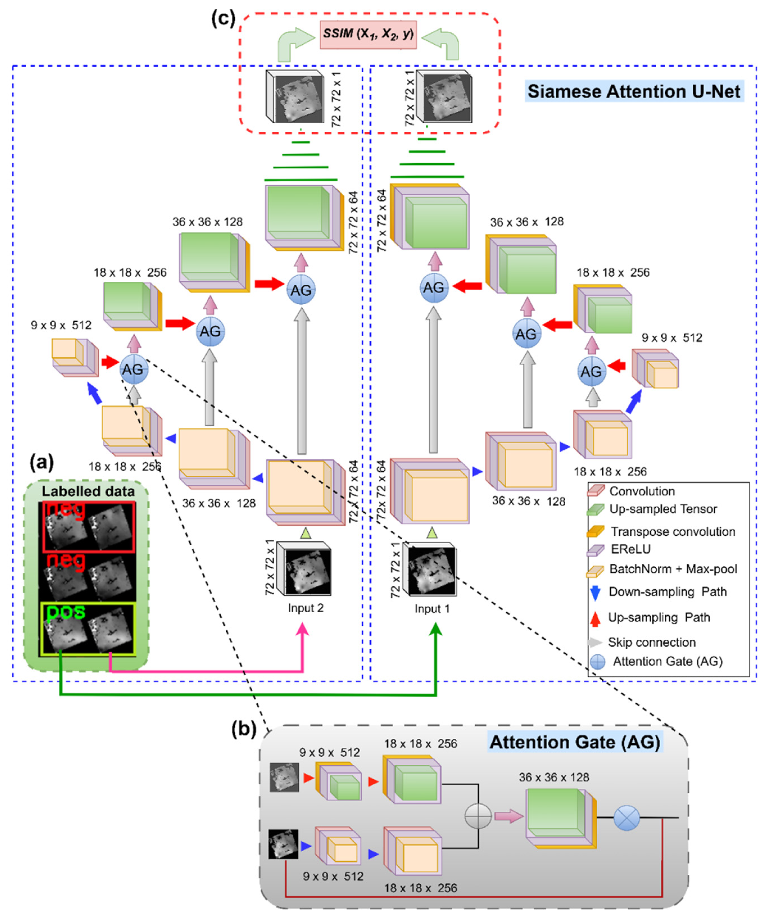
Figure 3.
Frequency of daily SWE change events. The orange line is derived from linear regression conditioned on the frequency of change events over time. The gray is 95% confidence interval.
Figure 3.
Frequency of daily SWE change events. The orange line is derived from linear regression conditioned on the frequency of change events over time. The gray is 95% confidence interval.
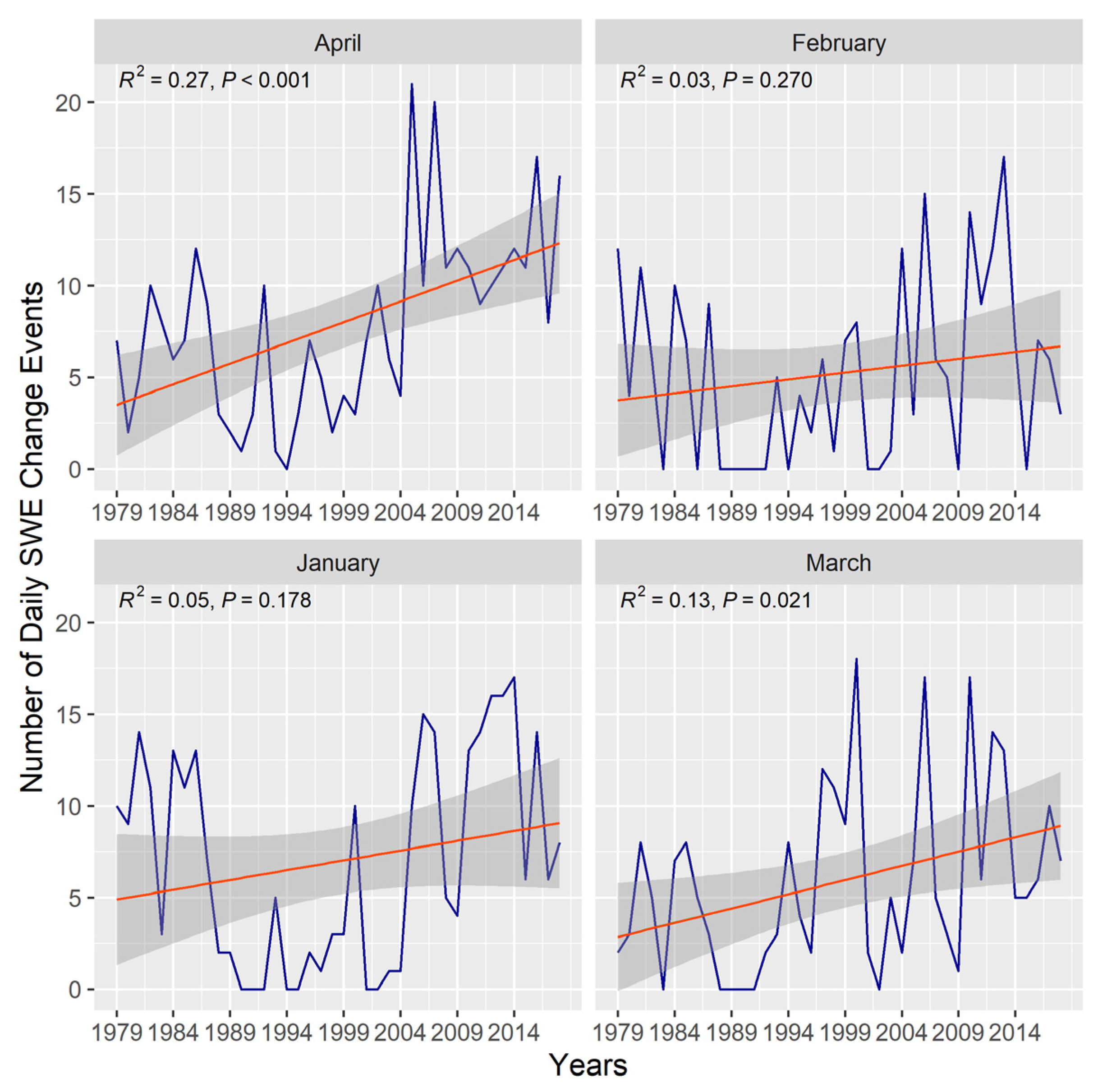
Figure 4.
Mean change points for daily SWE change events. Change segments are represented using red lines. The horizontal width of the lines demarcates change segments.
Figure 4.
Mean change points for daily SWE change events. Change segments are represented using red lines. The horizontal width of the lines demarcates change segments.
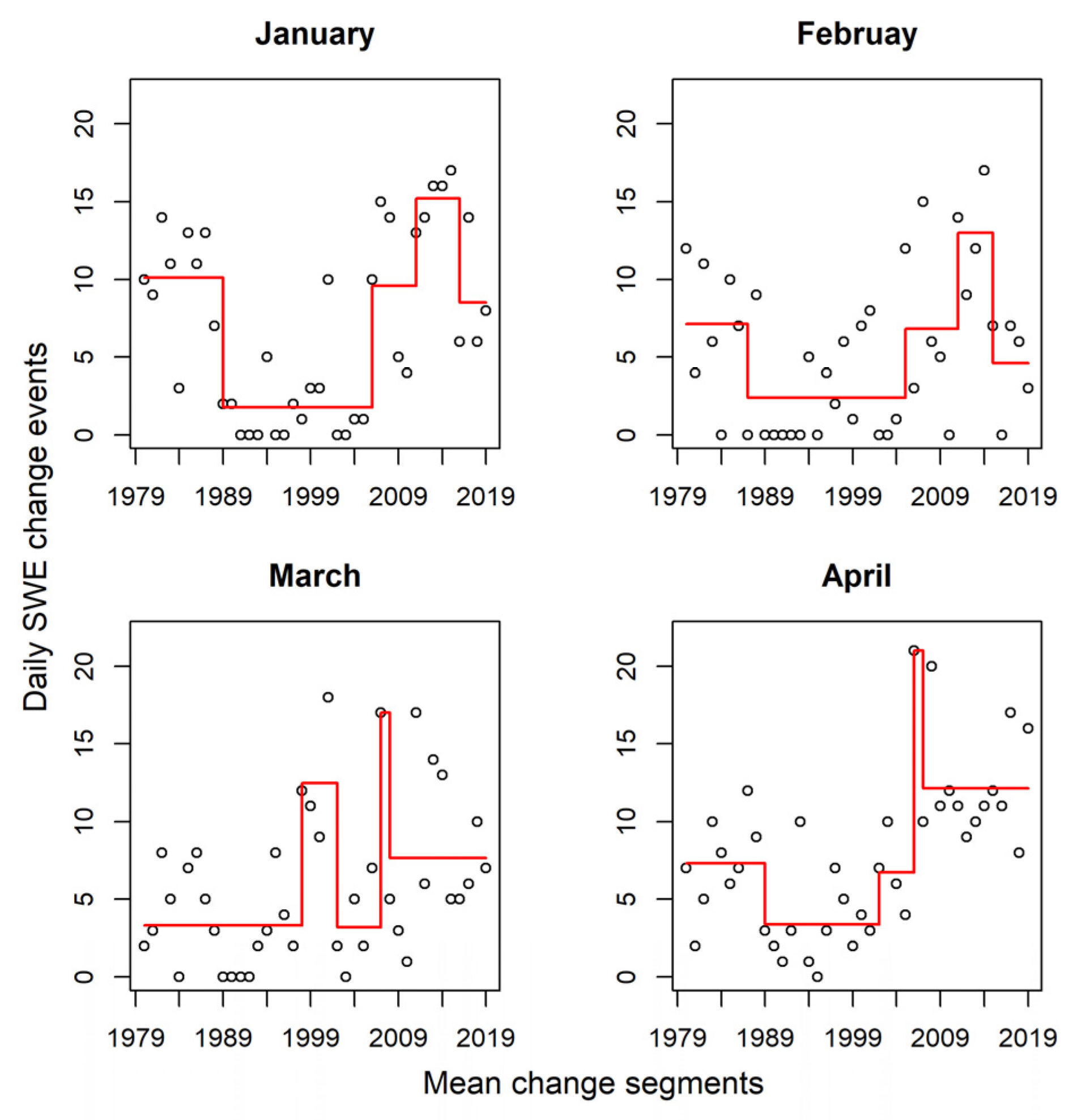
Figure 5.
Northern Hemisphere temperature anomaly mean change segments. The circles represent temperature anomalies, while the red lines denote the mean change segments.
Figure 5.
Northern Hemisphere temperature anomaly mean change segments. The circles represent temperature anomalies, while the red lines denote the mean change segments.
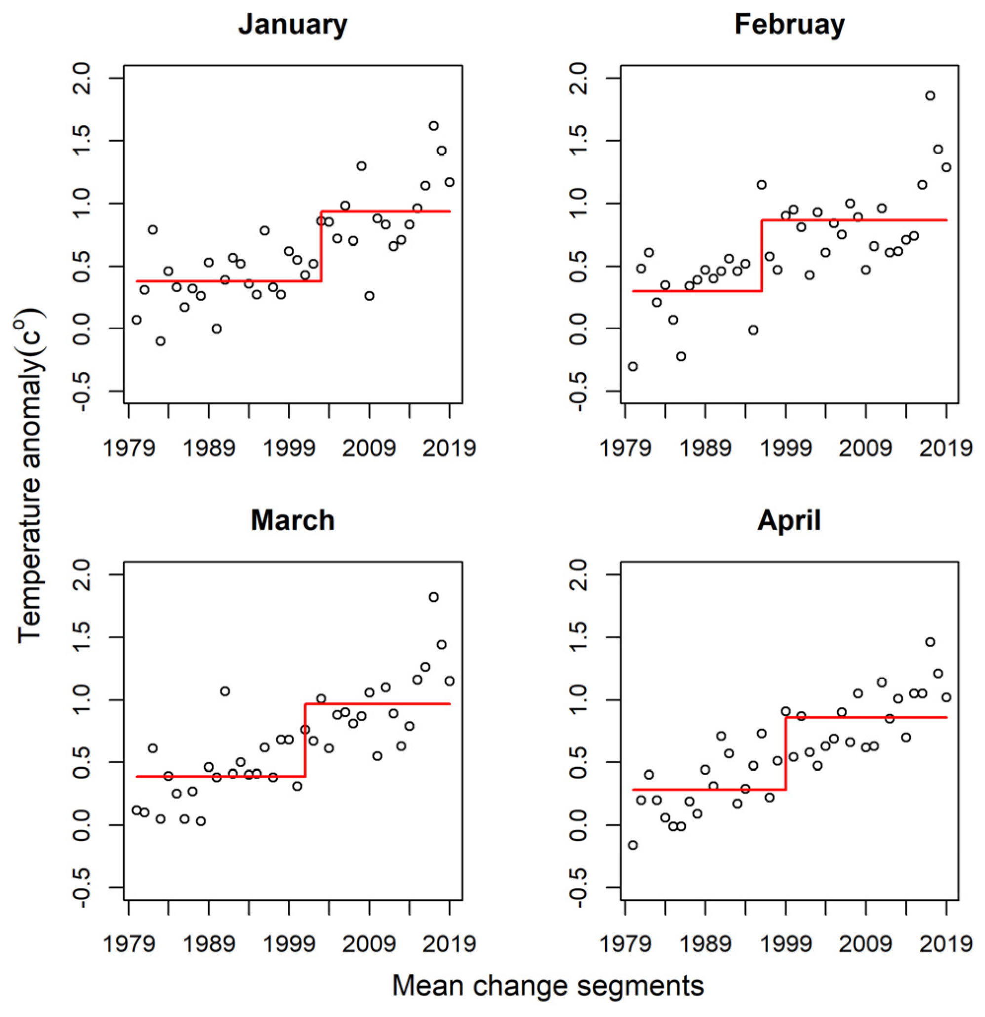
Figure 6.
Northern Hemisphere precipitation anomaly mean change segments. Red lines are used to change segments, while the circles denote precipitation anomalies.
Figure 6.
Northern Hemisphere precipitation anomaly mean change segments. Red lines are used to change segments, while the circles denote precipitation anomalies.
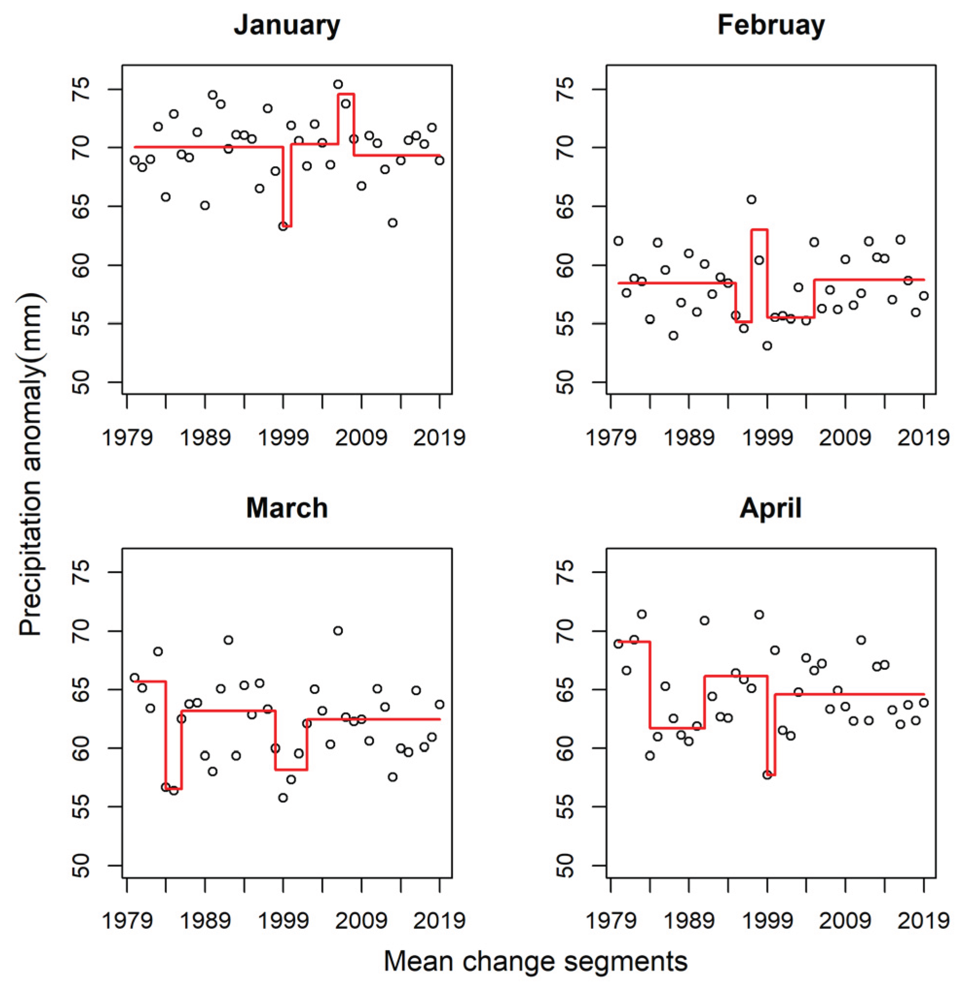

Table 1.
Siamese model’s prediction accuracy.
| Threshold | TPR | FPR | TNR | FNR | PR | F1-score | OA |
|---|---|---|---|---|---|---|---|
| 40% | 100.00 | 100.00 | 0.00 | 0.00 | 30.60 | 0.47 | 30.60 |
| 45% | 100.00 | 37.04 | 62.94 | 0.00 | 54.34 | 70.0 | 74.28 |
| 46% | 100.00 | 12.56 | 87.44 | 0.00 | 77.84 | 88.0 | 91.29 |
| 47% | 100.00 | 3.52 | 96.48 | 0.00 | 92.60 | 96.00 | 97.56 |
| 48% | 100.00 | 0.77 | 99.23 | 0.00 | 98.29 | 99.00 | 99.47 |
| 50% | 98.61 | 0.00 | 100.00 | 1.39 | 100.00 | 99.30 | 99.57 |
Table 2.
Mann-Kendall test and linear regression statistics.
| Month | S | tau | p-Value | R2 |
|---|---|---|---|---|
| January | 7291 | 0.16 | 1.4 ×10⁻¹ | 5.0 ×10⁻² |
| February | 7128 | 0.13 | 2.7 ×10⁻¹ | 3.0 ×10⁻² |
| March | 7275 | 0.25 | 2.6 ×10⁻² | 1.3 ×10⁻¹ |
| April | 7310 | 0.38 | 7.9 ×10⁻⁴ | 2.7 ×10⁻¹ |
Disclaimer/Publisher’s Note: The statements, opinions and data contained in all publications are solely those of the individual author(s) and contributor(s) and not of MDPI and/or the editor(s). MDPI and/or the editor(s) disclaim responsibility for any injury to people or property resulting from any ideas, methods, instructions or products referred to in the content. |
© 2025 by the authors. Licensee MDPI, Basel, Switzerland. This article is an open access article distributed under the terms and conditions of the Creative Commons Attribution (CC BY) license (https://creativecommons.org/licenses/by/4.0/).
Copyright: This open access article is published under a Creative Commons CC BY 4.0 license, which permit the free download, distribution, and reuse, provided that the author and preprint are cited in any reuse.


