
Submitted:
27 October 2025
Posted:
27 October 2025
You are already at the latest version
Abstract
Abstract: Accurate weather prediction plays a vital role in disaster management and minimizing economic losses. This study presents SatNet-B3, a novel lightweight deep learning model for classifying satellite-based weather events with high precision. Built on the EfficientNetB3 backbone with custom classification layers, SatNet-B3 achieved 98.21% accuracy on the LSCIDMR dataset, surpassing existing benchmarks. Ten CNN models, including SatNet-B3, were experimented with to predict eight weather conditions: Tropical Cyclone, Extra-tropical Cyclone, Snow, Low Water Cloud, High Ice Cloud, Vegetation, Desert, and Ocean, with SatNet-B3 yielding the best results. Hyperparameter analysis was conducted to ensure optimal performance. The model addresses challenges like class imbal- ance and inter-class similarity through extensive data preprocessing and augmentation. To support scalability in big data contexts, the pipeline is designed to handle high-resolution geospatial imagery efficiently. Post-training quantization reduced the model size by 90.98% while retaining accuracy. Deployment on a Raspberry Pi 4 achieved a 0.3s inference time, enabling real-time decision-making in edge environments. By integrating explainable AI tools such as LIME and CAM, the model highlights influential image regions, improving interpretability and cognitive situational awareness for intelligent climate monitoring.
Keywords:
satellite imagery
; weather prediction
; edge AI
; deep learning
; explainable AI
1. Introduction
Predicting the weather accurately is crucial for protecting lives and reducing financial damage [15]. Natural disasters like hurricanes, floods, and cyclones have caused huge economic losses worldwide. For example, between 2010 and 2019, hurricanes like Harvey, Irma, and Maria led to about $731 billion in damages [16]. The European Union also reported that extreme weather and climate events caused losses of €738 billion between 1980 and 2023 [17]. Having reliable weather forecasts can help reduce the impact of these disasters by enabling early preparation and more efficient resource management.
Accurate weather forecasting is particularly vital for maritime safety, as it helps sea and ocean travelers to prepare for possible dangers. Reliable weather information helps in planning routes, saving fuel, and reducing the risk of accidents and damage to cargo [18]. However, predicting the weather is challenging due to the complexity of weather patterns. The dynamic nature of atmospheric conditions requires advanced monitoring and prediction technologies to ensure maritime safety. Recent advancements in remote sensing and in-situ measurement platforms have significantly improved weather monitoring systems, leading to better decision-making in maritime operations [19,20]. Microservice-based weather station architectures have also emerged as a scalable and flexible approach for real-time weather data collection and dissemination, addressing the limitations of traditional weather stations [33].
Climate change causes serious effects like loss of life, lower agricultural productivity, and damage to infrastructure. Changes in meteorological, hydrological, and plant physiological conditions, directly impact farming, and further complicates weather prediction efforts [21]. In countries like Bangladesh, accurate weather forecasts are essential for economic stability and public safety. Agriculture, a key part of the economy, relies on weather forecasts to improve crop yields and reduce losses from bad weather. Mobile applications can assist farmers in mitigating the negative impacts of weather phenomena on agricultural production [22]. Similarly, early warnings of cyclones and storms are vital for fishermen who rely on river and coastal systems. Around one million people fish in the southwest coastal region of Bangladesh, an area highly prone to cyclones, sea depression, and tidal surges. Implementing ICT facilities in developing early warning response mechanisms has been shown to enhance the safety and livelihoods of these fishermen [23]. This paper [24] stresses the importance of offering enough warning time for rough sea events through satellite-based weather signals, allowing fishermen to make informed choices to safeguard their lives and livelihoods.
Images from satellite provide significant, real-time insights into varying weather patterns, such as cloud movements, cyclones, and shifts in land coverage. These data streams are a key part of geospatial big data ecosystems and require scalable, intelligent processing pipelines to extract actionable insights [34]. With the proliferation of edge and IoT devices in environmental sensing networks, lightweight, deployable AI models have become increasingly important for on-site, real-time decision-making [35,36]. Satellite-based predictions, coupled with lightweight deployment on edge devices, can provide real-time localized forecasts to remote and resource-limited communities [37]. Recent advancements in satellite imagery and deep learning (DL) have revolutionized weather prediction [7]. By integrating deep learning techniques with satellite data, researchers have developed models capable of accurately classifying weather events. Previous studies have utilized architectures such as CNNs and U-Net models to improve forecasting accuracy [1,2,3,4,5,6]. These studies have greatly improved weather forecasting methods using satellite images. However, most of these existing studies focus on high-performance models without considering their feasibility for big data-driven, edge-based deployment pipelines. These large models often require substantial computational resources, making them impractical for real-time applications in remote or resource-limited settings.
This study proposes SatNet-B3, a novel lightweight CNN-based model designed to accurately predict weather events, classifying eight distinct categories, labeled as Tropical Cyclone, Extratropical Cyclone, Frontal Surface, Westerly Jet, Snow, High Ice Cloud, Low Water Cloud, Ocean, Desert, and Vegetation from satellite imagery. Unlike previous works that emphasize high-capacity deep learning models, SatNet-B3 is optimized for deployment on edge devices while maintaining state-of-the-art accuracy. Our work contributes to the growing field of cognitive computing by enabling real-time intelligent decision-making from satellite data, even in bandwidth- or resource-constrained environments. Our work contributes to the broader field of intelligent edge computing and geospatial analytics by enabling real-time environmental inference under resource constraints. Post-training quantization techniques reduce the model size by 90.98% without significant loss in accuracy. Moreover, this research validates SatNet-B3 on a Raspberry Pi 4 device, achieving an inference time of 0.3 seconds. This confirms its suitability for real-world big data and edge computing applications.
This paper presents the following key contributions:
- A novel edge-deployable, lightweight deep learning model, SatNet-B3, for classifying satellite images from the LSCIDMR dataset, achieving superior performance compared to existing state-of-the-art approaches.
- The application of post-training quantization techniques to significantly reduce model size while maintaining high classification accuracy, enabling real-time inference on embedded and IoT platforms.
- Validation of the model’s inference performance on a Raspberry Pi 4 device, achieving an inference time of 0.3 seconds, demonstrating its efficiency in resource-constrained environments.
The paper is organized into the following sections: Section 2 discusses the existing literature related to this study and its limitations. Section 3 explains the methodology of the system in detail. Evaluation of various classification models is shown in Section 4, and finally, the paper concludes in Section 6.
2. Literature Review
Forecasting weather events accurately plays a critical role for mitigating the impacts of extreme climate events. Traditional methods rely on extensive meteorological data and expert analysis, often requiring significant time and resources. However, recent advancements in deep learning have transformed this field, providing quick and accurate predictions. Techniques such as image segmentation, classification, and edge computing, significantly enhance weather prediction systems. This section will further explore these areas, highlighting the notable literature focusing on these innovative approaches.
2.1. Weather Detection on Local Images
Many recent studies have worked on systems that use local images taken from surroundings with regular cameras for automated weather prediction.
Eden Ship et al. [13] applies Support Vector Machine (SVM) algorithm to classify images for weather conditions in four categories: rainy, low light, haze, and clear. They achieved an accuracy of 92.8% offering computational efficiency against deep learning architectures. However, the dataset is synthetic; the four classes were generated from images of clear weather conditions and is not a real dataset. In the paper by Orestis Papadimitriou et al. [9], a CNN model is introduced to classify weather conditions such as cloudy, sunny, rainy and snowy. The model is trained on collected data that attains an accuracy of 98%.
Saad Minhas et al. [10] uses synthetic data to successfully classify sunny, cloudy, foggy, and rainy images using a virtual simulator. AlexNet, VGGNET, GoogleLeNet, and Residual Network CNNs were experimented upon, where VGGNET had the most efficient accuracy with mAP 0.7334. The study by Yingyue Cao et al. [11], uses a CNN with three convolutional layers and two pooling layers to classify rain, fair weather, tornado, and fog clouds from 4,567 images. The model achieved 90% accuracy for fog and outputs four-channel predictions. The paper [12] introduces MeteCNN, a novel deep CNN model, for classifying 11 weather phenomena with 92% accuracy on the 6,877-image WEAPD dataset. Although these approaches demonstrate strong performance, most operate in controlled or local camera settings and do not address the scalability challenges posed by big geospatial datasets or the need for deployment on edge devices in remote sensing networks.
2.2. Weather Detection on Satellite Imagery
Satellite images are highly effective for real-time prediction on a larger scale. This is necessary for forecasting the weather instantaneously to the people and essentially avoiding and taking precautions against incoming calamities. In big data environments, satellite imagery provides high-volume, high-velocity streams [38] that demand intelligent processing pipelines and cognitive AI models for timely inference [39]. The following works have proposed systems that automate the prediction of weather from satellite images using segmentation and classification-based methods.
2.2.1. Segmentation-Based
In the paper by Songlin Liu et al. [8], a Climate-Award Satellite Images Dataset (CASID) is introduced for land-cover semantic segmentation. The images are categorized into four classes: temperate monsoons, subtropical monsoons, tropical monsoons, and tropical rainforests, from 30 different regions of Asia. The best-achieving model analyzed on their dataset is the SegNeXt model with MSCAN-L backbone, with a mIoU of 63.4% and Dice 76.7%. This study provides a detailed analysis of various semantic segmentation model and unsupervised domain adaptation methods on their CASID dataset. It segments data that are specific to land coverage for detecting monsoon seasons.
A study by Racah E et al. [1] presents a semi-supervised multichannel spatiotemporal CNN model for localization of extreme weather events such as Tropical Depressions, cyclones, extra-tropical cyclones, and atmospheric rivers. Using bounding box predictions with 3D autoencoding CNNS, this model achieved a mean average precision of 52.92 on their curated dataset ExtremeWeather, from CAM5 simulation. However, the data used is a decade older, and the model’s baseline performance may not perform significantly in localizing the climate changes.
Yue Zhao et al. [3] utilize a U-net-based ResNet34 model with a dice coefficient of 0.665 to perform image segmentation for different patterns of clouds such as sugar, flower, fish, and gravel. The data from cloud patterns helps in predicting meteorological disasters. While the Kaggle dataset is quite applicable for weather prediction, it is limited to disasters related to cloud precipitation. Another paper by Sruthy Sebastian et al. [4] predicts cloud types from images of INSAT-3DR satellite with thresholding techniques, edge detection, clustering algorithms, and supervised machine learning algorithms. From their results, Random Forest yielded the highest test accuracy of 90% with PSNR and MSE of 70.13 and 0.00631 respectively. These segmentation approaches provide valuable localized weather insights but often lack optimization for real-time edge-based inference on satellite data streams.
2.2.2. Classification-Based
This paper [2] introduces a snapshot-based residual network, SnapResNet152, that prevents overfitting due to its snapshot ensemble technique and is trained on the LSCIDMR dataset for all 10 classes. Their system analyzes over-fitting and inter-class similarity issues on the imbalanced data. The model performs remarkably with 97.25% classification accuracy but is quite large due to large parameters of the the ResNet152 model.
The study [5] utilizes a dataset from EUMETSAT’s Meteosat-11 satellite which comprises of five satellite products. These products provide meteorological parameters such as cloud height, surface temperature, and humidity profiles. The DeePS at model, based on the Xception architecture, leverages this dataset to predict future satellite images, achieving an average NMAE of 3.84%. It offers faster training and real-time predictions, presenting a simpler alternative to traditional RNN-based models.
Ye Li et al. [6] evaluates deep CNN architectures, including InceptionV3, ResNet50, VGG16, and VGG19, for classifying satellite images into five weather event categories. Using 9081 labeled images from Landsat 8 and Sentinel-2, InceptionV3 achieved the highest accuracy of 92%, outperforming other models in detecting extreme weather events like tropical cyclones, wildfires, and dust storms. While these classification studies have high accuracy, most don’t take into account edge computing limits, real-time smart decision-making, or big data processing, all of which are essential for building scalable and intelligent climate monitoring systems in the real world.

Table 1.
Comparison of Existing Works of Weather Prediction.
| Ref | Year | Dataset | Model | Metrics | Key Features | Limitations |
|---|---|---|---|---|---|---|
| [13] | 2024 | Synthetic (Pascal VOC 2007) | SVM | Acc= 92.8% | Generated images from clear weather conditions, SVM classifier computationally efficient | Synthetic data, limited class variety |
| [8] | 2023 | CASID | SegNeXt | mIoU= 63.4%, Dice= 76.7% | Semantic segmentation, unsupervised domain adaptation methods | Limited to land-coverage data, less significant metrics |
| [1] | 2017 | Extreme-Weather | Multichannel Spatiotemporal CNN | mAP= 52.92% | 3D autoencoding, semi-supervised | Older data, may lack in localizing climate changes |
| [3] | 2020 | Kaggle Cloud Pattern Dataset | U-Net ResNet34 | Dice Coeff= 0.662 | Three loss functions, test-time augmentation | Limited to cloud-related weather forecasts |
| [4] | 2021 | INSAT-3DR | Random Forest | Acc= 90% | Supervised machine learning, edge detection techniques | Limited to cloud-related weather forecasts |
| [2] | 2023 | LSCIDMR | SnapRes-Net152 | Acc= 97.25% | Ensemble architecture, snapshot-based residual network | Large parameters, heavy computations |
| [5] | 2021 | EUMETSAT’s Meteosat-11 satellite images | Custom Xception-based CNN (DeePS at) | NMAE ≈ 3.84% | Short-term nowcasting using multi-channel satellite data, custom CNN model | No reported accuracy on diverse weather patterns |
| [6] | 2021 | NASA, ESA, and NOAA | InceptionV3 | Acc= 92 % | Multiple feature extraction stages | Class Imbalance |
3. Methodology
Figure 1 illustrates the steps taken to implement the proposed model.
3.1. Data Collection
Satellite data related to weather imagery were taken from the LSCIDMR [14] dataset obtained by the Himawari-8 satellite. The original dataset consists of 11 classes: Desert, extratropical cyclone, frontal surface, high ice cloud, low water cloud, ocean, snow, tropical cyclone, vegetation, westerly jet, and label-less. The images are of 104,390 high-resolution (256 × 256) with 10 min temporal resolution and 2km spatial resolution. The dataset has two types of annotations: single (LSCIDMR-S) and multi-label (LSCIDMR-M). The single-label images are simply classified on the major category covering the image, whereas the multi-label images are annotated with segmentations for each class in the image. For this study, LSCIDMR-S is chosen for image classification purposes. There are a total of 40,626 images, excluding the label-less class. However, the classes are highly imbalanced as seen in Figure 2. For this reason, several data preprocessing steps are taken as shown in the following section.
3.2. Data Preprocessing
Initially, the label-less class (63,765 images) was removed as it was insignificant for identifying weather conditions.As observed in Figure 2, there are two classes that have less than 1000 images: Frontal Surface and Westerly Jet. These classes are removed from the dataset to avoid model biasing since they have very few instances. After removing these classes, the dataset is reduced to 39,363 images. Data augmentation techniques are carried out on the reduced dataset to increase the number of samples and, hence, improve model performance and avoid overfitting. Offline augmentation techniques such as horizontal flip, rotation, shear, scale, blur, random brightness, contrast, and zoom are applied, which doubles the dataset to 78,728 images, and Table 3 shows the details of the transformations applied during augmentation. Table 2 shows the distribution of classes in the newly augmented dataset. The number of images in each class has been increased to ensure a large number of samples for training.
Table 2.
Class Distribution After Offline Augmentation.
| Class | Number of Images |
|---|---|
| Tropical Cyclone | 6610 |
| Extra-tropical Cyclone | 9968 |
| Snow | 15262 |
| Low Water Cloud | 3548 |
| High Ice Cloud | 10556 |
| Vegetation | 15662 |
| Desert | 9038 |
| Ocean | 8084 |
| Total | 78728 |
Table 3.
Offline Image Augmentation Transformations.
| Transformations | Setting |
|---|---|
| Horizontal Flip | Applied Randomly |
| Rotation | ±10% |
| Zoom | ±10% |
| Brightness Adjustment | ±10% |
| Random Contrast | ±0.2 |
| Random Brightness | ±0.2 |
| Shear | -10° to +10°, 50% Probability |
| Scale | 0.8 to 1.2, 50% Probability |
Table 4.
Splitting count of each class from the modified dataset.
| Class | Train | Test | Val |
|---|---|---|---|
| Tropical Cyclone | 5288 | 661 | 661 |
| Extra-tropical Cyclone | 7974 | 996 | 998 |
| Snow | 12209 | 1526 | 1527 |
| Low Water Cloud | 2838 | 354 | 356 |
| High Ice Cloud | 8444 | 1055 | 1057 |
| Vegetation | 12529 | 1567 | 1566 |
| Desert | 7230 | 903 | 905 |
| Ocean | 6467 | 808 | 809 |
| Total | 62979 | 7870 | 7879 |
Online augmentation techniques are also applied during the training process, on the train set, to further reduce the impact of overfitting. These techniques include random horizontal flip, rotation, normalization, and resizing to a fixed resolution of 224x224 pixels. The images were normalized by adjusting their pixel values to a scale between 0 and 1, based on the mean and standard deviation for Z-score normalization. This step ensures that the pixel intensity values are standardized, following the equation:
Where x denotes the original feature value prior to normalization. represents the mean (average) of the values in the dataset or feature x, while indicates the standard deviation of the values, reflecting the extent of variation from the mean.
3.3. Training Phase
3.3.1. Model Architecture
SatNet-B3 is a tailored convolutional neural network (CNN) architecture designed for the classification of weather phenomena in high-resolution satellite imagery. It leverages EfficientNetB3 as the backbone, a scalable and efficient CNN framework, with additional custom layers and regularization techniques to enhance performance on an imbalanced and complex weather dataset.
EfficientNetB3 is selected for its ability to balance high accuracy and computational efficiency, making it ideal for processing satellite weather imagery. As shown in Figure 1, the backbone consists of convolutional layers pre-trained on the ImageNet dataset, acting as feature extractors. The final classification layer of the baseline model is removed, allowing the integration of custom layers to refine feature extraction and enhance classification capabilities.
The extracted features from the backbone are passed through a BatchNormalization layer to stabilize training and improve convergence. A GlobalAveragePooling2D layer follows, reducing the spatial dimensions and summarizing the feature maps into a compact vector. This vector is fed into a Dense layer with 256 units and ReLU activation to learn abstract, high-level representations.
To prevent overfitting and improve generalization, a Dropout layer with a 50% rate is added, randomly deactivating neurons during training. The final classification layer consists of a Dense layer with 8 units and a softmax activation function, which outputs a probability distribution over the classes. This streamlined architecture combines pre-trained feature extraction with custom layers to effectively classify weather patterns from satellite images.
3.4. Model Optimization
To enhance the model’s deployment efficiency, post-training quantization was performed, which converted the trained model into TensorFlow Lite (TFLite) format. Two types of optimization techniques were applied: dynamic range INT8 quantization and Float16 quantization. These methods significantly reduced the model’s size and improved inference time while maintaining comparable accuracy, as shown in Table 5.
INT8 Quantization: Dynamic range INT8 quantization involves reducing the precision of weights and activations from 32-bit floating point (FP32) to 8-bit integers (INT8). During inference, most calculations are performed using 8-bit integers. However, the input and output layers are converted back to floating-point values to maintain precision. This approach significantly reduces memory usage and improves computational efficiency, making it ideal for deployment on edge devices. However, the reduction in precision can lead to a slight drop in model accuracy, which is observed in this study with a marginal decrease in accuracy from 98.22% to 98.20%, as shown in Table 5. This trade-off is generally acceptable when the primary goal is memory efficiency and faster inference times, especially for resource-constrained environments.
where W represents the weight values, S is the scale factor, and Z is the zero point. These parameters map the FP32 values to the INT8 range . This approach resulted in a dramatic reduction in model size to 11.6MB, which is a reduction of 90.98% in size and the inference time of 103.51ms, with a negligible drop in accuracy to 98.20%, as indicated in Table 5.
Float16 Quantization Float16 quantization reduces the precision of model weights from FP32 to 16-bit floating-point (FP16) values. Unlike INT8 quantization, FP16 quantization maintains a higher dynamic range and precision for numerical computations, which is particularly advantageous for neural network architectures with sensitive floating-point operations. This method helps preserve model accuracy but does not achieve as significant a reduction in model size as INT8 quantization.
The transformation is expressed as:
where are the original 32-bit floating-point weights, and are the converted 16-bit weights. This technique preserved the model’s accuracy at 98.21% while achieving a smaller model size of 21.3MB and a faster inference time of 74.66ms compared to the original FP32 model, as shown in Table 5.
In this comparison, Float16 offers a good balance between maintaining accuracy and reducing model size, though it is not as memory-efficient as INT8. The trade-off between the two methods—INT8 offering greater memory savings at the cost of a small drop in accuracy, and Float16 preserving accuracy with a lesser reduction in model size—depends on the specific deployment requirements, such as available memory and the criticality of precision in predictions. For highly resource-constrained environments, where model size and inference speed are critical, INT8 quantization is often the preferred choice.
3.5. System Implementation
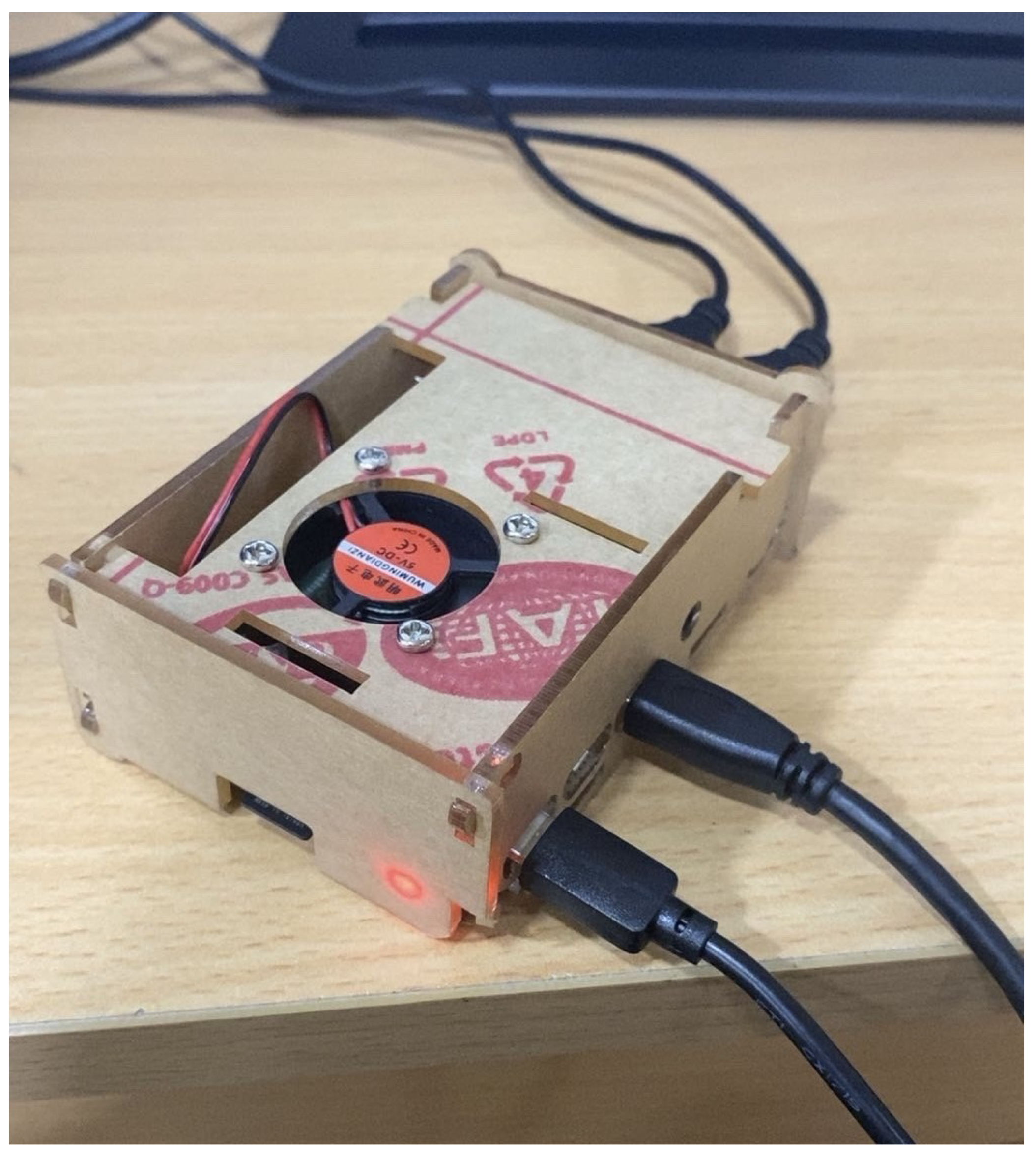
The system is implemented by deploying the quantized SatNet-B3 onto a Raspberry Pi 4 (RPI4) for real-world testing and evaluation. This deployment provides an accurate representation of the model’s performance under actual hardware constraints. With the improved computational capabilities of the RPI4, the model achieved an effective inference time of approximately 300 milliseconds, demonstrating significant efficiency in processing satellite weather imagery. Figure 4shows the actual Raspberry Pi 4 setup used for this deployment.
Figure 3 illustrates the schematic diagram for the Satellite Weather Imagery classification system. The satellite antenna is connected to the Raspberry Pi 4 through the RTL-SDR using a dongle and coaxial cable. The RTL-SDR receives the signals when the satellite passes over and then decodes the image to the RPI4. Consequently, the image is passed to the SatNet-B3 model to classify the predicted weather successfully.
Figure 3.
Schematic Diagram of Satellite Weather Imagery Classification System
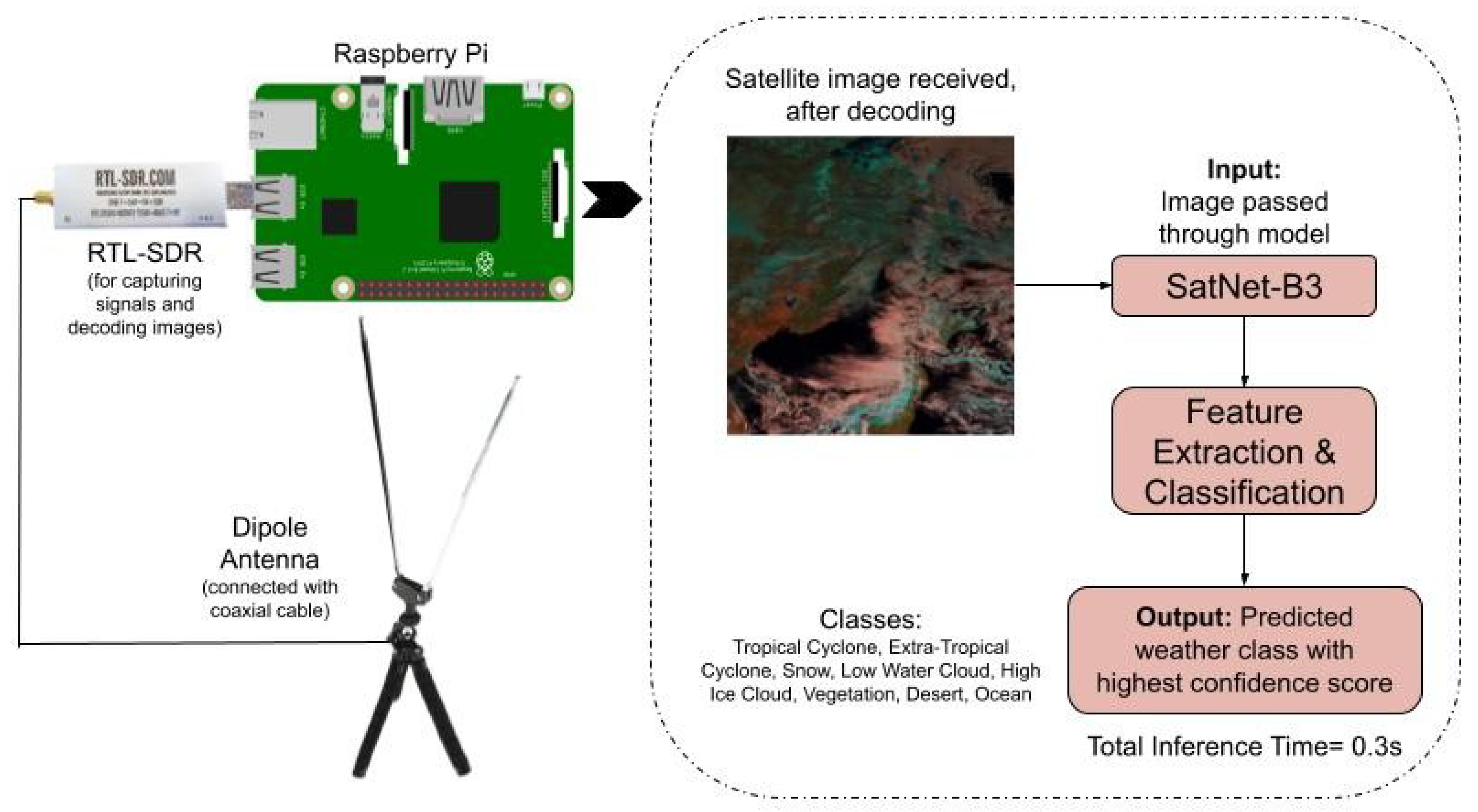
Figure 4.
Raspberry Pi 4 setup used for deployment of the proposed system
3.5.1. Power Consumption
It is important to consider the power requirements of the Raspberry Pi 4 when deploying models like SatNet-B3. Studies have shown that the Raspberry Pi 4 Model B consumes approximately 600 mA (3 W) when idle and up to 1.25 A (6.25 W) under maximum stress with peripherals connected, such as a monitor, keyboard, mouse, and Ethernet [30]. Another study focusing on deep learning applications reported that running convolutional neural networks on a Raspberry Pi can lead to increased power consumption, correlating with model complexity and computational demands [31].
Based on these findings, the power consumption of SatNet-B3 during inference falls within the range of 3 W (idle) to 6.25 W (under load), which is consistent with findings from benchmarking studies on edge devices running deep neural networks [32]. These values highlight the importance of appropriate power provisioning to maintain system stability and performance.
4. Results and Analysis
This section explores the comparative performance of various deep learning models including the proposed model. It illustrates the experimental setup and evaluation criteria used to assess the models, with particular attention to the proposed model’s efficiency and effectiveness.
4.1. Experimental Setting
This section compares the performance of several deep learning models, including the one proposed in this study. It details the experimental setup and evaluation criteria used to assess the models, with a special focus on the efficiency and effectiveness of the proposed model. The experimental setup follows the configuration described in Table 6. Maintaining a consistent environment is important for making a fair and accurate comparison between the models. For model fine-tuning, we used libraries from TensorFlow, as they simplify the process of loading pre-trained weights and provide support for the preprocessing steps required during training.
4.2. Evaluation Metrics
In this study, the following evaluation metrics have been used to assess model performance: Accuracy, Precision, Recall, and F1 Score.
Accuracy quantifies the overall correctness of the model by measuring the proportion of true outcomes (both true positives and true negatives) among all predictions. It is defined as:
where denotes True Positives, denotes True Negatives, denotes False Positives and denotes False Negatives.
Precision focuses on the positive predictions made by the model, indicating the proportion of true positive predictions out of all predicted positives. The formula for precision is:
Recall, also known as Sensitivity, calculates the proportion of true positive results with respect to total actual positives. It is defined as:
Finally, the F1 Score provides a trade-off between Precision and Recall by computing their harmonic mean.
These metrics provide a comprehensive assessment of the model’s performance.
4.3. Achieved Results
In this study, 10 different CNN models were experimented with to evaluate their performance on the task. These models included commonly used architectures as well as the proposed SatNet-B3. Among them, SatNet-B3 delivered the best results, demonstrating superior precision, recall, F1 score, and accuracy compared to the other models. As presented in Table 8, SatNet-B3 achieved a precision of 0.9802, recall of 0.9809, F1 score of 0.9805, and an accuracy of 98.22%. These results show the effectiveness of SatNet-B3 in weather event classification, setting it apart from the other models evaluated.
Table 7.
Comparison of different model architectures
| Model | Precision | Recall | F1 Score | Accuracy | Params (millions) |
|---|---|---|---|---|---|
| ResNet50V2 | 0.9686 | 0.9573 | 0.9625 | 96.66 | 25.6 |
| ResNet101 | 0.9413 | 0.9400 | 0.9394 | 94.48 | 44.7 |
| MobileNetV2 | 0.9444 | 0.9422 | 0.9428 | 94.71 | 3.5 |
| DenseNet121 | 0.9583 | 0.9513 | 0.9544 | 95.71 | 8.1 |
| DenseNet201 | 0.9647 | 0.9585 | 0.9610 | 96.45 | 20.2 |
| Xception | 0.9636 | 0.9672 | 0.9653 | 96.74 | 22.9 |
| InceptionV3 | 0.9644 | 0.9661 | 0.9652 | 96.70 | 23.9 |
| InceptionResNetV2 | 0.9214 | 0.9133 | 0.9136 | 91.04 | 55.9 |
| NASNetMobile | 0.9249 | 0.9026 | 0.9111 | 91.33 | 5.3 |
| SatNet-B3 | 0.9802 | 0.9809 | 0.9805 | 98.22 | 12.3 |
The confusion matrix in Figure 5 shows the number of correctly identified instances in the diagonal values. All of the eight classes represent strong classification. Some minor misclassification trends can be seen, such as Desert having 16 instances of misclassification with Vegetation, and Snow having 13 instances with Desert. This can be due to being visually similar, and improvements can made by collecting more samples of underrepresented classes.
The ROC (Receiver Operating Characteristic) curve in Figure 6 plots the True Positive Rate against the False Positive Rate. Curves of models across its base, Float16, and INT8 formats have been compared, denoting a good AUC value. Figure 7 represent the trade-off between precision and recall with the AUC greater than 0.99 among all classes.
The performance curves in Figure 8 show the trend of the training and validation accuracy and loss. The accuracy curves converge near 98%, which suggests that the model has learned well. The decreasing trend of the loss curves shows that the model is training effectively.
4.4. Ablation Studies
To assess the impact of the custom layers added to the EfficientNetB3 backbone, an ablation study was conducted by progressively adding components and evaluating their performance. The results, shown in Table 8, demonstrate the effectiveness of each layer combination.
Starting with the baseline model (EB + TLF + GAP + Dense:8), where the trainable layers are frozen, the performance is relatively limited. Unfreezing the layers (EB + TLU + GAP + Dense:8) improves the model’s flexibility, resulting in better performance. Further enhancement is observed with the addition of an extra Dense layer (EB + TLU + GAP + Dense:256 + Dense:8), which refines feature extraction, achieving an accuracy of 97.83%.
The inclusion of Batch Normalization (BN) and an extra Dense layer (EB + TLU + GAP + BN + Dense:256 + Dense:8) yields the best results, achieving a precision of 98.02%, recall of 98.09%, and an accuracy of 98.22%. These findings confirm that this particular combination of custom layers, significantly enhance model performance by stabilizing training and improving convergence. The study highlights the importance of these modifications in optimizing the model’s classification capability.
Table 8.
Comparison of model architectures and their performance. EB: EfficientNetB3 Base, TLF: Trainable Layers Frozen, TLU: Trainable Layers Unfreeze, GAP: Global Average Pooling Layer, Dense: Dense Layer, BN: Batch Normalization Layer
Table 8.
Comparison of model architectures and their performance. EB: EfficientNetB3 Base, TLF: Trainable Layers Frozen, TLU: Trainable Layers Unfreeze, GAP: Global Average Pooling Layer, Dense: Dense Layer, BN: Batch Normalization Layer
| Model | Precision | Recall | F1 Score | Accuracy |
|---|---|---|---|---|
| EB + TLF + GAP + Dense:8 | 0.8381 | 0.8238 | 0.8288 | 0.8505 |
| EB + TLU + GAP + Dense:8 | 0.9315 | 0.8954 | 0.9078 | 0.9192 |
| EB + TLU + GAP + Dense:256 + Dense:8 | 0.9760 | 0.9762 | 0.9761 | 0.9783 |
| EB + TLU + GAP + BN + Dense:256 + Dense:8 | 0.9802 | 0.9809 | 0.9805 | 98.22 |
4.5. Hyperparameter Analysis
The hyperparameter analysis process for the model focused on adjusting several key parameters, such as the optimizer, learning rate, and batch size. Table 9 provides a summary of the performance metrics, including accuracy and F1 score, for various optimizers and their corresponding parameter configurations. Among the optimizers tested, the Adam optimizer with a learning rate of 0.0005 and a batch size of 16 achieved the best performance, yielding an accuracy of 0.9822 and an F1 score of 0.9805. The results suggest that the selected combination of parameters for the Adam optimizer outperforms other optimizers such as Adadelta, SGD, RMSprop, and AdaGrad, as highlighted in the table. This analysis indicates that fine-tuning the hyperparameters is crucial for achieving optimal model performance in classifying satellite-based weather events.
Table 9.
Hyperparameter Analysis
| Optimizer | Learning Rate | Batch Size | Accuracy | F1 |
|---|---|---|---|---|
| Adam | 0.0005 | 16 | 0.9822 | 0.9805 |
| Adadelta | 0.001 | 32 | 0.7487 | 0.7271 |
| SGD | 0.005 | 16 | 0.9438 | 0.9392 |
| RMSprop | 0.0001 | 32 | 0.9799 | 0.9784 |
| AdaGrad | 0.01 | 32 | 0.9732 | 0.9716 |
4.6. Explainable AI
Explainable AI (XAI) has emerged in response to the increasing reliance on black-box models, making their decision-making more transparent. It includes various techniques that enhance the clarity and reliability of machine-learning models, ensuring their outputs are comprehensible to humans. In image classification, it examines whether the model prioritizes meaningful regions, aligning with human perception. Common approaches for this include LIME and CAM.
4.6.1. LIME
LIME (Local Interpretable Model-Agnostic Explanations) is a technique that enhances model interpretability by providing explanations for individual predictions. It is model-agnostic, meaning it can be applied to any supervised regression or classification model. LIME supports various data types, including images, text, and tabular data, making it a versatile tool for understanding machine-learning decisions.[25,26]
4.6.2. CAM
Class Activation Mapping (CAM) is an explainability technique used in convolutional neural networks (CNNs) to highlight image regions which are most relevant to a model’s prediction. By generating heatmaps, CAM helps visualize which features contribute to classification decisions, improving interpretability. [29]
In disaster image detection, CAM has been proved useful in detecting the most significant areas damaged by natural disasters, allowing for more transparent and trustworthy damage assessment. Its ability to highlight crucial regions guarantees that model judgments are consistent with human expert analysis, which increases trust in AI-powered disaster response systems. [27,28]
4.6.3. Model Interpretability Using XAI
In this study, explainable AI techniques such as CAM and LIME were used to provide visual explanations for the model’s predictions. LIME highlights the edges that influenced the decision, while CAM generates heatmaps to indicate the key regions the model focused on. These techniques highlight the important features that influenced the model’s decision, showing that the predictions are based on the right regions of the image, as shown in Figure 9.
4.7. Further Validation
The robustness and generalization capability of the proposed model is further examined by evaluating its performance on data with varying brightness levels and blurred images. A detailed discussion of the evaluation results for each method is provided in the following sections.
4.7.1. Brightness Adjustment
The model’s robustness to varying lighting conditions was evaluated by adjusting the brightness of the test images by ±20%. Despite these changes, the model retained 99% accuracy on both brighter and darker images, demonstrating its strong generalization ability under different illumination levels. Table 10 shows the accuracies achieved by the model with brightness adjustments, and Figure 10 presents examples of the images used in this evaluation, highlighting the variations in brightness.
4.7.2. Blurred Image Evaluation
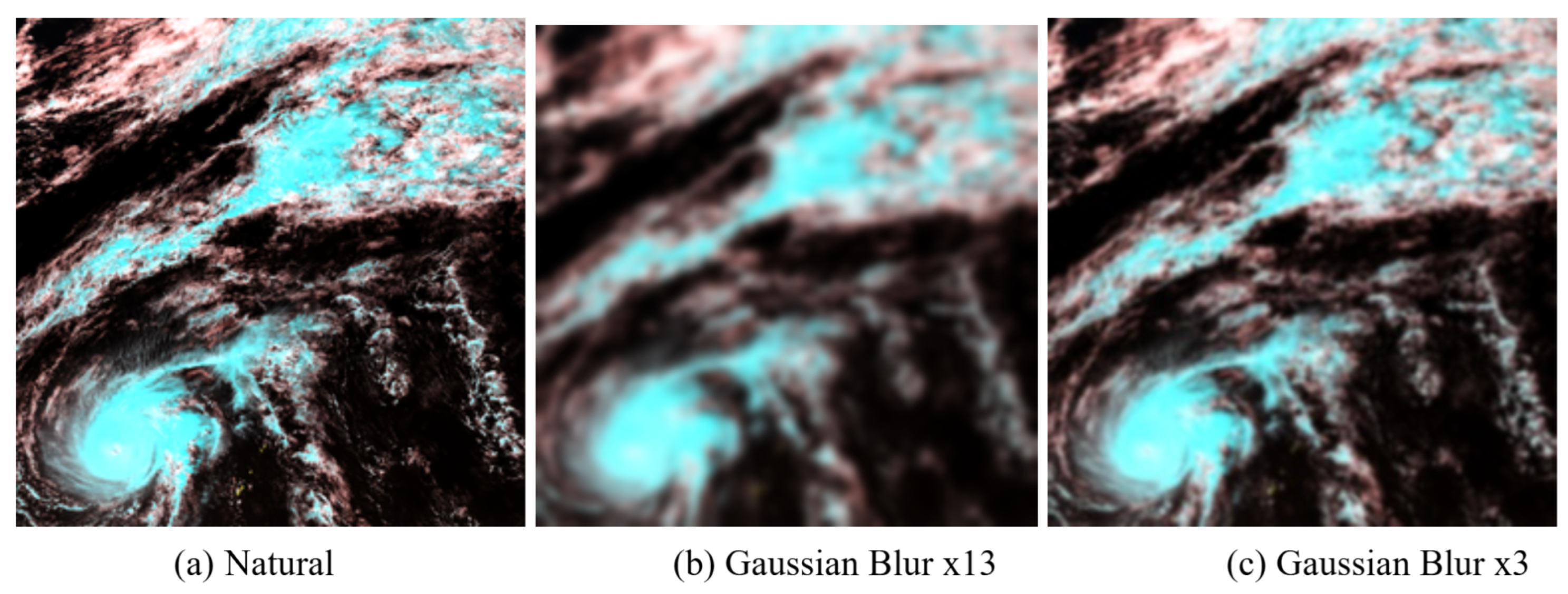
The model’s ability to handle blurred inputs was assessed by evaluating its performance on images with varying levels of blur. Despite increasing blur intensity, the model maintained high accuracy, which demonstrates its robustness to image degradation. Table 11 presents the accuracies achieved under different blur levels.
Figure 11.
Varying Intensity of Blurred Image.
5. Discussion
Table 12 presents a comparative analysis of recent works in weather prediction using satellite imagery. Among these, the current state-of-the-art (SOTA) approach [2] utilized a snapshot-based residual network, SnapResNet152, achieving an accuracy of 97.25% on the LSCIDMR dataset. This dataset, as introduced in [14], also explored several architectures, including AlexNet, VGG-Net-19, ResNet-101, and EfficientNet, with an average accuracy of 92.475%, establishing a baseline for future work in weather prediction using satellite imagery. Despite the strong performance of prior architectures, including the SOTA SnapResNet152, the proposed SatNet-B3 model surpasses these benchmarks, achieving an accuracy of 98.21% and establishing a new standard in weather prediction using satellite imagery.
This improvement underscores the capability of the developed technique to classify high-resolution satellite images with enhanced precision, even under challenging conditions. By using the EfficientNetB3 backbone along with custom classification layers, SatNet-B3 effectively captures and extracts significant features from complex weather patterns, allowing it to distinguish between similar classes with greater accuracy. In addition, comprehensive data preprocessing and augmentation techniques were implemented to address the challenges posed by class imbalance and to enhance model generalization. Offline augmentation methods were used which was complemented by online augmentation during training, which further reduced the risk of overfitting and improved the model’s robustness against diverse weather scenarios.
Furthermore, the lightweight nature of SatNet-B3 distinguishes it from prior works. While many existing methods, including SnapResNet152 [2], prioritize maximizing accuracy without considering deployment constraints, SatNet-B3 introduces a practical edge-oriented approach. Post-training quantization techniques, such as INT8 and Float16 quantization, were applied, which significantly reduced the model’s size and improved inference time, making it highly suitable for deployment on edge devices in resource-constrained environments. The model was also successfully deployed on a Raspberry Pi 4 device, where it achieved an inference time of 0.3 seconds. This real-world deployment validates the model’s efficiency and demonstrates its feasibility for practical applications in edge-based meteorological systems.
Beyond its technical performance, this study emphasizes the interpretability of the model, which is important for meteorological applications. Explainable AI methods like LIME and Class Activation Mapping (CAM) were applied to show which parts of the satellite images had the most impact on the model’s predictions. This capability enhances the model’s reliability, particularly for critical scenarios like disaster management and agricultural planning.
Overall, the results demonstrate that SatNet-B3 not only surpasses the SOTA accuracy achieved by SnapResNet152 but also addresses key limitations of prior works by effectively balancing performance, interpretability, and deployability. Its ability to handle high inter-class similarity and class imbalance while being optimized for lightweight deployment positions it as a robust solution for satellite-based weather prediction.
6. Conclusions
Accurately predicting weather events is critical for disaster management and mitigating economic losses. This study introduced SatNet-B3, a lightweight deep learning architecture designed for high-precision classification of satellite-based weather phenomena. It utilized the EfficientNetB3 as backbone with custom classification layers and SatNet-B3 achieved a state-of-the-art accuracy of 98.21% on the LSCIDMR dataset, surpassing the existing benchmarks. The model was further enhanced through comprehensive data preprocessing and augmentation methods, effectively addressing challenges like class imbalance and high inter-class similarity. To optimize deployment feasibility, post-training quantization techniques, including INT8 and Float16 formats, were applied, reducing the model size and inference time. The successful deployment of SatNet-B3 on a Raspberry Pi 4 device, where it achieved an inference time of 0.3 seconds, validates its suitability for real-world applications in resource-constrained settings. Explainable AI techniques, such as LIME and Class Activation Mapping (CAM), were used to show the areas in satellite images that had the most impact on the model’s predictions. This improves the model’s interpretability and enhances its reliability, particularly for critical meteorological applications.
While SatNet-B3 demonstrates strong potential for weather prediction, it can still be further explored. Future work could involve expanding the system’s deployment to integrate physical antenna systems for direct real-time data acquisition, further enhancing its practical applicability. Additionally, the model could be tested on various edge devices beyond the Raspberry Pi 4 to assess environment-specific performance. Deployment of the system on boats or ships for real-time data collection and weather prediction could greatly improve safety and preparedness for sea travelers. The model can also be tested on other edge or hardware devices for environment-specific uses and can be integrated with live-weather systems in disaster-prone regions for more accurate analysis. Furthermore, evaluating the model on data from different satellites can further improve its generalizability. This research has the potential to improve weather prediction systems and enhance disaster preparedness in resource-limited settings.
Funding
This research received no external funding
Author Contributions: Tarbia Hasan
: Methodology, Data curation, Investigation, Validation, Visualization, Writing- Original Draft, Formal analysis, Writing- Review & Editing Jareen Anjom: Methodology, Data curation, Investigation, Validation, Visualization, Writing- Original Draft, Formal analysis, Writing- Review & Editing Zia Ush Shamszaman: Supervision, Project Administration, Validation, Writing- Review & Editing, Formal analysis. Md. Ishan Arefin Hossain: Conceptualization, Supervision, Project Administration, Validation, Writing- Review & Editing, Formal analysis.
Institutional Review Board Statement
Not applicable
Informed Consent Statement
Not applicable
Data Availability Statement
The dataset utilized in this study, LSCIDMR (Large-Scale Satellite Cloud Image Database for Meteorological Research), is publicly available and can be accessed via the following GitHub repository: https://github.com/Zjut-MultimediaPlus/LSCIDMR
Conflicts of Interest
The authors declare no conflicts of interest.
References
- Racah, E.; Beckham, C.; Maharaj, T.; Kahou, S.E.; Prabhat; Pal, C. ExtremeWeather: A large-scale climate dataset for semi-supervised detection, localization, and understanding of extreme weather events. arXiv.org 2016, https://arxiv.org/abs/1612.02095.
- Yousaf, R.; Rehman, H.Z.U.; Khan, K.; Khan, Z.H.; Fazil, A.; Mahmood, Z.; Qaisar, S.M.; Siddiqui, A.J. Satellite Imagery-Based Cloud Classification using Deep Learning. Remote Sens. 2023, 15, 5597. [Google Scholar] [CrossRef]
- Zhao, Y.; Shangguan, Z.; Fan, W.; Cao, Z.; Wang, J. U-Net for Satellite Image Segmentation: Improving the Weather Forecasting. In Proceedings of the 2020 5th International Conference on Universal Village (UV); 2020; pp. 1–6. [Google Scholar] [CrossRef]
- Sebastian, S. ; Sutha Lakshmi, Kumar, P.; Annadurai. Segmentation of satellite images using machine learning algorithms for cloud classification. 2021.
- Ionescu, V.-S.; Czibula, G.; Mihuleţ, E. DeePS at: A deep learning model for prediction of satellite images for nowcasting purposes. Procedia Comput. Sci. 2021, 192, 622–631. [Google Scholar] [CrossRef]
- Li, Y.; Momen, M. Detection of weather events in optical satellite data using deep convolutional neural networks. Remote Sens. Lett. 2021, 12, 1227–1237. [Google Scholar] [CrossRef]
- Ren, X.; Li, X.; Ren, K.; Song, J.; Xu, Z.; Deng, K.; Wang, X. Deep learning-based weather prediction: A survey. Big Data Res. 2020, 23, 100178. [Google Scholar] [CrossRef]
- Liu, S.; Chen, L.; Zhang, L.; Hu, J.; Fu, Y. A large-scale climate-aware satellite image dataset for domain adaptive land-cover semantic segmentation. ISPRS J. Photogramm. Remote Sens. 2023, 205, 98–114. [Google Scholar] [CrossRef]
- Papadimitriou, O.; Kanavos, A.; Mylonas, P.; Maragoudakis, M. Advancing Weather Image Classification Using Deep Convolutional Neural Networks. In Proceedings of the 2023 18th International Workshop on Semantic and Social Media Adaptation &, 2023, Personalization (SMAP); pp. 1–6. [CrossRef]
- Minhas, S.; Khanam, Z.; Ehsan, S.; McDonald-Maier, K.; Hernández-Sabaté, A. Weather Classification by Utilizing Synthetic Data. Sensors 2022, 22, 3193. [Google Scholar] [CrossRef] [PubMed]
- Cao, Y.; Yang, H. Weather prediction using cloud’s images. In Proceedings of the 2022 International Conference on Big Data, Information and Computer Network (BDICN), Sanya, China; 2022; pp. 820–823. [Google Scholar] [CrossRef]
- Xiao, H.; Zhang, F.; Shen, Z.; Wu, K.; Zhang, J. Classification of weather phenomena from images by using deep convolutional neural network. Earth Space Sci. 2021, 8, 1. [Google Scholar] [CrossRef]
- Ship, E.; Spivak, E.; Agarwal, S.; Birman, R.; Hadar, O. Real-Time Weather Image Classification with SVM. arXiv, 2024. https://arxiv.org/abs/2409.00821.
- Bai, C.; Zhang, M.; Zhang, J.; Zheng, J.; Chen, S. LSCIDMR: Large-scale satellite cloud image database for meteorological research. IEEE Trans. Cybern. 2021, 52, 12538–12550. [Google Scholar] [CrossRef] [PubMed]
- Shen, D.; Zuo, Z.; Zhang, X.; Zhao, X. The impact of weather forecast accuracy on the economic value of weather-sensitive industries. 2023. [CrossRef]
- Allianz. Cyclones: Economic losses and impact on the global economy. Allianz, 2024. https://www.allianz.com/content/dam/onemarketing/azcom/Allianz_com/economic-research/publications/specials/en/2024/october/2024-10-09-Cyclones-AZ.pdf.
- European Environment Agency. Economic losses from climate-related extremes in Europe. European Environment Agency, 2023. https://www.eea.europa.eu/en/analysis/indicators/economic-losses-from-climate-related.
- Toroman, A. 10 reasons why you should be using maritime weather forecasts. https://spire.com/blog/maritime/10-reasons-why-you-should-be-using-maritime-weather-forecasts/.
- Kadhafi, M. Maritime safety in the digital era as the role of weather monitoring and prediction technology. Maritime Park J. Maritime Technol. Soc. 2024, 3, 28–33. [Google Scholar] [CrossRef]
- Smit, P.B.; Houghton, I.A.; Jordanova, K.; Portwood, T.; Shapiro, E.; Clark, D.; Sosa, M.; Janssen, T.T. Assimilation of distributed ocean wave sensors. arXiv, 2003. [Google Scholar]
- Gornall, J.; Betts, R.; Burke, E.; Clark, R.; Camp, J.; Willett, K.; Wiltshire, A. Implications of climate change for agricultural productivity in the early twenty-first century. Philos. Trans. R. Soc. Lond., B, Biol. Sci. 2010, 365, 2973–2989. [Google Scholar] [CrossRef] [PubMed]
- Khan, M.N.; Farukh, M.; Rahman, M. Application of weather forecasting apps for agricultural development in Bangladesh. 2018. [CrossRef]
- Give2Asia. Promoting ICT facilities in developing early warning response mechanisms for cyclone-exposed seagoing fishers in southwest Bangladesh. https://give2asia.org/promoting-ict-facilities-in-developing-early-warning-response-mechanisms-for-cyclone-exposed-seagoing-fishers-in-southwest-bangladesh.
- Elrha. A people-centered early warning system specifically designed to address the needs of selected fishing communities in Cox’s Bazaar. https://www.elrha.org/project/people-centered-early-warning-system-specifically-designed-address-needs-selected-fishing-communities-coxs-bazaar.
- Garreau, D.; Von Luxburg, U. Explaining the Explainer: A First Theoretical Analysis of LIME. arXiv, 2020. https://arxiv.org/abs/2001.03447.
- Ribeiro, M.T.; Singh, S.; Guestrin, C. "Why Should I Trust You?": Explaining the Predictions of Any Classifier. arXiv, 2016. https://arxiv.org/abs/1602.04938.
- Franceschini, R.G.; Liu, J.; Amin, S. Damage Estimation and Localization from Sparse Aerial Imagery. arXiv, 2021. https://arxiv.org/abs/2111.03708.
- Chen, T.Y. Interpretability in Convolutional Neural Networks for Building Damage Classification in Satellite Imagery. arXiv, 2022. https://arxiv.org/abs/2201.10523.
- Zhou, B.; Khosla, A.; Lapedriza, A.; Oliva, A.; Torralba, A. Learning Deep Features for Discriminative Localization. arXiv, 2015. https://arxiv.org/abs/1512.04150.
- Raspberry, Pi. In Wikipedia, 2025. https://en.wikipedia.org/wiki/Raspberry_Pi.
- Tang, R.; Wang, W.; Tu, Z.; Lin, J. An Experimental Analysis of the Power Consumption of Convolutional Neural Networks for Keyword Spotting. arXiv, 2017. https://arxiv.org/abs/1711.00333.
- Baller, S.P.; Jindal, A.; Chadha, M.; Gerndt, M. DeepEdgeBench: Benchmarking Deep Neural Networks on Edge Devices. arXiv, 2021. https://arxiv.org/abs/2108.09457.
- Bonilla, J.; Carballo, J.; Abad-Alcaraz, V.; Castilla, M.; Álvarez, J.; Fernández-Reche, J. A real-time and modular weather station software architecture based on microservices. Environ. Model. Softw. 2025, 186, 106337. [Google Scholar] [CrossRef]
- Li, S.; Dragicevic, S.; Castro, F.A.; Sester, M.; Winter, S.; Coltekin, A.; Pettit, C.; Jiang, B.; Haworth, J.; Stein, A.; Cheng, T. Geospatial big data handling theory and methods: A review and research challenges. ISPRS J. Photogramm. Remote Sens. 2015, 115, 119–133. [Google Scholar] [CrossRef]
- Yang, R.; Chen, Z.; Wang, B.; Guo, Y.; Hu, L. A lightweight detection method for remote sensing images and its Energy-Efficient accelerator on edge devices. Sensors 2023, 23, 6497. [Google Scholar] [CrossRef] [PubMed]
- Wei, J.; Cao, S. Application of edge intelligent computing in satellite Internet of Things. In Proceedings of the 2019 IEEE International Conference on Smart Internet of Things (SmartIoT); 2019; pp. 85–91. [Google Scholar] [CrossRef]
- Boucetta, A.Y.; Baziz, M.; Hamdad, L.; Allal, I. Optimizing for Edge-AI based satellite image processing: A survey of techniques. In Proceedings of the 2024 IEEE Mediterranean and Middle-East Geoscience and Remote Sensing Symposium (M2GARSS); 2024; pp. 83–87. [Google Scholar] [CrossRef]
- Dritsas, E.; Trigka, M. Remote Sensing and Geospatial Analysis in the Big Data Era: A Survey. Remote Sens. 2025, 17, 550. [Google Scholar] [CrossRef]
- Nguyen, D.; Le, H. A. A Big Data Framework for Satellite Images Processing Using Apache Hadoop and RasterFrames: A Case Study of Surface Water Extraction in Phu Tho, Viet Nam. Int. J. Adv. Comput. Sci. Appl. 2020, 11, 89–94. [Google Scholar] [CrossRef]
Figure 1.
Overview of the proposed method.
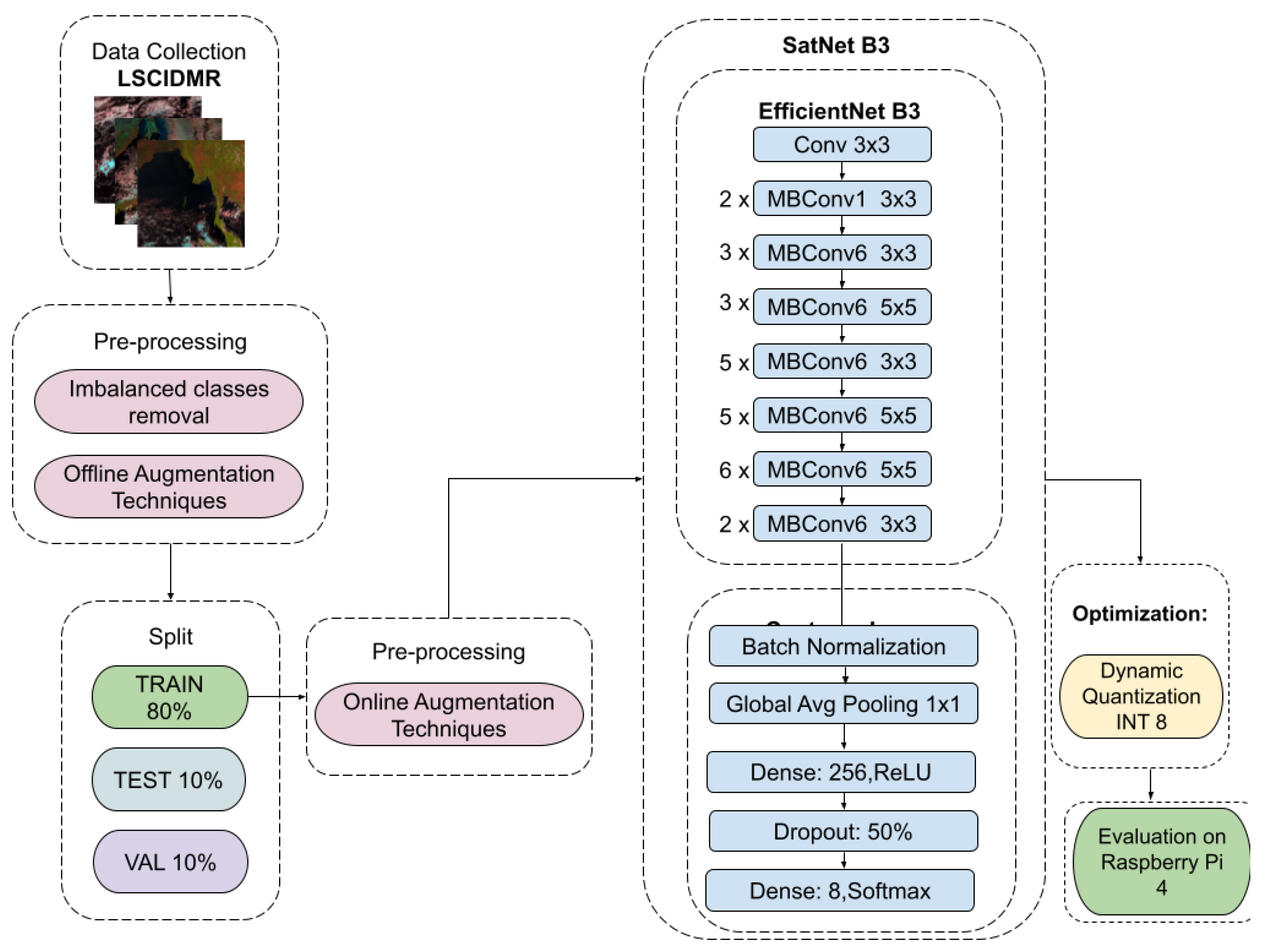
Figure 2.
Original Class Distribution
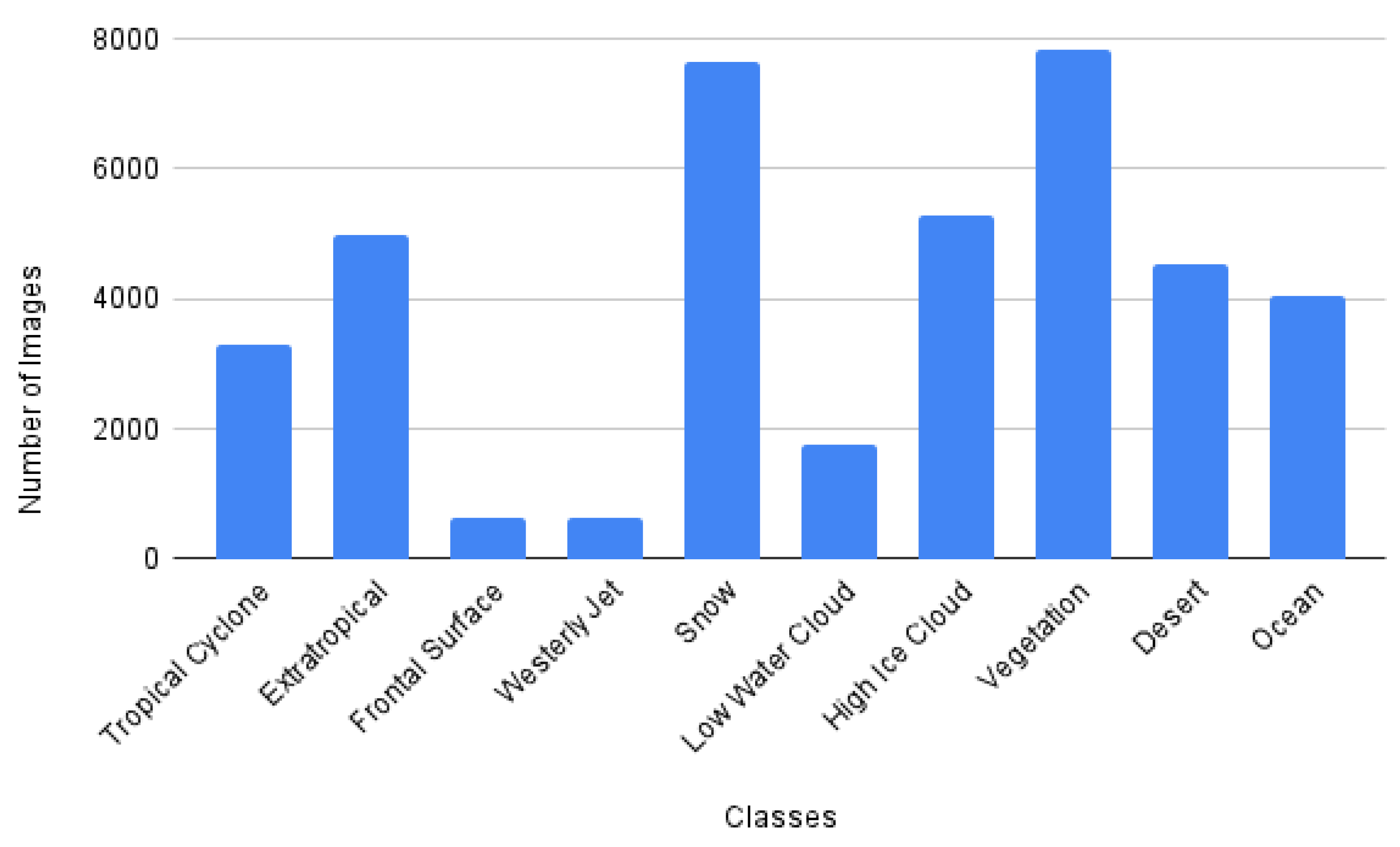
Figure 5.
Confusion Matrix of SatNet-B3.
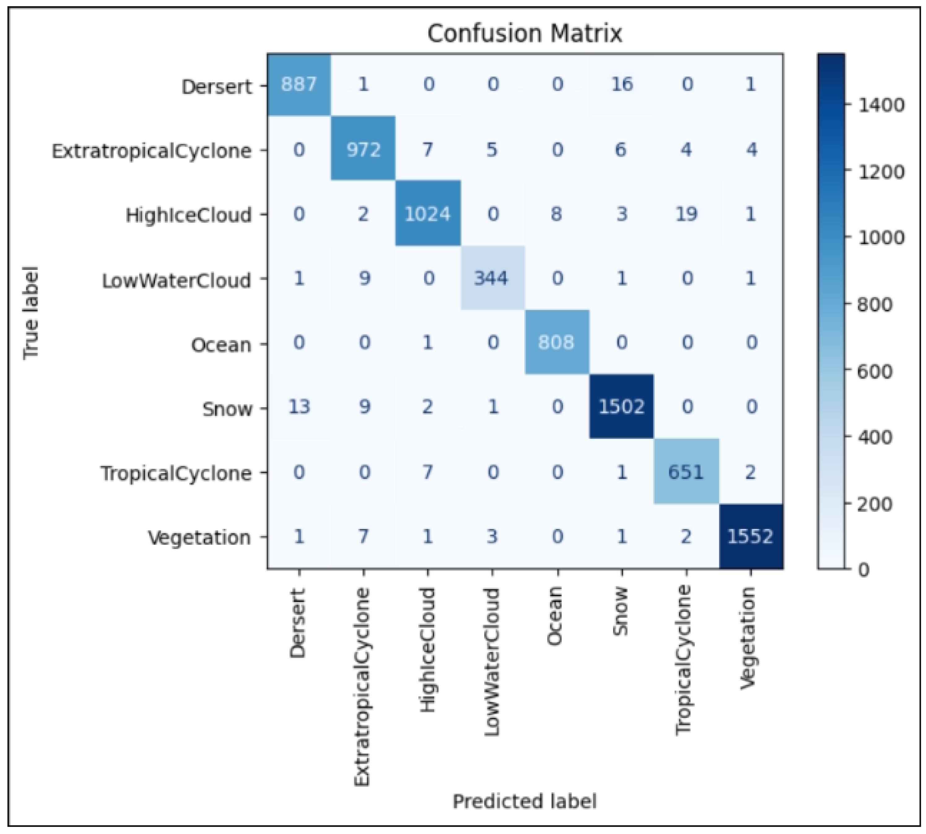
Figure 6.
ROC Curves.
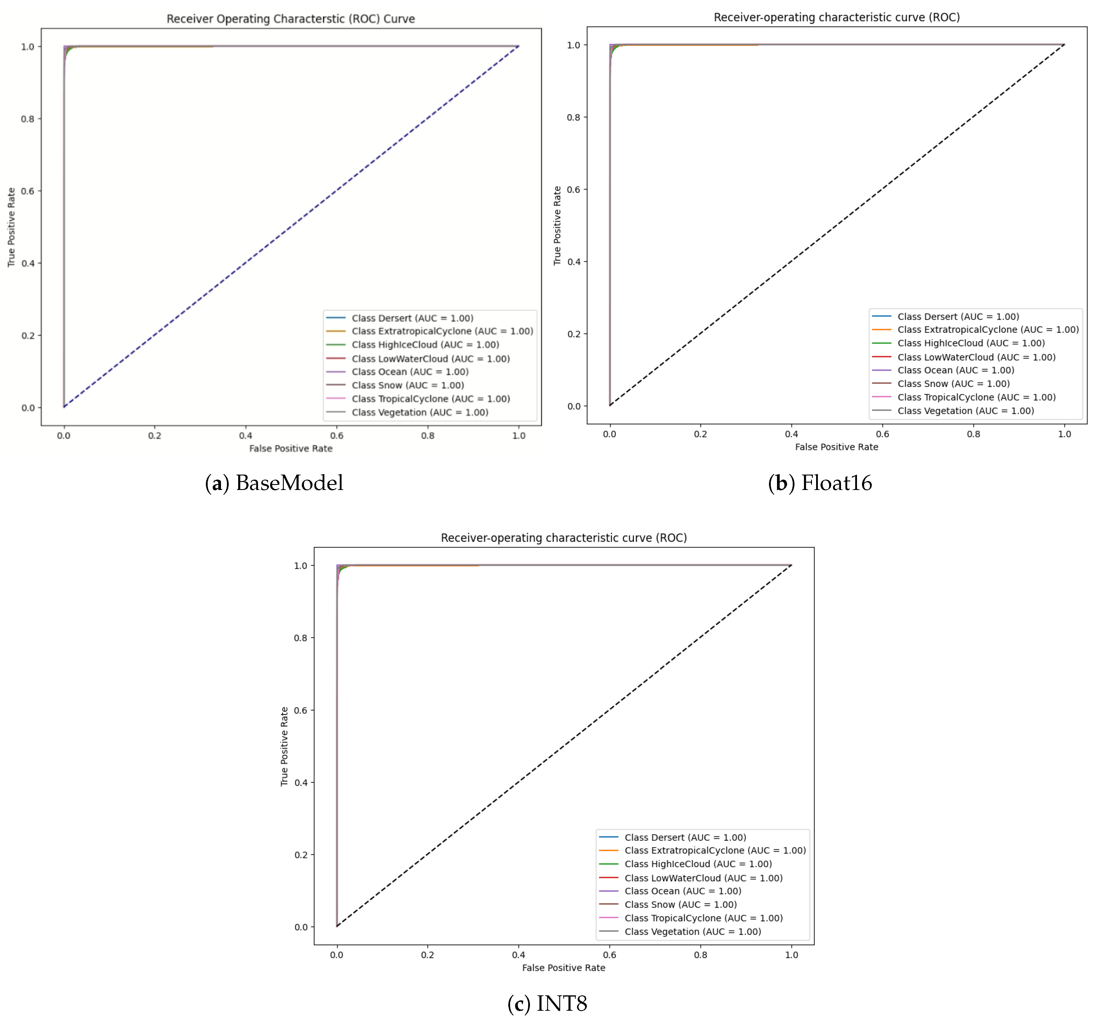
Figure 7.
Precision Recall Curves.
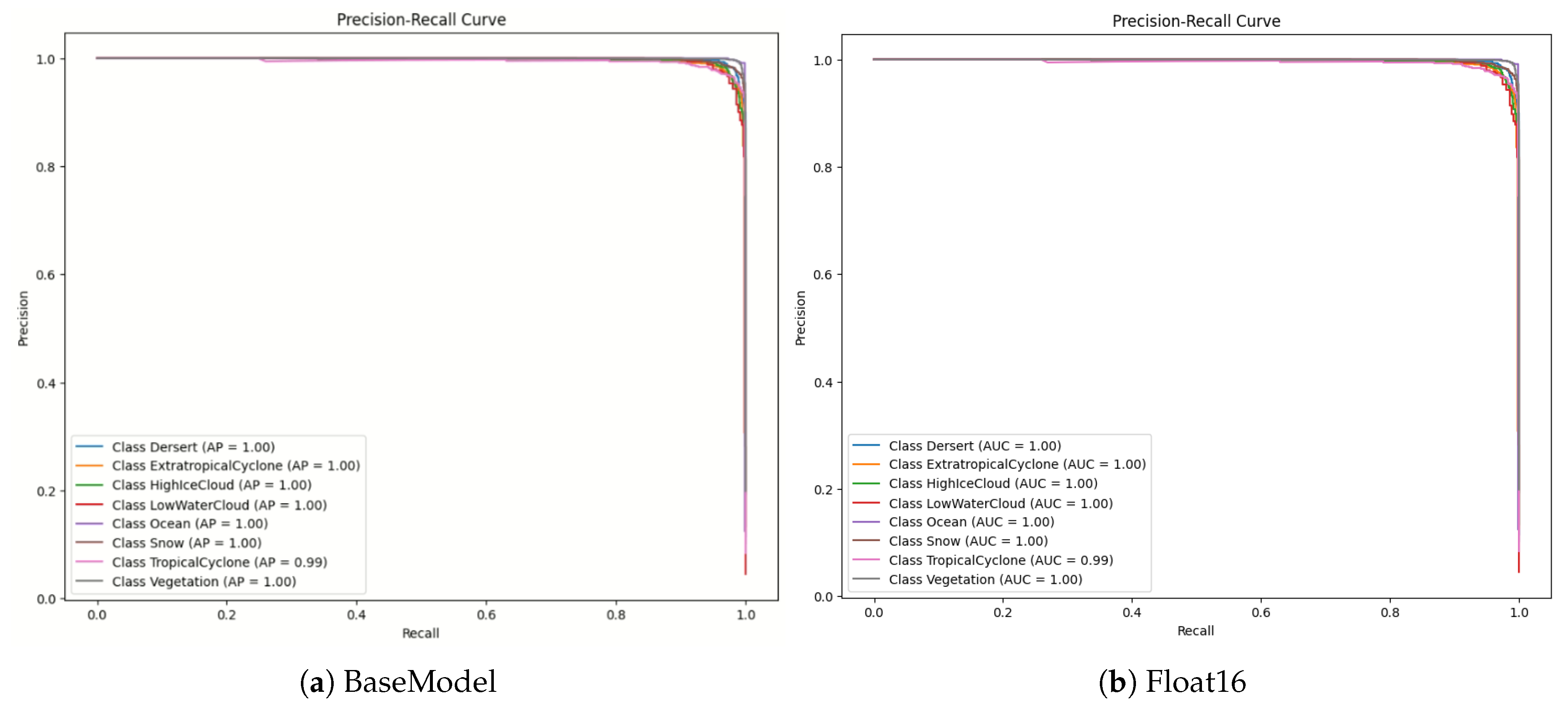
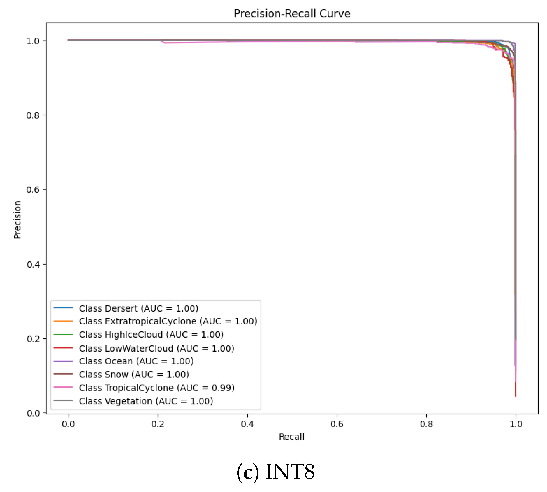
Figure 8.
Performance Curves of SatNet-B3
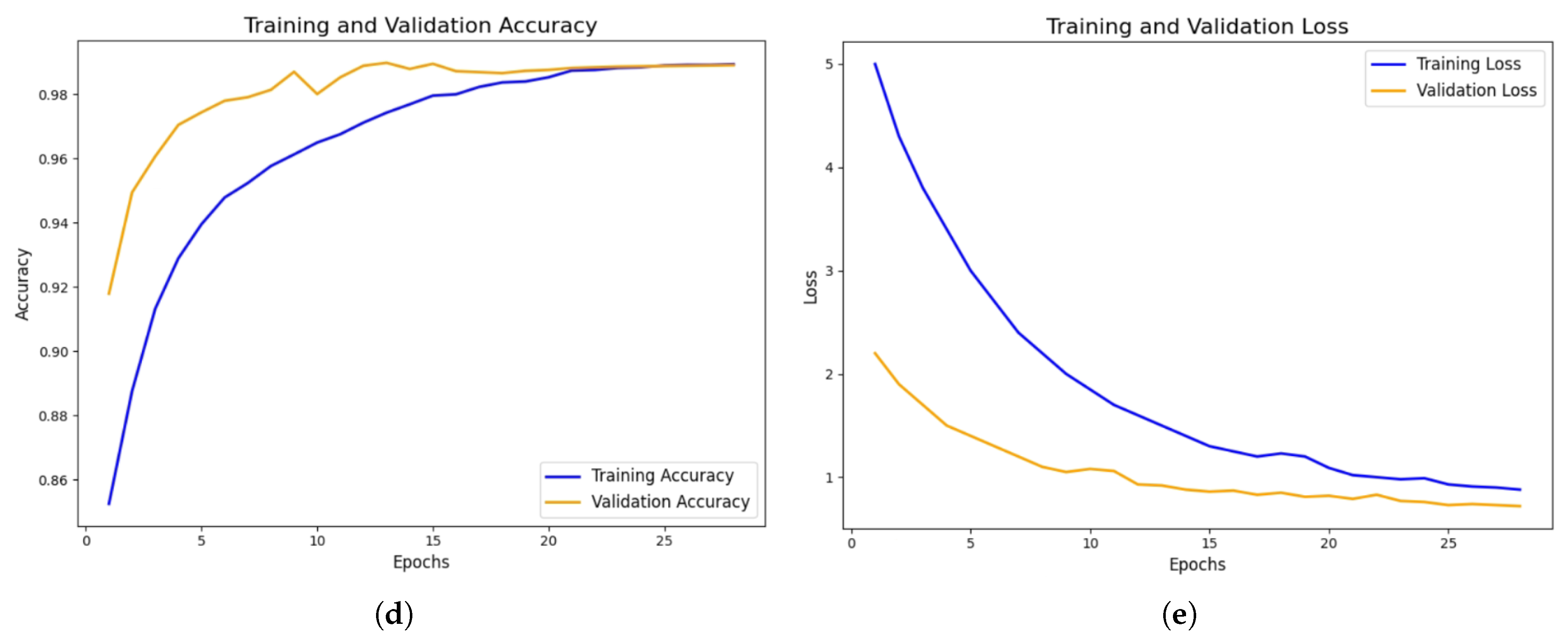
Figure 9.
Interpretability of SatNet B3.
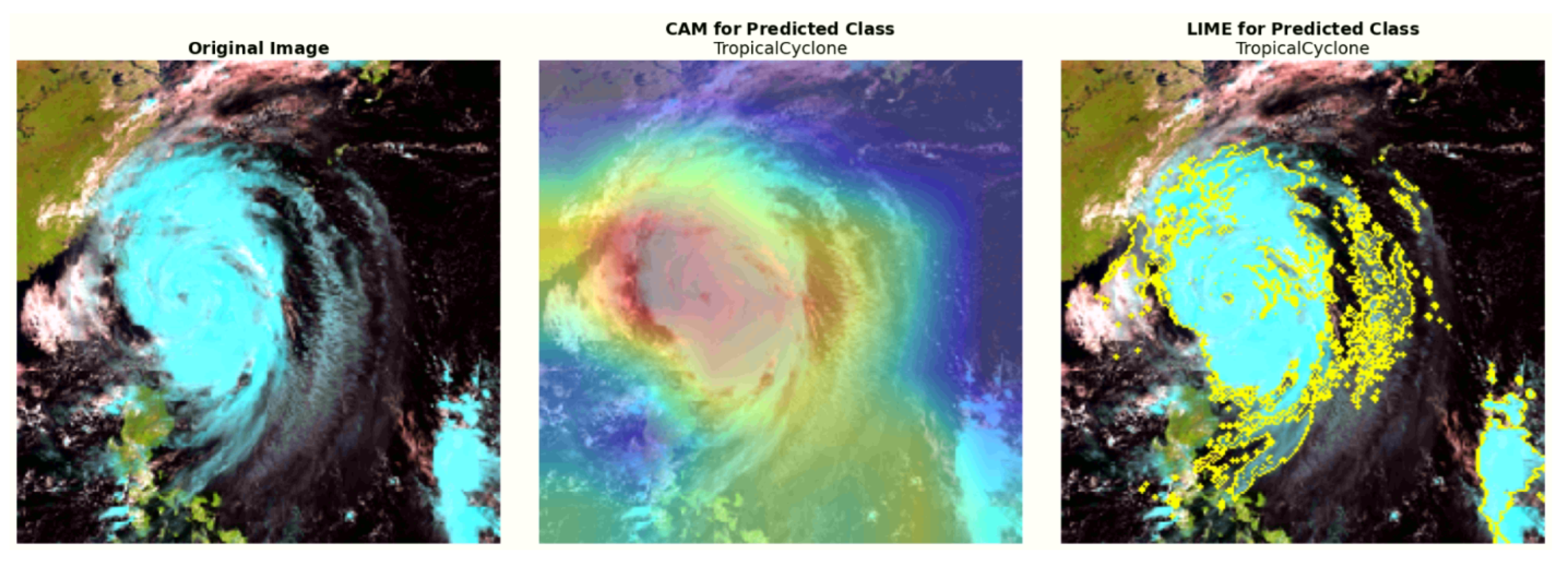
Figure 10.
Images in Different Brightness Conditions.
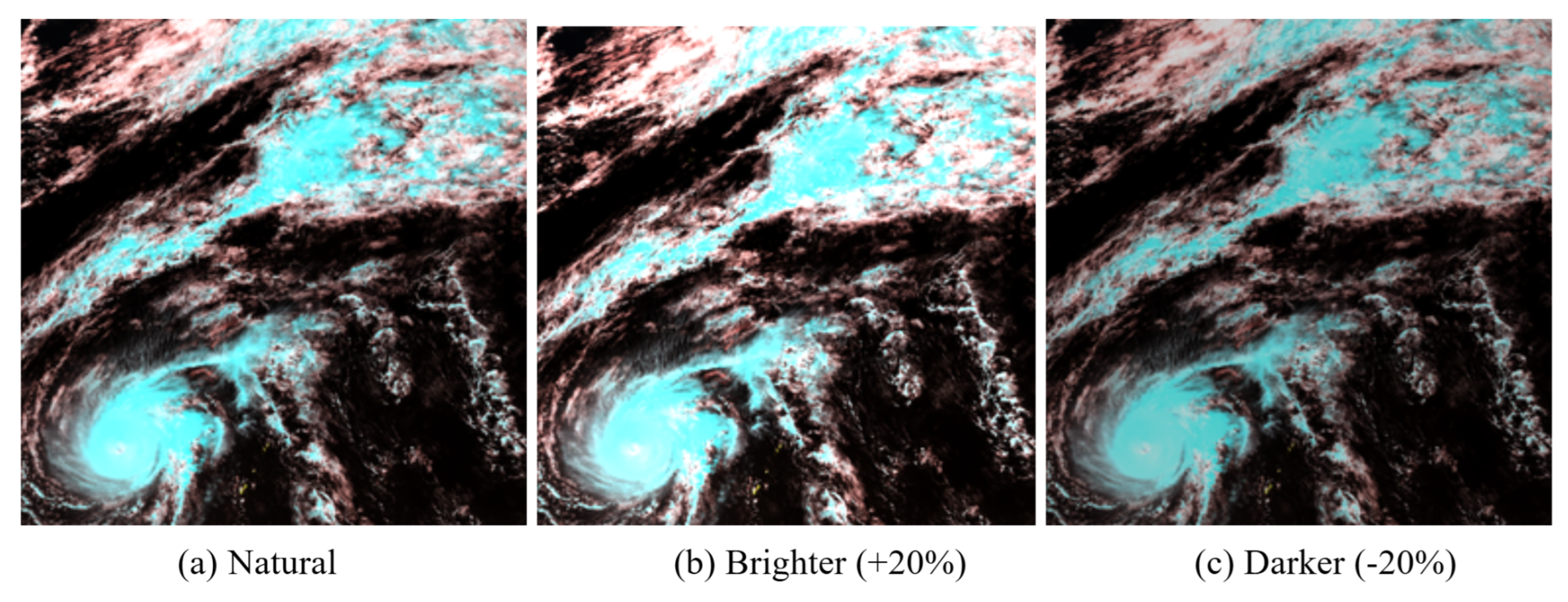
Table 5.
Comparison of quantized models with original.
| Parameter | TensorFlow (H5) | INT8 | Float16 |
|---|---|---|---|
| Accuracy | 98.22% | 98.20% | 98.21% |
| Inference Time | 20.42ms | 103.51ms | 74.66ms |
| File Size | 128.7MB | 11.6MB | 21.3MB |
Table 6.
Experimental Environment for Training Models.
| Environment | Configuration |
|---|---|
| CPU | Intel i7-12700 @2.10 GHz |
| GPU | GeForce RTX 3080 |
| RAM | 32 GB |
| OS | Windows 11 64-bit |
| Python | 3.11 |
Table 10.
Impact of Brightness Variation on Model Performance
| Model | Accuracy (%) | ||
| Natural | Brighter (+20%) | Darker (-20%) | |
| SatNet B3 | 98.22 | 97.73 | 97.92 |
Table 11.
Impact of Blur Variation on Model Performance.
| Model | Accuracy (%) | |||
| Natural | Blur (3×) | Blur (9×) | Blur (13×) | |
| SatNet B3 | 98.22 | 98.02 | 97.86 | 96.90 |
Table 12.
Comparison of existing works on weather classification using satellite imagery
| Ref | Dataset | Approach | Model | Metrics | Implementation |
|---|---|---|---|---|---|
| [8] | CASID | Semantic segmentation | SegNeXt | mIoU= 63.4%, Dice= 76.7% | - |
| [1] | Extreme-Weather | Segmentation | Multichannel Spatiotemporal CNN | mAP= 52.92% | - |
| [3] | Kaggle Cloud Pattern Dataset | Segmentation | U-Net ResNet34 | Dice Coeff= 0.662 | - |
| [4] | INSAT-3DR | Classification | Random Forest | Acc= 90% | - |
| [14] | LSCIDMR | Classification | AlexNet, VGGNet-19, ResNet101, EfficientNet-B5 | Acc= 88.74%, 93.19%, 93.88%, 94.09% | - |
| [2] | LSCIDMR | Classification | SnapResNet152 | Acc= 97.25% | - |
| This Work | Modified LSCIDMR | Classification | SatNet-B3 | Acc= 98% | Raspberry Pi 4 |
Disclaimer/Publisher’s Note: The statements, opinions and data contained in all publications are solely those of the individual author(s) and contributor(s) and not of MDPI and/or the editor(s). MDPI and/or the editor(s) disclaim responsibility for any injury to people or property resulting from any ideas, methods, instructions or products referred to in the content. |
© 2025 by the authors. Licensee MDPI, Basel, Switzerland. This article is an open access article distributed under the terms and conditions of the Creative Commons Attribution (CC BY) license (http://creativecommons.org/licenses/by/4.0/).
Copyright: This open access article is published under a Creative Commons CC BY 4.0 license, which permit the free download, distribution, and reuse, provided that the author and preprint are cited in any reuse.


