
Submitted:
15 May 2025
Posted:
16 May 2025
You are already at the latest version
Abstract
Over the past several centuries, as the global population has experienced a significant increase, there has been a growing need to expand agricultural production and focus on improving the quality of agricultural goods. Contemporary society places emphasis on environmentally friendly practices, sustainable production, and minimally fertilized biological products. With the rapid advancement of machine learning algorithms, precision agriculture has the potential to utilize a wide range of innovative solutions. One such algorithm, YOLOv5 (You Only Look Once), is capable of recognizing objects with high precision in real-time. The identification of wild mushrooms is of significant practical and scientific importance, as certain species are edible and can serve as a viable food source. This research presents a novel architecture utilizing multispectral images and experimental findings from the Yolov5 algorithm on a unique dataset consisting of wild mushroom biomass, including Macrolepiota Procera, with the goal of enhancing the resilience of precision agriculture.
Keywords:
Wild mushroom detection
; Macrolepiota Procera
; Precision Agriculture
; Machine Learning
; Unmanned aerial vehicle
; Multispectral
1. Introduction
The primary production sector has made significant progress in automating and streamlining manufacturing, harvesting, and processing operations in the current industrial era. This has led to improvements in efficiency and reductions in expenses. Furthermore, mushrooms are highly valued for their nutritional properties, including their high levels of vitamins, dietary fibers, and proteins. These properties have been shown to boost the immune system and protect against various forms of cancer [1]. Due to these benefits, there is a growing demand for high-yield, safe harvesting of wild mushrooms. By utilizing wild mushroom cultivation techniques, the primary sector can address the challenges of producing and harvesting agricultural goods in a more sustainable manner [2,3]. Despite the abundance of food available in modern society, the sustainability of food production remains a pressing concern. Factors such as limited arable land, inadequate access to water resources, energy consumption, and the impact of climate change, as well as overpopulation, all contribute to this challenge. In particular, the cultivation of mushrooms requires optimal conditions in terms of temperature and humidity, which can be energy-intensive to maintain. As a result, many mushroom growers resort to collecting wild mushrooms from open fields. However, this process can be complex and time-consuming, as correctly identifying mushrooms in forested areas is challenging. To achieve the desired rate of production [4] and level of quality for end customers, new techniques and methods are introduced to implement creative improvements in agricultural practices and reform conventional operations. The agricultural sector has made significant advancements in automating and enhancing production and processing procedures in the contemporary industrial era. The primary sector has undergone a significant upgrade to new quality standards as a result of the ongoing penetration of high-tech technologies [5], such as Unmanned Aerial Vehicles (UAVs) [6], Robots [7], optimized supply chains, the continuous evolution of Computer Vision (CV) [8], and the continuous improvement of Artificial Intelligence (AI) [9] and Ensemble Learning (EL) [10]. As new approaches are necessary to maintain product quality and sustainability, this problem has grown increasingly widespread in agriculture. Several cutting-edge AI-enabled technologies and specific implementations based on the Machine Learning (ML) [11], Deep Learning (DL) [12], and CV paradigms have impacted the agricultural business in terms of product quality assurance. It is crucial to use these modern technologies to identify mushroom cultivations in natural habitats [13]. This study aims to investigate the difficulty of effectively recognizing wild mushrooms in forest environments using CV, AI solutions and UAVs with RGB and multispectral cameras. An updated dataset of Macrolepiota Procera mushrooms [14,15] and other wild mushroom species is introduced, along with AI-trained and CV identification methods. The updated mushrOom Macrolepiota Procera dEtection dataSet (OMPES) [16] is now named Wild mushrOom dEtection dataSet (WOES) dataset. The difference between the OMPES dataset and WOES is the increase in ground photographs of both Macrolepiota Procera mushrooms and other mushroom species. While there have been significant technological advancements in particular sectors, the adoption of AI methods in agriculture has faced some disadvantages. AI acceptance has decreased, leaving a significant gap in its widespread application. Utilizing ML and DL for mushroom identification improves the product’s quantity, quality, and exploitation of future wild mushroom yields. However, the difficulty of the issue to be solved is inherent. A mushroom may be surrounded by hundreds of weeds or stones of the same hue, significantly increasing the quantity of data that must be processed. Figure 1 depicts various wild mushroom species growing in the forest. Notably, some noteworthy work has been performed on mushroom detection. Regarding mushroom detection and recognition, the authors in [17] aimed to build an object recognition algorithm that could be operated with industrial cameras to detect the development state of edible mushrooms in real-time. This algorithm can be deployed in future autonomous picking equipment. Moreover, in large resolution, small targets (edible mushrooms) have been detected with 98% accuracy. However, with the processing power available today and the rapid expansion of cloud computing, this trade-off of computational power for accuracy is cost-effective. Their study produced significant results in recognizing editable mushrooms. An inevitable drawback of this method is the impact on the aspect ratio and size of the image (see Figure 1).
A significant contribution to the field of mushroom detection and identification was made by [18], in which the authors employed a deep learning-based solution utilizing the attention mechanism Convolution Block Attention Module (CBAM), multi-scale fusion, and an anchor layer. To improve recognition accuracy, the proposed model incorporated hyperparameter evolution during its training. Results indicate that this approach classifies and identifies wild mushrooms more effectively than traditional single-shot detection (SSD), Faster Rcnn, and Yolo series methods. Specifically, the revised Yolov5 model improved the Mean Average Precision (MAP) by 3.7% to 93.2%, accuracy by 1.3%, recall by 1.0%, and model detection time by 2.0%. Notably, the SSD method lagged behind in terms of MAP by 14.3%. Additionally, the model was subsequently simplified and made available on Android mobile devices to enhance its practicality, addressing the issue of mushroom poisoning caused by difficulties in identifying inedible wild mushrooms. In a separate study, [19] compared various machine learning algorithms, including YOLOv5 with ResNet50, YOLOv5, Fast RCNN, and EfficientDet, for the task of discovering chest anomalies in X-ray images. Utilizing VinBigData’s web-based platform, the authors compiled a dataset containing 14 significant radiographic findings and 18,000 images. Through the evaluation of the trained models, it was found that the combination of Yolov5 and Resnet-50 architecture yielded the optimal metric values of Mean Average Precision (MAP) at 0.6 and precision equal to 0.254 and 0.512. Furthermore, this study focuses on the detection of Macrolepiota Procera mushrooms, however, it is acknowledged that the ability to detect other wild mushroom species with a probability factor is crucial for comprehensive wild mushroom detection. By closely examining the characteristics of mushrooms, the specific species can be determined. The ultimate goal of this work is not limited to detecting individual mushrooms in a forest, but also identifying areas with the greatest potential for wild mushroom growth. By having a comprehensive understanding of potential wild mushroom locations, search time and labor can be reduced. Additionally, by observing patterns created by wild mushrooms, the proposed methodology can evaluate these patterns and determine the mushroom species present in a given area with a probability factor. The present study makes three significant contributions to the field of wild mushroom harvesting research. The first contribution is the development of an updated version of the OMPES dataset, now known as the WOES dataset. This dataset is designed for the multivariate identification of wild mushrooms, with a specific focus on the Macrolepiota Procera species. The WOES dataset is highly adaptable, providing researchers with a valuable tool for developing and evaluating strategies for mushroom identification. Continuing, the second contribution is the introduction of a cutting-edge approach for locating wild mushrooms using unmanned aerial vehicles (UAVs) and multispectral cameras. This technique combines real-time UAV surveillance with multispectral photos, enabling the identification of wild mushroom cultivation using the WOES dataset. Lastly, the third contribution of this paper is the proposed architecture for real-time monitoring with low-cost equipment. The machine learning models developed and presented in this work can be applied to images or videos acquired by either UAVs or mobile devices, enabling the detection of wild mushrooms from both ground and aerial imagery. These models can be evaluated in the present study’s evaluation of models, to determine the most reliable model configuration and technique for the dataset.
2. Materials and Methods
2.1. Data Acquisition
The WOES (Wild Mushroom Observation and Exploration System) dataset is a comprehensive collection of examples of wild mushrooms in various stages of development. This dataset aims to facilitate the training of machine learning and deep learning techniques for the identification and classification of wild mushroom species. A Data Acquisition System (DAQ) is employed as the primary means of data collection. The DAQ captures environmental signals and converts them into machine-readable data, while software is used to process and store the acquired data. It is crucial to collect data during a specific time window, with the optimal period for the majority of mushroom species being September and October. During this time, meteorological assessments of the search area should be conducted periodically. Additionally, it is important to note that environmental factors such as temperature and relative humidity play a crucial role in the development of wild mushrooms. Ideal conditions for mushroom growth are typically formed when high temperatures are preceded by heavy precipitation in the same region. This is because mushrooms require a warm, humid habitat for optimal growth. It is noteworthy that the geographic place of data collection in the OMPES and WOES datasets is in Western Macedonia, Greece. The spot of the study has a latitude of "40.155903863645534" and a longitude of "21.434814591442194"—these coordinates were provided by Google Maps, which utilizes the World Geodetic System (WGS) 84 format. The Keyhole Markup Language (KML) file presents the research area in Figure 2.
In the context of this work, we utilized a multi-copter drone equipped with an RGB and multispectral camera. Figure 3 demonstrates the creation and assembly of a customized multi-copter UAV using low-cost materials. The main objective is to gather photographs and videos of the defined region and analyze them to be embedded in the WOES dataset. The secondary goal is to participate in a scenario that involves detecting wild mushroom cultivations in a large forest.
The essential components of the drone are the OpenPilot CC3D Revolution (Revo) flight controller, four BR2205 2300KV motors, a BN-880 GPS Module U8 with a Flash HMC5883 compass, MPL3115A2 - I2C Barometric Pressure/Altitude/Temperature sensor board, a WiFi antenna 2.4GHz 5dBi 190mm, parrot sequoia+, and the Tattu FunFly 1800mAh 14.8V Lipo battery pack. Moreover, the flight controller is configured using Cleanflight, an open-source program that supports a range of current flight boards. In addition, the 2.4 GHz FlySky FS-i6 is used to transmit the control signal. We utilize a Raspberry Pi Zero 2 with an RPi camera board version 2 that supports 8 MP image resolution and FHD quality for video as the central processing unit for streaming to the base station. It is worth noting that the primary function of the U.FL connector is to mount external antennas on boards. Furthermore, the raspberry pi zero two does not have a U.FL connector on its board. Its installation on the board must be done manually and cannot be purchased from the market. In this work, the proposed solution employs a field-based base station in proximity to the drone’s operational area. The base station utilized in this study is a laptop computer that communicates with the Raspberry Pi on the drone via WiFi. It is well-known within the research community that WiFi technology offers a high packet transmission rate, but has a limited communication range. To mitigate this limitation, the drone is equipped with a live footage broadcasting capability which can be enhanced through the deployment of external antennas on both the drone and base station. Specifically, an Alfa AWUS036ACH external antenna is utilized on the base station to extend the WiFi range.
2.2. Data Preparation
This study presents the methodology employed in the preparation of data for the training of machine learning models with high accuracy. The data consists of images of mushrooms that have been annotated with their corresponding classes. Two trained machine learning models have been developed, one for the recognition of mushroom entities and the other for the identification of a characteristic unique to Macrolepiota procera. The latter model is particularly designed to differentiate between Macrolepiota procera and Agaricus Campestris species prevalent in the Grevena region. The annotation process was carried out using an internet platform (accessed on Nov. 18, 2022, https://www.makesense.ai/) and the labels were exported as Yolov5-formatted text files. The data were then segregated into training and validation sets and batches. The training data was utilized to feed the model, while the validation set, comprising unrevealed data, was used for the self-evaluation of the trained model. The distribution of labels in the OMPES and WOES datasets is depicted in Figure 4. The files comprise a single class and include aerial and ground images. The OMPES dataset has 535 photos, while WOES has 907. It is worth noting that two machine learning models will be trained from the WOES dataset, of which the first utilizes all the photos in the dataset while the second uses only 44.55% (404 photos). The first WOES model is referred to as "Wild mushrooms" and the second one, which detects one of the main characteristics of the mushrooms, Macrolepiota procera, will be referred to as the "Macrolepiota procera characteristic". The reduced abundance of the "Macrolepiota procera characteristic" model is due to the fact that the dataset does not include only mushrooms of Macrolepiota procera. In addition, the number of labels used to train the AI models is depicted in the upper-left corner of Figure 4. The lower-left corner of Figure 4 (b) serves as the origin for the normalized target location map, which is generated using a right-angle coordinate system. The relative values of the horizontal and vertical coordinates x and y are used to determine the relative locations of the targets. Furthermore, the target size distribution is relatively concentrated, as seen by the normalized target size map in Figure 4 (c). The proposed methodology’s most innovative part is aerial multispectral imagery. Using the Parrot Sequoia+ camera, multispectral pictures are obtained. This camera has five spectral bands: RED, REDEDGE, GREEN, Near-InfraRed (NIR) and RGB. The wavelength of each spectrum except RGB is 660nm (RED), 735nm (REDEDGE), 550nm (GREEN), and 790nm (NIR). These spectra are depicted in Figure 5, which shows a part of the study area. Each Region of Interest (ROI) consists of four corners corresponding to the image’s cartesian coordinates. For instance, if the height and width of an image are 100 pixels (100 X 100), the ROI may contain 25 pixels for height and 40 pixels for width (25 X 40). It may have a lower left corner at (10, 10), an upper left corner at (35, 10), a lower right corner at (10, 50), and an upper right corner at (35, 50).
Notably, the RED, REDEDGE, GREEN, and NIR spectra have pixel sizes of 1200 by 960. Figure 6 illustrates a typical difference between the RED and NIR bands. In this scenario, a ROI of 140 pixels in height and 200 pixels in width (140 X 200) was selected, in which the red line is tangent to the mushroom in the NIR spectrum and the green line is tangent to the mushroom in the RED spectrum, respectively. Therefore, the difference between the two bands is noticeable along the horizontal axis. Variations on the vertical and horizontal axes are also found in the remaining spectra. Therefore, it is imperative to modify all the spectra, as their proper processing will require a one-to-one matching of all the spectra.
Consequently, all multispectral images must be suitably adjusted. The bands must initially be adjusted into the desired band. In this work, the RED, GREEN, RGB, and NIR bands were adjusted in reference to the REDEDGE band. Python libraries for computer vision were used throughout the transformation procedure. The most important libraries are PIL, NumPy, and OpenCV (Open Computer Vision). Before developing the script, the proper parameters must be determined. Geographic Information System (GIS) applications may be used to locate these variables. Essentially, the RED, NIR, REDEGE, and GREEN bands are rotated to the right by ninety degrees, while the RGB spectrum is rotated to the left by ninety degrees. Furthermore, the dimensions of the RGB band image should be changed from 3456 X 4608 to 960 X 1280. Table 1 depicts the transformations for each spectrum concerning the REDEDGE band. The final step is to crop all multispectral images to 925 X 1165 pixels. Notably, a deviation of two pixels was observed when the above method was used on a hundred multispectral images. Conclusively, the imagery conversion process is described as challenging yet vital for their utilization.
As previously stated, the drone utilized in this study was equipped with a multispectral camera. The multispectral camera captures data based on the reflection frequencies of objects when taking photos. Furthermore, at a low altitude of 3 to 15 meters above the ground, several bands in multispectral images reveal the presence of wild mushrooms. The frequency range of mushrooms can be determined using GIS applications. In this project, the GIS tool employed was QGIS, a free software. This manual process applies to all species and regions of wild mushrooms. Table 2 depicts the optimal frequencies in multispectral images for identifying wild mushrooms. Additionally, Figure 7 illustrates the application of the thresholds from Table 2 to the multispectral images of each spectrum.
2.3. The Main Methodology
In this work, an architecture will be followed, which includes a drone, a base station, and a drone operator. WiFi Direct is used for communication between the drone and the base station, while a 2.4 GHz transmitter handles the drone’s telemetry. The architecture is depicted in Figure 8.
2.4. Phase One
In the first phase, the pilot operates the drone at a high altitude of 40 to 100 meters over an area devoid of thick tree cover. The pilot establishes a connection with the multispectral camera Parrot Sequoia+. The base station connects to the camera’s hotspot, allowing it to access its IP address. Correspondingly, the operator establishes a connection between the Raspberry Pi and the multispectral camera. The raspberry pi transmits live video with the RPi camera board to the base station through the camera hotspot. The transmission is done with the libcamera library. In more detail, the libcamera library is a new software library designed to provide direct support for complicated camera systems from the Linux operating system. Furthermore, the operator establishes a wireless connection between the Parrot Sequoia+ camera and the base station before executing the command to capture a multispectral image. Capturing a multispectral image takes approximately five seconds, making it crucial for the drone to maintain a constant posture throughout this period. The camera archives the picture locally. After the completion of picture capture, five stages are conducted:
- Processing the band images to adjust them to the selected spectrum (REDEDGE).
- Calculating the Normalized Difference Red Edge Index (NDRE) vegetation index.
- Identifying potential locations with wild mushrooms.
- Calculating the probability of finding wild mushrooms in each location.
- Sending the processed RGB spectrum with the locations and probability of the wild mushrooms to a PNG image file via WiFi to the base station.
In Subsection 2.2, the fitting, preparation, and general processing of the bands were addressed in depth. Vegetation Indices (VIs) derived from remote sensing-based canopies are simple and practical methods for quantitative and qualitative assessments of vegetation cover, vigour, and growth dynamics, among other uses. These indices have been extensively utilized in remote-sensing applications via various satellites, and UAVs [20]. NDRE measures the chlorophyll content in plants. The optimal period to apply NDRE is between the middle and end of the growing season when plants are fully developed and ready to be harvested. At this time, it would be less beneficial to employ alternative indexes. NDRE is a remote-sensing vegetation indicator that measures the chlorophyll content of plants [21]. The NDRE equation is:
The Normalized Difference Vegetation (NDVI) evaluates the greenness and density of vegetation in satellite and UAV imagery in the simplest terms possible. The healthy plants’ spectral reflectance curve determines the difference between the visible RED and NIR bands. This difference is represented numerically by the NDVI, which ranges from -1 to 1. Consistently calculating the NDVI of a crop or plant over time may disclose a great deal about environmental changes. In other words, the NDVI may be used to evaluate plant health remotely [22]. The NDVI equation is:
The Optimization of Soil Adjusted Vegetation Index (OSAVI) vegetation index considers reflectance in the NIR and RED bands. The fundamental difference between the two indices is that OSAVI considers the traditional value of the canopy backdrop adjustment factor (0.16) [23]. The OSAVI equation is:
This research used vegetation indices to detect locations yielding wild mushrooms. Considered vegetation indicators included NDVI, OSAVI, and NDRE. Figure 9 illustrates the vegetation indices that were generated using the QGIS application. It is essential to understand that the QGIS software exports the vegetation indices as Tif files to be utilized in other applications. Moreover, Figure 9 reveals that the NDRE vegetation index has a more satisfactory result than NDVI and OSAVI because there are areas with elevated value changes compared to the overall image.
Computer vision is used only for locating mushroom patches within the NDRE vegetation index. Initially, the script utilizes the NDRE and the PIL library to analyze the Tif file. Then, a new image is constructed with a white background. This is followed by two FOR loops that access every pixel in the imported image. Those pixels with a value higher than or equal to 0.7 are then colored red (255, 0, 0); otherwise, they are colored black (0, 0, 0); the resulting image is depicted in Figure 10 (a). This image will be referred to as HighValueSpots and be a PIL image object.
The HighValueSpots image is then blurred using the cv.filter2D function with arguments a) the image, b) -1, and c) a kernel. The initial value of the first parameter is the HighValueSpots image, while the required depth of the target image is specified by parameter -1. The number -1 indicates that the resultant image’s depth will be the same as the source image’s. The kernel is a short, two-dimensional table holding values that indicate how much of the surrounding pixel values should be used to determine the intensity value of the current pixel. Kernels are typically odd-length square arrays, such as 3 X 3, 5 X 5, and 7 X 7. The 80 X 80 matrix recommended for this study is constructed with the function np.ones((80,80),np.float32)/25. Choosing large values, such as 80, is primarily motivated by the need to prevent minor gaps between the groups. Figure 10 (b) displays the result, the BlurredHighValueSpots image, and a PIL image object with the name BlurredHighValueSpots. Furthermore, the K-means algorithm divides the BlurredHighValueSpots image into two color groups, the background and the red color. K-means clustering is initially a method for categorizing data points or vectors based on their proximity to their respective mean points. This leads to dividing the data points or vectors into cells. When applied to an image, the K-means clustering algorithm considers each pixel as a vector point and generates k-clusters of pixels [24]. The K-means algorithm is directly called using the function cv.kmeans, which requires five parameters:
- Samples: The data type should be np.float32, and each feature should be placed in a separate column.
- Nclusters (K): Number of clusters required.
- Criteria: It is the condition for terminating an iteration. When these conditions are met, the algorithm stops iterating.
- Attempts: Specifies the number of times the algorithm is conducted with different beginning labellings. The method returns the labels that result in the highest degree of compactness. This density is returned as the output.
- Flags: This flag specifies how initial centres are obtained.
Therefore, the cv.kmeans function is executed with the following parameters: a) np.float32(), b) 2, c) cv.TERM_CRITERIA_EPS + cv.TERM_CRITERIA_MAX_ITER, d) 10, and e) cv.KMEANS_RANDOM_CENTERS. The cv.TERM_CRITERIA_EPS criterion refers to stopping the algorithm iteration when a given level of accuracy is achieved, while the cv.TERM_CRITERIA_MAX_ITER criterion refers to stopping the algorithm after the specified number of iterations. Figure 10 (c) displays the result, the modified BlurredHighValueSpots image, as a PIL image object named GroupedBlurredHighValueSpots. Using the cv.findContours and drawContours functions, each red region of the GroupedBlurredHighValueSpots image is accessible. Initially, explanations for contours may be as simple as a line connecting all continuous points (along the border) with the same color or intensity. Contours are a valuable tool for form analysis and item identification and detection. The cv.findContours function locates the red regions in the GroupedBlurredHighValueSpots picture using three parameters: a) cv2.Canny(image, 140, 210); b) cv2.RETR LIST; and c) cv2.CHAIN APPROX NONE. The image parameter accepts the image GroupBlurredHighValueSpots as its value. In addition, the cv2.RETR LIST argument returns all contours without establishing any parent-child connection. Under this concept, parents and children are equal and serve as a guideline—lastly, the cv2.CHAIN APPROX NONE argument eliminates all unnecessary points and compresses the contour. The drawContours function is responsible for drawing contours on an image. This function has as parameters: a) the image to draw the contours on; b) the contours in tabular form; c) the color of the contour line; and d) the thickness of the line. The program has been given as follows: a) image; b) contours; c) (0, 255, 0); and d) 5. Figure 10 (d) portrays the outcome, the modified GroupBlurredHighValueSpots image, as a PIL image object documented as ContourGroupedBlurredHighValueSpots. The last stage is calculating the probability of finding wild mushrooms in each area. A formula that calculates this probability will need to be created to attain this purpose. Initially, two successive FOR iterations will access all pixels of each contour in the TIF image file of the NDRE vegetation index. Simultaneously, each contour’s average of the NDRE values (avg) and the maximum NDRE value (max) will be determined. At the completion of the entire access to all pixels in each area, the probability of finding mushrooms is computed using the following formula:
Notably, the probability and contours are rendered in the RGB spectrum, as shown in Figure 10 (e), and the picture (MushroomLocations) is sent to the base station using the socket library.
2.5. Phase Two
After evaluating the MushroomLocations image with the potential locations Figure 10 (e), the drone operator subsequently flies the drone at a lower altitude to the targeted areas to verify the presence of wild mushrooms, as seen in Figure 8 (b). It is important to note that the drone includes an altimeter sensor, which helps measure the drone’s altitude. In real-time, the drone sends its location (longitude and latitude) and altitude (meters) relative to the ground to the base station. This allows the base station to execute machine-learning models for mushroom identification through the live broadcast outlined in subsection Phase one. In this study, the Yolov5 algorithm is applied for object identification, capable of live stream recognition. The following command provides a sample example: python detect.py –source url_stream. The base station begins detecting wild mushrooms in the live stream as soon as the drone descends below 20 meters in altitude. In addition, if the drone operator is uncertain about the existence of wild mushrooms, he may take a picture with the multispectral camera to determine whether or not mushrooms are present. Subsection Data Preparation provides a comprehensive examination of multispectral image processing. As illustrated in Figure 7 (c), the RED band outperforms the other bands. After acquiring and processing the multispectral image, the raspberry pi onboard the drone transmits the processed RED band image to the Base Station over WiFi. Two Yolov5 ML models are applied at the base station for mushroom detection. The first model identifies wild mushroom specimens, while the second recognizes a feature of Macrolepiota procera mushrooms. The algorithm generates an ROI containing the recognized objects for each spotted mushroom. The system then performs a second detection at each ROI to identify wild mushroom species. If it identifies an object inside the ROI, the wild mushroom is a member of the Macrolepiota Procera species. Alternately, it may be Agaricus Campestris if it does not distinguish any objects inside the ROI. Figure 11 depicts the pipeline of phase two.
Additionally, after running the first model for the broader search for wild mushrooms, the ROIs are saved as jpg files. These images can be saved by adding the –crop-img flag to the detection command. OnlyWildMushrooms refers to the images subjected to machine vision processing to effectively highlight the characteristics of Macrolepiota procera mushrooms. The script adjusts the brightness and contrast of the mushroom images in order to highlight the dark mottling in the centres of the mushrooms. The libraries OpenCV, NumPy, and PIL are used for image processing. The function ImageEnhance.Brightness(image).enhance(factor) modifies the image’s brightness, while the ImageEnhance.Contrast(image).enhance(factor) modifies the image’s contrast. Image and factor are the two parameters for each of these functions. The Image argument initially contains the OnlyWildMushrooms images, while the factor parameter is a floating point number that controls the augmentation. Furthermore, the value 1.0 always returns a duplicate of the original image; lower numbers indicate less color (brightness, contrast, etc.), while higher values indicate more. This value is not restricted in any way. In this study, the factor value for adjusting brightness is 0.1, while the factor parameter for adjusting contrast is 10. These images will be named ProcessedOnlyWildMushrooms and saved in jpg files. The second model will then be executed to detect the distinctive feature of the wild mushroom Macrolepiota Procera in the photos of ProcessedOnlyWildMushrooms. Figure 11 depicts the proposed pipeline’s outcome and operational procedures.
3. Results
In this study, a mid-to-high-end testbed was utilized for training the detection model. Specifically, a Linux workstation running Ubuntu 20.04, equipped with an Intel Core i7 processor, 64 GB of RAM, and an NVIDIA RTX 3080 GPU with 10 GB of GPU memory was employed. Two machine learning models, "Wild Mushrooms" and "Characteristic Procera," were trained using the Yolov5 library. Figure 4 illustrates the features of the data used for training the models. It is worth noting that the models were trained utilizing the pre-trained Yolov5 model provided by the Yolov5 library. Furthermore, it was determined that the default settings for training the models required improvement. To address this, the evolving program provided by the Yolov5 library was employed to determine the optimal parameters for training the models. The evolving program implements a Genetic Algorithm (GA), a metaheuristic inspired by natural selection, which is part of the broader class of Evolutionary Algorithms (EA). Genetic algorithms are commonly used to develop high-quality solutions for optimization and search problems. It is important to note that machine learning hyperparameters can affect various training elements, and determining their optimal values can be challenging. Traditional methods such as grid searches may become infeasible due to a) the high dimensionality of the search space, b) the unknown correlations between the dimensions, and c) the costly nature of evaluating the fitness at each point, making GA a suitable candidate for hyperparameter searches. In this study, both models were evolved for 1000 iterations. The creators of Yolov5 recommend a minimum of 300 iterations. Table 3 presents the default settings and those produced by the evolving script. The first five hyperparameters are considered the most important and frequently modified parameters. Specifically, the "lr0" hyperparameter represents the initial learning rate of the training process, while the "lrf" hyperparameter represents the final learning rate. Momentum is a measure of the magnitude of the algorithm’s step at each iteration of the learning process. It is important to note that momentum should be kept moderate in complex scenarios to preserve the learning trajectory of the problem. The "weight decay" hyperparameter is used as an additional form of regularization. The "warmup epochs" and "warmup momentum" hyperparameters are employed in conjunction with a slow learning rate to achieve a low percentage of errors at the beginning of the training process. Additionally, all models were trained for 1200 epochs and a batch size of 8.
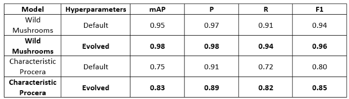
Continuing, in the context of this research a total of four models were trained, including two with default hyperparameters and Evolve script parameters. The outcomes of the training are shown in Table 4. Four qualitative metrics were employed to evaluate the trained models and select the optimal trained network. These metrics include: a) Precision, b) Mean Average Precision (mAP), c) Recall, and d) F1 score. Precision is the ability to correctly identify and classify objects in an image. The only difference between all ground truths is a small variance in recall vs precision. The Average Precision (AP) of each class is calculated separately and the results are combined.
These AP scores are added together to form the measure mAP, and thus the mean AP score across all classes. The F1 score may be seen as the harmonic mean of accuracy and recall, with the highest score being one and the worst score being zero. Precision and recall contribute the same proportion to the F1 score. Equation 5 depicts the F1 scoring formula. Several hyperparameters must be modified for CNN to classify objects inside images accurately. Notably, the enhanced script developed in the context of this research was applied to the Wild Mushrooms model and demonstrated a 2% improvement over the original model, while the Characteristic Procera model showed a 5% improvement. Despite the tiny percentages, the improvement is considerable.
The confusion matrix is a commonly used table to evaluate the performance of a classification model trained with an unknown dataset by an artificial intelligence model, when the actual values are known. Additionally, the columns of the confusion matrix represent the predicted class, while the rows represent the actual class. The sum of each column is equal to one, and the value in each row represents the percentage of predictions in the corresponding category. Furthermore, True Positives (TP) are instances in which the model accurately predicted that the ground-truth item belongs to the class. True Negatives (TN) indicate that the model correctly predicts that the item is not a member of the class. False Positives (FP) occur when the model incorrectly predicts that an item does not belong to a particular class when it does. False Negatives (FN) occur when the model incorrectly predicts that an item does not belong to a class when it does. In conclusion, the majority of objects were accurately predicted, indicating that the models performed well. Figure 12 shows the confusion matrix graphs for the two models.
4. Conclusions
In conclusion, this research has highlighted the need for a comprehensive approach to address the growing challenges facing the agricultural industry. The use of DL-oriented solutions has become an essential foundation for ensuring product quality in modern applications in the primary sector, particularly in precision agriculture. The experimental findings of this research have demonstrated that it is possible to locate wild mushroom yields and identify the species Macrolepiota procera with an accuracy of over 90%. Furthermore, the process of identifying wild mushrooms took only 30 minutes to complete. The research opens up many exciting possibilities for future research, including the potential to extend the WOES dataset to include other mushroom species and their unique characteristics. Additionally, the WOES dataset can be adapted for use on mobile devices and even UAVs, and with the use of cloud services, the process can be automated without the need for personnel in the field. This research is an important step forward in the development of precision agriculture and serves as a powerful reminder of the potential of DL-oriented solutions to revolutionise the agricultural industry.
Acknowledgments
This research was co-funded by the European Regional Development Fund of the European Union and Greek national funds through the Operational Program Western Macedonia 2014-2020, under the call “Collaborative and networking actions between research institutions, educational institutions and companies in priority areas of the strategic smart specialization plan of the region”, project ”Smart Mushroom fARming with internet of Things - SMART”, project code: DMR-0016521.
References
- Park, H. J. (2022). Current uses of mushrooms in cancer treatment and their anticancer mechanisms. International Journal of Molecular Sciences, 23(18), 10502. [CrossRef]
- Garibay-Orijel, R., Córdova, J., Cifuentes, J., Valenzuela, R., Estrada-Torres, A., & Kong, A. (2009). Integrating wild mushrooms use into a model of sustainable management for indigenous community forests. Forest Ecology and Management, 258(2), 122–131. [CrossRef]
- Agrahar-Murugkar, D., & Subbulakshmi, G. (2005). Nutritional value of edible wild mushrooms collected from the Khasi hills of Meghalaya. Food Chemistry, 89(4), 599–603. [CrossRef]
- Rózsa, S., Andreica, I., Poșta, G., & Gocan, T. M. (2022). Sustainability of Agaricus blazei Murrill mushrooms in classical and semi-mechanized growing system, through economic efficiency, using different culture substrates. Sustainability, 14(10), 6166. [CrossRef]
- Moysiadis, V., Sarigiannidis, P., Vitsas, V., & Khelifi, A. (2021). Smart farming in Europe. Computer Science Review, 39, 100345. [CrossRef]
- Boursianis, A. D., et al. (2022). Internet of Things (IoT) and agricultural unmanned aerial vehicles (UAVs) in smart farming: A comprehensive review. Internet of Things, 18, 100187. [CrossRef]
- Amatya, S., Karkee, M., Zhang, Q., & Whiting, M. D. (2017). Automated detection of branch shaking locations for robotic cherry harvesting using machine vision. Robotics, 6(4), 31. [CrossRef]
- Uryasheva, A., et al. (2022). Computer vision-based platform for apple leaves segmentation in field conditions to support digital phenotyping. Computers and Electronics in Agriculture, 201, 107269. [CrossRef]
- Zahan, N., Hasan, M. Z., Malek, M. A., & Reya, S. S. (2021). A deep learning-based approach for edible, inedible and poisonous mushroom classification. Proceedings of ICICT4SD, 440–444. [CrossRef]
- Picek, L., et al. (2022). Automatic fungi recognition: Deep learning meets mycology. Sensors, 22(2), 633. [CrossRef]
- Lee, J. J., Aime, M. C., Rajwa, B., & Bae, E. (2022). Machine learning-based classification of mushrooms using a smartphone application. Applied Sciences, 12(22), 11685. [CrossRef]
- Siniosoglou, I., Argyriou, V., Bibi, S., Lagkas, T., & Sarigiannidis, P. (2021). Unsupervised ethical equity evaluation of adversarial federated networks. ACM International Conference Proceedings. [CrossRef]
- Martínez-Ibarra, E., Gómez-Martín, M. B., & Armesto-López, X. A. (2019). Climatic and socioeconomic aspects of mushrooms: The case of Spain. Sustainability, 11(4), 1030. [CrossRef]
- Barea-Sepúlveda, M., et al. (2022). Toxic elements and trace elements in Macrolepiota procera mushrooms from southern Spain and northern Morocco. Journal of Food Composition and Analysis, 108, 104419. [CrossRef]
- Adamska, I., & Tokarczyk, G. (2022). Possibilities of using Macrolepiota procera in the production of prohealth food and in medicine. International Journal of Food Science, 2022. [CrossRef]
- Chaschatzis, C., Karaiskou, C., Goudos, S. K., Psannis, K. E., & Sarigiannidis, P. (2022). Detection of Macrolepiota procera mushrooms using machine learning. IEEE WSCE, 74–78. [CrossRef]
- Wei, B., et al. (2022). Recursive-YOLOv5 network for edible mushroom detection in scenes with vertical stick placement. IEEE Access, 10, 40093–40108. [CrossRef]
- Zhang, D., et al. (2022). Research and application of wild mushrooms classification based on multi-scale features to realize hyperparameter evolution. Journal of Graphics, 43(4), 580. [CrossRef]
- Luo, Y., Zhang, Y., Sun, X., Dai, H., & Chen, X. (2021). Intelligent solutions in chest abnormality detection based on YOLOv5 and ResNet50. Journal of Healthcare Engineering, 2021. [CrossRef]
- Xue, J., & Su, B. (2017). Significant remote sensing vegetation indices: A review of developments and applications. Journal of Sensors, 2017. [CrossRef]
- Davidson, C., Jaganathan, V., Sivakumar, A. N., Czarnecki, J. M. P., & Chowdhary, G. (2022). NDVI/NDRE prediction from standard RGB aerial imagery using deep learning. Computers and Electronics in Agriculture, 203, 107396. [CrossRef]
- Solano-Alvarez, N., et al. (2022). Comparative analysis of the NDVI and NGBVI as indicators of the protective effect of beneficial bacteria in conditions of biotic stress. Plants, 11(7), 932. [CrossRef]
- Steven, M. D. (1998). The sensitivity of the OSAVI vegetation index to observational parameters. Remote Sensing of Environment, 63(1), 49–60. [CrossRef]
- Kılıç, D. K., & Nielsen, P. (2022). Comparative analyses of unsupervised PCA K-means change detection algorithm from the viewpoint of follow-up plan. Sensors, 22(23), 9172. [CrossRef]
Figure 1.
Ground and aerial sample images of wild mushrooms in a forest.
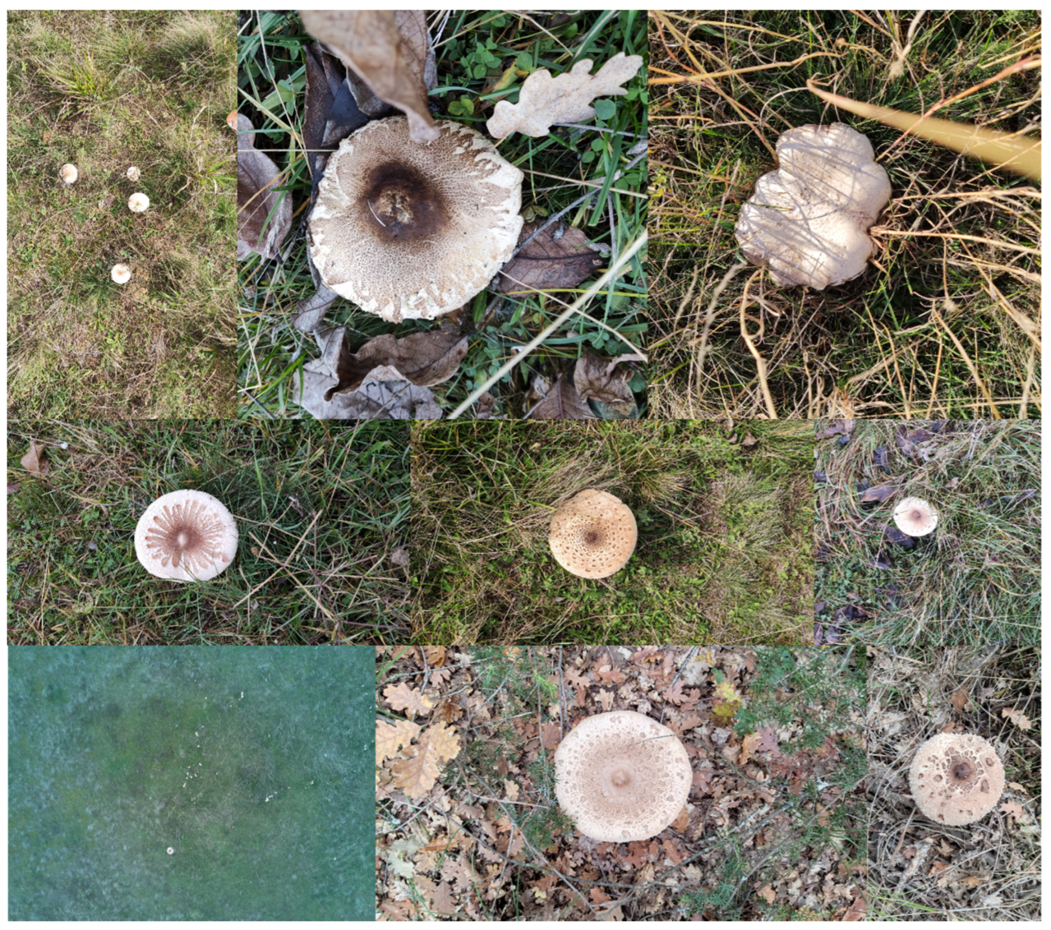
Figure 2.
Research territory in the western part of the Macedonia region of Greece.
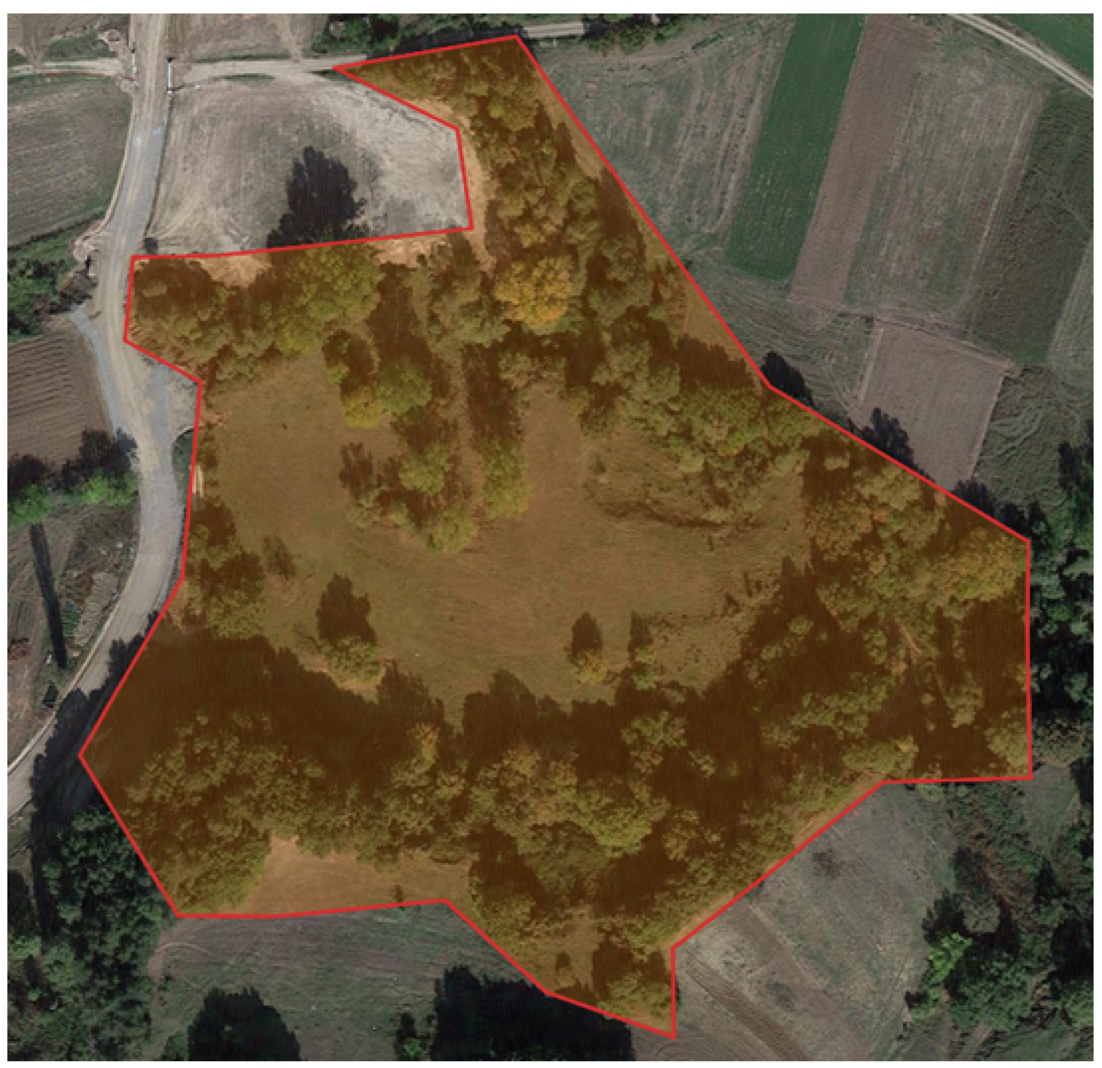
Figure 3.
Building and assembling a drone with low-cost 3D materials and equipment.
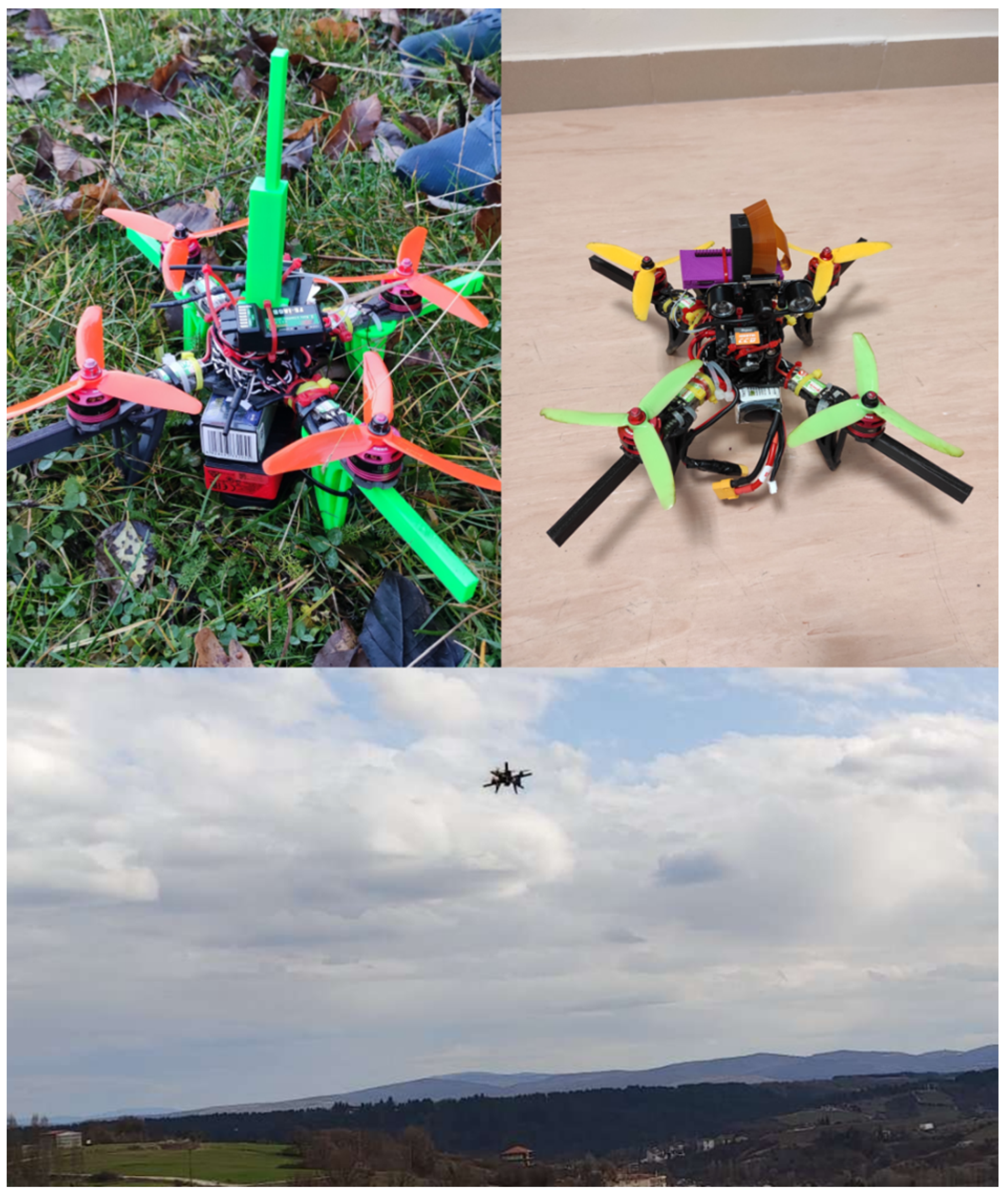
Figure 4.
Statistical outcomes of the OMPES and WOES dataset: (a) bar chart of the number of objects in each class; (b) normalized target location map; (c) normalized target size map.
Figure 4.
Statistical outcomes of the OMPES and WOES dataset: (a) bar chart of the number of objects in each class; (b) normalized target location map; (c) normalized target size map.
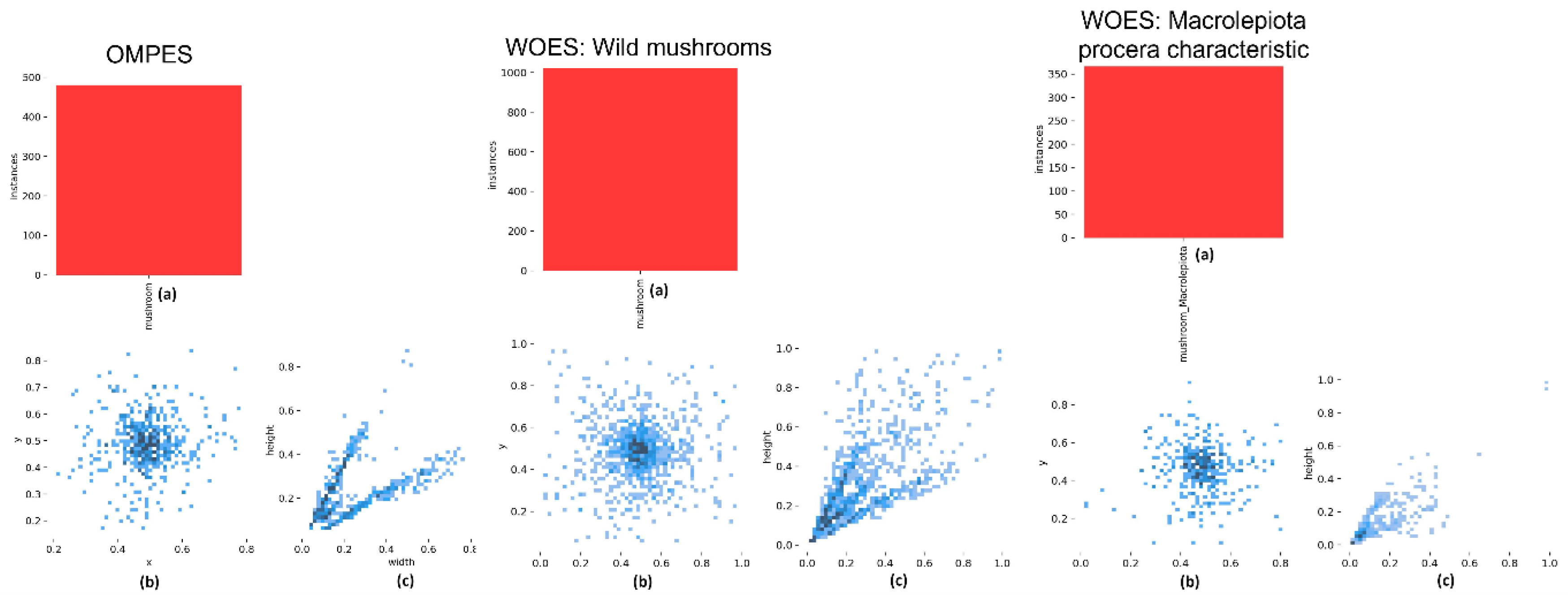
Figure 5.
The five spectral bands: (a) GREEN; (b) NIR; (c) RED; (d) REDEDGE and (e) RGB.
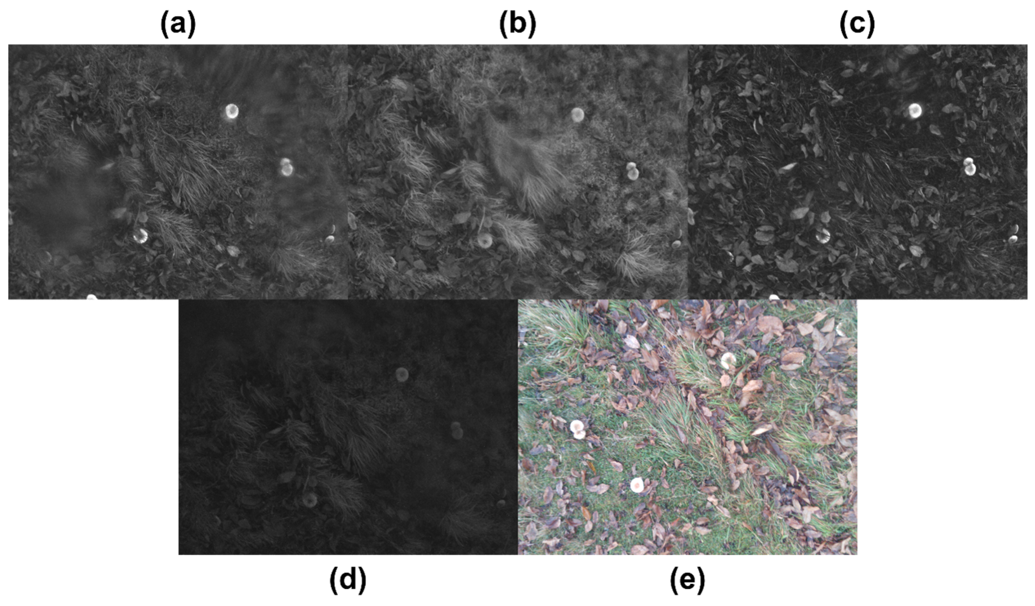
Figure 6.
Example of two raw spectral bands: (a) NIR and (b) RED.
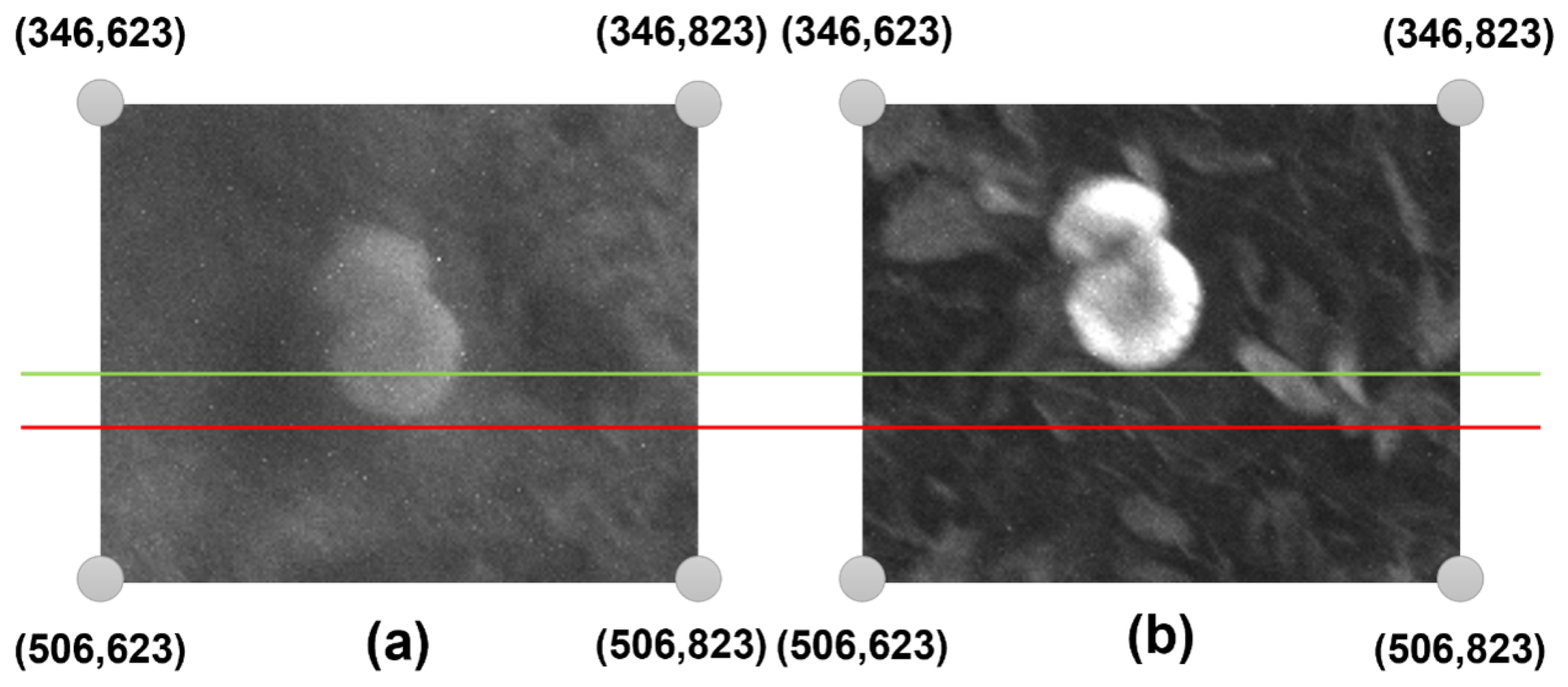
Figure 7.
The four raw spectral bands are (a) GREEN; (b) NIR; (c) RED; and (d) REDEDGE. The four processed spectral bands are (e) GREEN; (f) NIR; (g) RED; and (h) REDEDGE with frequency thresholds. Finally, the RGB (i) is edited manually by researchers in order to indicate the ground truth of wild mushrooms (orange boxes).
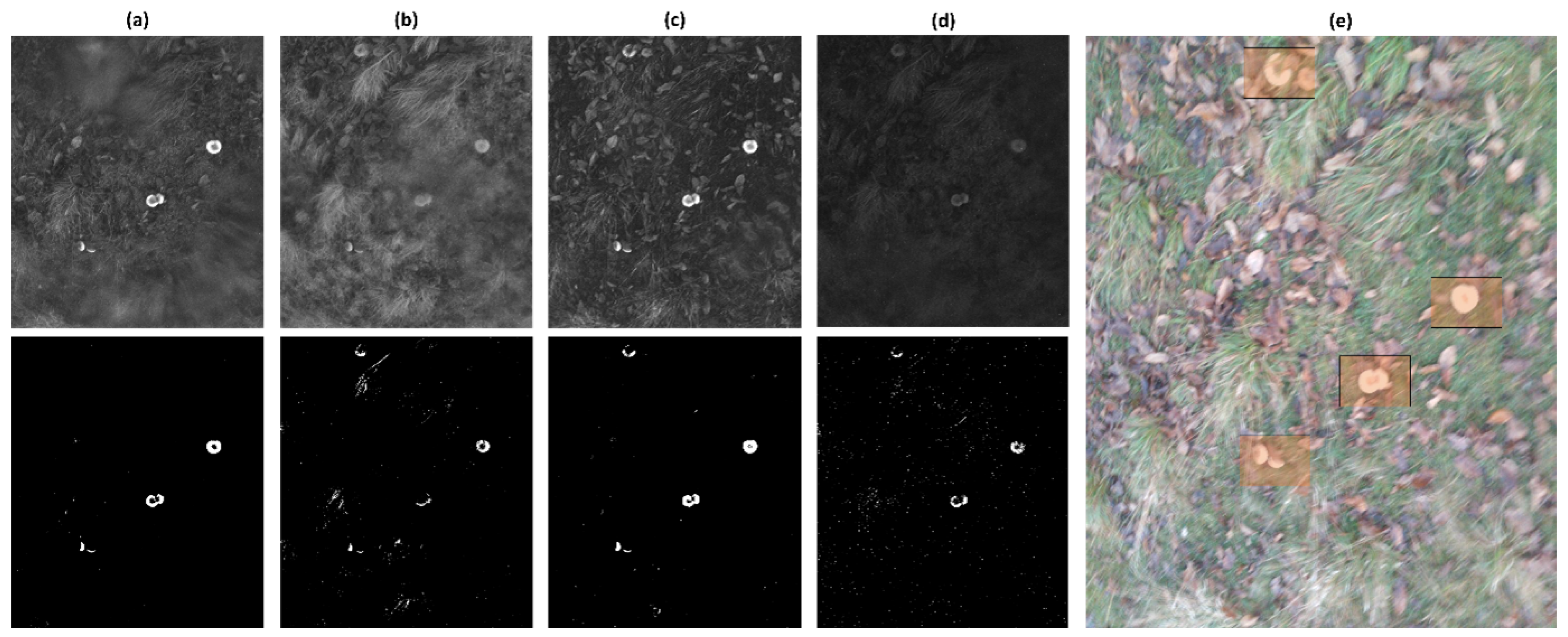
Figure 8.
The suggested architecture consists of many components: a) phase one, b) phase two, c) a base station, and d) a drone operator.
Figure 8.
The suggested architecture consists of many components: a) phase one, b) phase two, c) a base station, and d) a drone operator.
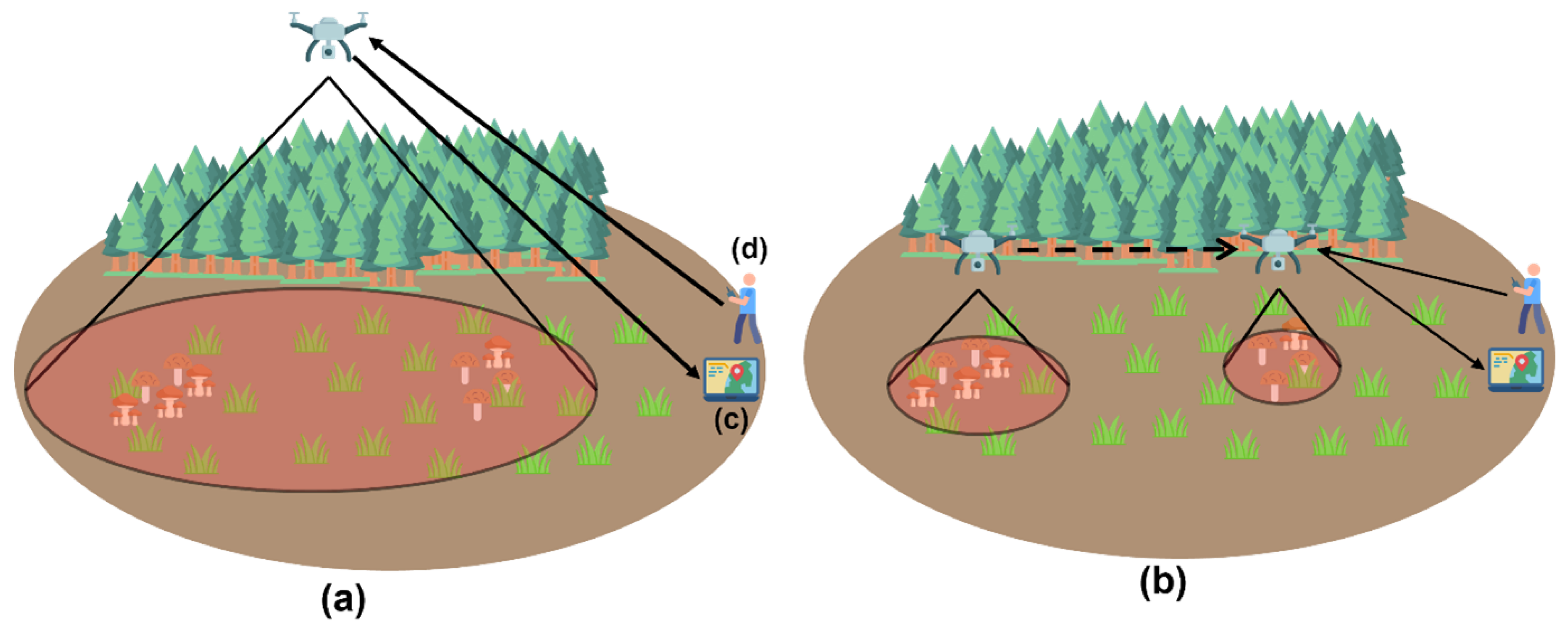
Figure 9.
An example of vegetation indices is from a multispectral image camera taken at a height of 60 metres. The three vegetation indexes are a) NDVI, b) OSAVI, and c) NDRE. Also shown is d) the RGB spectrum image.
Figure 9.
An example of vegetation indices is from a multispectral image camera taken at a height of 60 metres. The three vegetation indexes are a) NDVI, b) OSAVI, and c) NDRE. Also shown is d) the RGB spectrum image.
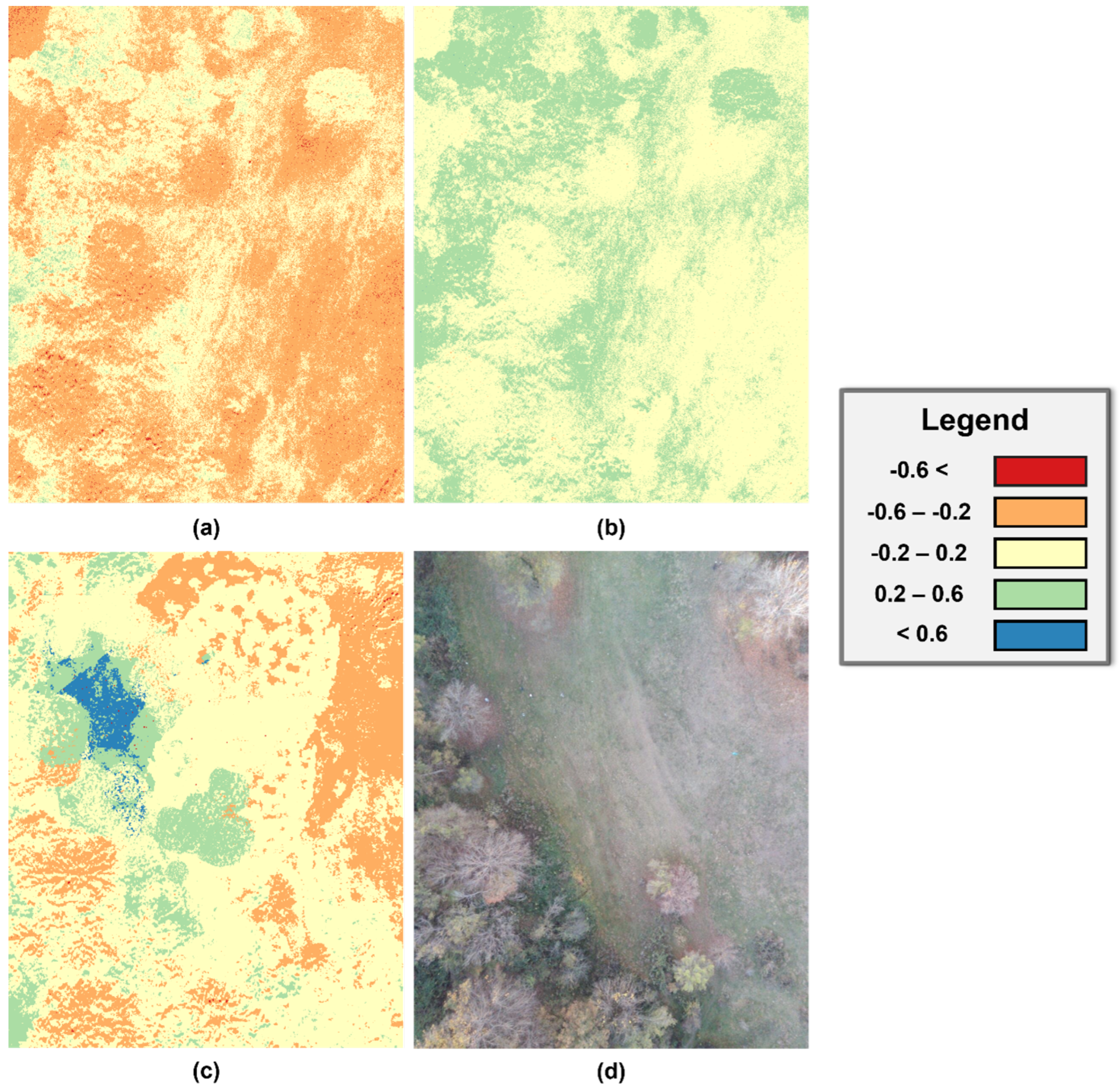
Figure 10.
The output images are a) HighValueSpots, b) BlurredHighValueSpots, c) GroupedBlurred- HighValueSpots, d) ContourGroupedBlurredHighValueSpots, and e) MushroomLocations.
Figure 10.
The output images are a) HighValueSpots, b) BlurredHighValueSpots, c) GroupedBlurred- HighValueSpots, d) ContourGroupedBlurredHighValueSpots, and e) MushroomLocations.
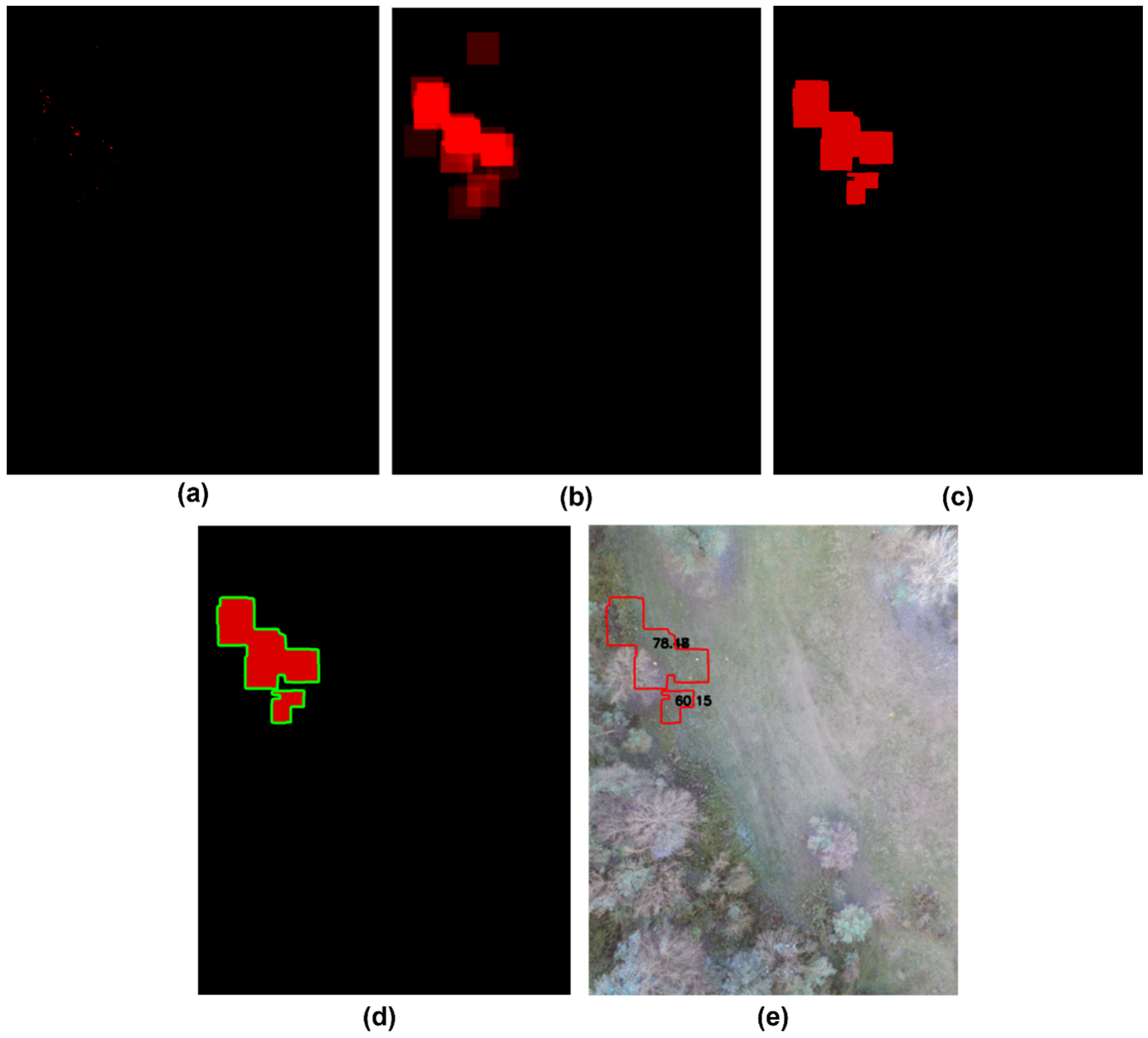
Figure 11.
Pipeline of phase two.
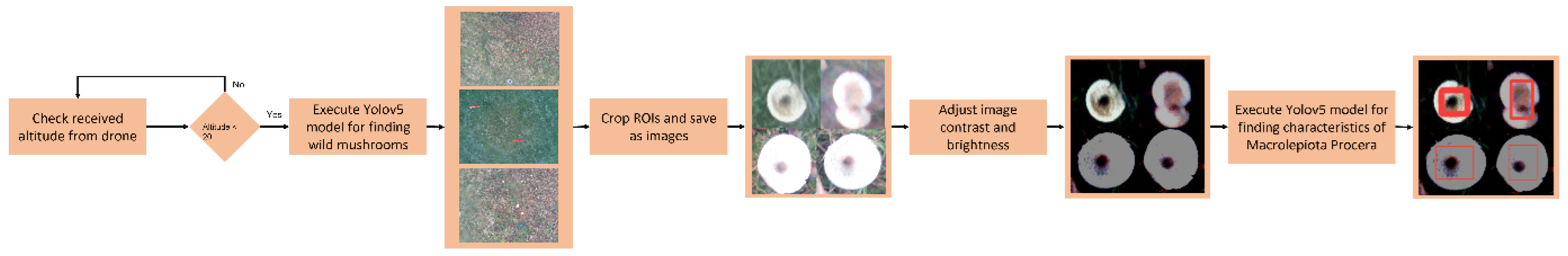
Figure 12.
Confusion matrix for the dour models: a) WildMushroom model with default hyperparameters, b) Wildhyperparameters model with evolves hyperparameters, c) Characteristic Procera model with default hyperparameters, and d) Characteristic Procera model with evolves hyperparameters.
Figure 12.
Confusion matrix for the dour models: a) WildMushroom model with default hyperparameters, b) Wildhyperparameters model with evolves hyperparameters, c) Characteristic Procera model with default hyperparameters, and d) Characteristic Procera model with evolves hyperparameters.
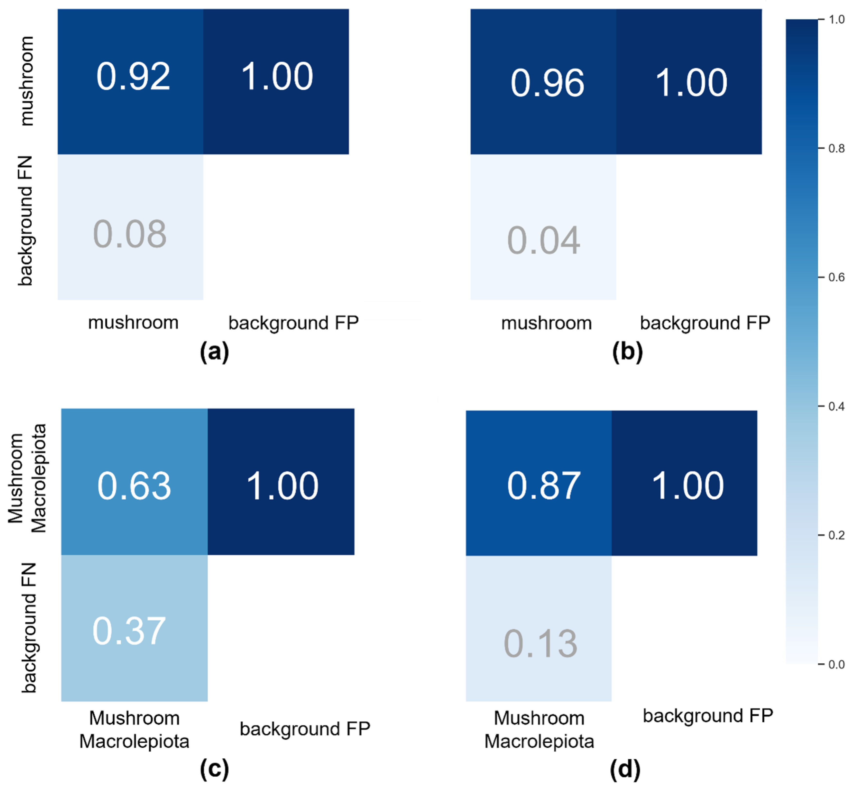

Table 1.
Parameters for the processing of multispectral images.
| Band | Left | Up |
|---|---|---|
| NIR | 16 | 24 |
| RED | 35 | 15 |
| GREEN | 29 | 2 |
| RGB | 21 | 20 |
Table 2.
Frequency ranges in multispectral images that are most suited for identifying wild mushrooms.
Table 2.
Frequency ranges in multispectral images that are most suited for identifying wild mushrooms.
| Band | Lower Threshold (kHz) | Upper Threshold (kHz) |
|---|---|---|
| NIR | 38 | 40 |
| RED | 37 | 39 |
| GREEN | 38 | 40 |
| RGB | 16 | 18 |
Table 3.
Training hyperparameters.
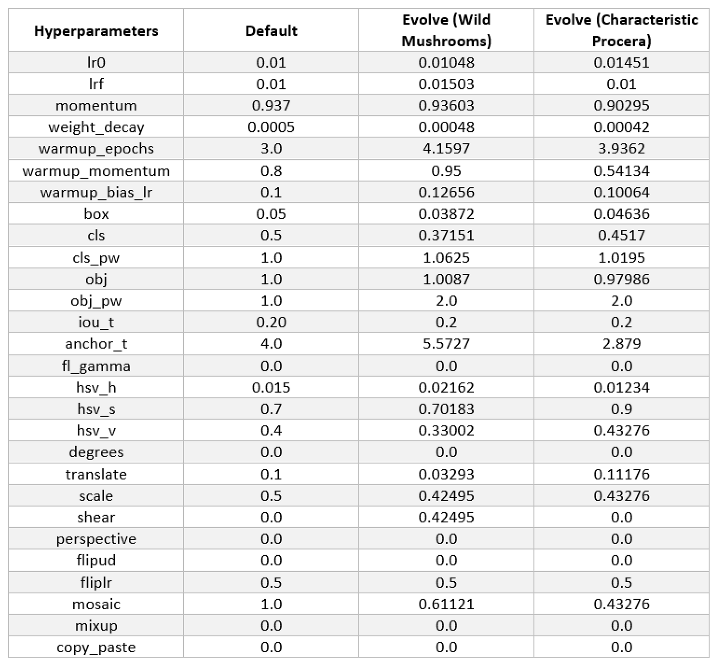
Table 4.
Results of machine learning models.
Disclaimer/Publisher’s Note: The statements, opinions and data contained in all publications are solely those of the individual author(s) and contributor(s) and not of MDPI and/or the editor(s). MDPI and/or the editor(s) disclaim responsibility for any injury to people or property resulting from any ideas, methods, instructions or products referred to in the content. |
© 2025 by the authors. Licensee MDPI, Basel, Switzerland. This article is an open access article distributed under the terms and conditions of the Creative Commons Attribution (CC BY) license (http://creativecommons.org/licenses/by/4.0/).
Copyright: This open access article is published under a Creative Commons CC BY 4.0 license, which permit the free download, distribution, and reuse, provided that the author and preprint are cited in any reuse.


