
Submitted:
11 April 2025
Posted:
16 May 2025
You are already at the latest version
Abstract
This technical report explores various methods for characterizing the complexity of strings, focusing primarily on Algorithmic Complexity (AC), also known as Kolmogorov Complexity (K). The report examines the use of lossless compression algorithms, such as Huffman Coding and Run-Length Encoding, to approximate AC, contrasting these with the Coding Theorem Method (CTM) and Block Decomposition Method (BDM) approaches. We conduct a series of experiments using leaked passwords as data, comparing the different methods across various alphabet representations i.e.: ASCII and binary. The report highlights the limitations of Shannon Entropy (H) as a sole measure of complexity and argues that AC offers a more nuanced and practical approach to quantifying the randomness of strings. We conclude by outlining potential research avenues in areas such as source coding, cryptography, and program synthesis, where AC could be used to enhance current methodologies
Keywords:
information theory
; algorithmic information theory
; resource-bounded Kolmogorov complexity
; algorithmic complexity
; CTM
; BDM
; randomness
; source coding
; lossless compression
; Huffman coding
; run-length encoding
1. Introduction
In this work, we analyse and investigate different approaches to characterize a string’s complexity. Indeed, a number of measures and metrics have been developed; we list a number of them in our literature review. However, the focus of this work will revolve around Algorithmic Complexity (AC) also known as Kolmogorov Complexity (K). The reasons for this selection will be exposed and motivated hereafter.
The use of Kolmogorov Complexity (K) has for too long been confined to theoretical studies and exploration. In this work, one of our goals is to showcase the practical side, the power and versatility of Algorithmic Information Theory (AIT). Kolmogorov Complexity is one of the component of this field and it can be used to quantify the degree of randomness in an object/string. Randomness can be characterized distinctively for infinite sequences. However, in our setting we are interested in finite sequences or strings. Within this case, randomness can be distinguished only to some degree but not in an absolute form.
In this work, one of our goal is to present a different perspective to approximate Kolmogorov Complexity (K). Indeed, the latter has often been approximated using tools from lossless source coding. As a matter of fact, the use of lossless compression tools for text based information prevents altering or losing the nature of the underlying concept/idea/information; this contrasts with lossy compression schemes.
The conducted computations allow us to broaden the surface area of Algorithmic Information Theory (AIT) practical applications. In order to achieve that, we make use of the Coding Theorem Method (CTM)/Block Decomposition Method (BDM) methods which allow to approximate the Algorithmic Complexity of an object; which is known to be theoretically uncomputable.
To get a grasp as to how the approximation based on CTM/BDM behaves with respect to lossless schemes, we use it in a comparative setting that includes Huffman Coding (HC) and Run-Length Encoding.
2. Our Contributions
In this work, we study one dimensional objects i.e. finite/bounded strings. We are interested in deriving practical results/insights from the use of Algorithmic Complexity (AC) also known as Kolmogorov Complexity (K)1 with respect to Shannon Entropy (H). More specifically, our work bridges closer the gap between the theory and practical side of approximated Algorithmic Complexity.
In the pursuit of these objectives, we make the following contributions:
- We analyze the effect of the alphabet size (used to encode the string) has on the compression ratio(Cr) on the selected lossless compression schemes i.e.: Huffman Coding (HC), Run-Length Encoding (RLE).
- We conduct comparative analyses between Shannon Entropy and Algorithmic Complexity with regards to the randomness character of a finite string (Section 5.2).
- In order to approximate the Algorithmic Complexity of bounded strings, we propose an approach to overcome the current limitation of the CTM/BDM (Section 5.2.2).
- We propose an alternative method to approximate Shannon Entropy (H) in the software package pybdm ([1]). This is an implementation of the Schürmann-Grassberger estimator (7). The added value of this approach is that, it is bias minimized compared to the maximum likelihood approximation method (Section 5.2.1).
3. Related Work
In this section, we outline a number of complexity measures that have been worked out. Some of the them well known while others to a lesser degree. Moreover, some of the complexity measures are more grounded in physical reality(or at least consider their feasibility) i.e. that the function is effectively computable. While other approaches evolve solely on a theoretical level.
We position ourselves between the two approaches i.e.: building a bridge between theoretical work and practical aspirations. In other words, we are interested in a resource bounded information-theoretic approach to complexity. We consider the study of finite strings and are constrained to resource bounded approaches. The latter follows of the will to have quantifiable results with arguably improved quality over entropy-based approaches.
Even though some work have been developed in a purely theoretical form, they bring guarantees(bounds) and guidance when making practical considerations. Furthermore, through this work we would like to illustrate that the undecidability of Algorithmic Complexity (AC) can be approximated by at least another method that lossless compression techniques. Hereafter follows a selected number of complexity measures that can be used to characterise a finite string’s complexity. That is because most entropy-based measures deal with probability distributions whereas Kolmogorov complexity with individual objects.
Shannon’s seminal paper: A Mathematical Theory of Communication, ([2]) has led the foundations of a plethora of works in different fields. Some of these inspired from it, while others building upon by generalizing on it e.g., Rényi Entropy (RE), ([3]). Nevertheless, these visions do not coincide with our object of study i.e. characterising finite strings complexities.
In ([4]), the concept of logical depth is formalized. Among other elements, it is argued that the value of a message does not lie in its “information” per se but within the part that requires computational2 work - without this work being trivial. This notion of depth is crystallised under a mathematical definition that favors programs with a faster run-time by means of a “harmonic mean”. In other words, a string has a large depth if it has a short program and which is also computationally demanding.
A closely related theory to the aforementioned logical depth is computational depth defined by ([5]). Intuitively, computational depth measures the "nonrandom" information in a string. In that work, they develop this notion in three flavors:
a) Basic Computational Depth, b) Sublinear-time Computational Depth, c) Distinguishing Computational Depth.
The definition a) contrasts with C. Bennett’s logical depth in that they do not require a parameter called “s-significant” which is tied to the least time required by universal Turing machine to compute the string by a program. They actually build into their definition of computational depth a similar concept which penalizes the run-time of a program. The two other concepts/definitions are really interesting but beyond the scope of the current work.
Another correlated notion is the one of sophistication ([6]), first introduced by M. Koppel. Similarly to depth, it measures the “nonrandom” information in a message. They relate computational depth and sophistication by showing that strings with maximum sophistication are the deepest of all strings. Where logical depth deals with program run-times, sophistication is concerned with program lengths.
Additionally, another interesting entropy-based measure is the so-called Deng Entropy and its improved version: ([7]). It is also a generalization of Shannon Entropy in the framework of Dempster-Shafer theory. It was introduced to quantify the level of uncertainty in the basic probability assignment in Dempster-Shafer theory ([8]).
Furthermore, for some of the measures, we can notice that despite its central position, Shannon Entropy position has to be considered within the context of the applied field. This aspect will be of concern and developed later on.
As mentioned in the Introduction Section 1, we are concerned and make use of the Algorithmic Complexity (AC) approach to bounded string complexity; which will be exposed in Section 4.2.
4. Theoretical Landscape
In this section we give a high level overview of the field of Algorithmic Information Theory (AIT); which is characterised by G. Chaitin [9] in a few words as:
AIT = recursive function theory + program size [9]
Figure 1.
Algorithmic Information Theory - main components.
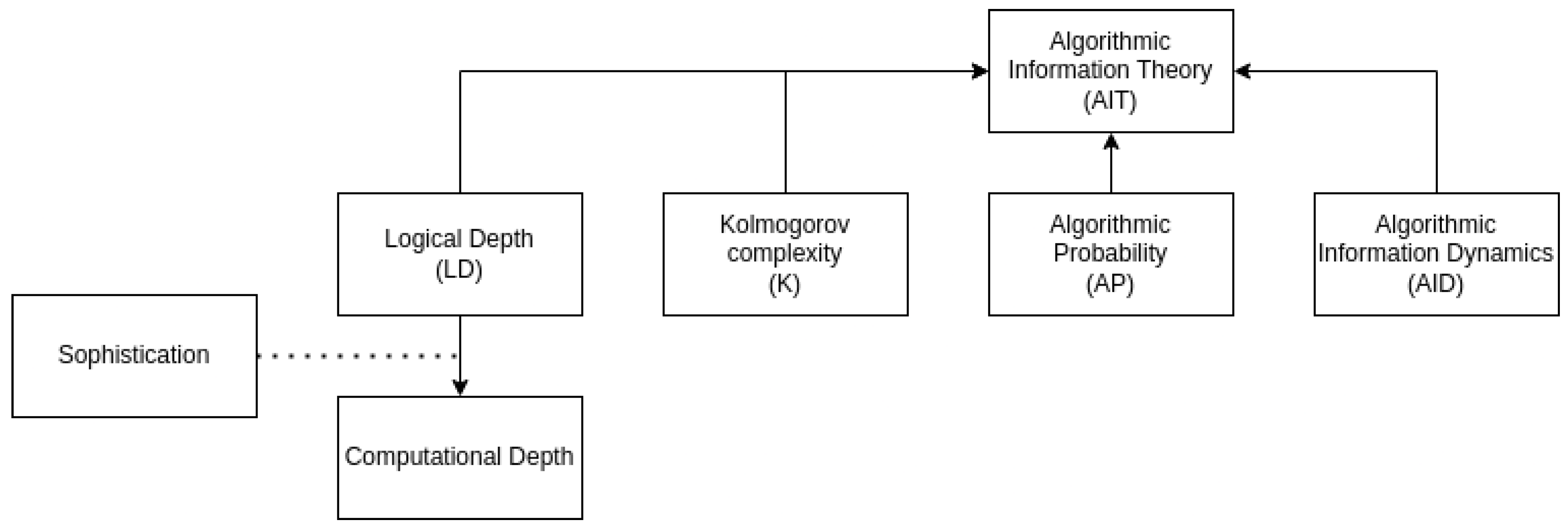
This work uses prefix Kolmogorov’s complexity which is made computable by approximating the algorithmic probability, also known as Levin’s semi-measure3.
Similarities exist between Information Theory (IT) and Algorithmic Information Theory (AIT), we outline some of them hereafter. Even though developed for telecommunication purposes, Shannon’s entropy ([2]) has seen applications in plethora of domains e.g., physics, computer science, biology and many more.
One of the discrepancies between them is that, AIT considers the information in a single object. Whereas in information theory we deal with random variables belonging to a probability distribution. We posit that the information theory body work can be used as a basis in the field of algorithmic information theory. A number of works favoring this hypothesis can be found in: ([10,11,12]).
In the spirit of Wigner’s essay: The unreasonable effectiveness of mathematics in the natural sciences ([13]), in Compression is Comprehension, and the Unreasonable Effectiveness of Digital Computation in the Natural World ([14]) further develops Chaitin’s notion that compression is comprehension and proposes two approaches to the nature of the world: algorithmic or random.
The notion of compression, compressibility or incompressibility is a cornerstone in characterising the randomness of a string. Indeed, based on Kolmogorov’s complexity a string is said to be maximally random if its shortest representation is the length of the string itself – its information content is maximal. We thus push the notion of compression further by stating that to some degree: to compress is to predict, to model.
A great deal of information about the previous three pillars of Algorithmic Information Theory can be found in the following resources:
In the following sections we will outline some of the theoretical specifics that will help us to approximate a string’s Algorithmic Complexity (AC) or Kolmogorov Complexity (K).
4.1. Dealing with Kolmogorov’s Complexity Uncomputability
The body of work concerning the field of Algorithmic Information Theory (AIT) has received little attention in general; and especially from an application/practical perspective.
At least, two attitudes can be taken when faced with the uncomputable nature of Kolmogorov’s complexity: to bow in front of the theoretical bounds or trying to bypass/overcome it in some way e.g.: trying to be creative.
Indeed, the Halting Problem (HP) is a challenging one. We argue and show that, if we change our position this can be used as a feature; somehow in the spirit of numerical algorithms. One perspective is to approach it as an anytime algorithm which means that we can always get better approximations.
The Kolmogorov complexity of a string s is defined as follows:
Which reads as: the Kolmogorov Complexity (K) of a string s is the length with respect to a reference Turing machine T of the shortest input p when fed to the machine T and produces the string s.
It is to be noted that the randomness of a finite string can only be approximated to a certain degree i.e. not with an absolute precision.
Definition 1
([17]). A string s is random iff K(s) is approximately equal to . An infinite string α is random iff .
The invariance theorem ([18], p.39) guarantees that the length of the self-delimiting program generating the string of interest is bounded up to a constant c - based on its respective reference machine(which is by the definition a universal one).
4.2. Approaches to Approximating Algorithmic Complexity
As discussed, we are interested in applying Kolmogorov Complexity to bounded sequences or strings.
We identify and list four main lines of practical approaches to approximate Algorithmic Complexity:
In this work, we explore in Section 5.2 the behavior of these approaches: (i), (ii) and (iii).
Huffman coding(i) and run-length encoding(ii) belong to the cluster of lossless compression algorithms.
The approach(iii) exploits the relation between:
- the frequency of occurrence of a string(through Algorithmic Probability (AP))
- to its Algorithmic Complexity (AC).
The link is made by rewriting Levin’s coding theorem ([23]) or also known as algorithmic coding theorem which leads to the Coding Theorem Method (CTM). This point is developed in Section 4.2.3 followed by its extension Block Decomposition Method (BDM) in Section 4.2.4.
In the following sections, we briefly introduce the two lossless compression techniques. As a matter of fact, Huffman Coding and Run-Length Encoding have been studied extensively. We will therefore emphasize some key elements, properties and, suggest the curious reader to refer to the literature for a detailed description.
Interestingly, it has been theorized, empirically observed, that a lower limit for lossless compression schemes are bounded by Shannon’s source coding theorem. However, a review of the literature seems to hint that this might not hold for every object type. This point is further developed in Section 4.3.
Regarding the Coding Theorem Method (CTM) and Block Decomposition Method (BDM), we expose their core components; which gives a good grasp as to their inner workings.
4.2.1. Run-Length Encoding
The Run-Length Encoding (RLE) is a content dependent lossless compression scheme. The algorithm works as follows: it replaces the consecutive occurrences of a symbol by a single code followed by the number(integer) that this symbol appears. It is a widely used algorithm because of its simplicity and speed.
Therefore, it performs best when it is confronted with data that has consecutive repeated symbols in it. An example in a two dimensional setting can be an image describing something with minimal variation in it. In this context, the simple Run-Length Encoding algorithm is able effectively compress i.e. to reduce the size of the original data.
However, if the data contains very little or no repetitions/regularities then, Run-Length Encoding’s compression can end up being bigger than the original data. This is known as the size-inflation issue and can be handled in various ways e.g.: through a two passes scheme, the use of heuristics ([24]).
4.2.2. Huffman Coding
The Huffman Coding (HC) algorithm is an optimal lossless statistical compression scheme. It builds variable length codewords5 and assigns the shortest codewords to the most frequent symbols.
Huffman coding has been shown to be optimal for a prefix binary code (). The optimality is guaranteed by Lemmas [1.1.12, 1.1.13] and Theorem [1.1.14] - ([26] p.10).
Part of the motivation for its widespread use are: a high compression ratio(i.e. approaching the entropy limit6) and simple implementation possibilities. However there is a requirement for the Huffman encoding to operate: it is to have access to the source statistics, or an approximation of it.
This shortcoming can be dealt with by using two passes on the data. A first pass to construct the frequency distribution and, the second path to proceed with compression. This is the strategy behind the adaptive Huffman encoding scheme.
In the experimentation, our focus targets the classical Huffman Coding (HC) algorithm. This is motivated by the fact that we want to observe and compare the compression ratios(Cr) and entropy7 of the selected algorithms: HC, RLE, CTM/BDM.
Reference work
introducing the Huffman Coding algorithm: ([27])
4.2.3. Coding Theorem Method - CTM
The roots of the Coding Theorem Method (CTM) can be trace back to ([28]), it takes the following form:
One of the main challenge is to find a way to estimate Levin’s semi-measure . Using the Coding Theorem Method (CTM) this is achieved through an exhaustive search of Turing machines whose halting runtimes are known i.e. Busy Beaver Machine - BBM ([29]). This will be used to build a probability distribution which in turn can be used to approximate K(s). Levin’s semi-measure(also called the universal distribution) which is approached by running small Turing machines and measuring the frequencies of generated strings.
A probability distribution of the occurrence of bitstrings is generated by running five states and two symbols busy beaver functions. This will construct the empirical distribution which is the estimation of the algorithmic probability (AP or ). At the end of the process, using CTM, we get an approximation of the Kolmogorov Complexity (K) or Algorithmic Complexity (AC) of a bitstring s.
4.2.4. Block Decomposition Method - BDM
The Block Decomposition Method (BDM) is an extension to the CTM. If we are interested in getting the Algorithmic Complexity (AC) of bitstring greater than twelve in length then we have to consider the use of the Block Decomposition Method (BDM). Indeed, the Kolmogorov complexity of long bitstrings becomes quickly intractable. To overcome this computational explosion, BDM follows a divide and conquer kind of approach.
From ([33] p.14), the BDM of a string is given by:
In essence, BDM consist in slicing a sequence into smaller pieces so that we can benefit from the computation that has been done for CTM. It is to be noted that the worst case estimation of K by BDM will be as good as Shannon’s block entropy.
Reference works
4.3. Bounds - Entropy
It is a well implanted theoretical result that Shannon’s source coding theorem ([2,34]) sets a lower bound for lossless compression algorithms. It establishes a global minimum as to how much the data can be compressed down to without loss of information.
This constitutes one of the reason for not taking into account lossy data compression schemes. Even though, they can go beyond the theoretical limit, we want to be able to compare the compression ratio to the original information content.
In this work, we express it through Rényi Entropy (RE), which is a generalization of Shannon Entropy. It is a one-parameter() information measure. It is defined ([3]) as follows:
with , where X is a discrete random variable which can take n possible outcomes and is the probability of event x.
where is called the order of Rényi Entropy.
The case where yields Shannon Entropy also known as first-order Shannon Entropy:
Besides in practice, it is not always possible to have access to the average codewords lengths. Based on theoretical results, we can however predict the Compression ratio (Cr) limits.
Nevertheless, recently this theoretical bound is being challenged. Empirical research conducted on images in ([35]) suggests that structural information about pixels of an image can not be captured solely by statistical approaches.
A first-order entropy does not consider the context within the neighbouring of a pixel. One can reason about this similarly to the way Convolutional Neural Network (CNN) filters exploit spatial locality. The assumption of a degree of dependence between pixels or inductive bias, constitutes one the strengths of CNN and their performance in Computer Vision (CV).
Furthermore, the behavior of Shannon Entropy and Algorithmic Complexity on graphs are investigated in ([36]). Among other elements, this study exposes that the application of Shannon Entropy better behaves, is more sensical if context is taken into account.
Indeed, in first-order Shannon Entropy, the probabilities of random variables are independent of each other; which in the context of graphs is problematic because these have a precise structure. Additionally, H lacks an invariant theorem ([36]), a property that guarantees convergence of results(up to an additive constant) agnostic to the description language.
The aforementioned elements lead us to articulate that despite its foundational aspect Shannon Entropy (H) has to be considered/modulated in light of the object under study.
4.4. The Reference Machine Question
The theoretical result given by the invariance theorem(2) guarantees that whatever the reference universal Turing machine is, we will face a difference of at most a constant c.
For resource-bounded Kolmogorov Complexity (K) and when considering applicable results; the reference question is central. This notion of reference starts, involves and can lead to the following:
- What model of computation? e.g.: Turing machine, -calculus, combinatory logic, boolean circuits…
- How does the alphabet/encoding affect computation?
Some questions that can rise: does it actually matter? What is the impact of the alphabet and encoding on the Compression ratio (Cr)? From theoretical perspectives it may not be big of deal i.e., they have been shown to be Turing-complete. For the different models of computation, the Church-Turing thesis/conjecture suggests that the computational power of these models are equivalent.
Nevertheless, if we consider that all models of computation can be reduced to the Turing machine, from a practical/resource perspective the question is more nuanced. Intriguingly, this can be thought of/linked to Wolfram’s principle of computational irreducibility [37], Ch.12, p. 737.
One of the characteristics and strengths of Algorithmic Complexity is that it allows a program independent specification of an object. Yet, in a resource-bounded Kolmogorov Complexity measure if one takes into account finite and limited resources(e.g., compute, memory…) then one might want to take advantage of every possible bit.
In our setting(CTM/BDM), the taken path to approximate Algorithmic Complexity is mainly time bounded. The induced precision loss caused by a too reduced allocated running time, is absorbed by the fact that most programs halt quickly or never do ([38]).
As mentioned in Sections CTM Section 4.2.3, BDM Section 4.2.4, these computational approximations methods rely on a reference universal prefix machine. The CTM exploits the link between the frequency occurrence of a string and its Algorithmic Complexity. Both Algorithmic Complexity and Algorithmic Probability work with respect to a reference Turing machine U.
We just mentioned that the description independence is a core feature of Kolmogorov Complexity. Nevertheless, according to ([39]) completely getting rid of the machine dependence is not feasible. In the field of Algorithmic Information Theory, the selection of the ”best” or most suited reference machine is still open question - if possible at all.
4.4.1. On the Power of Turing Machines
We build, make use of, evolve with digital computers. This has implications as how do we encode the information from what we experience as reality into our computing devices. Which raises the question about the nature of reality and therefore the mapping into our computing devices: analog, digital, nature-inspired computing(e.g., DNA based computing), quantum computing.
From these different models of computation naturally rise the question of their universality and, by extension their equivalences. Even though the definition of an algorithm does not make consensus, an axiomatic approach to the theory of computation allows us to prove their theoretic correspondence.
Turing machine model is often chosen to implement (computable) functions. Concretely, in a day-to-day setting this translates more closely to a finite-state machine(FSM) or finite-state automaton(FSA); this is because the Turing machine is an idealized model with features such as unbounded memory. Subsequently, making not easy to have a physical correspondence/implementation.
On the practical side i.e. when actually performing computation using an actual physical substrate, we often want those to be fast, efficient and reliable. The Turing machine model is simple but powerful ([40]) enough to render the notion of "what is it to compute" clear and convincing. However, from a practical perspective it is not efficient. Even multiplying tapes on the Turing machine model does not help much. Furthermore, it has been shown that multi-tapes are equivalent to single tape Turing machines ([41] p.213).
Could it be the case that universality in computation is more ubiquitous than what it appears at first sight? A number of works and conjecture might suggest so. Hereafter, we present a some of them.
One of the key ideas that transformed the early computing machinery into computers as we know them today is, mainly the concept of a stored program. More specifically, the ability to re-program the machinery without having to physically intervene i.e. using a software approach. This was formalized and have been known under the von Neumann architecture. It is the commonly known computer design paradigm but there are others e.g. Harvard architecture …
When the notion of a stored program collides with the question about effective computation i.e. as in real implementation; it raises the question about the expressive power of the machine model. This is where Turing-completeness comes into play. Informally, and from a high level perspective, a machine endowed with this property is able to compute everything that can be computed given reasonable8 time and space requirements.
The notion of Turing-completeness is also pivotal when characterizing the Algorithmic Complexity (AC) of an object. Indeed, the Algorithmic Complexity of an object is specified with respect to a Turing machine which by definition is a universal one. In Algorithmic Information Theory (AIT), Algorithmic Complexity is cursed with uncomputability. Earlier, we argued that this can be flipped to our advantage. However, in real world application, we prefer algorithms to be as efficient as possible. By pushing our thought process further about efficient computing and universality, we can ask ourselves the following: what are the requirements for a machine to hold the universal property? Or, do we actually need Turing-completeness in everything scenario?
All in all, in ([42]) the author addresses the question about the minimal instructions set that are required in order to gift a machine with universal computation capabilities.
Another element favoring the "reduced requirements hypothesis" is Wolfram’s -machine, with two states and three symbols has been shown to demonstrate universality ([43]).
4.5. Impact – What’s the added value of AIT?
The use(as in practical) of Algorithmic Information Theory (AIT) and, specifically Algorithmic Complexity casts new perspectives on the Information Theory (IT) corpus. As mentioned in Section 4 some similarities between AIT and IT can be drawn and exploited.
This is precisely what powers the Block Decomposition Method. Theoretical results ([33]) assure that in the worst cases it will behave like Shannon’s block entropy; otherwise it will provide more granular/refined results.
If a problem can be posed as a prediction one then it is possible to resort to Algorithmic Information Theory (AIT). In our setting, we are interested in quantifying the complexity of a string. That is, its degree of randomness, yet again its incompressible character.
Some advantages of using BDM are:
- Parameter-free method,
- Computationally efficient,
- Better encompasses the universal character.
Some of its shortcomings:
- Currently BDM’s approximation has been constructed using a two symbols or binary() alphabet,
- Its universal character.
5. Experimentation
In this part, we focus on applying the presented methods and listed in the next Section 5.2.
The objectives are twofold: weighing a string’s complexity through its approximated randomness. The impact of the encoding i.e.: the chosen alphabet used to represent the source input.
5.1. Data - Text Sequence
A natural candidate to conduct an analysis on strings is probably the most commonly used passwords collected from diverse leaks. Indeed, we are given sequences/strings that are collected from different sources; in a sense, the bias toward material selection is minimized.
When dealing with passwords10 and trying to understand their complexities, it is important to take into account the world of natural language. Naturally, passwords are dominantly composed of different character sets. Still, in most cases, humans anchor variations around a word or a composite of them. In order to have a better grasp about how to regard their complexities, we outline some elements pertaining to the study of natural language.
In the fields of linguistics, computational linguistics, one important question concerns the complexity of languages between them. In other words, are some natural languages more complex than others?
To characterize something as complex or the lack thereof, a measure(s) of some sort is(are) required. In natural language, complexity analyses can be conducted along the following axes: phonology, syntax, morphology, semantics and lexicon, pragmatics ([44] p.15).
The question about the equivalence between languages has been crystallized under the equi-complexity hypothesisby C. Hockett ([45]). It argues that complexities between languages are about equal to each other.
If the morphological and syntactical complexities are considered, the underlying mechanism that enables this levelling is called the trade-off hypothesis. This can be comprehended as follows: in most cases, if a language exhibits high morphological complexity it will have low syntactic counterpart; and vice-versa ([45]).
In a similar vein ([46]) conduct a large scale study concerning how information is structured in languages. Their quantitative analysis supports that languages prominently relying on word order rely less on morphological information.
([47]) identify and test a number of different morphological complexity measures e.g.: information in word structure(WS), word and lemma entropy(WH, LH). Some of them are derived from the field of information theory - Shannon Entropy. They observe a positive correlation between the different measures.
The previously outlined elements were just a glimpse into the world of linguistic and tangent fields. Nonetheless, we can observe that information-theoretic methods permeate different domains. Still, for entropy-based/derived measures, two aspects need to be taken into account. First, in order to be computed one has to have access to the underlying probability space governing the phenomenon of interest; this can be approximated by different means. Second, mirroring Algorithmic Complexity (AC) which studies individual objects, Shannon Entropy (H) quantifies a random object drawn from the probability distribution.
([44]) explores the Kolmogorov Complexity (K) approach to linguistic complexity; the taken path makes use of lossless compression algorithm i.e. gzip. However, lossless compression algorithms deliver an upper limit to K and, do not work well for short strings.
Incidentally, throughout this work, we make use of the word information or information content. Nowadays, this term is used for anything and everything. A formal definition is provided by ([47]) taken verbatim as follows:
Definition 2
(Information content measure). A partial function I from strings to is an information content measure if it is right-c.e.11 and is finite.
Additionally, also as being one of the instigator of the AIT field, ([48]) proposed a definition of information. With this initiative, he wanted to re-found the bases of probability theory based on the theory of recursive functions ([48,49]).
One of the key takeaways is that having a "self-contained", universal measure is a hard problem. This is similar to the requirements for universal source coding or data compression. To the best of our knowledge, the Kolmogorov Complexity approximation based on Algorithmic Probability is one of the few existing practical measures satisfying these requisites.
On an empirical level, enriched with the aforementioned elements, we decided to use a list of leaked passwords provided by NordPass12. They have compiled and extracted the two hundred most commonly used passwords from 4.3TB of data ([50]).
5.1.1. Preprocessing and Computing
We assumed the data(Section 5.1) to be ready-to-use so to speak. Nevertheless, we found three passwords that have duplicate instances/rows13: ’123456789’, ’000000’, ’987654321’.
This brings the number of unique strings to 197 in place of the initial 200.
Additionally, for reasons explained in the Section 5.10, the number of usable strings for comparisons between all algorithms outputs will be reduced to 173.
5.2. Methods
As described in the Section 4.3, we can only approximate to a certain degree the randomness of a bounded string. The choice of the reference machine and the encoding to represent the string has a direct impact on its quantified approximated Algorithmic Complexity (AC).
In this section, we put to the test the presented algorithms i.e.:
- Run-Length Encoding (RLE) - ∈ entropy coding, lossless compression [Section 4.2.1]
- Huffman Coding (HC) - ∈ entropy coding, lossless compression, [Section 4.2.2]
- Coding Theorem Method (CTM) / Block Decomposition Method (BDM) - custom built around Algorithmic Probability [Section 4.2.3, Section 4.2.4]
For each of the aforementioned algorithms, we proceed as follows:
- Apply the RLE, HC, CTM/BDM algorithms on the strings; if possible, in their ”native”/default representation - usually using an alphanumeric character encoding.
- Apply the three algorithms on the passwords in their binary representation
- Outline and compare the results
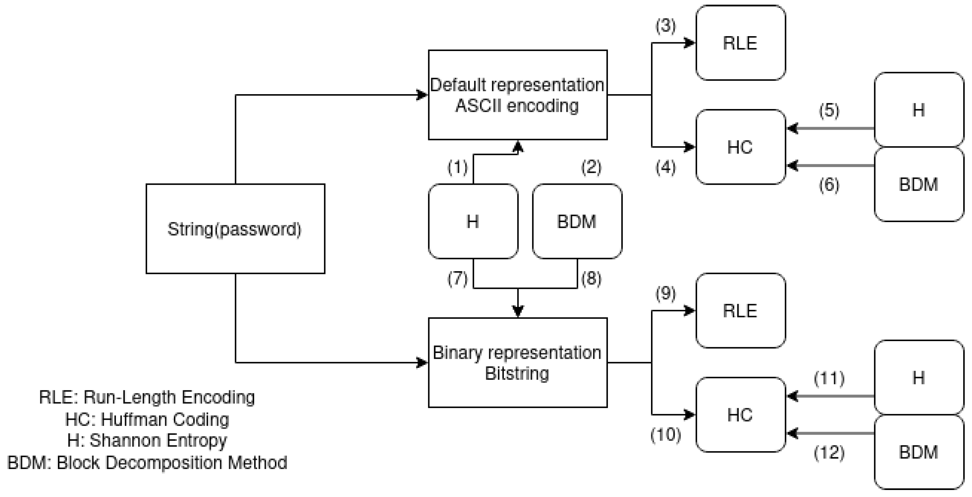
Figure 2.
Experiment Workflow.
5.2.1. On Computing Entropy
A number of approaches have been developed to compute Shannon Entropy. The two main approaches that stand out are based on: 1) the maximum likelihood estimation(MLE)14 and 2) using Bayesian approximation ([51]).
In a series of papers: ([52,53,54]) similar approximation methods are developed. This eventually shaped the Schürmann-Grassberger estimator ([55]). The added value of this approach is that it can be maximally bias minimized.
From ([54]):
where
We contribute an implementation of this approach through the pybdm ([1]) software package.
5.2.2. On computing BDM
By ASCII encoding, we mean a string under the usual form: abcd. The word string and ASCII is used interchangeably.
From ([56]):
ASCII code. The standard character code on all modern computers (although Unicode is becoming a competitor). ASCII stands for American Standard Code for Information Interchange. It is a (1+7)-bit code, with one parity but and seven data bits per symbol. As a result, 128 symbols can be coded. They include the uppercase and lowercase letters, the ten digits, some punctuation marks, and control characters.
Our objective is to compute the approximated Algorithmic Complexity (AC) through the Block Decomposition Method (BDM) of an object which in this case is a string under the ASCII format. However, BDM which is based on Coding Theorem Method has been computed for binary codes i.e. with an alphabet solely constituted of .
We circumvent the current BDM shortcoming by converting the ASCII encoded strings into their binary form. Using this technique, we are able to measure the approximate Algorithmic Complexity of the string(in this case we work with passwords).
5.3. Strings Under Their Default Alphabet Representation
In this section, we follow the workflow exposed in Figure 2 and report our results.
5.3.1. (1) - Shannon Entropy applied to strings
We start by computing the Shannon Entropy of strings.
An excerpt of some values:
696969 1.7913941946557577
Liman1000 2.133632995966046
asdf1234 2.017457140896491
147852369 2.1960370829590756
asd123 1.7270050849709604
Figure 3.
Histogram: Shannon Entropy - scipy.
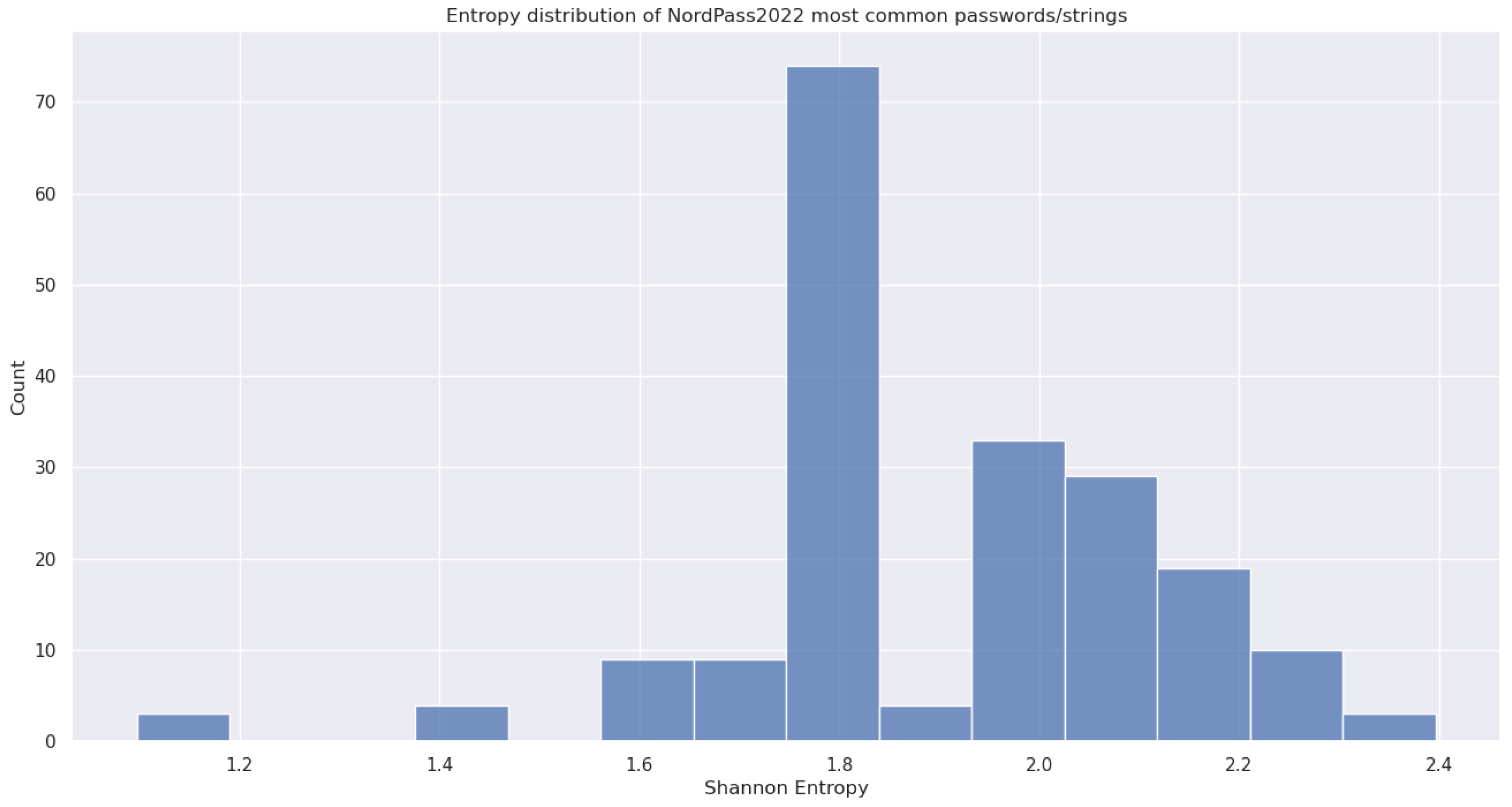
On the x axis, we have the Shannon Entropy of strings and their count on the y.
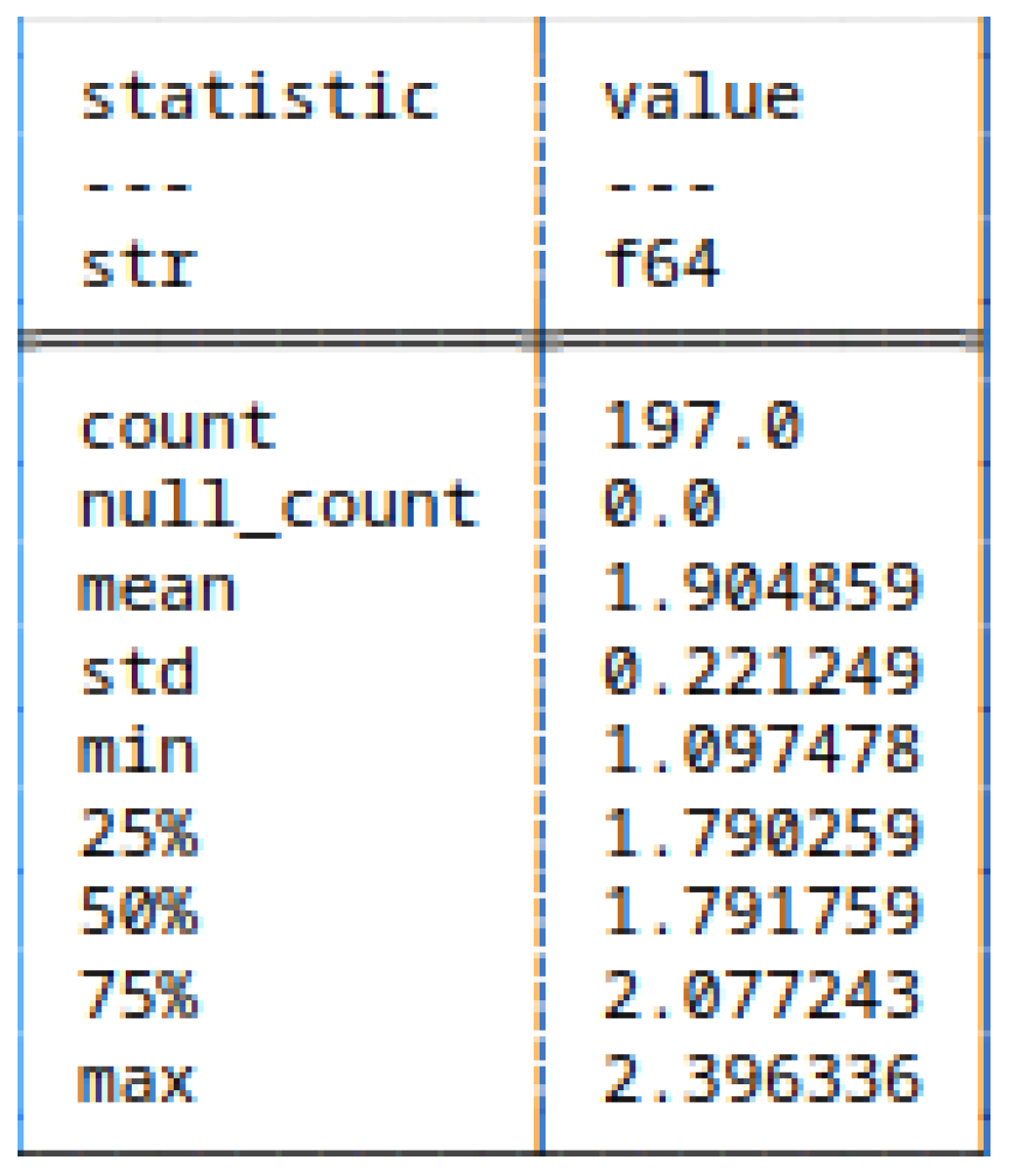
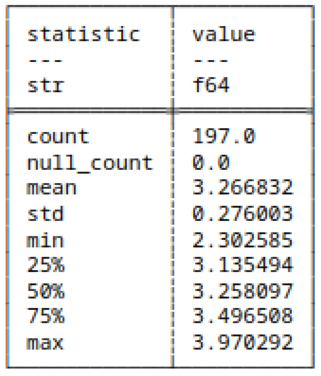
Figure 4.
Descriptive statistics - Shannon Entropy of strings.
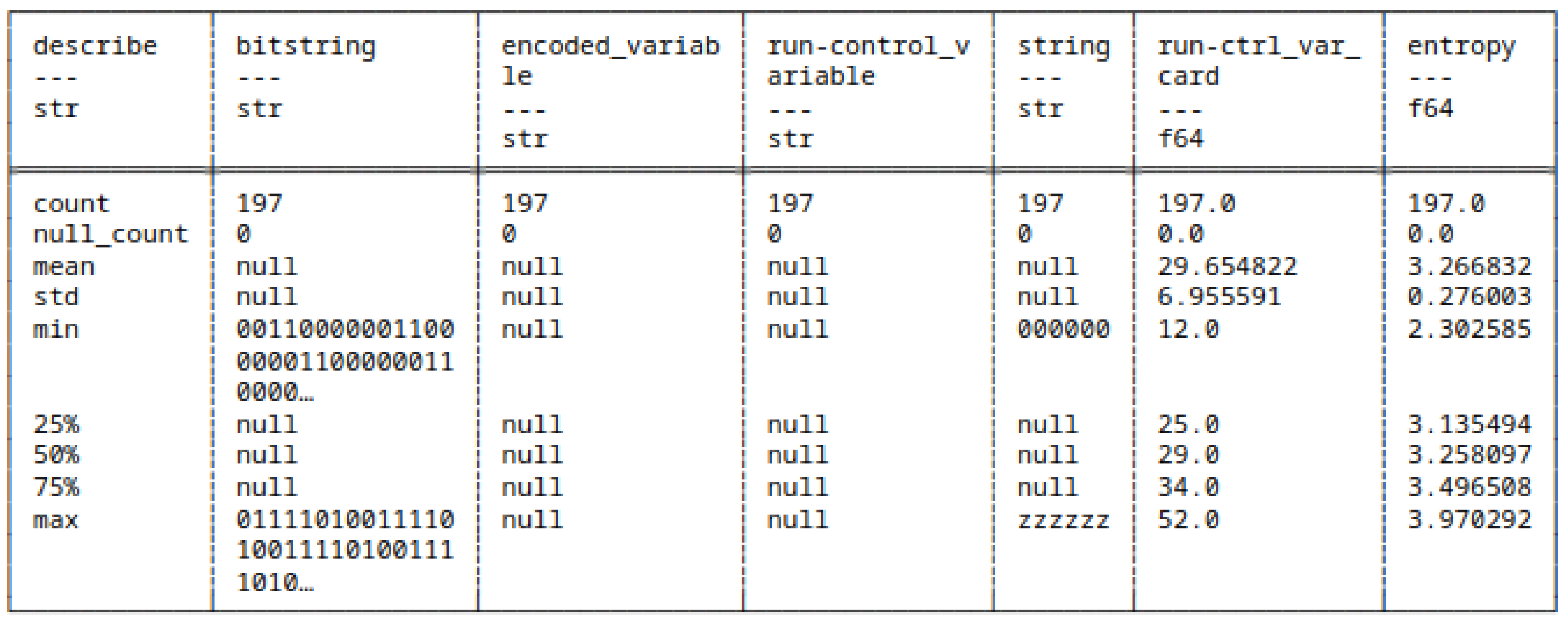
5.3.2. (3) - Run-Length Encoding Applied to Strings
We apply the Run-Length Encoding on the strings.
An excerpt of the Run-Length Encoding applied to the ASCII representation:
([’6’, ’9’, ’6’, ’9’, ’6’, ’9’], [1, 1, 1, 1, 1, 1])
([’L’, ’i’, ’m’, ’a’, ’n’, ’1’, ’0’], [1, 1, 1, 1, 1, 1, 3])
([’a’, ’s’, ’d’, ’f’, ’1’, ’2’, ’3’, ’4’], [1, 1, 1, 1, 1, 1, 1, 1])
([’1’, ’4’, ’7’, ’8’, ’5’, ’2’, ’3’, ’6’, ’9’], [1, 1, 1, 1, 1, 1, 1, 1, 1])
([’a’, ’s’, ’d’, ’1’, ’2’, ’3’], [1, 1, 1, 1, 1, 1])
([’d’, ’a’, ’n’, ’i’, ’e’, ’l’], [1, 1, 1, 1, 1, 1])
([’1’, ’2’, ’3’], [1, 1, 1])
([’5’], [7])
In each tuple, the first list represents the encoded variables, the second list represents the run-control variables.
Note
Run-Length Encoding computed using python-rle (Appendix H).
5.3.3. (4) - Huffman Coding Applied to Strings
In this case, we transform the string representation into its Huffman Coding form. This setting explores how a reduced output alphabet({0,1}) impacts the Shannon Entropy and Algorithmic Complexity.
An excerpt of the Huffman Coding (HC) applied to strings:
696969 010101
Liman1000 001011100010101000111111
asdf1234 100111101110000001010011
147852369 11100011001010101111000011110
asd123 1110100100101110
daniel 1011000111111000
123 10110
5555555 --> The alphabet for Huffman must contain at least two symbols. <--
The first column represents the string and the second column its Huffman Coding.
The last row showcases the requirement for the source alphabet to be composed of at least two symbols.
Note
Huffman Coding computed using sagemath (Appendix H).
5.3.4. (5) - Shannon Entropy Applied to HC
In this case, we compute the Shannon Entropy on the Huffman Coding form of the string.
Some examples include the following:
696969 010101 1.7917063276766527
Liman1000 001011100010101000111111 3.1780011182265513
asdf1234 100111101110000001010011 3.1780006887965433
147852369 11100011001010101111000011110 3.3672433317994823
asd123 1110100100101110 2.772536500777123
daniel 1011000111111000 2.772536500777123
123 10110 1.6093870364705087
The first column represents the initial string, the second column its Huffman Coding and the third column represents the entropy of its HC form.
Figure 5.
Histogram: Shannon Entropy - HC form.
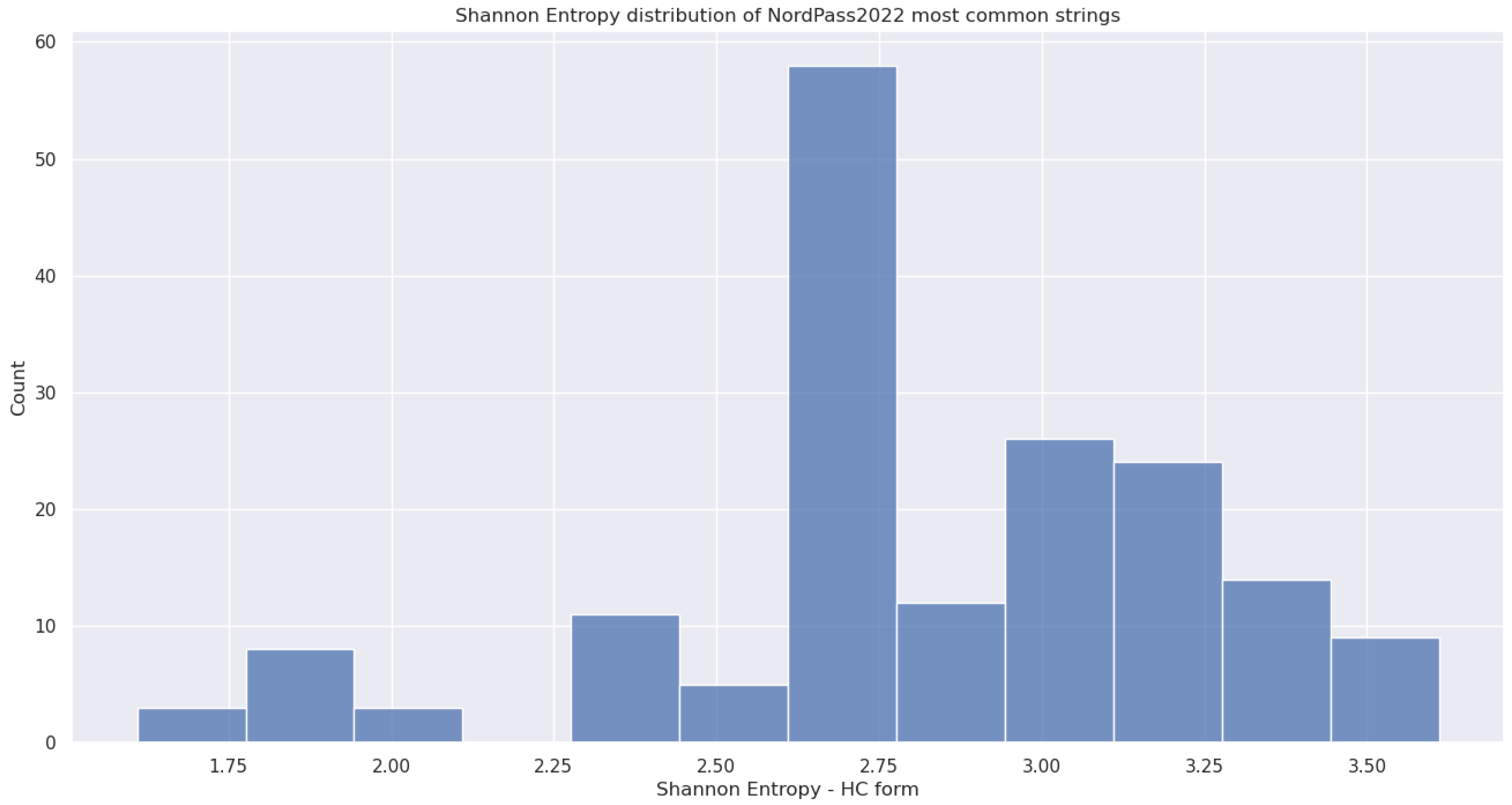
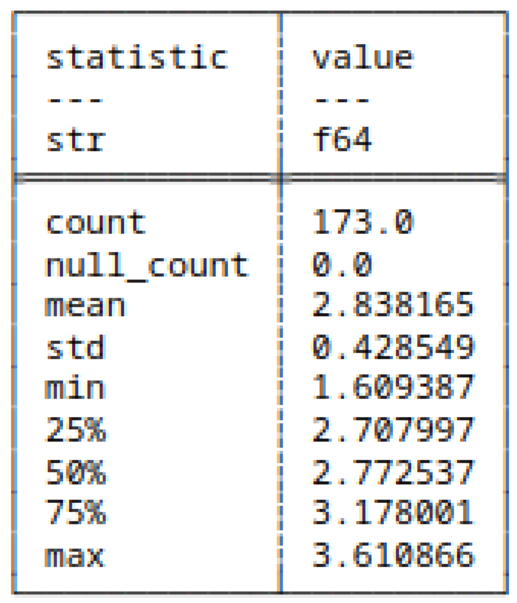
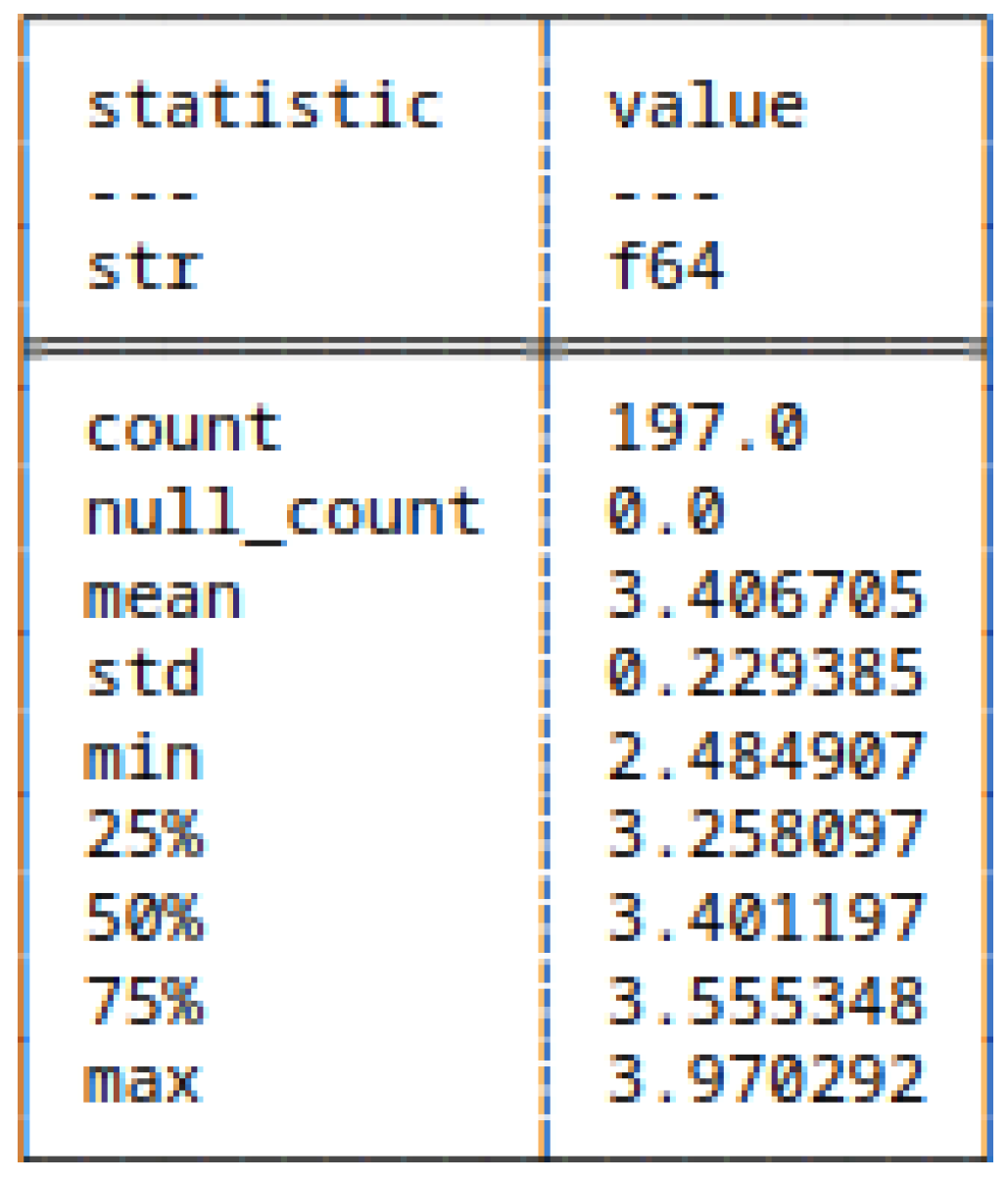
Figure 6.
Descriptive statistics - Entropy of HC.
5.3.5. (6) - Block Decomposition Method Applied to HC
In this section, we look at the Block Decomposition Method compute of the Huffman Coding form of strings.
Hereafter, follows some examples:
Liman1000 001011100010101000111111 65.28075296319241
asdf1234 100111101110000001010011 66.64156258471269
147852369 11100011001010101111000011110 68.67718649444342
asd123 1110100100101110 32.835380112641985
daniel 1011000111111000 32.58846537217148
The first column represents the initial string, the second column its Huffman Coding and the third column represents the Algorithmic Complexity approximation using Block Decomposition Method of its HC form.
We note that the minimum length required to be able to compute is twelve, which brings the number of computed elements to 148.
Figure 7.
Histogram: Algorithmic Complexity - strings HC form.
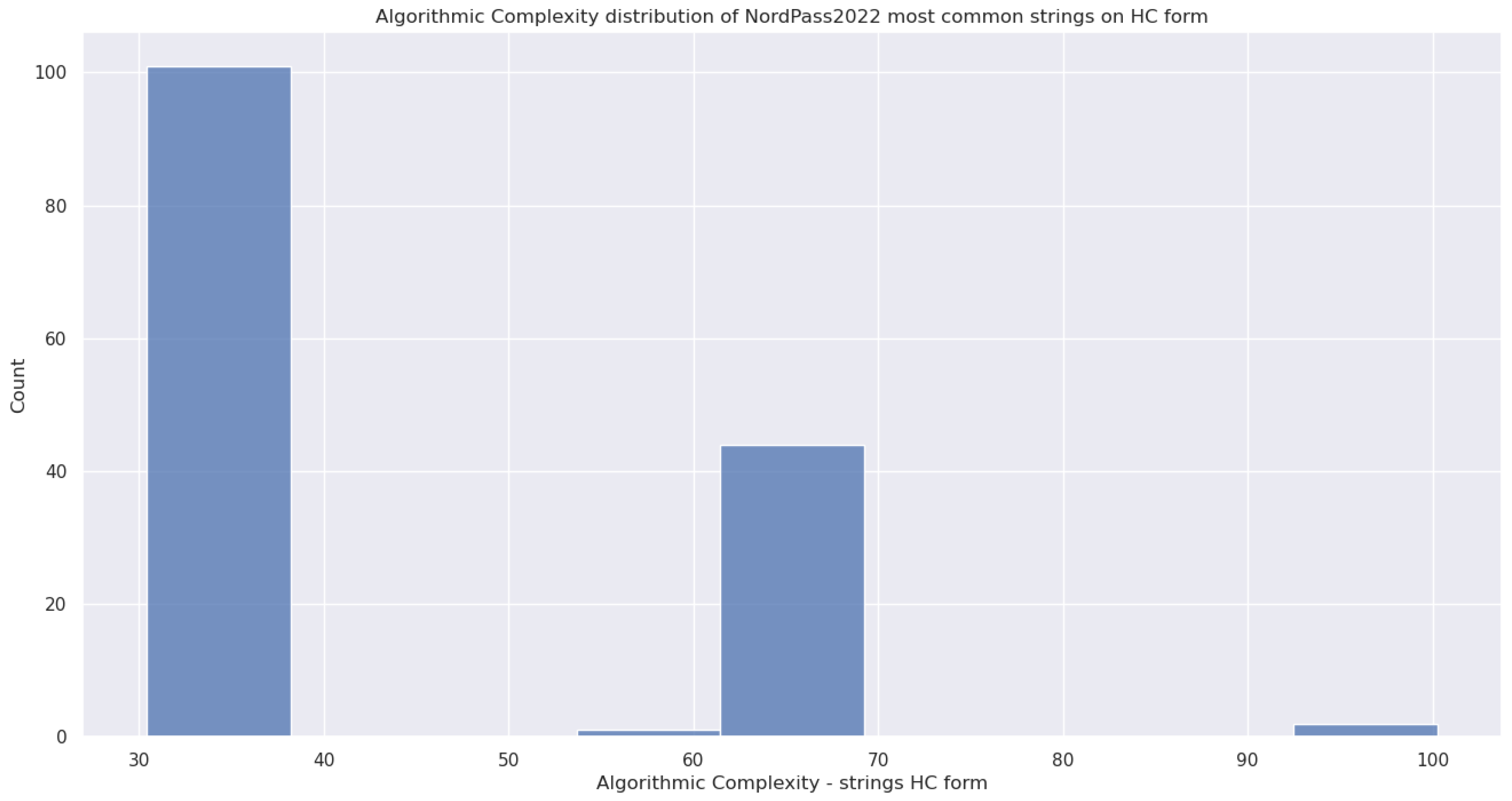
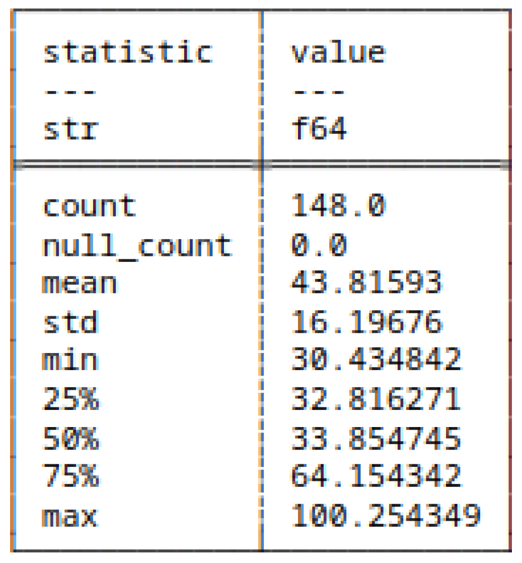
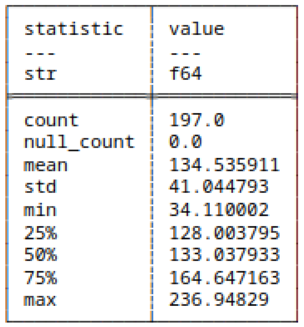
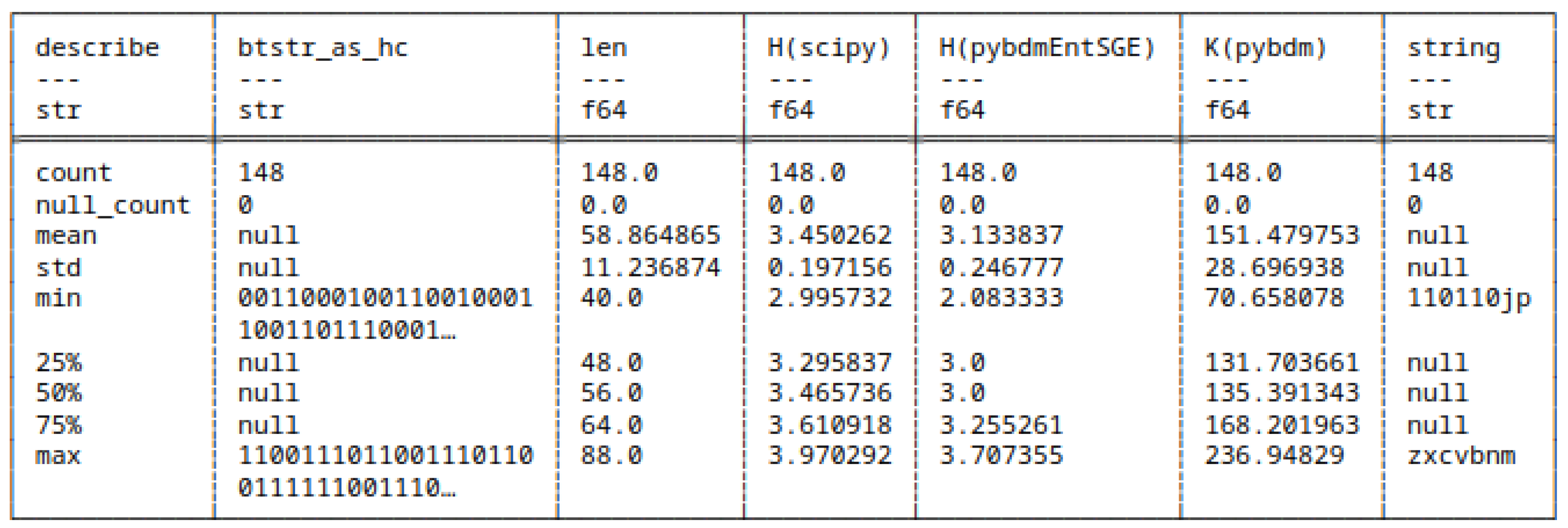
Figure 8.
Descriptive statistics - BDM of HC.
5.4. Strings as Bitstrings
In this section, if applicable, we consider the previously applied computations on the bitstring representation of the strings.
By bitstring, we mean the binary representation(output alphabet consisting of {0,1} only) of a string e.g.:
(abcd): 01100001011000100110001101100100
5.4.1. (7) - Shannon Entropy of Bitstrings
We start by computing the Shannon Entropy of the binary representation of the string.
An excerpt of the computed values:
696969
(’001101100011100100110110001110010011011000111001’, 3.1780538303479453)
Liman1000
(’010011000110100101101101011000010110111000110001001100000011000000110000’, 3.367295829986474)
asdf1234
(’0110000101110011011001000110011000110001001100100011001100110100’, 3.3322045101752034)
147852369
(’001100010011010000110111001110000011010100110010001100110011011000111001’, 3.4965075614664802)
asd123
(’011000010111001101100100001100010011001000110011’, 3.0445224377234235)
Figure 9.
Histogram: Shannon Entropy - bitstrings (scipy).
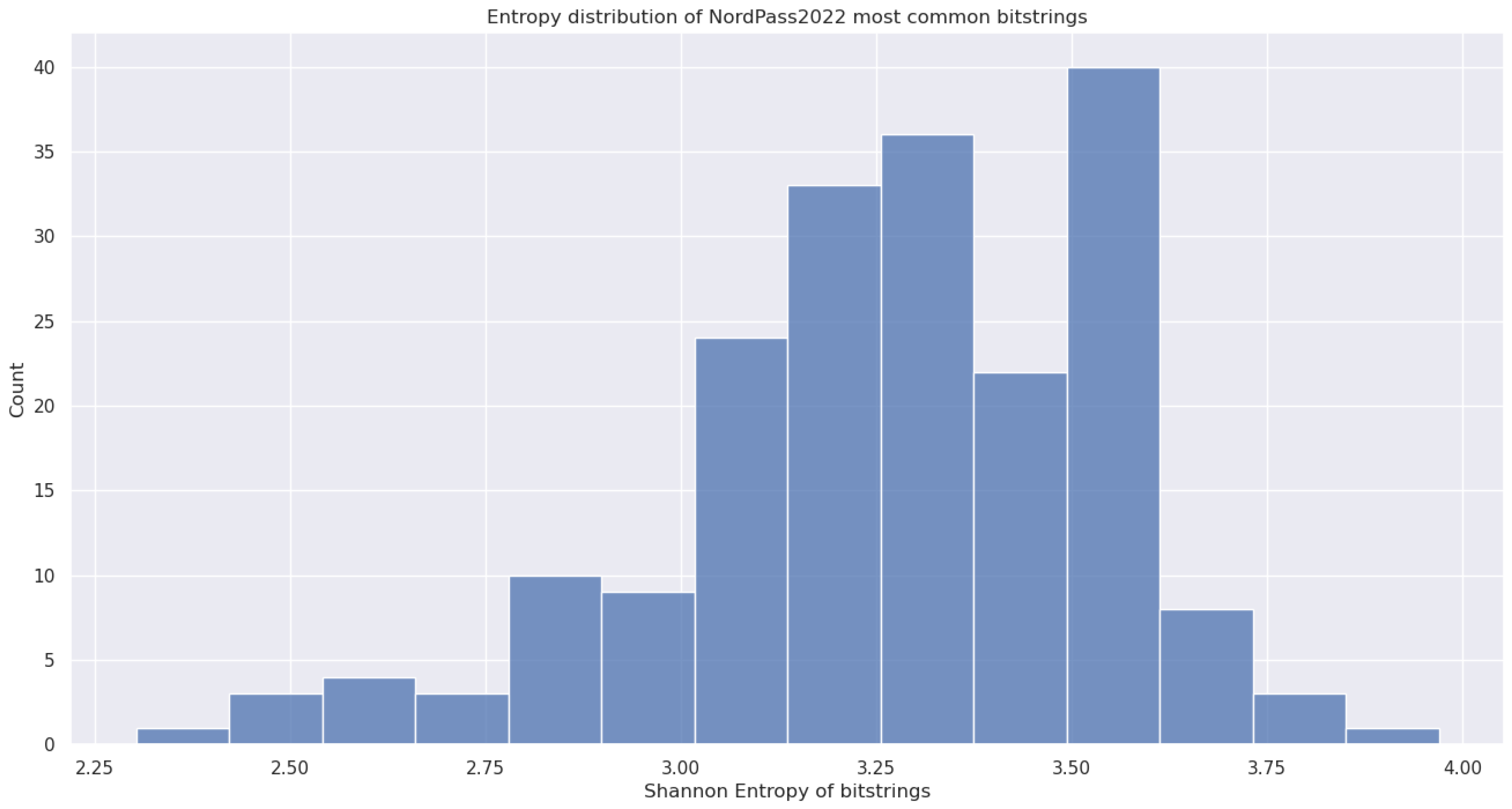
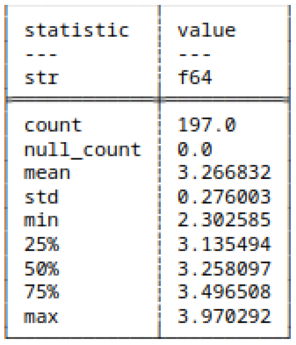
Figure 10.
Descriptive statistics - H of bitstrings.
5.4.2. (8) - Block Decomposition Method Applied to Bitstrings
In this case, we compute the Block Decomposition Method values of the bitstring representation of passwords.
Here are a few examples of values:
696969
(’001101100011100100110110001110010011011000111001’, 135.00537752642254)
Liman1000
(’010011000110100101101101011000010110111000110001001100000011000000110000’, 196.59170185783432)
asdf1234
(’0110000101110011011001000110011000110001001100100011001100110100’, 165.65408264230527)
147852369
(’001100010011010000110111001110000011010100110010001100110011011000111001’, 202.74909242058078)
asd123
(’011000010111001101100100001100010011001000110011’, 135.44662527488683)
Figure 11.
Histogram: Algorithmic Complexity - bitstrings.
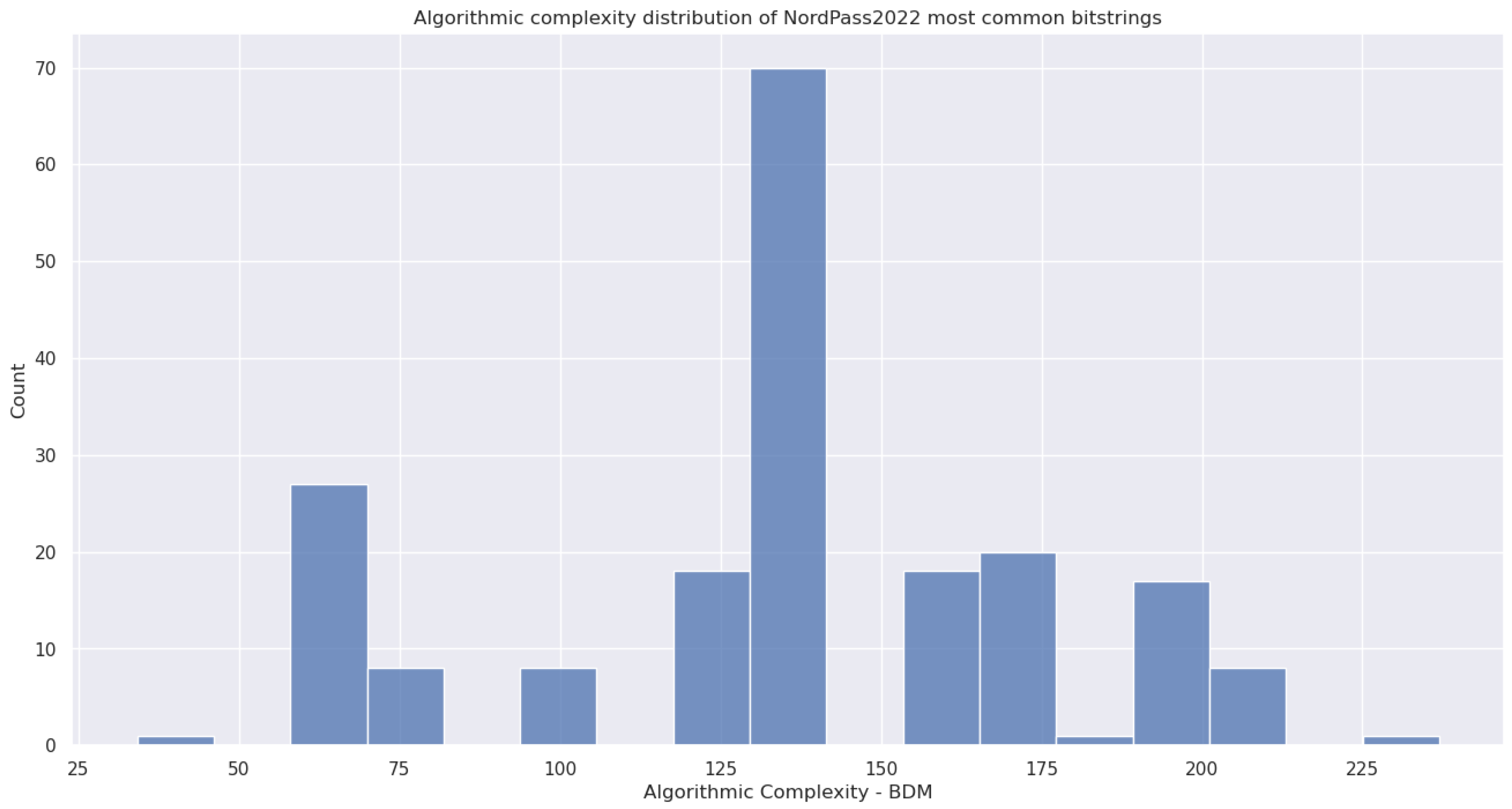
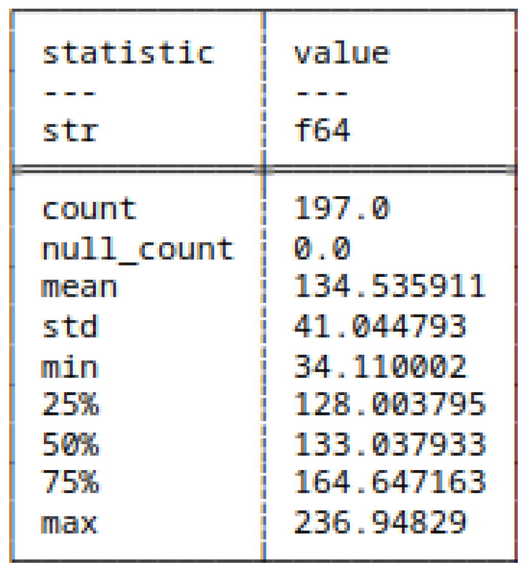
Figure 12.
Descriptive statistics - BDM of bitstrings.
5.4.3. (9) - Run-Length Encoding Applied to Bitstrings
In this section, we apply the Run-Length Encoding on the bitstring representation of passwords.
Because of the huge verbosity, we give one example of the Run-Length Encoding on a bitstring.
The following bistring: 001101100011100100110110001110010011011000111001 representing 696969 is encoded as follows:
[0, 1, 0, 1, 0, 1, 0, 1, 0, 1, 0, 1, 0, 1, 0, 1, 0, 1, 0, 1, 0, 1, 0, 1]
[2, 2, 1, 2, 3, 3, 2, 1, 2, 2, 1, 2, 3, 3, 2, 1, 2, 2, 1, 2, 3, 3, 2, 1]
The first list represents the encoded variable. The second list represents the run-control variable. In order to reconstruct the original bitstring, one has to take the symbol of the first list and have its occurrence multiplied by the integer in the run-control variable list. This process has to be repeated for each encoded variable. In the end, their concatenations yield back the original bitstring.
For readability sake, we have removed the single quotes from the symbols of the encoded variable list.
5.4.4. (10) - Huffman Coding Applied to Bitstrings
In this case, we take the Huffman Coding representation of a bitstring.
Here are some computed encodings:
696969
001101100011100100110110001110010011011000111001
001101100011100100110110001110010011011000111001
Liman1000
010011000110100101101101011000010110111000110001001100000011000000110000
101100111001011010010010100111101001000111001110110011111100111111001111
asdf1234
0110000101110011011001000110011000110001001100100011001100110100
1001111010001100100110111001100111001110110011011100110011001011
147852369
001100010011010000110111001110000011010100110010001100110011011000111001
110011101100101111001000110001111100101011001101110011001100100111000110
asd123
011000010111001101100100001100010011001000110011
100111101000110010011011110011101100110111001100
daniel
011001000110000101101110011010010110010101101100
100110111001111010010001100101101001101010010011
123
001100010011001000110011
110011101100110111001100
For each group of three lines, the first line represents the initial string, the second line its binary form and the third its Huffman Coding representation.
We notice that applying the Huffman Coding to the bitstring representation generate two possible outcome. One output behaves like the bitwise AND operator results to zero. The other case acts as the identity operator.
5.4.5. (11) - Shannon Entropy Applied to HC
For this case, we compute the Shannon Entropy of the Huffman Coding form of bitstrings.
Here follows a few computed values:
696969
001101100011100100110110001110010011011000111001 3.1780538303479453
Liman1000
101100111001011010010010100111101001000111001110110011111100111111001111 3.761200115693562
asdf1234
1001111010001100100110111001100111001110110011011100110011001011 3.58351893845611
147852369
110011101100101111001000110001111100101011001101110011001100100111000110 3.6635616461296463
asd123
100111101000110010011011110011101100110111001100 3.295836866004329
For every pair of lines, the first line is the initial string, the second represents its Huffman Coding followed by its Shannon Entropy.
Figure 13.
Histogram: Shannon Entropy - bitstrings HC form.
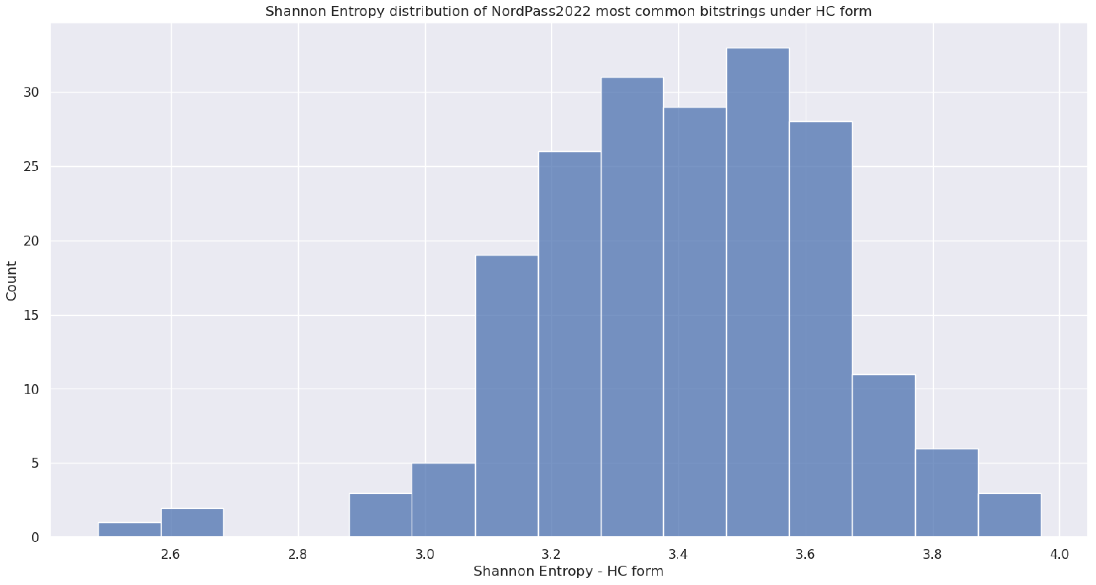
Figure 14.
Descriptive statistics - Shannon Entropy of bitstrings HC form.
5.4.6. (12) - Block Decomposition Method Applied to HC
In this section, we compute the Algorithmic Complexity approximation using the Block Decomposition Method of the Huffman Coding of the bitstrings.
Here is an excerpt of the computed values:
696969
001101100011100100110110001110010011011000111001 135.00537752642254
Liman1000
101100111001011010010010100111101001000111001110110011111100111111001111 196.59170185783432
asdf1234
1001111010001100100110111001100111001110110011011100110011001011 165.65408264230527
147852369
110011101100101111001000110001111100101011001101110011001100100111000110 202.74909242058078
asd123
100111101000110010011011110011101100110111001100 135.44662527488683
For every pair of lines, the first line is the initial string, the second represents its Huffman Coding followed by its approximated Algorithmic Complexity value.
Figure 15.
Histogram: Algorithmic Complexity - bitstrings HC form.

Figure 16.
Descriptive statistics - BDM of bitstrings HC form.
5.5. Shannon Entropy of Strings and Bitstrings - t-Test
In this section, we look at how an object in a given alphabet(source) influences its Shannon Entropy. Remark, if not explicitly stated, the H is computed using the scipy library.
We consider a t-test, the entropies of strings constitute the first sample and, the entropies of bitstrings constitute the second sample.
Figure 17.
Descriptive statistics - H of strings.
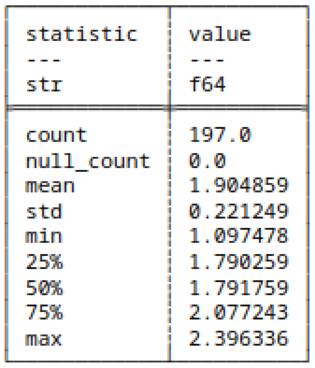
Figure 18.
Descriptive statistics - H of bitstrings.
We use a t-test to quantify the statistical difference between the two samples.
We report a t-test of:
Thus, we can say that the mean entropy of the strings are significantly lower than the mean of their bitstring counterpart.
5.6. Run-Length Encoding of Strings and Bitstrings
Figure 19.
RLE of 10 lowest entropy strings.
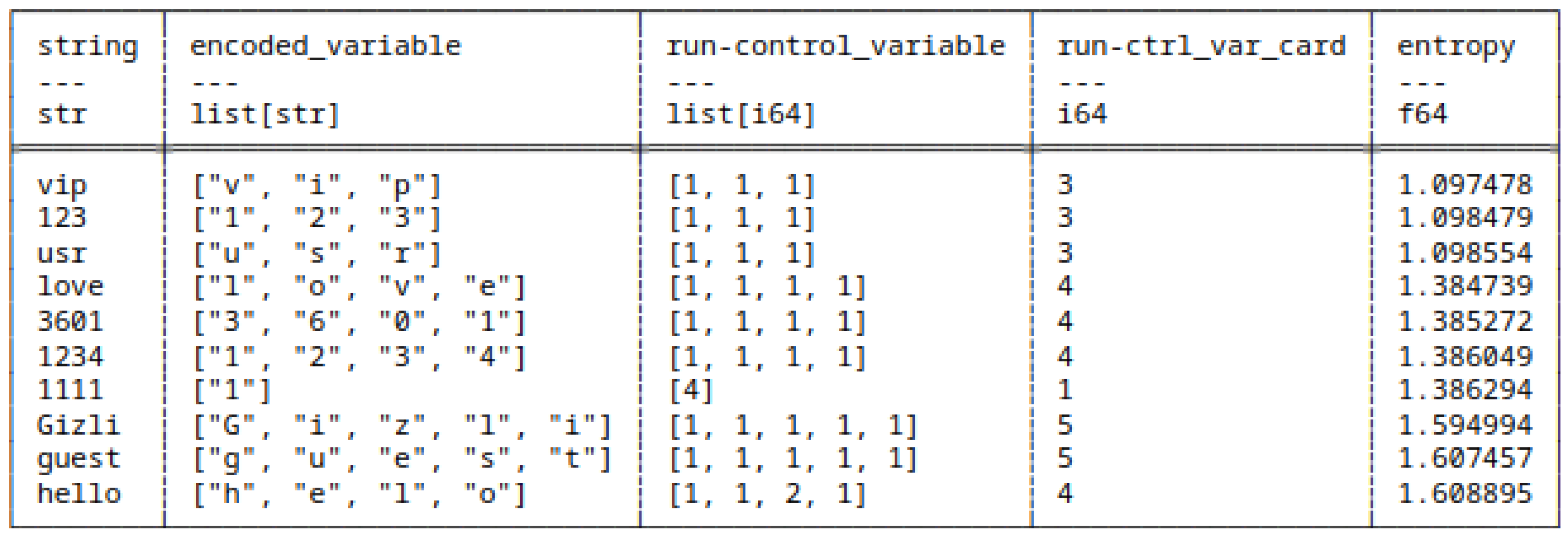
Figure 20.
RLE of 10 highest entropy strings.
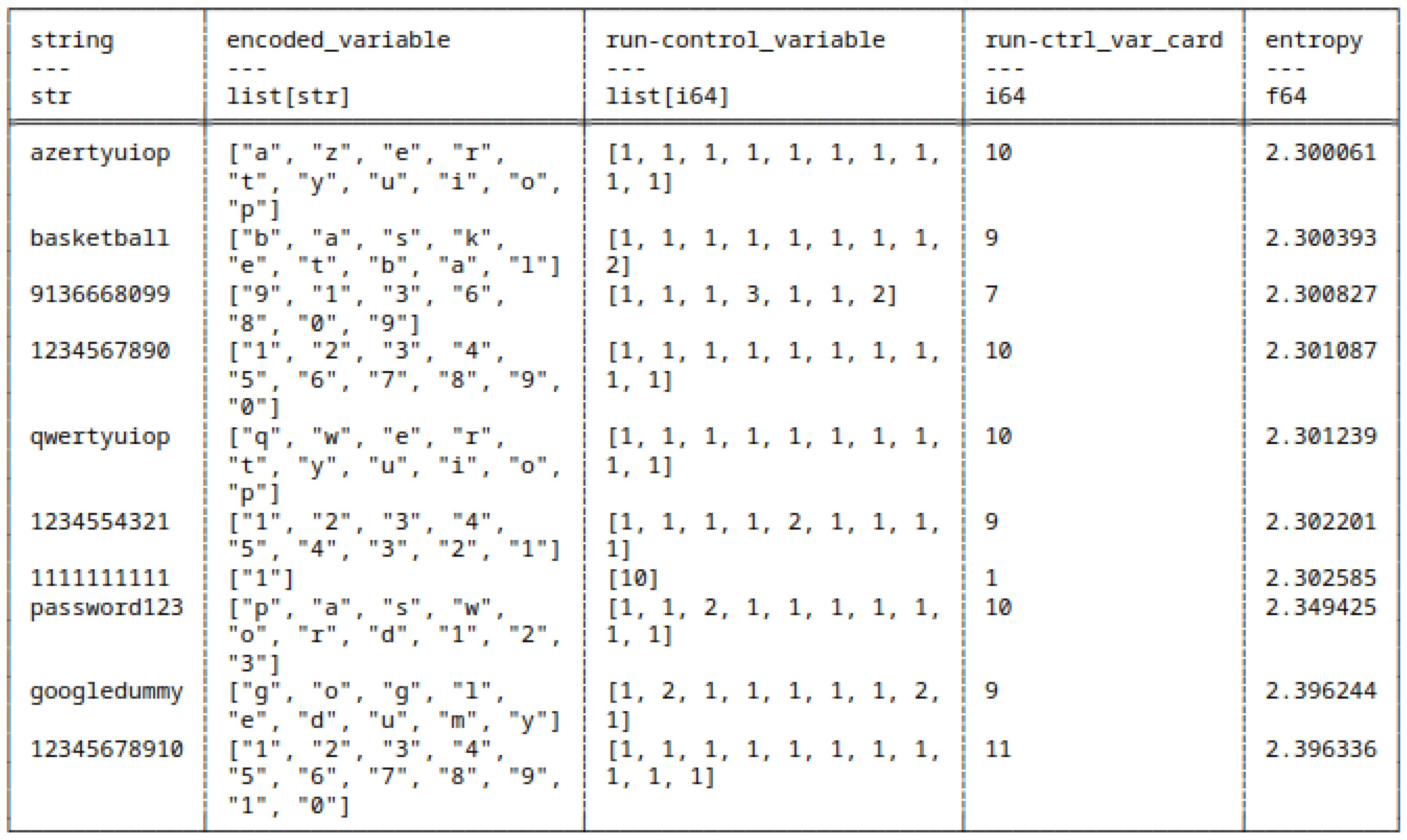
Figure 21.
RLE of 10 lowest entropy bitstrings - 1.
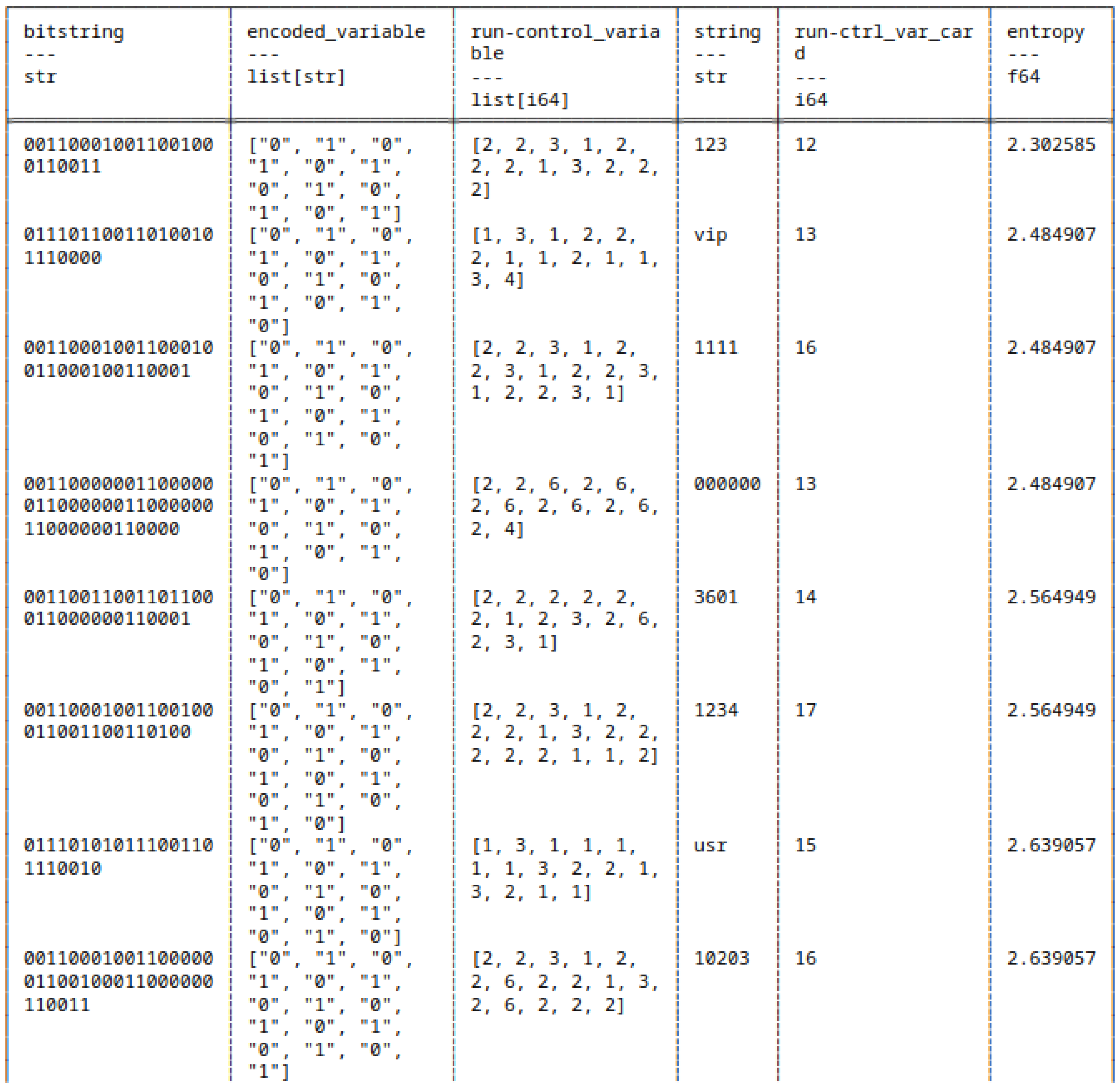
Figure 22.
RLE of 10 lowest entropy bitstrings - 2.
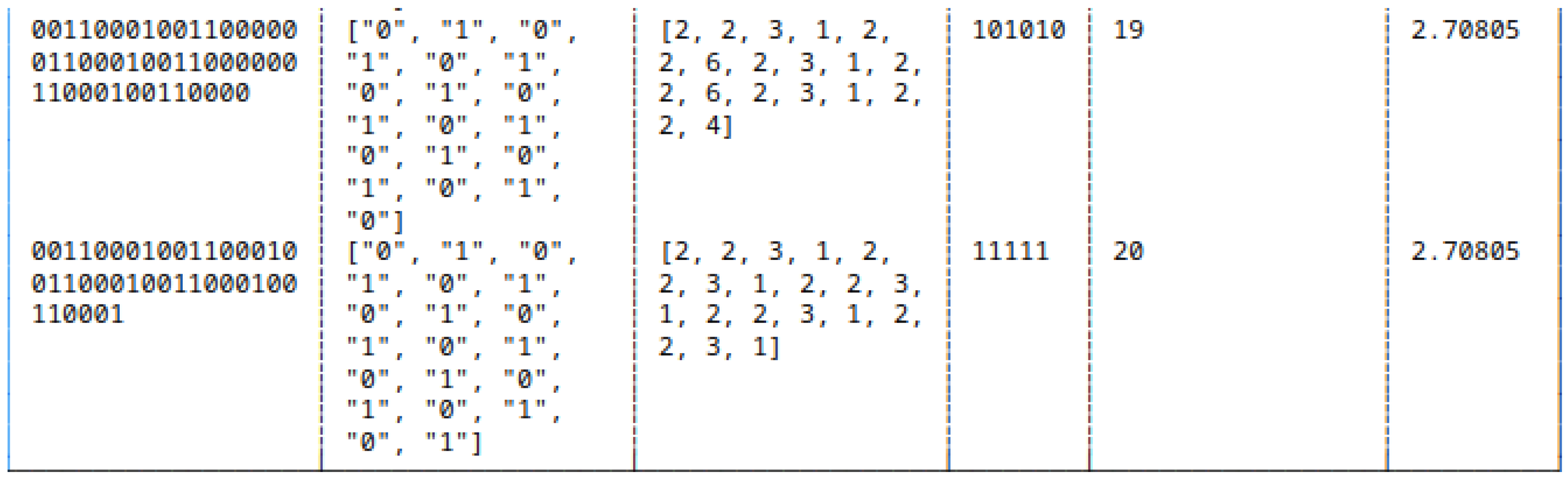
Figure 23.
RLE of 10 highest entropy bitstrings - 1.
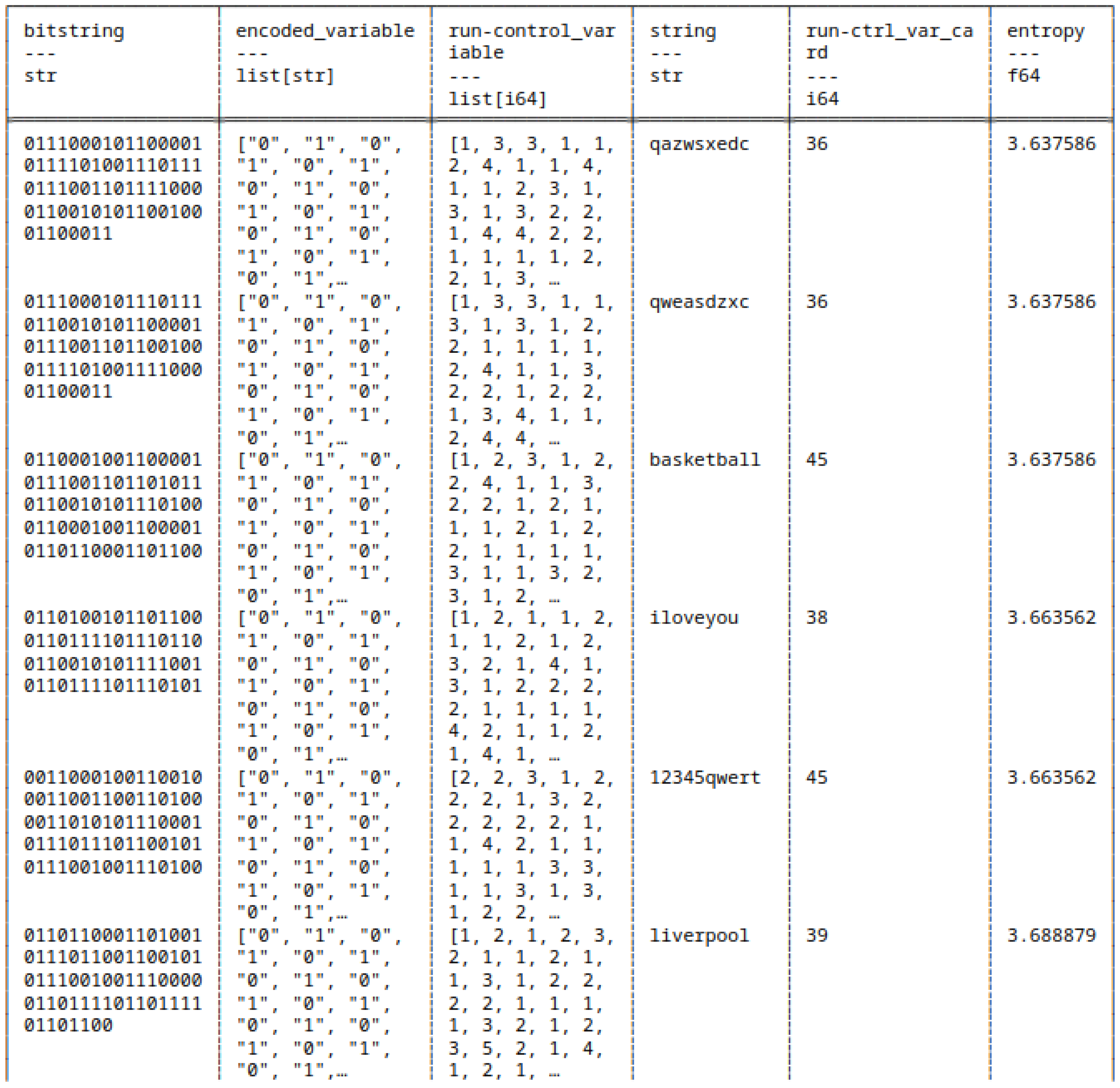
Figure 24.
RLE of 10 highest entropy bitstrings - 2.
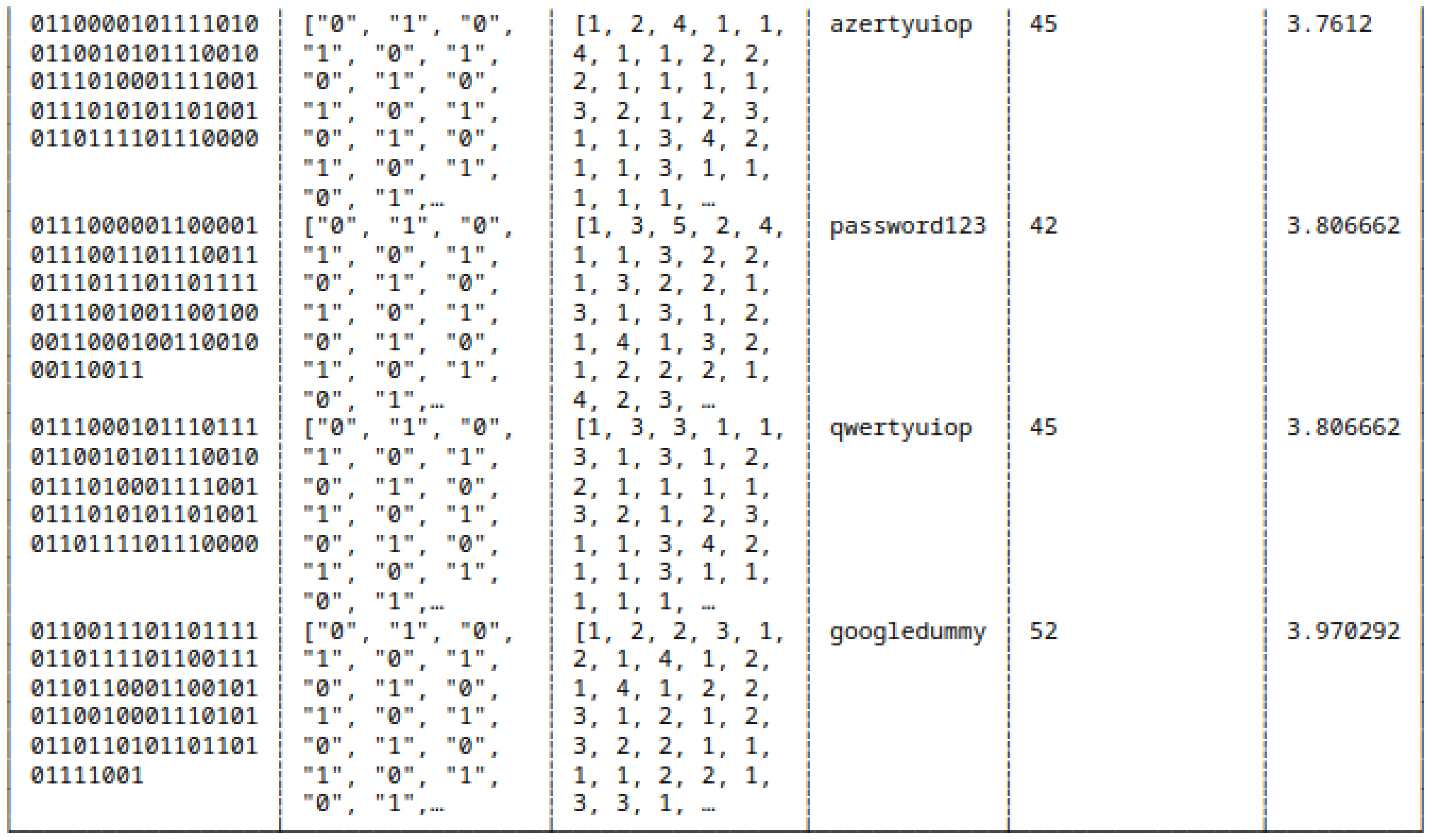
Figure 25.
Descriptive statistics - strings H and corresponding RLE.
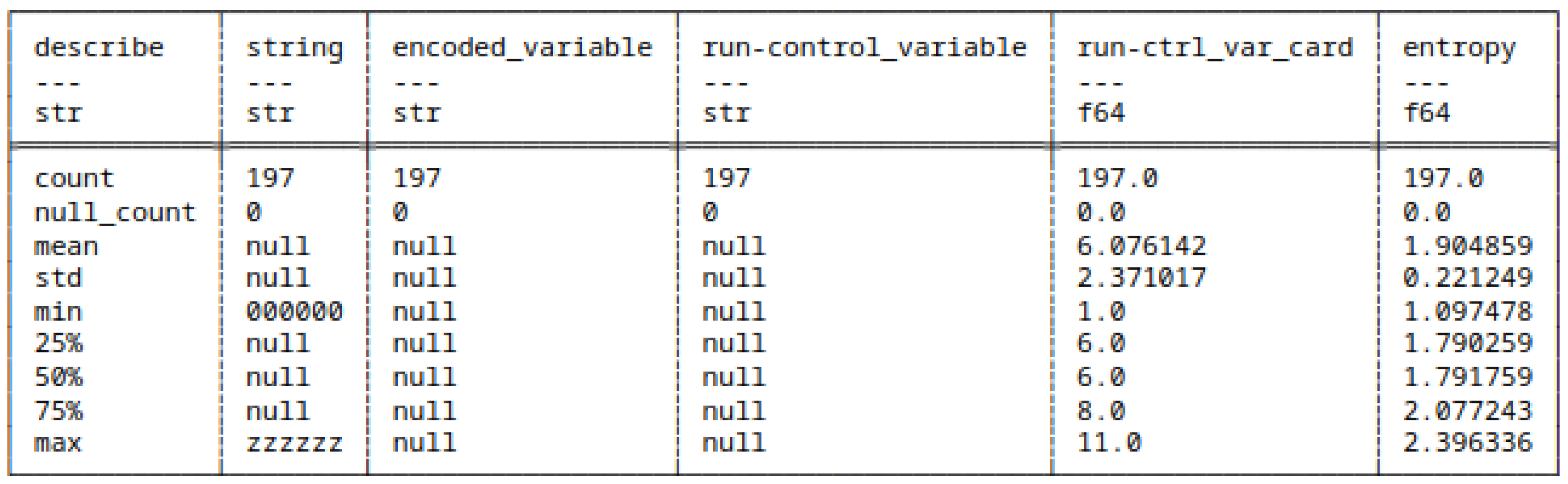
Figure 26.
Descriptive statistics - bitstrings H and corresponding RLE.
5.7. Huffman Coding of Strings and Bitstrings
In this section, we compare various combinations of computed entropies and Algorithmic Complexity (AC). Specifically, we extract based on Shannon Entropy (H) and Algorithmic Complexity the 10 lowest and 10 highest strings and bitstrings under their Huffman Coding form.
5.7.1. Huffman Encoded Strings
In the following, we look at the Huffman Coding representation of strings. We compute their entropies under the software packages of:
- scipy,
- pybdmEnt - default entropy implementation of pybdm package,
- pybdmEntSGE - our entropy implementation using the Schürmann-Grassberger estimator, see eq. (7),
- Their approximated Algorithmic Complexity (AC) or K using the Block Decomposition Method with pybdm.
Figure 27.
10 strings with lowest H in their HC form - sorted(asc.) on H(scipy).
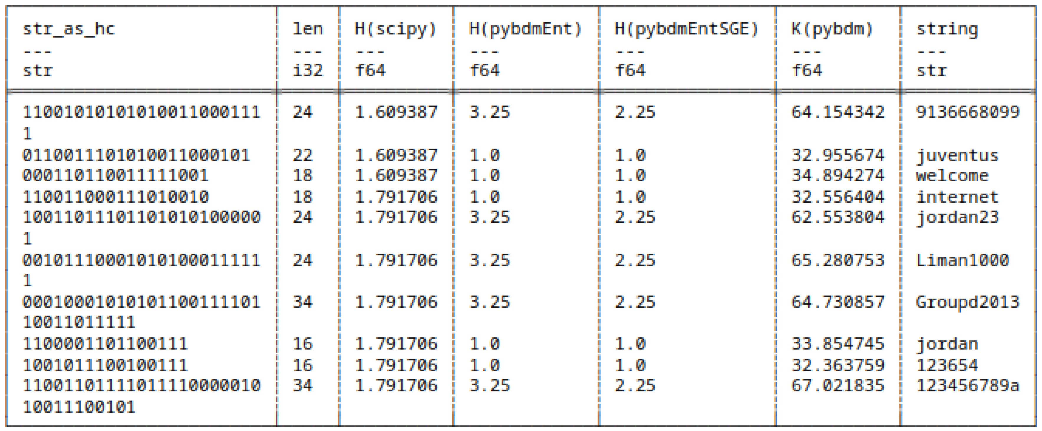
Figure 28.
10 strings with highest H in their HC form - sorted(asc.) on H(scipy).
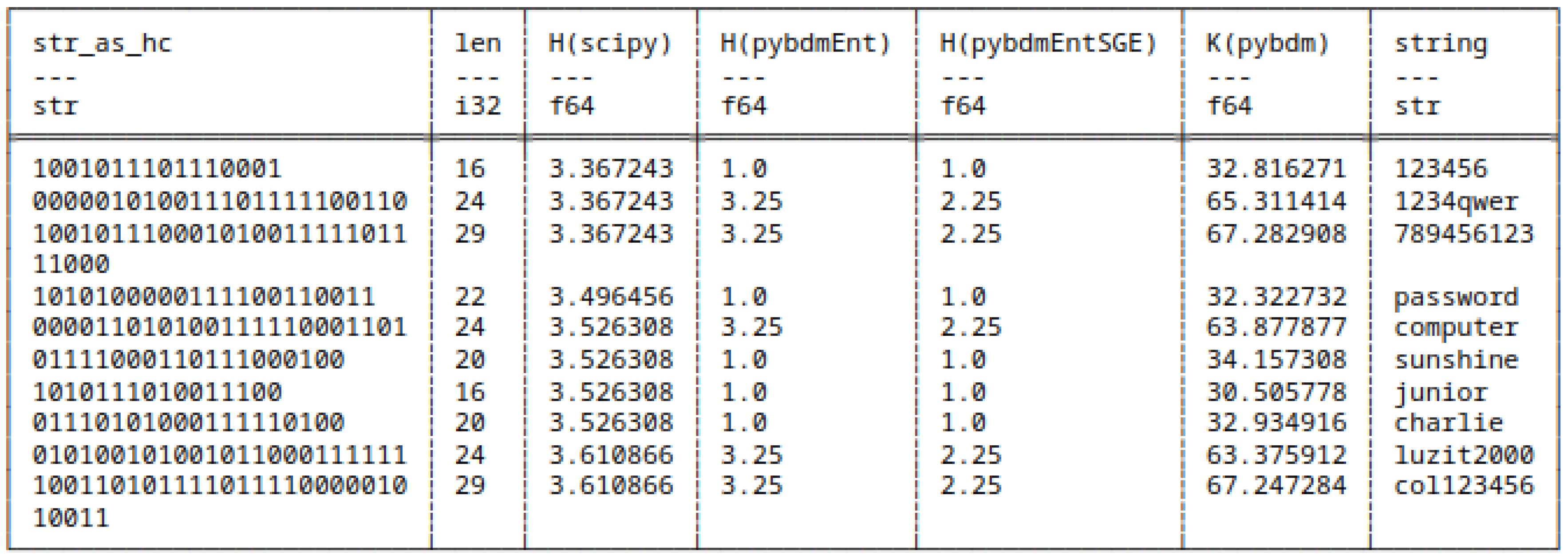
Figure 29.
10 strings with lowest H in their HC form - sorted(asc.) on H(pybdmEnt).
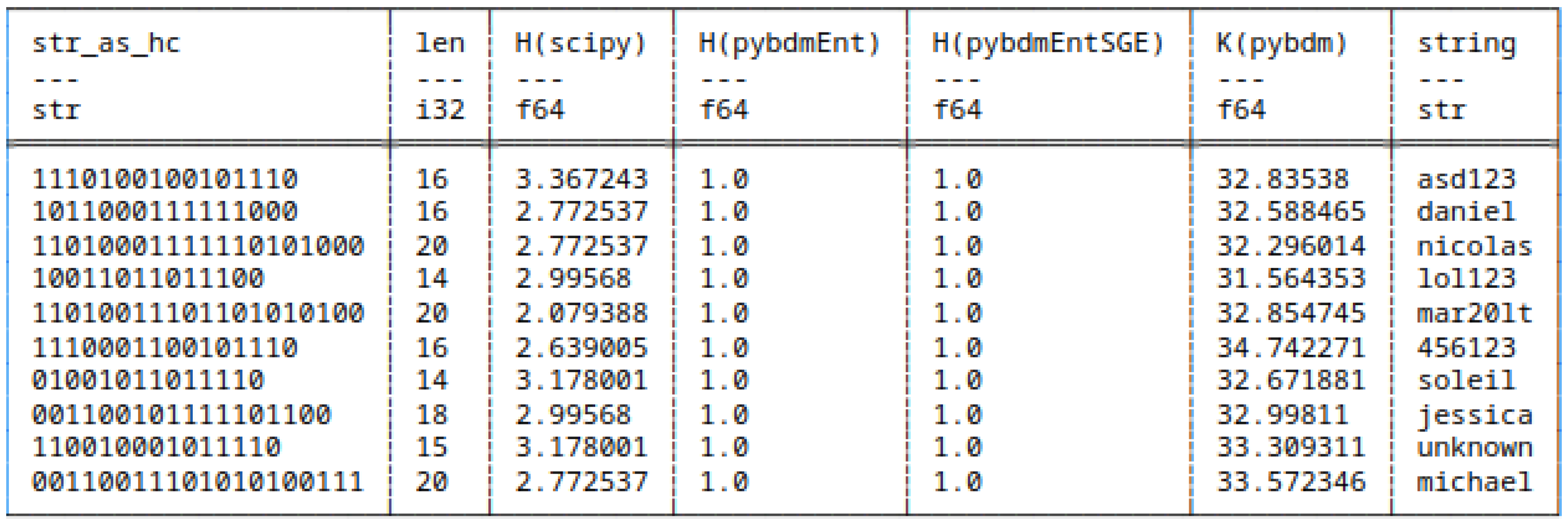
Figure 30.
10 strings with highest H in their HC form - sorted(asc.) on H(pybdmEnt).
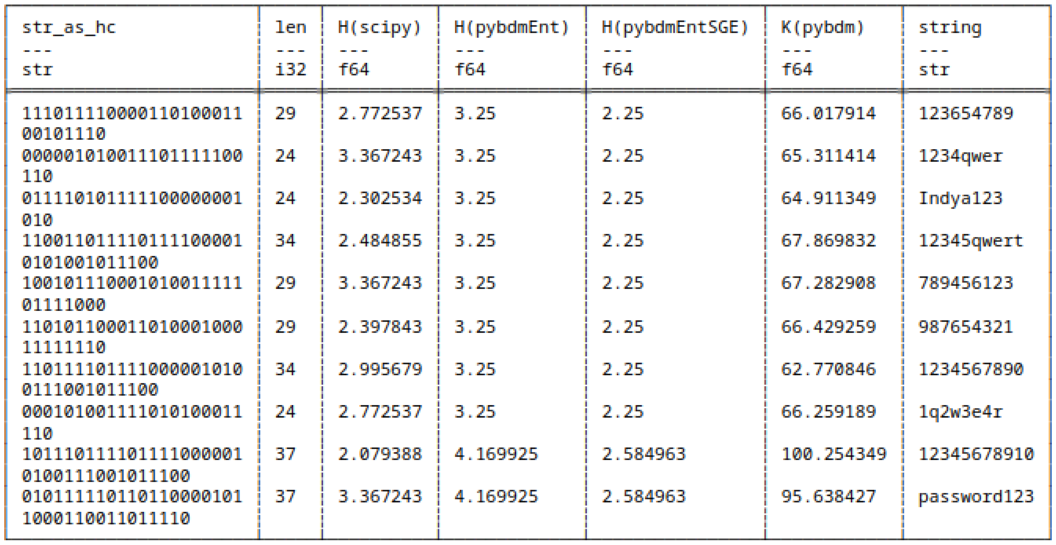
Figure 31.
10 strings with lowest H in their HC form - sorted(asc.) on H(pybdmEntSGE).
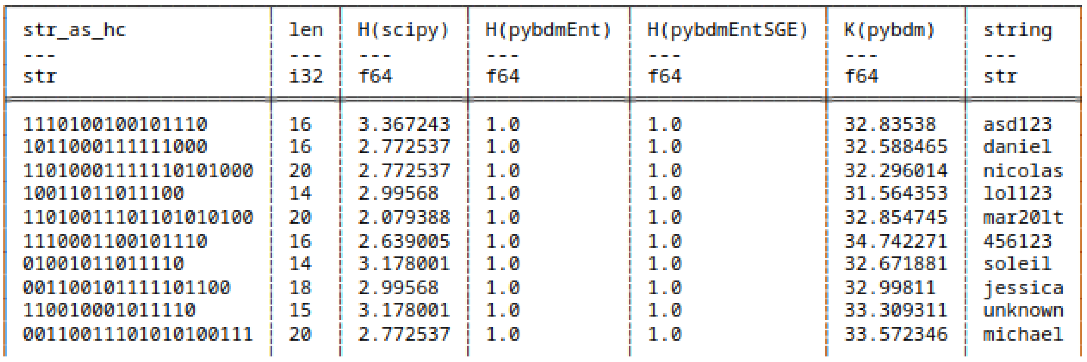
Figure 32.
10 strings with highest H in their HC form - sorted(asc.) on H(pybdmEntSGE).
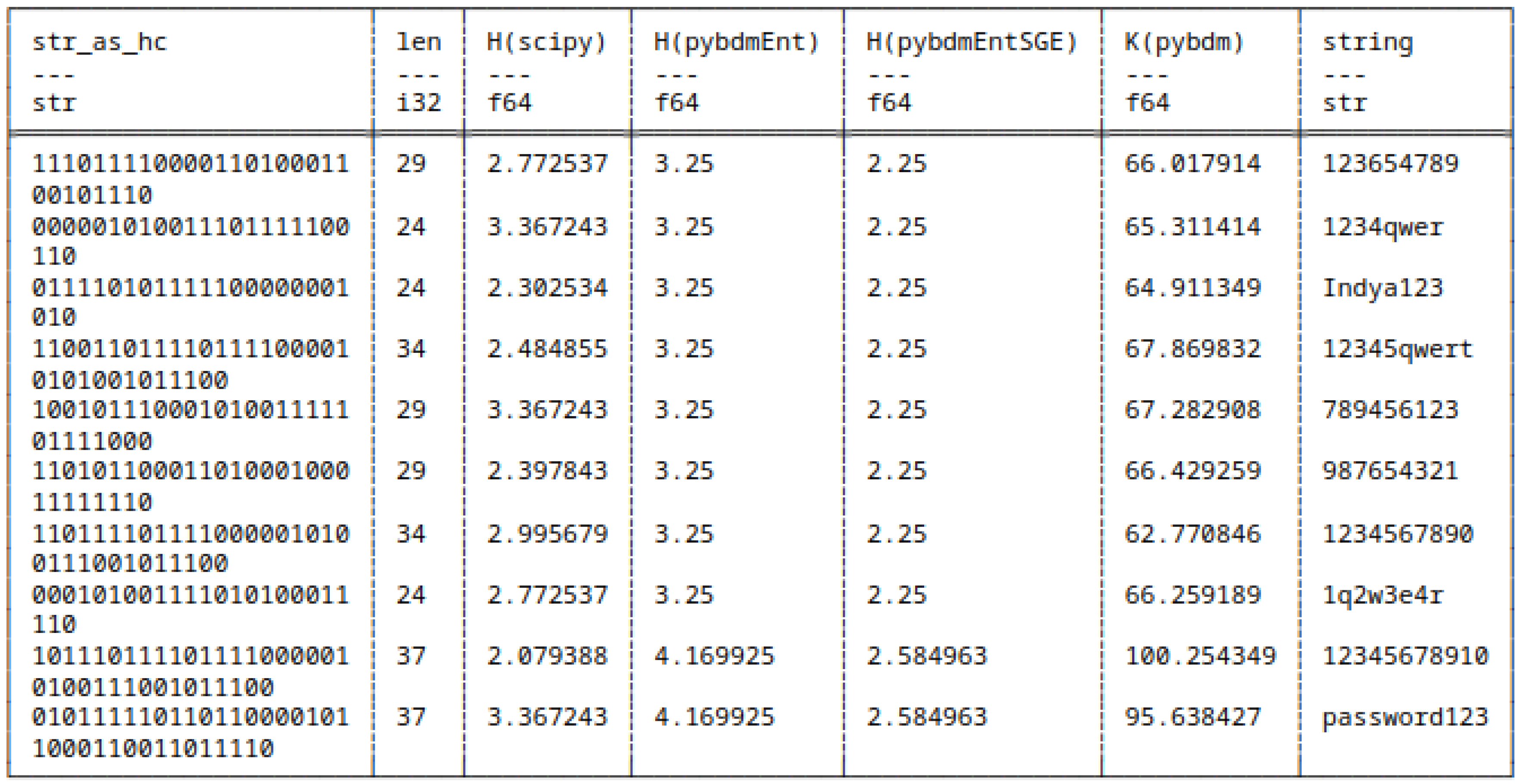
Figure 33.
10 strings with lowest K in their HC form - sorted(asc.) on approximated K(algorithmic complexity).
Figure 33.
10 strings with lowest K in their HC form - sorted(asc.) on approximated K(algorithmic complexity).
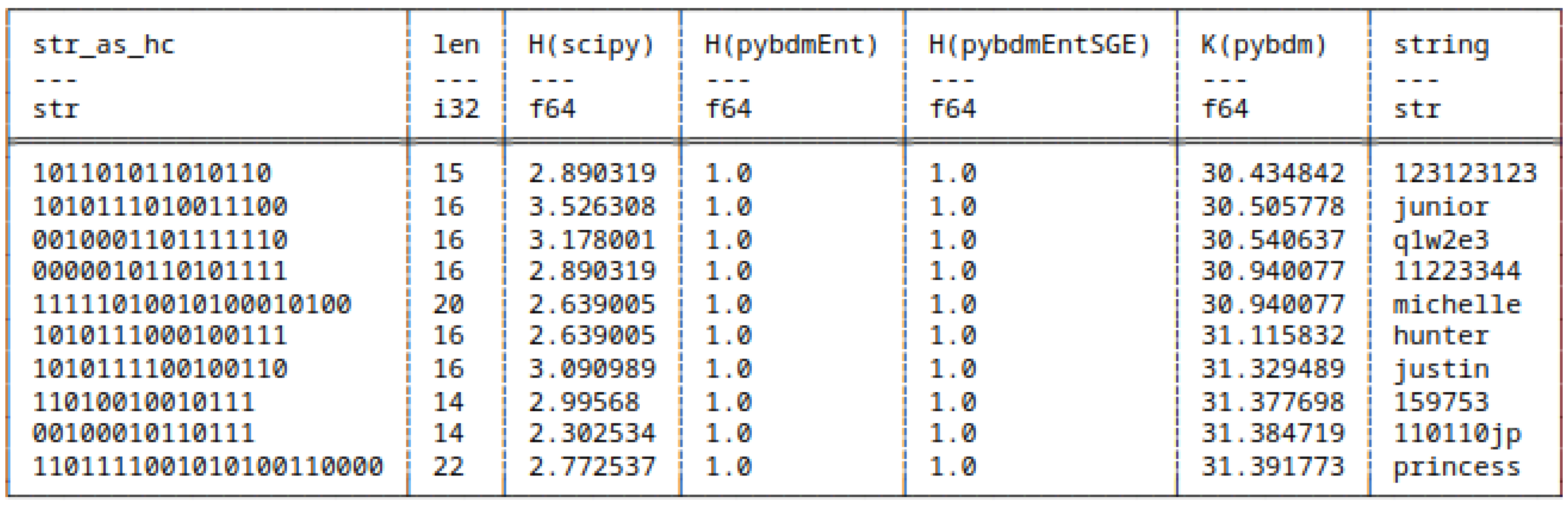
Figure 34.
10 strings with highest K in their HC form - sorted(asc.) on approximated K(algorithmic complexity).
Figure 34.
10 strings with highest K in their HC form - sorted(asc.) on approximated K(algorithmic complexity).
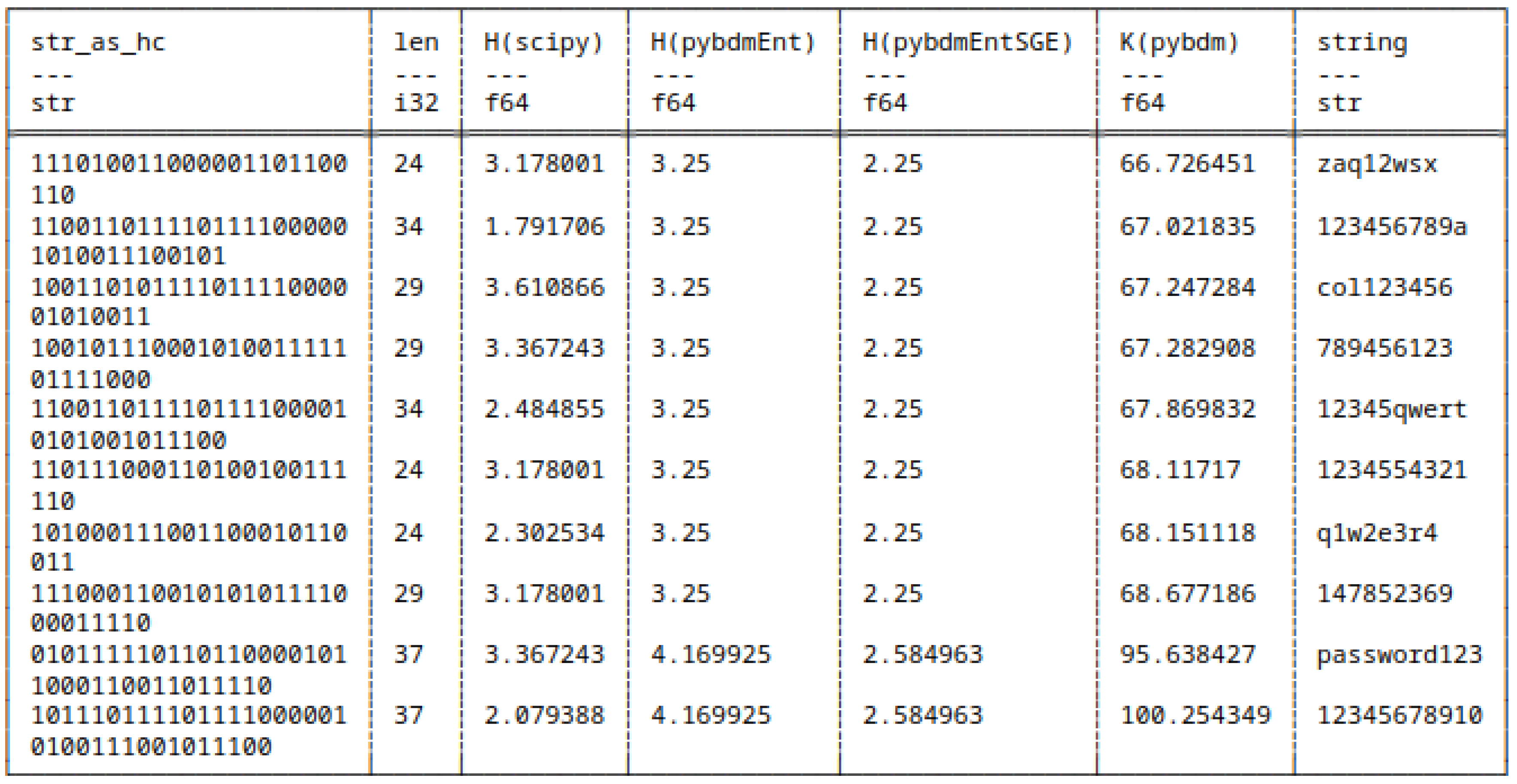
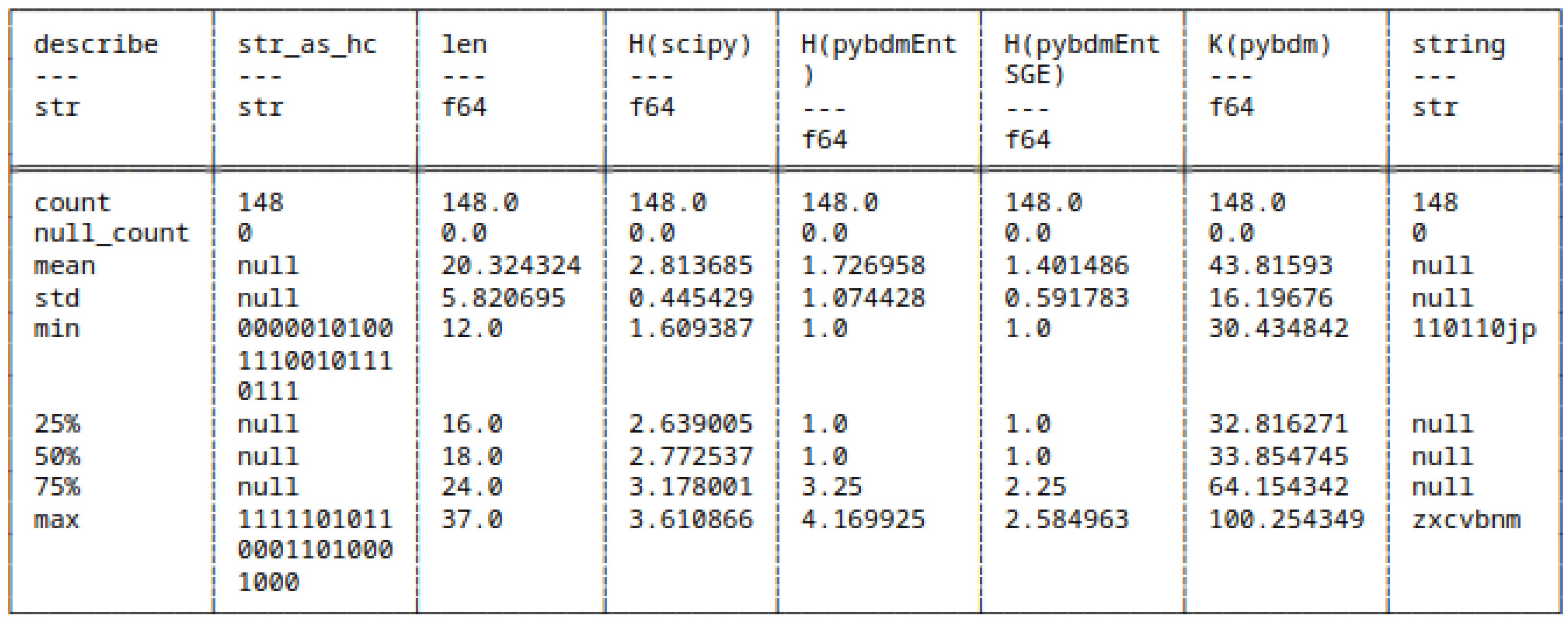
Figure 35.
Descriptive statistics - strings in their HC form.
5.7.2. Huffman Encoded Bitstrings
In the following, we analyse the Huffman Coding representation of bitstrings. We compute their entropies under the software packages of:
- scipy,
- pybdmEntSGE - our entropy implementation using the Schürmann-Grassberger estimator, see eq. (7),
- Their approximated Algorithmic Complexity (AC) or K using the Block Decomposition Method with pybdm.
Figure 36.
10 bitstrings with lowest H in their HC form - sorted(asc.) on H(scipy).
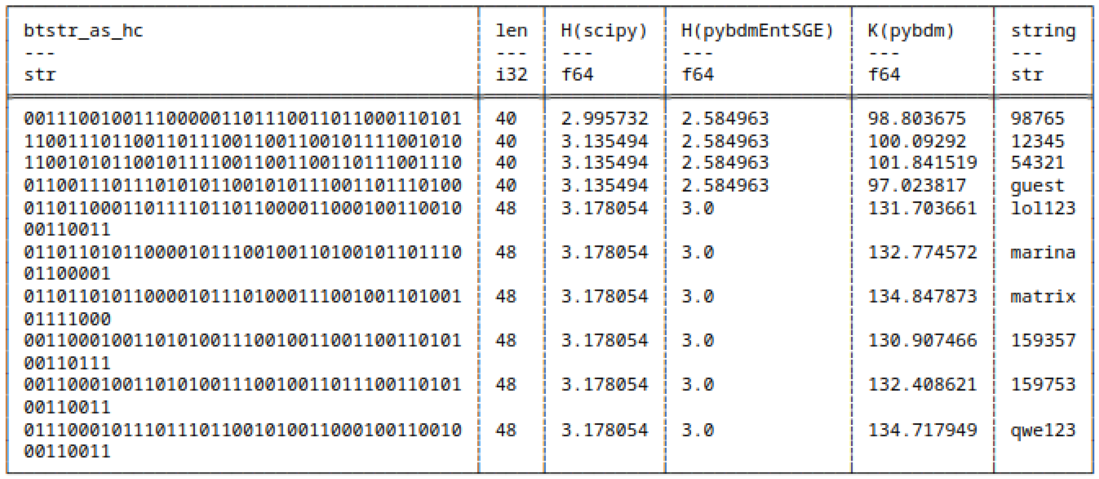
Figure 37.
10 bitstrings with highest H in their HC form - sorted(asc.) on H(scipy).
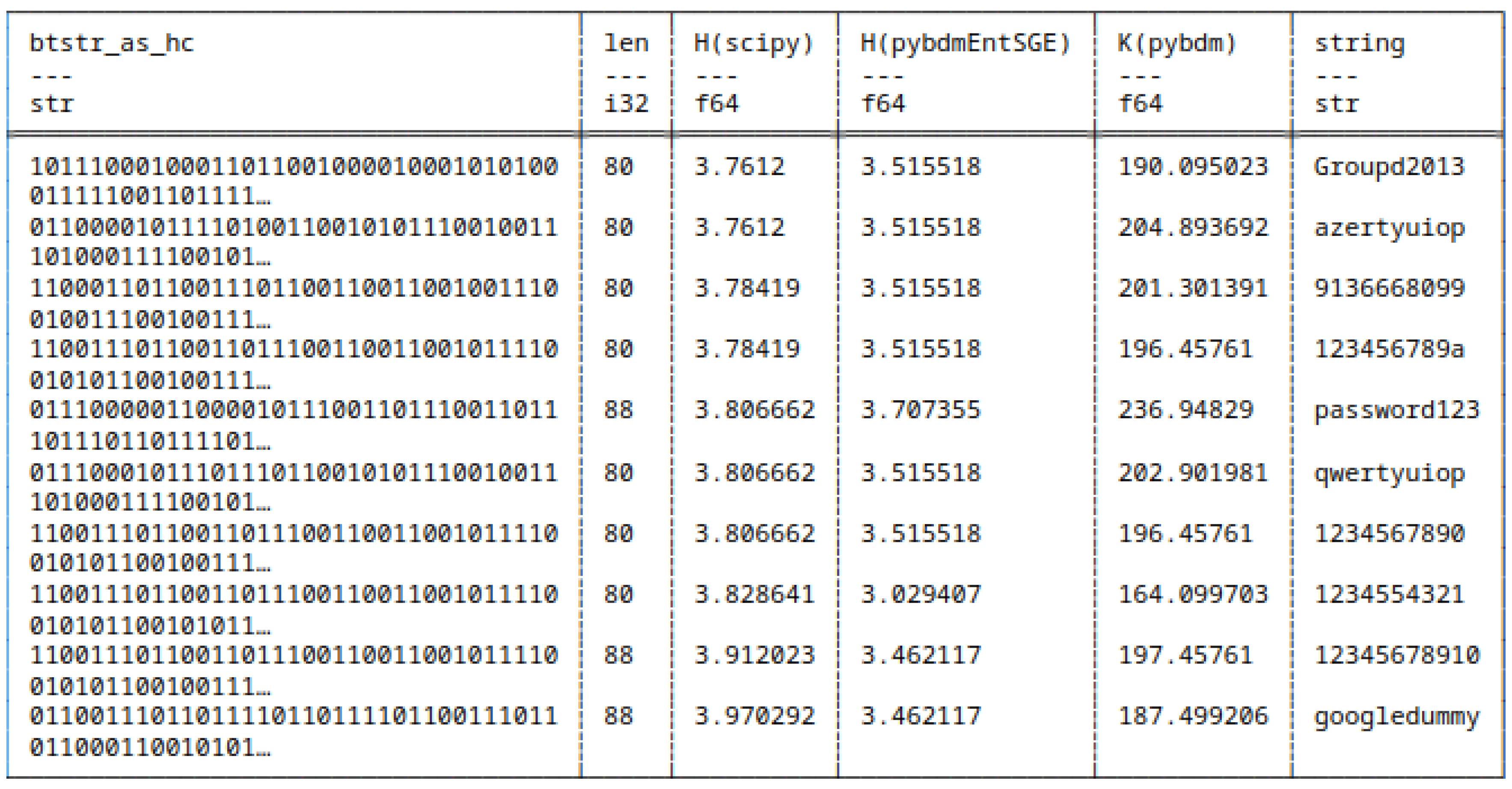
Figure 38.
10 bitstrings with lowest H in their HC form - sorted(asc.) on H(pybdmEntSGE).
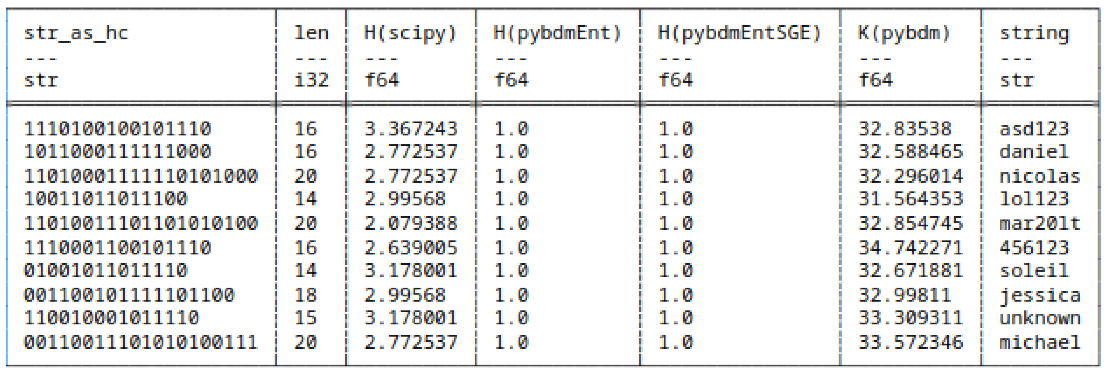
Figure 39.
10 bitstrings with highest H in their HC form - sorted(asc.) on H(pybdmEntSGE).
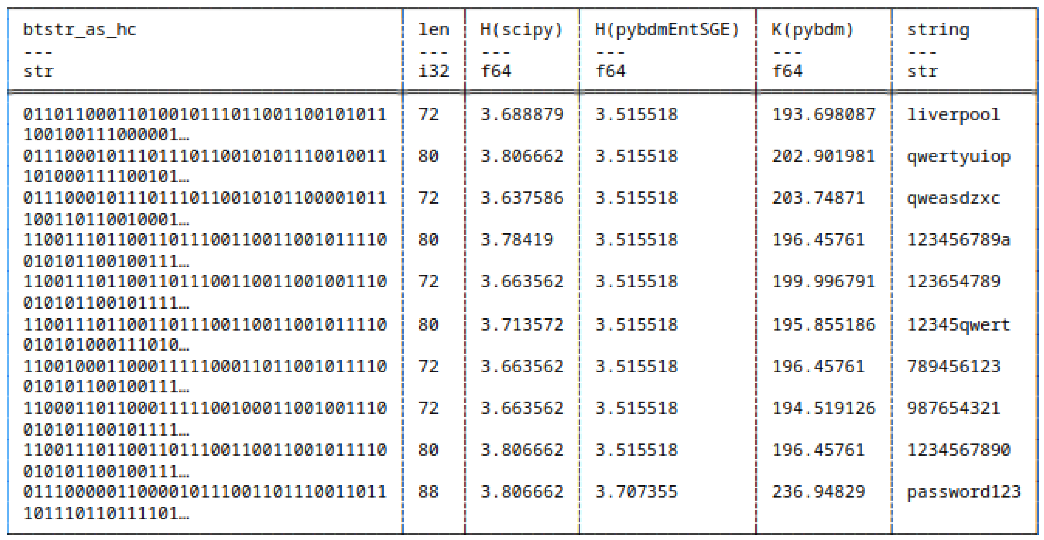
Figure 40.
10 bitstrings with lowest K in their HC form - sorted(asc.) on approximated K(algorithmic complexity).
Figure 40.
10 bitstrings with lowest K in their HC form - sorted(asc.) on approximated K(algorithmic complexity).
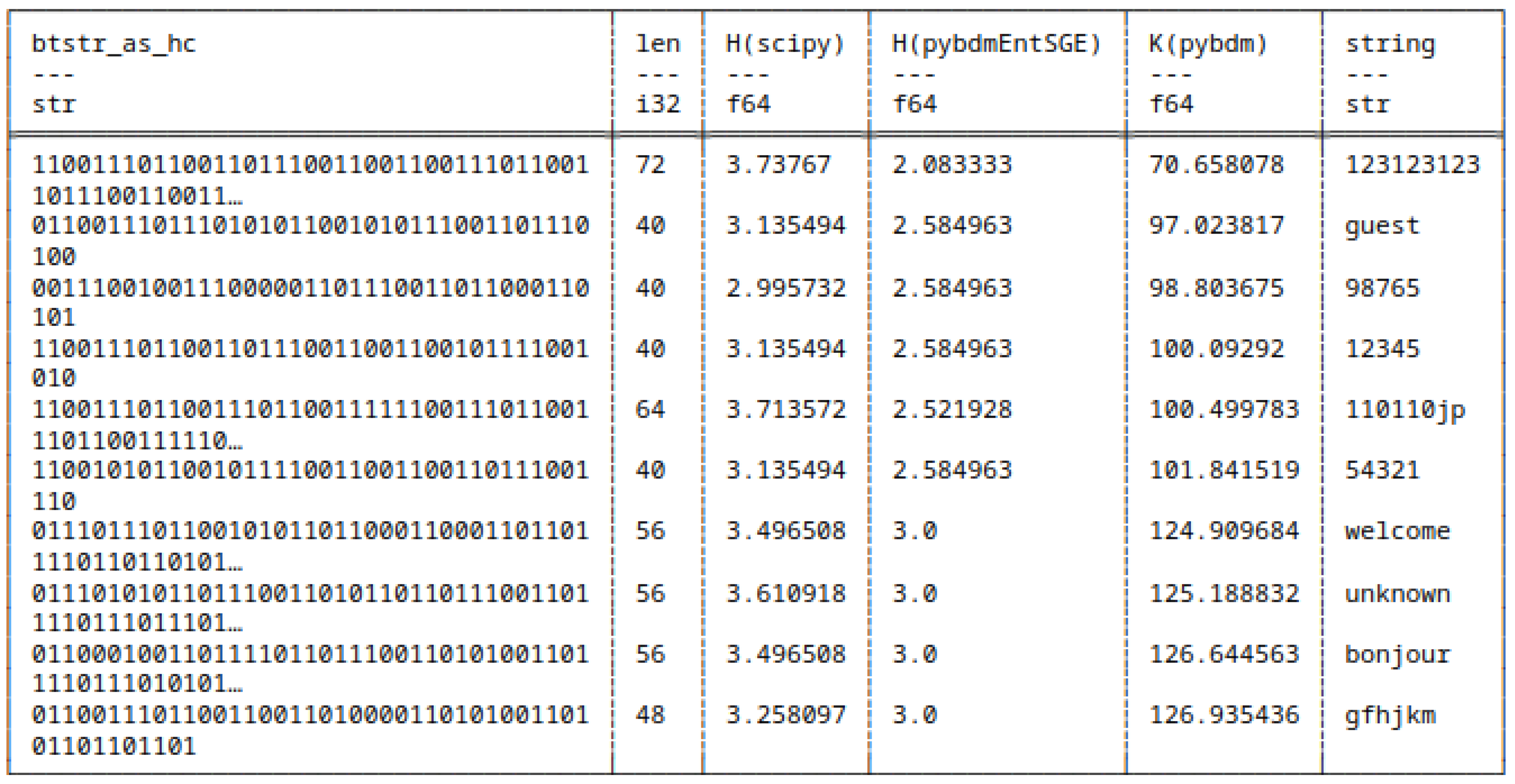
Figure 41.
10 bitstrings with highest K in their HC form - sorted(asc.) on approximated K(algorithmic complexity).
Figure 41.
10 bitstrings with highest K in their HC form - sorted(asc.) on approximated K(algorithmic complexity).
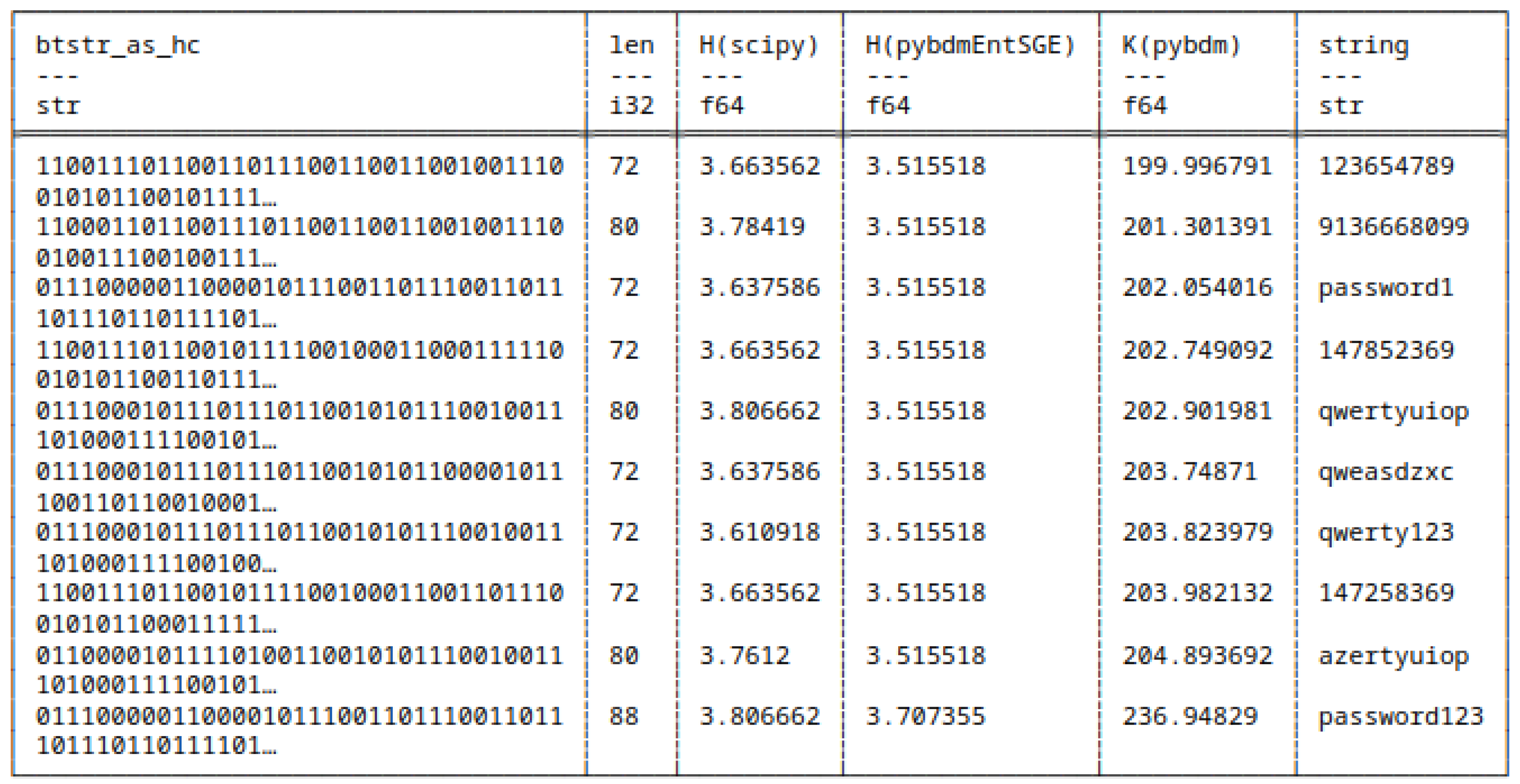
Figure 42.
Descriptive statistics - bitstrings in their HC form.
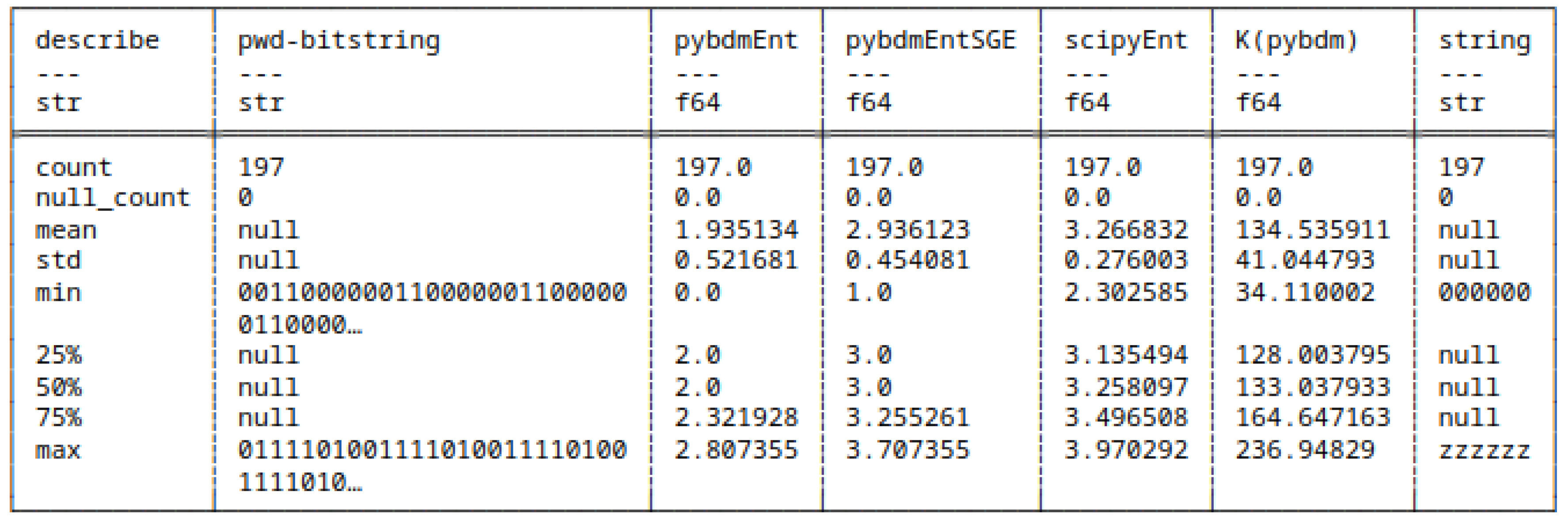
5.8. Shannon Entropy and Algorithmic Complexity of Bitstrings
In this section, we compare how Shannon Entropy and Algorithmic Complexity characterize strings under their bitstring representation.
Figure 43.
10 bitstrings with lowest H - sorted(asc.) on H(scipy).
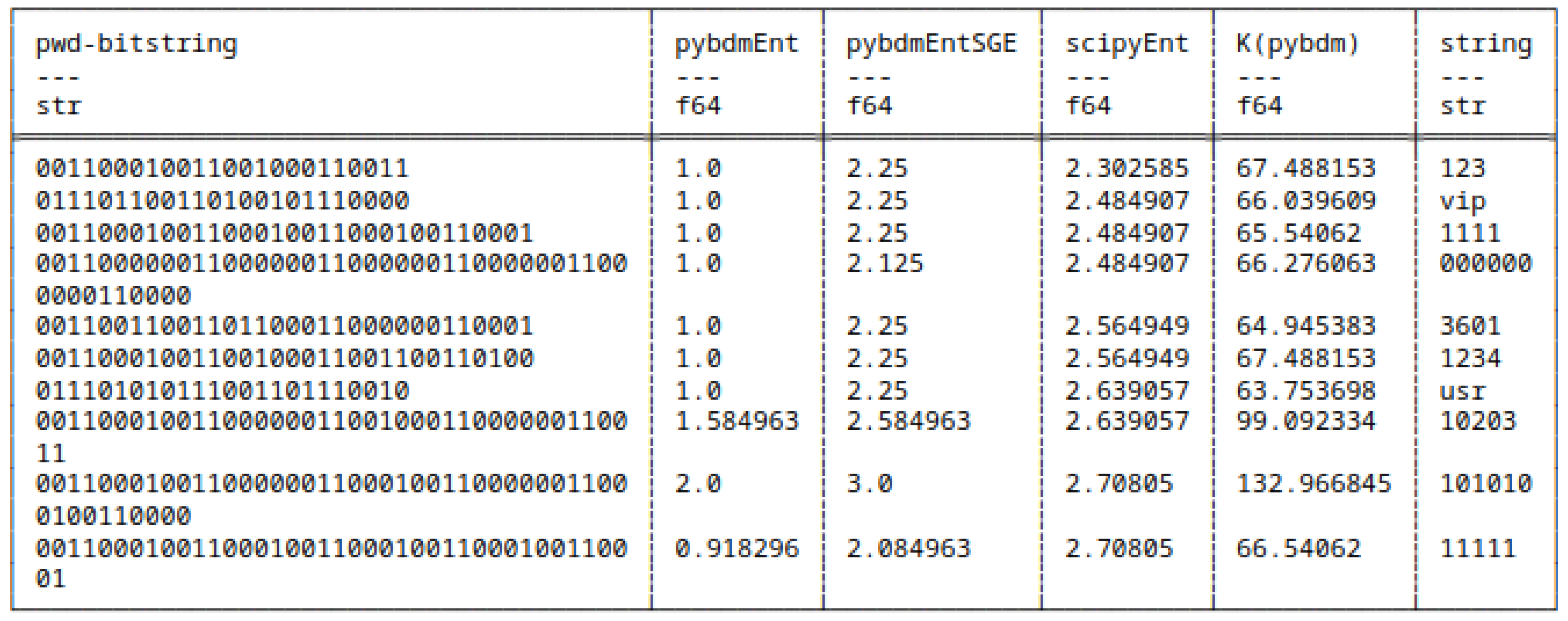
Figure 44.
10 bitstrings with highest H - sorted(asc.) on H(scipy).
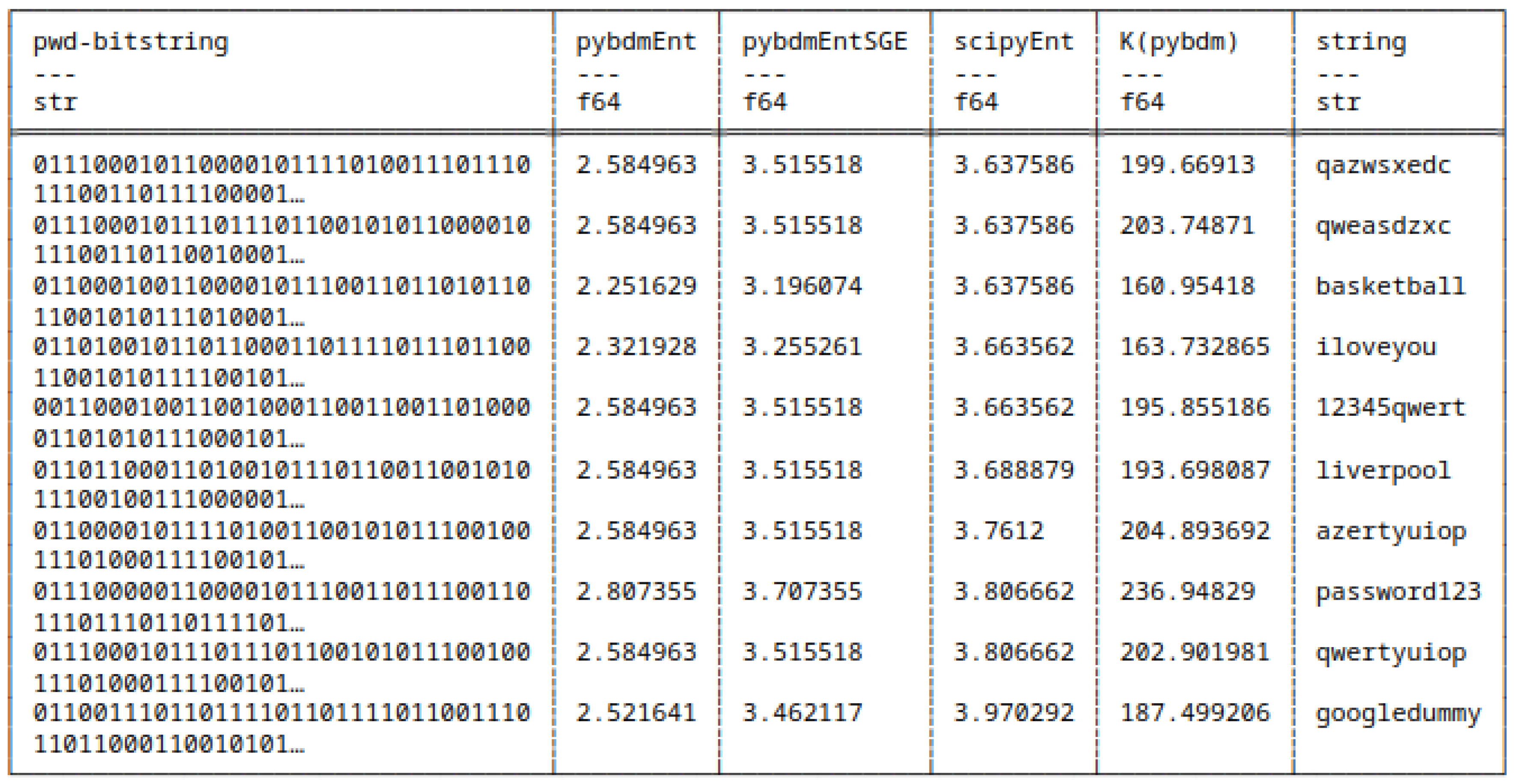
Figure 45.
10 bitstrings with lowest H - sorted(asc.) on H(pybdmEnt).
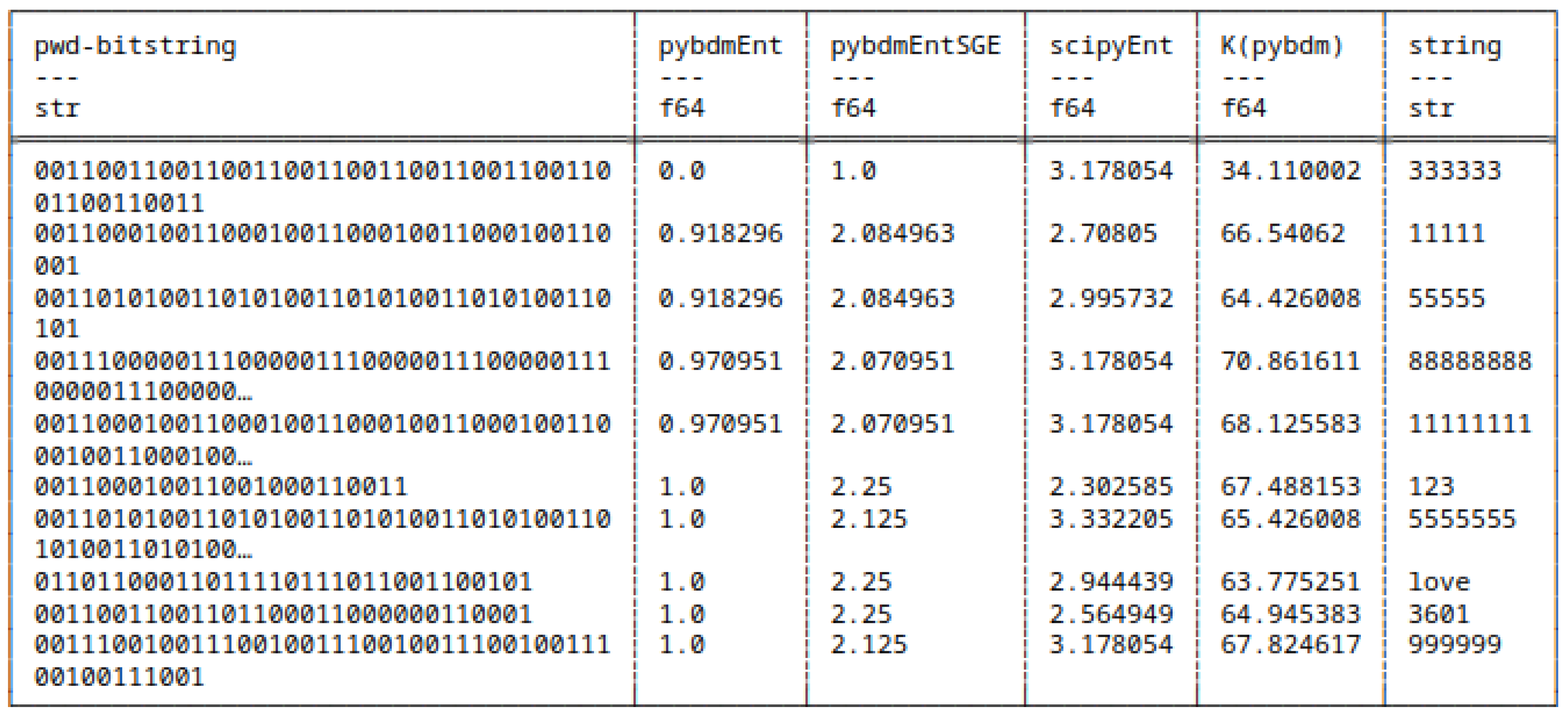
Figure 46.
10 bitstrings with highest H - sorted(asc.) on H(pybdmEnt).
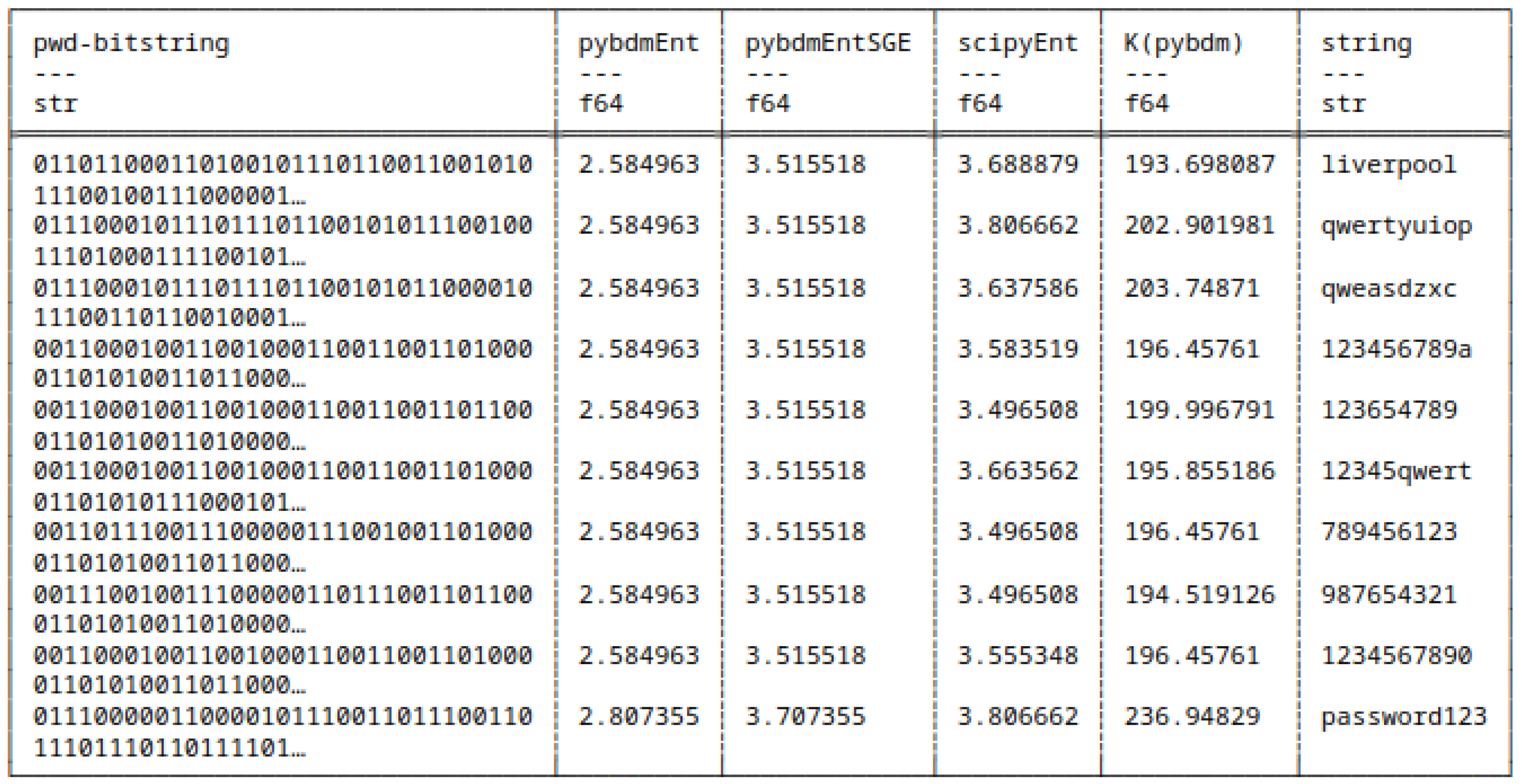
Figure 47.
10 bitstrings with lowest H - sorted(asc.) on H(pybdmEntSGE).
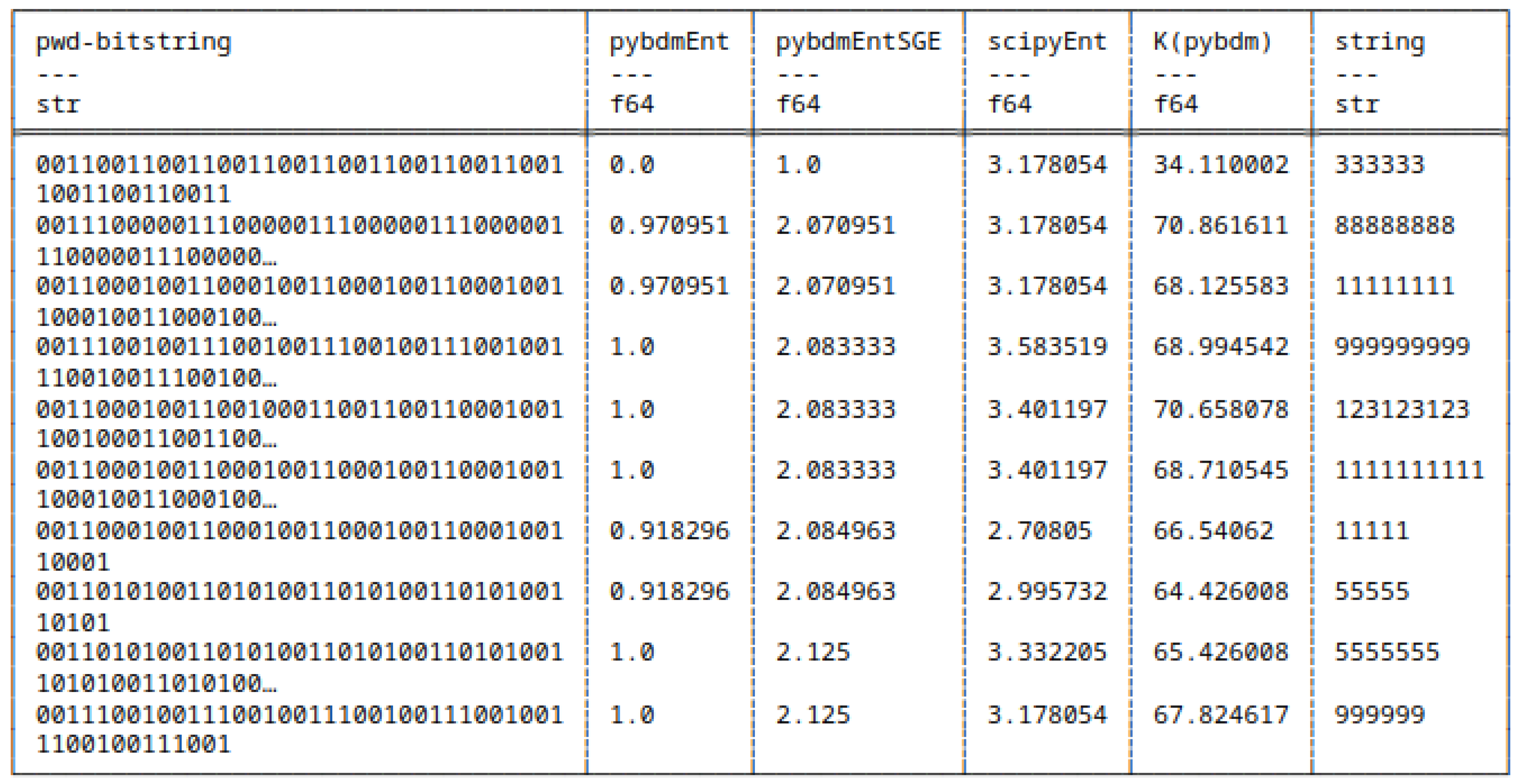
Figure 48.
10 bitstrings with highest H - sorted(asc.) on H(pybdmEntSGE).
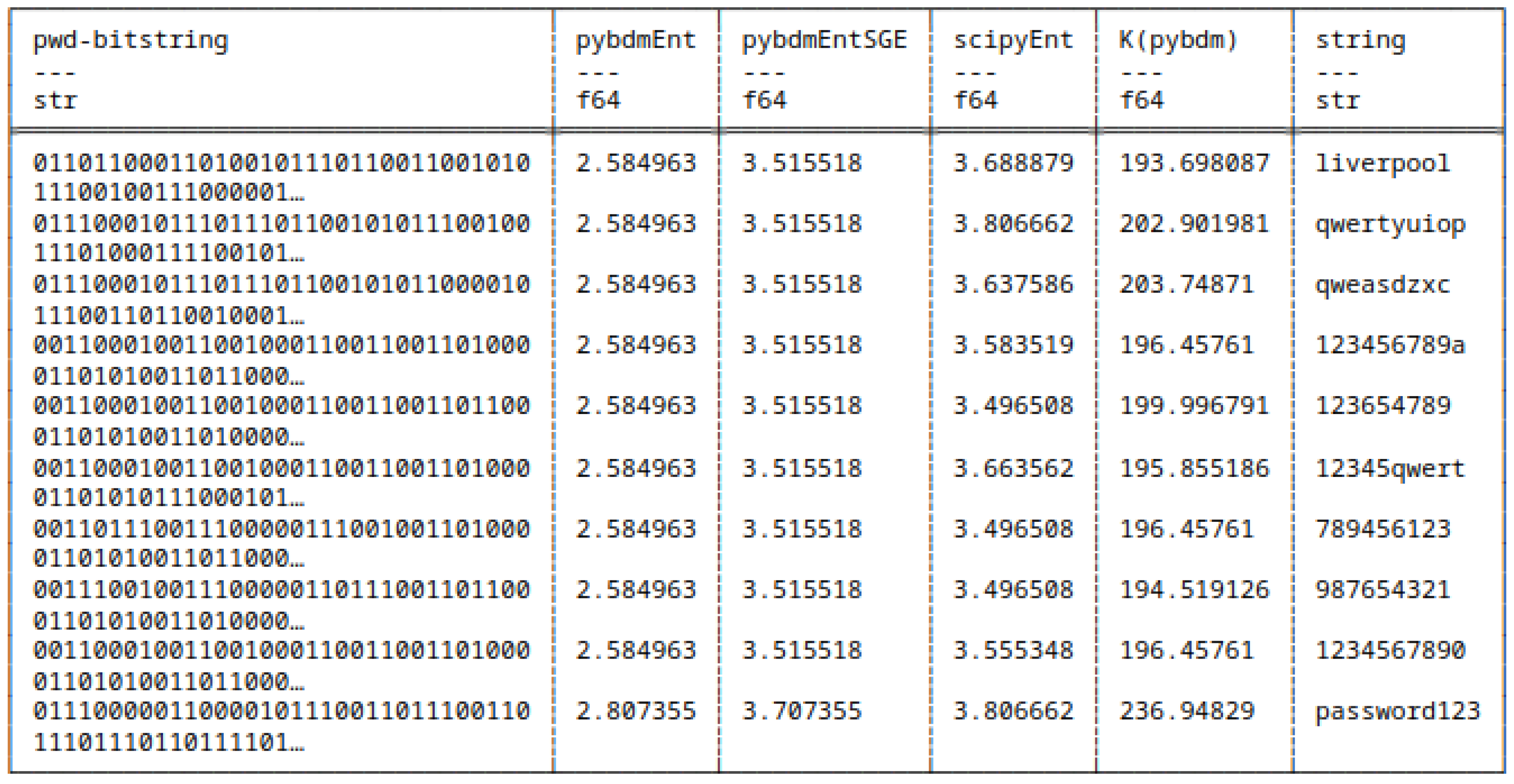
Figure 49.
10 bitstrings with lowest K - sorted(asc.) on approximated K(algorithmic complexity).
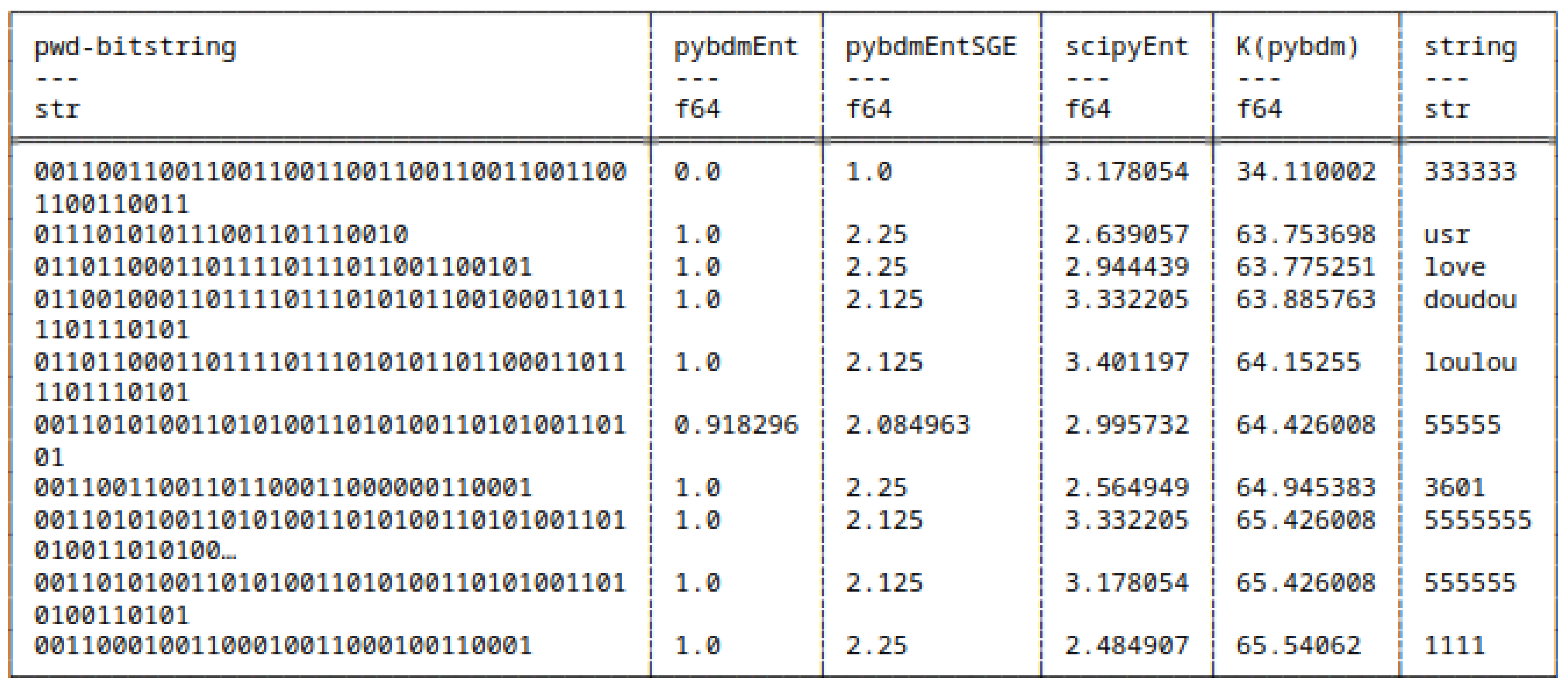
Figure 50.
10 bitstrings with highest K - sorted(asc.) on approximated K(algorithmic complexity).
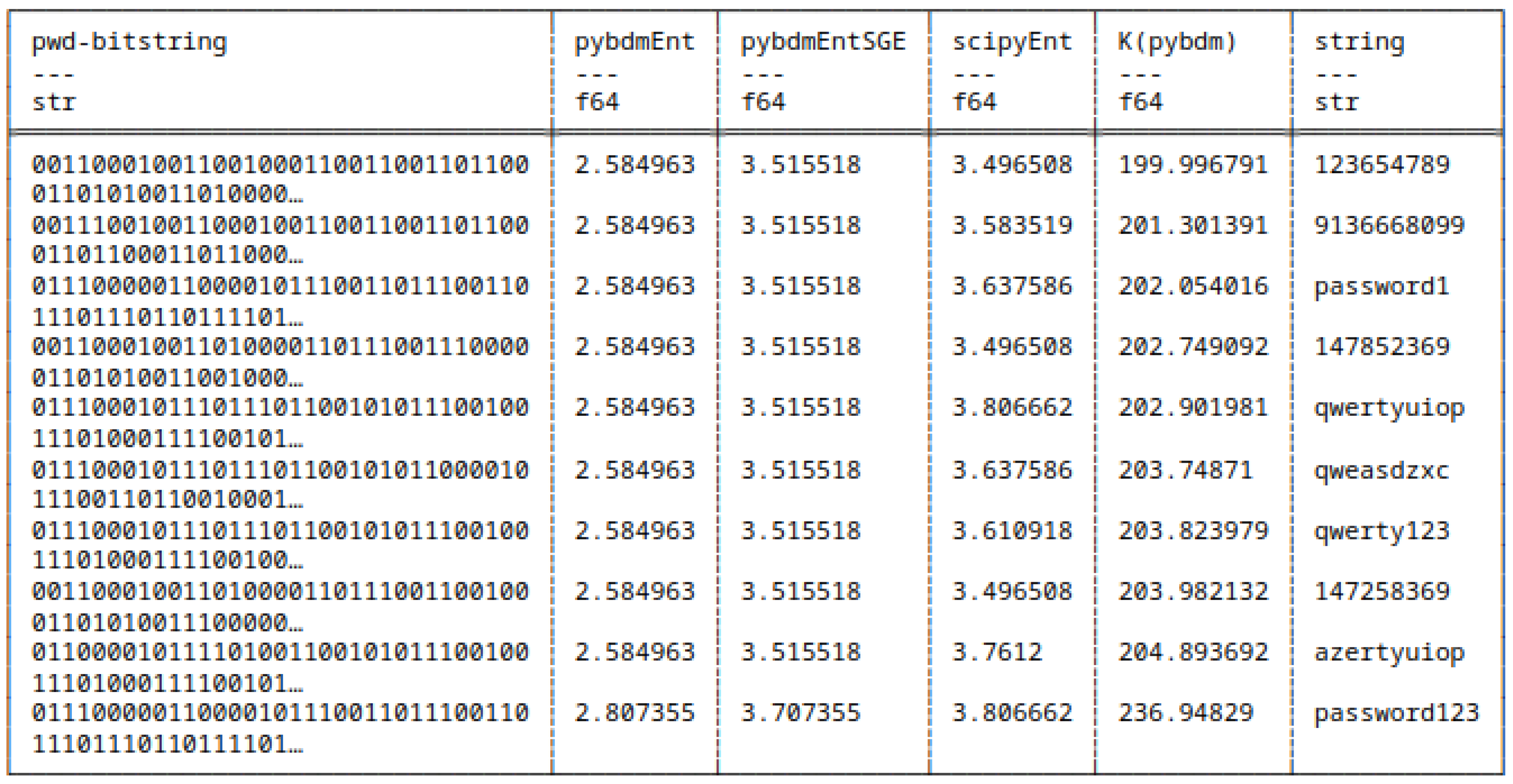
Figure 51.
Descriptive statistics - bitstrings H and K.
5.8.1. Differences in Computing Shannon Entropy
Hereafter, for the passwords bitstring representation, we plot their different entropy values i.e. using the different software packages(Appendix H).
On a purely technical level, we compute different values of Shannon Entropy. Specifically, we compare two existing software packages: pybdm and scipy (details in Appendix H). We bring an additional function into the pybdm package, specifically, we implement the Schürmann-Grassberger estimator, see eq. (7). For convenience purpose, we refer to it as pybdmEntSGE.
Figure 52.
Shannon Entropies of bitstrings using pybdmEnt, pybdmEntSGE, Scipy.
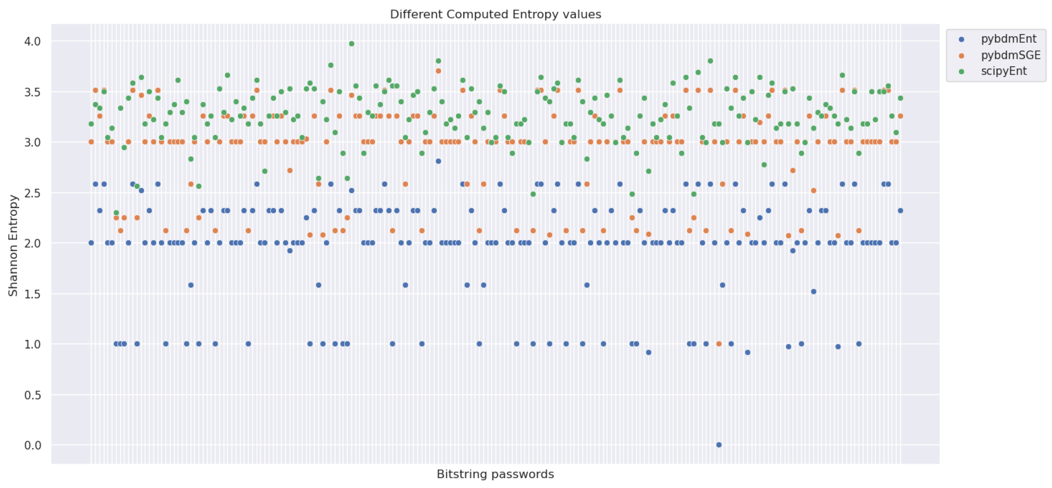
We notice that in general, the pybdmEntSGE implementation has results closer to the ones given by the scipy library.
5.9. Software
References about the software packages are to be found in Appendix H.
5.10. Results
For our experimental setting and based on the data, we report and derive the following results.
The t-test (Section 5.5) shows a significant statistical difference between the mean entropy of strings and their bitstring representation. The difference shows that the mean entropy distribution of strings is lower than their bitstring counterpart. Based on this measure, we can say that the output alphabet in this case {0,1} plays a part in the increase of the computed entropy; the other factor being the length of the object. Indeed, our experiments with RLE brings information about the cardinality of the run-control variables. We observe that on average the strings are of length six. Whereas, it is around thirty for the binary encoding i.e. bitstrings.
Run-Length Encoding is best suited when processing inputs where the same symbol appears consecutively.
From an Algorithmic Complexity perspective, symbols appearing consecutively are said to have low complexity. This is explained by the fact that the concatenation of characters can easily be expressed by a program e.g.: print ’x’*1000. In other words, for a fixed Turing machine, a string where the same symbol is found repeatedly, the length of the program that outputs that type of string is short.
Concerning Huffman Coding, we observed that matching with theory, Huffman Coding can not encode strings with a single symbol. Indeed, in order to be differentiable one needs at least two symbols. Thus, this reduced the number of operable strings to 173. Moreover, because we also wanted to compute their Algorithmic Complexity, the number of computable elements is reduced to 148. In contrast, the space of symbols of bitstrings is two and composed of {0,1}) only.
Regarding the comparison of Shannon Entropy (H) and Algorithmic Complexity (AC) under their bitstring representation, we observe the following elements.
If we consider the extremes i.e.: minimum and maximum, the H and K do not coincide. Moreover, depending on which algorithm is used to compute Shannon Entropy, the agreement in ranking varies.
We first look at the values between the different entropy results. Then, we proceed with a global comparison with the different computed entropies and Algorithmic Complexity.
H and H(pybdmEnt)
for the lowest entropy bitstrings, H based on scipyEnt seems to consider the length of the bitstring as being an impactful factor to characterize low entropy values. Instead, pybdmEnt implementation puts weight on symbol repetitiveness.
H and H(pybdmEntSGE)
for the lowest entropy bitstrings, we only have one match(11111 between the two rankings. For the highest entropy bitstrings, in the scipyEnt case, 8 out of 10 values are composed of characters only; which is 3 for the pybdmEntSGE case. pybdmEntSGE has also 4 bitstrings representing integers only.
The bitstring with maximum entropy is googledummy for scipyEnt and password123 for pybdmEntSGE. Whereas, the bitstring with minimum entropy is 123 and 333333 for scipyEnt and pybdmEntSGE respectively.
H(pybdmEnt) and H(pybdmEntSGE)
for the lowest entropy bitstrings, the values converge on classifying repetitiveness of symbols as a low contributor to the results. However, this is more pronounced in pybdmEntSGE than in pybdmEnt.
For the highest entropy bitstrings, the two implementations concur i.e., the ranking of bitstrings coincide.
H(all approaches) and AC(pybdm)
the difference between Shannon Entropy and Kolmogorov Complexity lies in what criterion impacts low or high entropy/algorithmic complexity. The real contrast is within the low entropy/algorithmic complexity space. Where Shannon Entropy primarily uses the object’s length, Algorithmic Complexity relies on repetitiveness(or the absence thereof) of symbols in the object.
It has to be noted that in general, for the values computed using the pybdm package, there is a number of entropy results having identical entropy values. This is considered in the next Section 6.
In summary, for the scipy implementation of H, it seems that the length of the bitstring plays a heavy weight in the outcome. In contrast, the pybdm implementations of H, i.e.: pybdmEnt(default implementation) and pybdmEntSGE a proposed implementation based on the Schürmann-Grassberger estimator (7) concentrates on same symbol repetitiveness to characterize low entropy. Length has a role but not in conjunction with symbol repetition.
5.10.1. Applicability Shortcomings
Within this section, we discuss the reasons why some processes in the workflow described by Figure 2 could not be computed.
In the Figure 2, there is no arrows for (i) computing the values of the output of Run-Length Encoding; (ii) BDM values for the ASCII representation of passwords.
Concerning (i), it pertains to points: (3) and (9). The output of RLE is composed by two arrays/lists(also called the encoded variable); one containing a single occurrence of a symbol, and the other(also called the run-control variable) containing an integer representing the counts/time of occurrence of that same symbols. This mapping is repeated for each different symbols in the data.
For point (ii), the ASCII symbols are not in the current computed distribution of BDM. We have to resort to the binary representation of strings.
6. Discussion
As mentioned in Section 4.2.2, the Huffman Coding (HC) has been shown to be optimal. Still, it is possible to improve on this result by considering a coding technique such as arithmetic coding and derivative. Indeed, where Huffman Coding uses a full number of bits to encode information, arithmetic coding exploits the interval between zero and one to enhance the compression ratio.
Run-Length Encoding, a finer analysis regarding the cardinality could be an interesting path to explore. ([57,58]).
Regarding the identical values for entropies using the pybdm package, this can be explained because of the implementation rely on the computed distribution for building the distribution.
7. Conclusions
7.1. Why Care About Algorithmic Information Theory?
This writing allowed us to outline some of the features of Algorithmic Information Theory. Its theoretical importance is on par with the field of computability theory. Similarly to Turing’s success to formalize the notion of what it is to compute? with his introduction of "Turing machines"; both Algorithmic Information Theory (AIT) and computational complexity theory formalize the concept of complexity ([4]). Furthermore, in addition of being a part of AIT, Kolmogorov Complexity (K) is also commonly considered as the mathematical formalism of randomness.
However, our prime focus was to have a practical expression of Algorithmic Information Theory. In addition, we wanted to show that this approach was competitive with the foundational Shannon Entropy (H). Besides, Shannon Entropy and Kolmogorov Complexity have commonalities for some properties. This latter aspect is quite interesting but out of the scope of the current analysis. In our study, we reported that one of the cornerstone of AIT i.e. the invariance theorem does not have a correspondence in Shannon Entropy.
7.2. Other Axes of Research
Only considering the previous elements and building upon them, we realise the reach of the field of Algorithmic Information Theory. More specifically, among all the possible development options, we briefly mention the following fields:
- Source coding or data compression,
- Cryptography,
- Program synthesis
These listed items are just a sample of all the possible choices. We selected these fields because of their weight and impact in ”AI”. The common use of Artificial Intelligence (AI) mainly encompasses the sub-fields of: machine learning and deep learning. We posits that there is an untapped potential in the field of Algorithmic Information Theory and some of it’s building blocks e.g.: Algorithmic Probability, Kolmogorov Complexity, Algorithmic Information Dynamics. Finally, the power of Algorithmic Information Theory lies in its universality and, to some extend, in its uncomputability. However,
7.2.1. Data Compression and Computation
Black holes are portrayed as ultimate compressors in ([59]); arguably Algorithmic Information Theory (AIT), and especially, Algorithmic Complexity can be considered as a foundational piece of source coding or data compression.
Indeed, throughout this work, we discussed one of the crux features of Kolmogorov Complexity i.e.: having an agnostic language description(up to an additive constant) for a program.
The core principle of source coding is to have a reduced/compact representation of the input data16. In order to achieve this, lossless compression algorithms(entropy based coding) usually have two components: modelling the language and coding. The former requires having access to the underlying probability distribution of the source sequence. For instance, in the English natural language, this is often approximated by sampling from texts corpus.
Furthermore, in an ideal setting, we would like to have one compression algorithm for all sorts of data. Nonetheless, that would imply to have a "fit them all distribution" for all inputs. That constitutes an object of study on its own: universal source coding. Interestingly, in addition to some common shared properties H and K could find common ground in universal coding ([60]).
On the other side, the path taken by Coding Theorem Method/Block Decomposition Method exploits the whole17 space of two symbols, five states busy beaver machines. This approach lifts the requirement on the underlying probability distribution; which is a desirable property.
Based on the exposed elements and results, it could be interesting to explore the
7.2.2. Cryptography
The field of cryptography is one of the core elements that enables and fuels the development of the information age. The advent and democratisation of cryptography(especially asymmetric key also know as public key) i.e. going from research and some proprietary implementation to the public had been a struggle.
A great deal of information about this subject can be found in ([61]). If we abstract ourselves from the specifics, this is a book about how a piece of technology ”disrupt” a status quo. One of the main element which we can relate to in our current situation with ”AI” is: the regulation system is rather clueless about what is going on and where it is headed(it is already a challenge for some experts). A non-negligible effort is required in order to make these technologies comprehensible and beneficial for the greatest number of persons.
The use of entropy and information theoretic related approaches have been used in different aspects in cryptology, especially cryptanalysis. The chosen approach(CTM/BDM) to algorithmic information theory, specifically to algorithmic complexity could be explored in the space of cryptanalysis. The reliance on entropy based methods and statistical tools could make this field suitable18 to be tackled with AIT. Our exploration showcased the versatility of AIT; thus, by extension and hypothetically, cryptanalytic techniques relying on information theory e.g.: mutual information analysis could benefit from the same approach(with some adaptations).
Finally, another interesting exploration path can be randomness extractors ([62]). These proposals rely on and, are backed by the underlying theoretical framework of Algorithmic Information Theory. To some extent, there is a common set of properties between Information Theory and Algorithmic Information Theory that allows this transfer/application.
7.2.3. Program Synthesis
Software permeates every aspect of our modern societies. One could argue that, a slow but steady merging process is taking place between humans and machines. This hypothesis or evolution, is narrated from a historical and societal lens in The Fourth Discontinuity ([63]).
The ubiquity and reliance on software has been catalyzed by the so-called deep learning revolution ([64]). This has been a moment in history where the conjunction of sufficient availability of data and compute, the exploitation of GPU, triggered the rediscovery of the universal approximation property of feedforward artificial neural networks ([65,66]).
The pervasiveness of software poses the question of their ”maintenance”. Besides, some of these software have reached a size and complexity in terms of lines of code that the qualifications of software stacks and sometimes ecosystems are more appropriate.
This last point sometimes requires humans to develop expertise for a specific application or a reduced set of them. The ability for a single brain to have a decent understanding of several systems is getting tedious. An option to deal with this complexity is through the help of tools, possibly under the form of automation. There is little doubt, that humanity’s history and evolution is intertwined with its ability to wield technology, tools.
This is where the field of program synthesis comes into play. It can be used to offload some parts for maintaining these systems. Naturally, an appealing idea it is to have programs that generate others. The idea is seducing but complex to implement and scale it. Among the different approaches to the field, deep learning and transformer based neural architectures demonstrate serious operational/functional capabilities. One expression of this idea is already in use through: code suggestion and completion in programmer’s IDE19. The use of the Algorithmic Complexity can be used in a hybrid approach to guide the synthesis process.
Acknowledgments
I would like to thank Dr. H. Zenil for remarks regarding the content of this work and suggesting the title for this article.
Conflicts of Interest
The author declares no conflicts of interest.
Appendix H. Software
References
- Talaga, S.; Tsampourakis, K. sztal/pybdm: v0.1.0, 2024. [CrossRef]
- Shannon, C.E. A mathematical theory of communication. Bell Syst. Tech. J. 1948, 27, 623–656. [CrossRef]
- Rényi, A. On measures of entropy and information. In Proceedings of the Proceedings of the Fourth Berkeley Symposium on Mathematical Statistics and Probability, Volume 1: Contributions to the Theory of Statistics. University of California Press, 1961, Vol. 4, pp. 547–562.
- Bennett, C.H. Logical Depth and Physical Complexity. In Proceedings of the A Half-Century Survey on The Universal Turing Machine, USA, 1988; p. 227–257.
- Antunes, L.; Fortnow, L.; van Melkebeek, D.; Vinodchandran, N. Computational depth: Concept and applications. Theoretical Computer Science 2006, 354, 391–404. Foundations of Computation Theory (FCT 2003), . [CrossRef]
- Antunes, L.F.C.; Fortnow, L. Sophistication Revisited. Theory Comput. Syst. 2009, 45, 150–161. [CrossRef]
- Zhou, D.; Tang, Y.; Jiang, W. A modified belief entropy in Dempster-Shafer framework. PLOS ONE 2017, 12, 1–17. [CrossRef]
- Deng, Y. Deng entropy. Chaos, Solitons & Fractals 2016, 91, 549–553. [CrossRef]
- Chaitin, G.J. How to run algorithmic information theory on a computer: Studying the limits of mathematical reasoning. Complex. 1995, 2, 15–21.
- Kolmogorov, A.N. Logical basis for information theory and probability theory. IEEE Trans. Inf. Theory 1968, 14, 662–664. [CrossRef]
- Teixeira, A.; Matos, A.; Souto, A.; Antunes, L.F.C. Entropy Measures vs. Kolmogorov Complexity. Entropy 2011, 13, 595–611. [CrossRef]
- Hammer, D.; Romashchenko, A.E.; Shen, A.; Vereshchagin, N.K. Inequalities for Shannon Entropy and Kolmogorov Complexity. J. Comput. Syst. Sci. 2000, 60, 442–464. [CrossRef]
- Wigner, E.P. The unreasonable effectiveness of mathematics in the natural sciences. Richard courant lecture in mathematical sciences delivered at New York University, May 11, 1959. Communications on Pure and Applied Mathematics 1960, 13, 1–14, [https://onlinelibrary.wiley.com/doi/pdf/10.1002/cpa.3160130102]. [CrossRef]
- Zenil, H. Compression is Comprehension, and the Unreasonable Effectiveness of Digital Computation in the Natural World. CoRR 2019, abs/1904.10258, [1904.10258].
- Li, M.; Vitányi, P. An Introduction to Kolmogorov Complexity and Its Applications, 4th ed.; Springer: Berlin, Heidelberg, 2019.
- Zenil, H.; Kiani, N.A.; Tegnér, J. Algorithmic Information Dynamics - A Computational Approach to Causality with Applications to Living Systems; Cambridge University Press: Cambridge, 2023.
- Chaitin, G.J. A Theory of Program Size Formally Identical to Information Theory. J. ACM 1975, 22, 329–340. [CrossRef]
- Calude, C.S. Information and Randomness - An Algorithmic Perspective; Texts in Theoretical Computer Science. An EATCS Series, Springer, 2002. [CrossRef]
- Rissanen, J. Minimum description length. Scholarpedia 2008, 3, 6727. [CrossRef]
- Wallace, C.S.; Dowe, D.L. Minimum Message Length and Kolmogorov Complexity. Comput. J. 1999, 42, 270–283. [CrossRef]
- Ziv, J.; Lempel, A. A Universal Algorithm for Sequential Data Compression. IEEE Trans. Inf. Theor. 2006, 23, 337–343. [CrossRef]
- Ziv, J.; Lempel, A. Compression of Individual Sequences via Variable-Rate Coding. IEEE Trans. Inf. Theor. 2006, 24, 530–536. [CrossRef]
- Levin, L.A. Laws on the conservation (zero increase) of information, and questions on the foundations of probability theory. Problemy Peredaci Informacii 1974, 10, 30–35.
- Peng, X.; Zhang, Y.; Peng, D.; Zhu, J. Selective Run-Length Encoding, 2023, [arXiv:cs.DS/2312.17024].
- Robinson, A.; Cherry, C. Results of a prototype television bandwidth compression scheme. Proceedings of the IEEE 1967, 55, 356–364. [CrossRef]
- Kelbert, M.; Suhov, Y. Information theory and coding by example; Cambridge University Press: Cambridge, England, 2014.
- Huffman, D.A. A Method for the Construction of Minimum-Redundancy Codes. Proceedings of the IRE 1952, 40, 1098–1101. [CrossRef]
- Levin, L.A. Randomness Conservation Inequalities; Information and Independence in Mathematical Theories. Inf. Control. 1984, 61, 15–37. [CrossRef]
- Rado, T. On Non-Computable Functions. Bell System Technical Journal 1962, 41, 877–884. [CrossRef]
- Delahaye, J.; Zenil, H. Numerical Evaluation of Algorithmic Complexity for Short Strings: A Glance into the Innermost Structure of Randomness. CoRR 2011, abs/1101.4795, [1101.4795].
- Soler-Toscano, F.; Zenil, H.; Delahaye, J.; Gauvrit, N. Calculating Kolmogorov Complexity from the Output Frequency Distributions of Small Turing Machines. CoRR 2012, abs/1211.1302, [1211.1302].
- Zenil, H.; Toscano, F.S.; Gauvrit, N. Methods and Applications of Algorithmic Complexity - Beyond Statistical Lossless Compression; Springer Nature: Singapore, 2022.
- Zenil, H.; Hernández-Orozco, S.; Kiani, N.A.; Soler-Toscano, F.; Rueda-Toicen, A.; Tegnér, J. A Decomposition Method for Global Evaluation of Shannon Entropy and Local Estimations of Algorithmic Complexity. Entropy 2018, 20, 605. [CrossRef]
- Höst, S. Information and Communication Theory (IEEE Series on Digital & Mobile Communication); Wiley-IEEE Press, 2019.
- Cheng, X.; Li, Z. HOW DOES SHANNON’S SOURCE CODING THEOREM FARE IN PREDICTION OF IMAGE COMPRESSION RATIO WITH CURRENT ALGORITHMS? The International Archives of the Photogrammetry, Remote Sensing and Spatial Information Sciences 2020, XLIII-B3-2020, 1313–1319. [CrossRef]
- Zenil, H.; Kiani, N.A.; Tegnér, J. Low-algorithmic-complexity entropy-deceiving graphs. Phys. Rev. E 2017, 96, 012308. [CrossRef]
- Wolfram, S. A New Kind of Science; Wolfram Media, 2002.
- Calude, C.S.; Stay, M.A. Most programs stop quickly or never halt. Adv. Appl. Math. 2008, 40, 295–308. [CrossRef]
- Müller, M. Stationary algorithmic probability. Theoretical Computer Science 2010, 411, 113–130. [CrossRef]
- Calude, C.S. Simplicity via provability for universal prefix-free Turing machines. Theor. Comput. Sci. 2011, 412, 178–182. [CrossRef]
- Savage, J.E. Models of computation; Pearson: Upper Saddle River, NJ, 1997.
- Rojas, R. Conditional Branching is not Necessary for Universal Computation in von Neumann Computers. J. Univers. Comput. Sci. 1996, 2, 756–768. [CrossRef]
- Smith, A. Universality of Wolfram’s 2, 3 Turing Machine. Complex Syst. 2020, 29. [CrossRef]
- Ehret, K. An information-theoretic approach to language complexity: variation in naturalistic corpora. PhD thesis, Dissertation, Albert-Ludwigs-Universität Freiburg, 2016, 2016.
- Bentz, C.; Gutierrez-Vasques, X.; Sozinova, O.; Samardžić, T. Complexity trade-offs and equi-complexity in natural languages: a meta-analysis. Linguistics Vanguard 2023, 9, 9–25. [CrossRef]
- Koplenig, A.; Meyer, P.; Wolfer, S.; Müller-Spitzer, C. The statistical trade-off between word order and word structure – Large-scale evidence for the principle of least effort. PLOS ONE 2017, 12, 1–25. [CrossRef]
- Barmpalias, G.; Lewis-Pye, A. Compression of Data Streams Down to Their Information Content. IEEE Trans. Inf. Theory 2019, 65, 4471–4485. [CrossRef]
- Kolmogorov, A.N. Three approaches to the quantitative definition of information *. International Journal of Computer Mathematics 1968, 2, 157–168, https://doi.org/10.1080/00207166808803030. [CrossRef]
- V’yugin, V.V. Algorithmic Complexity and Stochastic Properties of Finite Binary Sequences. Comput. J. 1999, 42, 294–317. [CrossRef]
- NordPass. Top 200 Most Common Passwords List — nordpass.com. https://nordpass.com/most-common-passwords-list/, 2022. [Accessed 2024-01-06].
- Archer, E.; Park, I.M.; Pillow, J.W. Bayesian Entropy Estimation for Countable Discrete Distributions. Journal of Machine Learning Research 2014, 15, 2833–2868.
- Schürmann, T. Bias analysis in entropy estimation. Journal of Physics A: Mathematical and General 2004, 37, L295–L301. [CrossRef]
- Grassberger, P. Entropy Estimates from Insufficient Samplings, 2008, [arXiv:physics.data-an/physics/0307138].
- Schürmann, T. A Note on Entropy Estimation. Neural Computation 2015, 27, 2097–2106, [https://direct.mit.edu/neco/article-pdf/27/10/2097/952159/neco_a_00775.pdf]. [CrossRef]
- Grassberger, P. On Generalized Schürmann Entropy Estimators. Entropy 2022, 24. [CrossRef]
- Salomon, D.; Motta, G. Handbook of data compression; Springer Science & Business Media, 2010.
- Ilie, L. Combinatorial Complexity Measures for Strings. In Recent Advances in Formal Languages and Applications; Ésik, Z.; Martín-Vide, C.; Mitrana, V., Eds.; Springer, 2006; Vol. 25, Studies in Computational Intelligence, pp. 149–170. [CrossRef]
- Ilie, L.; Yu, S.; Zhang, K. Word Complexity And Repetitions In Words. Int. J. Found. Comput. Sci. 2004, 15, 41–55. [CrossRef]
- Zenil, H. A Computable Universe; WORLD SCIENTIFIC, 2012; [https://www.worldscientific.com/doi/pdf/10.1142/8306]. [CrossRef]
- Grünwald, P.; Vitányi, P.M.B. Kolmogorov Complexity and Information Theory. With an Interpretation in Terms of Questions and Answers. J. Log. Lang. Inf. 2003, 12, 497–529. [CrossRef]
- Jarvis, C. Crypto wars; CRC Press: London, England, 2020.
- Hitchcock, J.M.; Pavan, A.; Vinodchandran, N.V. Kolmogorov Complexity in Randomness Extraction. ACM Trans. Comput. Theory 2011, 3, 1:1–1:12. [CrossRef]
- Mazlish, B. The Fourth Discontinuity. Technology and Culture 1967, 8, 1–15.
- Dean, J. The Deep Learning Revolution and Its Implications for Computer Architecture and Chip Design. CoRR 2019, abs/1911.05289, [1911.05289].
- Hornik, K.; Stinchcombe, M.; White, H. Multilayer feedforward networks are universal approximators. Neural Networks 1989, 2, 359–366. [CrossRef]
- Kratsios, A. The Universal Approximation Property. Ann. Math. Artif. Intell. 2021, 89, 435–469. [CrossRef]
- Van Rossum, G.; Drake, F.L. Python 3 Reference Manual; CreateSpace: Scotts Valley, CA, 2009.
- Vink, R.; de Gooijer, S.; Beedie, A.; Gorelli, M.E.; van Zundert, J.; Guo, W.; Hulselmans, G.; universalmind303.; Peters, O.; Marshall.; et al. pola-rs/polars: Python Polars 0.20.5, 2024. [CrossRef]
- Virtanen, P.; Gommers, R.; Oliphant, T.E.; Haberland, M.; Reddy, T.; Cournapeau, D.; Burovski, E.; Peterson, P.; Weckesser, W.; Bright, J.; et al. SciPy 1.0: Fundamental Algorithms for Scientific Computing in Python. Nature Methods 2020, 17, 261–272. [CrossRef]
- The Sage Developers. SageMath, the Sage Mathematics Software System (Version 9.5.0), 2022. https://www.sagemath.org.
- Wei, T.N. python-rle, 2020.
| 1 | Also known under the name of Solomonoff-Kolmogorov-Chaitin complexity |
| 2 | In this work, we consider the notion of computational as effectively computable or, equivalently computable in a mechanistic sense. |
| 3 | In general, a probability measure is a value within the [0, 1] interval, here it’s called a semi-measure because not every program will halt thus the sum will never be 1. |
| 4 | |
| 5 | Block of information bits encoded into a codeword by an encoder |
| 6 | We will argue its adequation for every context. |
| 7 | in the Shannon sense |
| 8 | In the context of real world computation, this assumption needs to be made. This is in contrast with the theoretical model of a Turing machine which does not made any. |
| 9 | As technically is the Church-Turing Thesis |
| 10 | This probably applies even more to passphrases. |
| 11 | A function f is right-c.e. if it is computably approximable from above, i.e. it has a computable approximation such that for all . |
| 12 | |
| 13 | The reason for this duplicates is unclear, it has been reported. |
| 14 | Also known as the plugin estimator |
| 15 | That is, composed of a combination of characters and numbers |
| 16 | Obviously, there is also the decompression side. |
| 17 | With the help of some heuristics. |
| 18 | Assuming that all Science problems can be seen/recasted as prediction problems then the theoretical power of Algorithmic Information Theory makes it virtually agnostic to any specific field. |
| 19 | Integrated Development Environment |
Disclaimer/Publisher’s Note: The statements, opinions and data contained in all publications are solely those of the individual author(s) and contributor(s) and not of MDPI and/or the editor(s). MDPI and/or the editor(s) disclaim responsibility for any injury to people or property resulting from any ideas, methods, instructions or products referred to in the content. |
© 2025 by the authors. Licensee MDPI, Basel, Switzerland. This article is an open access article distributed under the terms and conditions of the Creative Commons Attribution (CC BY) license (http://creativecommons.org/licenses/by/4.0/).
Copyright: This open access article is published under a Creative Commons CC BY 4.0 license, which permit the free download, distribution, and reuse, provided that the author and preprint are cited in any reuse.


