
Submitted:
14 May 2025
Posted:
15 May 2025
You are already at the latest version
Abstract
As digital transformation becomes an increasingly central focus of national and regional policy agendas, parallel efforts are intensifying to stimulate innovation as a critical driver of firm competitiveness and high-quality economic growth. Yet regional disparities in innovation capacity persists. This study proposes an integrated framework in which regionally tracked digital economy indicators are leveraged to predict firm-level innovation performance, measured through patent activity, across China. Drawing on a comprehensive dataset covering 13 digital economic indicators from 2013 to 2022, the study spans core, broad, and narrow dimensions of digital development. Spatial dependencies among these indicators are assessed using global and local spatial autocorrelation measures, including Moran’s I and Geary’s C, to provide actionable insights for constructing innovation-conducive environments. To model the predictive relationship between digital metrics and innovation output, the study employs a suite of supervised machine learning techniques—Random Forest, Extreme Learning Machine (ELM), Support Vector Machine (SVM), XGBoost, and stacked ensemble approaches. The findings demonstrate the potential of digital infrastructure metrics to serve as early indicators of regional innovation capacity, offering a data-driven foundation for targeted policymaking, strategic resource allocation, and the design of adaptive digital innovation ecosystems.
Keywords:
regional corporate innovation
; patents
; digital economy
; supervised machine learning
; SVM
; random forest
; XGBoost
; ELM
1. Introduction
Over the past decade, China has made notable progress in enhancing its innovation capacity under the framework of its innovation-driven development strategy. According to the Global Innovation Index 2021, China’s ranking in the National Innovation Index rose from 38th in 2000 to 12th in 2020—surpassing the OECD average and making it the only middle-income country among the global top 30. This ascent has largely been fueled by sustained increases in R&D (Research and Development) investment, often captured through patent applications and grants. However, the input-driven nature of this growth raises concerns about its long-term sustainability [1].
The digital economy has emerged as a transformative force, reshaping industry value chains [2] and playing a critical role in driving economic growth and improving energy efficiency [3]. In 2020, China’s digital economy reached CNY 39.2 trillion, accounting for 38.6% of the nation's GDP, with an 8.2% growth rate, positioning it second globally [4]. By 2021, the digital economy further expanded to 45.5 trillion yuan, representing 39.8% of GDP and growing by 16.2% year on year [5]. This remarkable growth underscores the increasing importance of digitalisation in driving economic advancement and efficiency, as evidenced by its expanding contribution to China’s GDP [6,7].
The digital economy promotes high-quality development by enhancing resource allocation efficiency, boosting total factor productivity, and stimulating entrepreneurial activity [8]. Furthermore, it accelerates the integration of digital technologies with R&D systems, profoundly influencing innovation dynamics and the formation of innovation networks [9]. This integration occurs both directly—by improving labor productivity [10] and manufacturing productivity [11]—and indirectly, through the optimization of service sectors [12]. As a result, the digital economy fosters open innovation, enhances human capital, and promotes corporate innovation through improved organizational management and increased demand-driven technological advancement [13]. These innovations, often measured by metrics such as patent filings, demonstrate how the digital economy translates into tangible R&D outcomes.
However, sustaining the momentum of innovation requires substantial investment—often exceeding a firm’s internal financing capabilities [14]. In the rapidly evolving digital landscape, firms must secure additional funding to overcome information asymmetries and financing constraints—needs increasingly met by financial technology (fintech) [15,16]. Digital finance, by enhancing financial flexibility, has been shown to boost R&D investment, particularly among technology-based SMEs [17]. In China, fintech policies have supported sustainable innovation and enhanced business performance without increasing risk [18]. Meanwhile, advances in information and communication technologies underpin a digital economy that fosters growth and productivity, streamlines operations, and broadens access to finance through platforms such as e-commerce [10,11]. The synergy between the digital economy and fintech creates a virtuous cycle: improved credit-asset quality enables financial institutions to assume greater fintech-related risks, fostering non-traditional credit-scoring models and expanding SME credit access [19]. In turn, fintech drives financial inclusion, reduces transaction costs, and accelerates technological progress, reinforcing economic growth and innovation. These dynamics highlight that unlocking the digital economy’s full innovation potential also depends on financing mechanisms to yield measurable innovation outcomes.
China's regional innovation landscape remains uneven, making research and development (R&D) a critical focus for growth. Compared to some developed nations, Chinese firms still have considerable room to enhance their innovation capacity and increase R&D intensity [20]. Moreover, while prior studies document the impacts of the digital economy on aggregate innovation, little is known about how regional digital indicators predict firm-level R&D intensity and patent outcomes. To capture both the inputs and outputs of innovation activity, this study uses patent counts as a proxy for R&D output—the tangible result of inventive processes. The goals of this article are: (1) to examine a comprehensive framework of the mechanisms by which the digital economy drives corporate R&D investment and innovation, through which the relationship between a firm's innovative output and the surrounding digital economy is closely integrated, (2) to evaluate the spatial correlations of these digital economy indicators, which are essential for constructing an informed innovation environment, and (3) to identify and utilize key regionally monitored digital economy indicators to effectively approximate and predict firm-level innovation outcomes.
2. Literature Review
2.1. The Role of the Digital Economy in Enhancing Corporate R&D
The digital economy, initially conceptualized by Tapscott (1996) [21], represents an economic paradigm underpinned by advances in information and communication technologies (ICTs). According to the Chinese government’s 2020 White Paper on the Development of China's Digital Economy, it is characterized by digital knowledge and information as core production factors, digital technologies as drivers of economic activity, and modern information networks as foundational infrastructure [22]. Empirical evidence indicates that the digital economy enhances total factor productivity [23] and contributes substantially to national economic growth [24].
The digital economy exerts its influence on corporate R&D investment through several key mechanisms (Figure 1). First, digital transformation lowers operational costs and improves efficiency, thereby facilitating innovation. Digital technologies streamline production and distribution processes while minimizing energy use, transaction costs, and other operational expenditures [25]. By lowering search, transportation, and validation costs, firms increase profitability and gain greater capacity for R&D investment [26]. Furthermore, digital platforms enhance industrial and supply chain coordination, which in turn supports sustainable economic development and technological innovation [27]. Applications such as the Internet and smart terminals enable real-time, cost-effective information exchange, particularly across geographic boundaries, thereby enhancing processing efficiency. The process of informatization has been linked to productivity gains across multiple sectors, including agriculture [28], manufacturing [11], and services such as retail [29].
Second, the digital economy fosters the development of innovation ecosystems, which are further strengthened by the unique properties of data as a production factor—its virtual nature, non-rivalrous characteristics, and varying degrees of excludability [30]. Strong network externalities enhance information accessibility and reduce barriers to innovation [31]. These attributes facilitate collaborative innovation by enabling multiple entities to derive value from shared datasets. Furthermore, the digital economy supports the formation of industrial clusters through Internet-based platforms, improving economic efficiency through scale effects and technological externalities [32]. Digital transmission enables real-time information sharing across regions [33], overcoming geographic constraints and amplifying knowledge spillovers. Prioritizing data openness maximizes these benefits, broadening access to information and fostering knowledge creation.
Third, the digital economy drives transformation in organizational and sectoral structures. In addition to its technological advantages, it promotes organizational change, facilitates open innovation, and enhances human capital [13]. Corporate innovation is propelled through mechanisms such as open innovation, human capital development, and shifts in organizational management. The role of data in the innovation ecosystem becomes especially transformative when combined with the backward forcing mechanism, where consumer demand and downstream feedback push firms to enhance technological capabilities and accelerate innovation [34]. Resource-dependent industries benefit notably, as the digital economy enables a shift from heavy industries to service-oriented, technology-driven sectors, creating new opportunities for research and development [35]. The integration of the real and digital economies further facilitates the substitution of market capital with social capital, emphasizing interaction and engagement. This fusion amplifies the Pareto-improving effects of digital technology in production, strengthens the synergy between physical and digital R&D, and drives "creative destruction" in traditional industries and market structures [36]. Additionally, open innovation initiatives support the commercialization of emerging technologies, thereby maximizing their economic potential [37].
In summary, the digital economy catalyzes corporate R&D investment by reducing costs, fostering innovation-driven ecosystems, and enabling organizational transformation. These mechanisms highlight its transformative role in advancing technological progress and stimulating corporate innovation. This study uses patent filings as a proxy for R&D outcomes, assessing how the digital economy influences both the scale of R&D investment and its tangible results.
2.2. The Role of FinTech in Advancing R&D Investment
Firm-level R&D is significantly supported by the development of financial technology (FinTech), as innovation activities often require substantial external funding beyond the capacity of internal resources [14]. Firms engaged in intensive R&D typically face high levels of information asymmetry and lack sufficient tangible collateral, leading to credit constraints in traditional financial markets [38]. These constraints are especially pronounced among SMEs, which often lack the “hard” information preferred by conventional lenders—frequently resulting in the abandonment of innovation projects [39,40].
FinTech addresses these challenges by expanding credit access through alternative data sources, including social media activity and big data analytics [37]. Technologies such as big data, cloud computing, and artificial intelligence enable the creation of alternative credit scoring models, thereby improving credit availability for SMEs lacking comprehensive financial records [19]. In addition, FinTech reduces transaction and regulatory costs, increases market liquidity, and enhances financial transparency—alleviating financing constraints for innovation-driven firms [41]. Platforms such as peer-to-peer (P2P) lending and crowdfunding further facilitate direct financing for firms unable to access traditional funding channels [42,43].
By aggregating financial data, expert opinions, and crowdsourced insights, FinTech also reduces information asymmetry and agency problems, fostering both R&D investment and the realization of innovation outcomes, often measured through proxies such as patent filings [44,45]. Moreover, FinTech enhances corporate risk-taking capacity by supporting data-driven decision-making [46,47]. Automated financial algorithms reduce transaction costs and broaden funding possibilities—particularly for larger or more opaque firms—supporting the translation of R&D investments into tangible innovation outputs [48,49]. In China, supportive FinTech policies have stimulated sustainable innovation and business performance, with the number of FinTech firms increasing by 28.08% in 2021—a testament to the growing role of digital finance in fostering R&D investment [50].
2.3. Synergies Between Digital Economy and FinTech in Advancing R&D
FinTech, as a technology-driven financial innovation, remains fundamentally tied to finance and cannot eliminate systemic risks inherent in the traditional financial sector [51]. Compared to financial innovations like asset securitization, FinTech represents a deeper financial transformation [52], carrying a broader range of risks—including network, operational, strategic, and compliance risks.
Improving the quality of credit assets benefits FinTech development, a concept explored within the framework proposed by Chen, Yan, and Chen (2023) [53], which underscores the role of credit asset quality in driving FinTech innovation in the digital economy. China's bank-led financial system makes technological innovation within banks a pivotal factor for advancing the country's FinTech sector. Banks, as primary drivers of FinTech innovation, extend credit while managing risk within defined limits, creating a trade-off between FinTech risk and credit risk: lower credit risk and higher credit asset quality allow for greater tolerance of FinTech risk. Thus, enhancing the quality of credit assets enables banks to engage in more FinTech innovation, advancing development while mitigating associated risks.
The digital economy plays a key role in improving credit asset quality through multiple channels. One major mechanism is fostering economic growth. By enhancing resource allocation efficiency, increasing entrepreneurial activity, and raising total factor productivity, the digital economy drives high-quality economic development [54,55]. This growth environment improves enterprise profitability and solvency, reducing the non-performing loan (NPL) ratio and elevating credit asset quality. As a result, banks are encouraged to allocate resources toward FinTech innovation, ensuring financial stability while minimizing risk.
Additionally, digital technologies, such as ICT, significantly enhance operational efficiency across industries by boosting productivity and reducing costs [10,11]. In the financial sector, these advancements lower transaction costs, facilitate integration between traditional banks and FinTech firms, and eliminate spatial constraints on financial services. This enhances commercial bank efficiency, reduces NPL rates, and streamlines credit delivery, creating an environment conducive to sustained FinTech innovation.
Digital infrastructure, a key component of the digital economy, is also crucial in reducing information asymmetry [56]. By leveraging platforms like e-commerce, the digital economy bridges the information gap between borrowing enterprises and financial institutions. The collaboration between e-commerce platforms and banks introduces an innovative credit model that effectively utilizes SMEs' credit information, minimizing asymmetry between SMEs and banks [57]. This leads to more accurate credit assessments, enhancing financial institutions' ability to implement FinTech solutions efficiently.
As a result, FinTech and the digital economy create a feedback loop that drives R&D investment by firms. Improved credit asset quality supports FinTech advancements in two key ways. First, reduced NPL ratios free up resources for banks to implement innovative technologies, such as alternative credit scoring and automated lending platforms [19]. Second, enhanced credit quality enables financial institutions to tolerate higher levels of FinTech-related risks, spurring the development and integration of FinTech solutions into traditional financial systems. As FinTech expands, it promotes innovation in the digital economy by improving financial inclusion and reducing transaction costs, reinforcing the cycle of economic growth and technological progress. This synergistic relationship demonstrates the digital economy's pivotal role in driving financial and technological advancements, establishing a feedback loop in which improved access to finance fuels R&D investment and drives greater innovation, as evidenced by increased patent activity.
This study proposes that digital economic indices can predict regional patent output, serving as a proxy for R&D outcomes, and may be extrapolated to forecast innovation trends across Chinese provinces. The objectives are: (1) to develop machine learning models for predicting regional patent output based on digital economic indicators; (2) to assess regional associations between key predictors of patent output and their impact on model accuracy and applicability; (3) to compare the predictive performance of four machine learning models—Random Forest (RF), Support Vector Machine (SVM), Extreme Learning Machine (ELM), and XGBoost—evaluating their accuracy and other relevant metrics to identify the most suitable approach; (4) to offer actionable insights for policymakers and businesses to optimize regional innovation strategies using measurable digital economy indicators. These insights will support data-driven development, foster innovation, and guide strategic decision-making at the regional level.
3. Materials and Methods
3.1. Variables Selection and Data Processing
Bukht and Heeks (2017) [58] defined the digital economy as consisting of three interconnected layers: core, narrow, and broad. The core layer includes digital industrial sectors such as IT consulting, software development, telecommunications, and information services. The narrow layer encompasses digital services and the platform economy, while the broad layer extends to areas like e-commerce, the algorithmic economy, mechanized agriculture, and emerging industries [59]. This study specifically utilizes these layers as a foundation for analysis, placing greater emphasis on core layers to ensure they accurately represent the overall digital economy. The selected variables are chosen based on their measurability across regions and their relevance in capturing the digital economic landscape in relation to corporate innovation levels, thereby enhancing the predictive accuracy of the model (Table 1). Patents, measured by the number of patent applications of industrial enterprises, serve as proxies for innovative output, capturing the tangible effects of R&D investments. The variables are sourced from the China Statistical Yearbook and the National Bureau of Statistics.
In total, 14 potential independent variables were selected, including those representing core layer, (7 items) narrow layer (3 items) and broad layers of digital economy (2 items) from 2013 to 2020. Research framework with these factors are indicated in Figure 1. Principle Component Analysis is conducted and Varimax rotation was not applied because the principal components already explained the majority of the variance shown by principle component analysis, and applying such a transformation would not have significantly enhanced the variance structure or the interpretability of the components, or predictive power for the study’s objectives. The suitability test resulted in a Kaiser-Meyer-Olkin (KMO) value of 0.788, exceeding the minimum acceptable value of 0.5 suggested by Kaiser (1974) for factor analysis [60]. The KMO value indicates the proportion of variance in the variables that may be attributed to underlying factors, with higher values suggesting that factor analysis is more appropriate for the data. The result of Bartlett's test of sphericity indicates a chi-square value of 2486.671, with a p-value of 0, suggesting that the correlation matrix significantly differs from an identity matrix and the indicators are suitable for subsequent analysis.
In this study, the input variables are normalized to a [0, 1] range to prepare data for deep learning models. For variables with no negative values, the formula used is:
For variables with negative values, the normalization is done using:
This ensures all variables are appropriately scaled for model training and validation, improving model performance and stability.
3.2. Spatial Relationship of Variables
To uncover spatial relationships in our data, we evaluated spatial autocorrelation for each predictor variable (X) using Moran’s I and Geary’s C. These measures assess the degree of clustering or dispersion across regions, providing insights into the spatial structure of our data. Moran’s I captures global patterns of spatial dependence across all regions, while Geary’s C captures local spatial relationships, showing how each region’s value is related to the values of neighboring regions.
Moran’s I is calculated as:
where is the number of observations, and are the values of the variable at locations and , is the mean of , and is the spatial weight between locations and . Moran's I values range from -1 to +1, where positive values near +1 indicate strong positive global spatial autocorrelation, and negative values near -1 suggest strong negative autocorrelation;
In this formula, the emphasis shifts to the squared differences between neighboring values, making Geary’s C more sensitive to local spatial variation. Geary’s C ranges from 0 to 2, with values closer to 0 indicating strong positive local spatial autocorrelation, while values near 2 reflect strong negative local autocorrelation.
To test the global spatial patterns of CO2 emissions across Chinese provinces, we applied both Moran's I and Geary's C, using an adjacency matrix based on direct neighboring provinces. This matrix, which assigns a value of 1 to adjacent regions and 0 to non-adjacent regions, allowed for the analysis of overall spatial autocorrelation, with Moran's I providing an overall measure of clustering or dispersion, and Geary's C highlighting local variations in spatial relationships.
If significant spatial autocorrelation (p<0.05p < 0.05p<0.05) is detected, it will prompt further testing on model residuals to ensure that spatial effects are adequately captured. Should spatial dependencies remain unaddressed, spatial modeling approaches incorporating geographic features will be employed. These methods allow for the explicit modeling of spatial dependencies, thereby improving the accuracy and interpretability of the findings.
The study employed two complementary spatial weighting schemes—binary and row-standardized matrices. Binary weighting assigns equal influence to all neighboring regions, capturing uniform spatial effects, while row-standardization normalizes weights by the number of neighbors, accounting for such variation in spatial structures. These methods ensure a balanced and accurate assessment of spatial dependencies, guiding necessary model adjustments.
3.3. Machine Learning Models for R&D Prediction
This study employs four machine learning models—Support Vector Machine (SVM), Extreme Learning Machine (ELM), Random Forest (RF), and Extreme Gradient Boosting (XGBoost)—to predict ESG scores in a stacked ensemble configuration. Each model was chosen for its distinct strengths in capturing complex, non-linear relationships within the data.
SVM is effective in high-dimensional spaces, utilizing kernel functions to map data into higher dimensions, while ELM offers computational efficiency by randomly assigning input weights and solving output weights analytically, making it fast with minimal tuning. RF builds multiple decision trees to capture interactions between features, preventing overfitting and improving generalization. XGBoost is included for its advanced gradient boosting capabilities, using both gradient and Hessian information for faster, more accurate updates.
By combining these models, the ensemble leverages their individual strengths, enhancing overall prediction performance for ESG scores. Below, we provide an overview of each model and its integration into the stacking framework.
3.3.1. Support Vector Machine (SVM)
Support Vector Machine (SVM), a supervised learning algorithm, was introduced by Cortes and Vapnik [61]. The core idea behind SVM is to find a decision boundary that maximizes the margin between two classes in a high-dimensional space. This margin maximization allows for the separation of classes with optimal generalization. For nonlinear problems, SVM utilizes kernel functions, which implicitly map input data into higher-dimensional spaces to handle complex patterns. The decision function is given as:
where is the kernel function that replaces the inner product in feature space, are the learned Lagrange multipliers, are the class labels, and is the bias term. In this study, we employ the Radial Basis Function (RBF) kernel, defined as:
The RBF kernel is chosen for its ability to capture complex nonlinear relationships, making it particularly useful when the relationship between input variables and the target is not strictly linear. SVM optimizes the classification boundary by minimizing the hinge loss function while enforcing margin maximization:
where is the weight vector that defines the orientation of the decision boundary, is the bias term that shifts the boundary, and is the regularization parameter that controls the trade-off between maximizing the margin and minimizing classification errors. This ensures that the model generalizes well to unseen data while maintaining robustness to noise and outliers.
3.3.2. Extreme Learning Machine (ELM)
Extreme Learning Machine (ELM), proposed by Guang-Bin Huang, is a single-layer feedforward neural network (SLFN) that differs from traditional neural networks like backpropagation networks (BPN) [62],. Unlike BPN, which requires iterative weight updates, ELM randomly assigns input weights and biases, then analytically determines the output weights, significantly reducing computational cost and training time.
In this study, we employ an SLFN architecture with the following output function:
where is the activation function that maps inputs to the hidden layer’s feature space, and represents the output weight matrix. We utilize the Sigmoid activation function, expressed as:
where and are the randomly assigned input weights and biases, respectively.
ELM’s fast learning speed and minimal parameter tuning make it an efficient choice for our stacking ensemble framework, allowing it to capture complex relationships in the data with reduced computational overhead.
3.3.3. Random Forest (RF)
Random Forest (RF), introduced by Breiman [63], is an ensemble learning method that constructs multiple decision trees to reduce overfitting and enhance prediction accuracy. RF creates an ensemble of trees, where each tree is built using a subset of the training data and features. During the construction of individual decision trees, splits are determined using criteria such as the Gini index or entropy, which measure the impurity or uncertainty within a node. The Gini index for a given split is calculated as:
where pip_ipi is the proportion of class iii within the node. A lower Gini index indicates that the node is more homogeneous, meaning the classes within that node are more pure, which leads to better splits. After constructing individual trees, the margin function for classification in RF is used to assess the confidence of the predictions made by these trees. The margin function is defined as:
where represents the weight assigned to the -th tree, is the indicator function denoting whether the kkk-th tree correctly classifies the input , and represents the maximum weight of misclassifications from other classes. A larger margin value indicates better classification accuracy, reflecting higher confidence in the prediction.
The generalization error is given by:
Thus, while the Gini index influences the creation of each tree by selecting optimal splits based on node purity, the margin function aggregates the predictions of all trees in the forest, contributing to improved classification performance.
To ensure robust predictions, RF optimizes for classification accuracy by utilizing majority voting in classification tasks and minimizes the mean squared error (MSE) in regression tasks:
where is the true value, and is the predicted output. By averaging the predictions across multiple trees, RF reduces variance and improves model stability.
In this stacked ensemble, RF excels in modeling complex interactions and capturing non-linear patterns through its diverse set of trees.
3.3.4. XGBoost
XGBoost, proposed by Chen and Guestrin [64], is a gradient boosting algorithm that builds decision trees sequentially, with each new tree being fitted to correct the errors made by the previous trees. The objective function in XGBoost combines a training loss function and a regularization term to balance model accuracy and complexity. For a given sample , the predicted output is computed as:
where represents the set of decision trees, and is the -th tree. The objective function to be minimized at each boosting iteration is given by:
where is the loss function (often squared error for regression), is the prediction from the previous iteration, and is the regularization term that controls the complexity of the trees to prevent overfitting.
For each tree ftf_tft, XGBoost performs a second-order optimization using both the gradient and Hessian of the loss function. Specifically, the gradient and Hessian are computed as follows:
Gradient:
Hessian:
These are used in the update step of the boosting algorithm to adjust the tree's weights and minimize the objective function more efficiently. By incorporating both first- and second-order derivatives, XGBoost can make faster and more accurate updates to the trees, enhancing model performance.
XGBoost's ability to fine-tune the construction of its trees through gradient-based optimization and regularization makes it an essential component of the stacked ensemble model.
3.4. Stacking Ensemble
To enhance the predictive power of individual models, we employ a stacked ensemble approach, combining the outputs of SVM, ELM, RF, and XGBoost. The predictions from each model are used as input features for a meta-model, which makes the final prediction. This meta-model leverages the strengths of each base learner, thereby improving the overall performance in ESG score prediction. The equation for the stacking ensemble approach can be represented as:
Where denotes the final prediction made by the stacking ensemble for the -th instance. The terms represent the predictions made by the base models, which in this case are SVM, ELM, RF, and XGBoost. If the meta-model combines the outputs linearly, the equation can be further specified as , where represents the weight assigned to the prediction of the -th base model. The function is the meta-model that takes the outputs of these base models as input features and generates the final prediction. This formulation effectively leverages the strengths of individual base models while improving overall predictive performance through the meta-model.
Stacking helps reduce bias and variance. By combining diverse models, it mitigates the risk of overfitting associated with individual models, providing a more stable and generalized prediction. This process theoretically reduces model bias by compensating for individual weaknesses and stabilizes variance through ensemble averaging, leading to more robust performance.
3.5. Model Training and Validation
All models were trained on a training dataset spanning from 2011 to 2020. For each model analyzed, the same methodological steps were applied, customized for the specific features of the model. Initially, the dataset was filtered to exclude rows with zero values for CO2 emissions and any rows where independent variables contained zero values. This preprocessing step ensured that only valid data was used for model training. Next, the data was split into training (70%) and testing (30%) sets using a random partition, ensuring an appropriate representation of the data in both sets for final model evaluation.
Hyperparameter optimization was performed using a 5-fold cross-validation approach. In this method, the training dataset was divided into five subsets, and the model was trained and validated five times. Each fold served as a validation set once, with the remaining four folds used as the training set. This cross-validation process allowed for a robust evaluation of model performance across different subsets of the data. To fine-tune each individual model, GridSearchCV was employed, which tested multiple combinations of hyperparameters. The grid searched through different values for key parameters, such as the learning rate, maximum tree depth, number of estimators, subsample rate, and column sample by tree, to identify the best configuration for optimizing predictive accuracy.
In addition to the tuned models, the study included non-tuned models with default hyperparameters as a baseline for comparison. This approach allowed us to assess whether hyperparameter optimization led to significant improvements in predictive accuracy, or if the default settings were sufficient. The comparison also highlights the trade-off between the computational cost of tuning and the potential gains in model performance.
Once the individual models were optimized, model stacking was implemented to further improve predictive performance. The stacking approach involved training multiple base models, each fine-tuned through the aforementioned hyperparameter search, and combining their predictions using a meta-model. The base models tested in this study include Random Forest, Gradient Boosting, Support Vector Machines (SVM), and Extreme Learning Machines (ELM), each contributing unique learning strengths. The meta-model was trained on the predictions made by the base models, including Linear models, Tree-based models (e.g., Random Forest, Gradient Boosting) for flexibility in capturing non-linear relationships, and Neural Networks for complex pattern recognition. The study identifies the most accurate configuration. The stacked model thus leverages the strengths of each individual model while mitigating their weaknesses.
The final model, trained with the best hyperparameters found through GridSearchCV and stacking, was then evaluated using various performance metrics, including RMSE, MAE, MAPE, SMAPE, MdAPE, and R², both on the training and testing datasets. Additionally, statistical significance was assessed through a one-sample t-test to compare the predicted values with the actual values and determine if there were any systematic biases. These metrics and statistical tests provided insight into the model’s accuracy, robustness, and generalization ability, ultimately identifying the most suitable configuration for predicting the target variable.
Overall, this methodology ensured a thorough examination of the model's ability to predict CO2 emissions across various data splits and provided insights into its stability and generalization capacity.
3.6. Testing and Performance Evaluation
After training and validation, each model was evaluated on the testing set from 2022 to assess its generalization ability. The models' predictions were compared with actual R&D outcomes for the year 2022. To quantify model performance, several evaluation metrics were computed, including Mean Error (ME), RMSE, and R². Additionally, cross-validation diagrams were generated to visualize the consistency and accuracy of each model. These metrics helped in understanding how well each model generalized to unseen data.
The performance of the stacked model is evaluated using three error metrics: Root Mean Squared Error (RMSE) (1), Mean Absolute Error (MAE) (2), and Median Absolute Percentage Error (MdAPE) (3). These metrics are defined as:
where represents the actual value and the predicted value. These indices helps assess both the precision and robustness of the stacking ensemble across various test scenarios. RMSE measures the average magnitude of errors, penalizing larger deviations more heavily, where lower values indicate better model performance. MAE provides the average absolute error, offering a simpler interpretation of accuracy with less sensitivity to outliers. MdAPE expressed as a percentage, measures the typical percentage error between predicted and actual values by taking the median of the absolute percentage errors. Unlike mean-based metrics of Mean Absolute Percentage Error (MAPE), which averages the errors and can be overly influenced by extreme values, MdAPE provides a stable measure and robust indicator of forecast accuracy by focusing on the central tendency of the errors. These metrics collectively provide a comprehensive evaluation of the models' predictive accuracy and reliability (Table 2).
Significance tests using p value is utilized to assess whether the predicted values generated by the machine learning models significantly differ from the actual observed target values. The null hypothesis (H₀) assumes there is no significant difference between the predicted and actual values, while the alternative hypothesis (H₁) suggests that such a difference is significant. To test this, we used a 95% confidence level (α = 0.05), where the null hypothesis would be rejected if the p-value is less than 0.05.
The trained models, including the stacked model, were then applied to predict future R&D outcomes for the estimating sub-dataset covering the period from 2023 to 2024. Predictions were made for each of the regions based on the historical data and the optimized model configurations. The forecasting ability of each model was evaluated using the same performance metrics as in the testing phase. The predicted future R&D outcomes were then compared to the actual outcomes to assess the accuracy and reliability of the models' forecasts.
4. Results
4.1. Spatial Correlation Analysis
Table 3 summarizes spatial autocorrelation in key variables was assessed using Geary’s C and Moran’s I indices, with results for both binary and row-standardized results displayed. The small mean Geary's C values suggest weak local spatial autocorrelation for the variables, indicating that the spatial relationships are more globally distributed or less pronounced at local scales, as compared to the Moran’s I index, which captures more generalized spatial patterns.
Meanwhile, three of the digital economy indicators showed significant spatial autocorrelation Moran’s I indices, which reflect broader spatial trends in economic and demographic factors, with proportions significant across all years and consistent patterns across time and correlation indicated at both the binary and row-standardized levels. Based on row standard weight types, Digi_Econ and Tele_Bus show Moderate positive spatial autocorrelation (Moran’s I = 0.3851 and 0.4175 respectively), Population show moderate positive spatial autocorrelation(Moran’s I = 0.2804), while R_D_Fund only show a mild tendency for neighboring locations to have similar values (Moran’s I = 0.19960922).
Figure 2 illustrate the significance, degree of Moran’s I and its temporal trends for each variable over the years, with higher values indicating stronger positive spatial autocorrelation. Over time, Moran's I values revealed a general decline in the spatial autocorrelation of patents, suggesting a growing negative spatial autocorrelation. This indicates that regions with high values are increasingly located near regions with low values, reflecting a reduction in global spatial dependence. Conversely, an increasing trend in global spatial clustering was observed for fiber_cable_density, while it_service_gdp showed a consistent upward trend, with Moran's I becoming significant around 2018. Telecom_gdp demonstrated a sharp increase in spatial autocorrelation from 2017, indicating stronger regional clustering since that time. In contrast, rd_funding and mobile_base_density remained relatively stable, with little change in their spatial patterns. This shift in Moran's I values highlights the evolving spatial dynamics of technological and economic indicators over the years, suggesting a changing landscape of regional interdependence and spatial distribution.
Given that only 4 out of the fourteen variables exhibit significant yet weak to moderate spatial dependencies, incorporating spatial dimensions into the machine learning model is deemed unnecessary, as the spatial relationships are not widespread across the dataset.
4.2. Machine Learning Outcomes
4.2.1. Model Parameters
This study employed ELM, RF, and SVM models using MATLAB 2021, and the XGBoost model was implemented in Python 3.10 due to the absence of a native XGBoost toolbox in MATLAB. The ELM model, a single hidden layer neural network, was configured with 30 hidden nodes—determined through trial-and-error—and used the sigmoid function as the feature mapping function. Other parameters remained at default values.
The Random Forest model was constructed using the TreeBagger function in MATLAB with 20 decision trees. The model was set to perform regression with feature split points selected based on curvature. The SVM model utilized MATLAB’s fitrsvm function with a linear kernel, and default settings were applied to remaining parameters. The XGBoost model was implemented in Python with the gbtree booster. Key parameters included a learning rate of 0.1, max_delta_step of 5 to aid convergence, and 500 boosting iterations. Parallel tree construction was set to 1, limiting the model to sequential training. For model stacking, two ensemble approaches were explored. The first, "Stacked Model (Full Ensemble)," combined predictions from XGBoost, RF, SVM, and ELM using XGBoost as the meta-learner. The second, "Stacked Model (RF + XGBoost)," used predictions from RF and XGBoost combined via a linear regression meta-learner.
The parameters for all base models, as well as meta-learners used in ensemble models, are summarized in Table 4.
4.2.2. Empirical Prediction Results
Based on Table 5, all four machine learning models achieved high predictive performance on the testing set, with R² values exceeding 0.93. While the RMSE, MAE, and MdAPE values varied across models, they consistently remained low, indicating robust accuracy and generalization capability. Statistical significance was assessed using t-tests to determine whether the predicted values significantly differed from the actual observed target values. For all models tested, the p-values were greater than the 0.05 significance threshold, suggesting that the null hypothesis (no significant difference between predicted and actual values) could not be rejected, indicating no systematic bias in the predictions.
Among the evaluated models, the stacked ensemble combining XGBoost and Random Forest demonstrated the best overall predictive performance on the testing dataset. As shown in Table 1, this model achieved the lowest RMSE (0.0247) and MAE (0.0137), alongside a high R² value of 0.9791, indicating strong predictive accuracy and a close fit to the observed values. It also maintained a relatively low MdAPE of 17.62%, highlighting the stability of its predictions.
While the standalone XGBoost model also performed well, with an RMSE of 0.0253, MAE of 0.0136, R² of 0.978, and MdAPE of 16.84%, the stacked XGBoost-RF ensemble slightly outperformed it across most metrics. In contrast, models such as SVM and ELM, despite achieving high R² values (0.9501 and 0.973, respectively), exhibited higher error magnitudes, particularly in MdAPE, suggesting lower consistency in prediction accuracy.
The fully stacked model incorporating all base learners (XGBoost, Random Forest, SVM, and ELM) also showed reasonably good performance (RMSE = 0.0299, MAE = 0.0146, R² = 0.9694, MdAPE = 18.70%), but did not surpass the more targeted XGBoost-RF ensemble.
These results are further illustrated in Figure 3, which provides a normalized visual comparison across models based on R² (inverted), RMSE, MAE, and MdAPE. For consistency in interpretation, all metrics were scaled to a [0, 1] range using min-max normalization, where lower values indicate better performance. Since higher R² values represent better fit, the normalized R² values were inverted (1 – normalized R²) to align directionally with the error metrics. The XGBoost-RF stacked model achieved the lowest average normalized score across all metrics, reinforcing its selection as the most suitable model for predictive modeling in this study due to its optimal balance of accuracy and generalization on unseen data.
The line charts (Figure 4) display the actual values and predicted values of ELM, RF, SVM, and XGBoost models for both the training and testing datasets over the entire period of 2013 to 2021.
5. Discussions
For regional governments, the ability to predict patent outputs based on digital economy indicators is an essential tool for informed decision-making. This study aimed to investigate the intricate relationships between regional digital economy indicators and the innovation performance of firms, as measured by patent output, within the context of China's evolving innovation landscape. The study's models—backed by strong predictive accuracy—allow policymakers to forecast innovation trends and identify regions where digital economy investments, such as expanding broadband networks or fintech infrastructure, are likely to yield the greatest impact. These models can inform targeted policies that foster R&D, attract talent, and boost collaboration among firms in emerging innovation clusters.
The spatial correlation analysis provides valuable insights into the regional dynamics of digital economy and innovation outcomes, particularly with respect to patent production. Only 4 out of the 14 key variables (Digi_Econ, Tele_Bus, Population, and R_D_Fund) exhibited significant spatial autocorrelation, and even these relationships were relatively weak to moderate. This indicates that the majority of digital economy and innovation indicators do not show strong spatial clustering, reducing the necessity for spatial modeling.
The Moran’s I index for patents showed a general decline over time, suggesting increasing spatial heterogeneity in innovation output. High-performing regions are less likely to be geographically clustered with other high performers, pointing to a decentralization of innovation activity. For policymakers, this decentralization highlights the importance of fostering innovation beyond the well-established hubs. Localized initiatives and policies that promote regional innovation can help ensure that even geographically distant areas can compete in the innovation landscape.
While the overall spatial autocorrelation for digital economy indicators remained weak, certain variables, such as telecom infrastructure (fiber cable density) and IT service GDP, exhibited stronger spatial clustering trends. This indicates emerging spatial clustering trends in technological infrastructure and services, possibly reflecting regional specialization or targeted investments. These regions may attract investments in infrastructure, fostering innovation ecosystems that encourage knowledge spillovers and collaboration. For regional governments, these emerging clusters offer an opportunity to target investments and policies that support local technological development. By identifying regions with growing tech infrastructures, policymakers can facilitate the development of specialized digital ecosystems that are likely to drive regional patent output and innovation.
Traditional R&D inputs, such as R&D funding and mobile base station density, showed stable spatial patterns over time, indicating that these factors are less influenced by geographical proximity and more shaped by institutional or policy-driven decisions. This finding suggests that while R&D investment might not be directly dependent on regional clustering, it is still crucial to maintain a stable flow of funding and infrastructure development across regions. Policymakers can use this insight to ensure that the regions with established R&D frameworks continue to receive the necessary support, fostering sustained growth in innovation and maintaining regional competitive advantage. In this context, the study’s predictive models can help assess areas where investment in traditional R&D is necessary to maintain innovation momentum.
Given that the spatial relationships between innovation outputs and the digital economy indicators are not strongly spatially dependent across most regions, regional governments can still rely on the general predictive power of the digital economy indices—such as ICT infrastructure, fintech development, and R&D investment—to forecast regional patent outcomes. The absence of significant spatial autocorrelation suggests that machine learning models, such as those developed in this study, can be applied across various regions without the need for complex spatial modeling. These models can predict patent activity based on digital economy metrics, offering regional policymakers a tool to assess and monitor innovation potential in their areas.
Furthermore, the study integrates insights from the fintech sector, which has become a key enabler of innovation financing. The literature emphasized that fintech reduces financing barriers by addressing information asymmetry and improving access to capital, particularly for SMEs. The empirical results validate this by showing that the synergy between the digital economy and fintech plays a pivotal role in driving R&D investment and, ultimately, innovation output. Our models demonstrate that digital economy metrics, such as ICT infrastructure and fintech development, can effectively predict patent activity, which has traditionally been a measure of R&D output and technological progress.
In terms of model performance, this study’s results align with and extend existing work on machine learning applications in innovation forecasting. While all four models (RF, SVM, ELM, and XGBoost) showed high predictive accuracy, the ensemble model combining XGBoost and Random Forest exhibited the best performance. This finding echoes the growing recognition in the literature that hybrid models, which combine the strengths of different machine learning algorithms, are particularly well-suited for forecasting in complex, multi-dimensional domains such as regional innovation. The ensemble approach, by leveraging the complementary strengths of both XGBoost and Random Forest, yielded the most stable and accurate predictions, supporting the growing consensus in the literature that hybrid models are particularly effective in forecasting complex, multi-dimensional phenomena like regional innovation.
The success of the stacked XGBoost-RF ensemble also has important implications for the broader understanding of the dynamics between digital economy, fintech, and innovation. As the literature has suggested, the digital economy fosters innovation ecosystems by reducing barriers to collaboration and enabling real-time data sharing, thus facilitating knowledge spillovers and collaborative innovation [29,56,65]. Our findings suggest that these digital transformations are measurable and predictable, which allows for more precise identification of regions where R&D efforts are likely to thrive. Consequently, policymakers can use digital economy indicators to strategically direct resources and interventions aimed at boosting innovation and enhancing competitive advantage. Moreover, the results demonstrate that the predictive models can be generalized across China’s provinces, with high R² values indicating the robustness of the approach. This aligns with the objective of the study, which was to develop a methodology for forecasting regional innovation trends using digital economy indices. The models can be an essential tool for regional policymakers aiming to enhance the digital economic environment. By leveraging these models, policymakers can identify regions with emerging digital economy potential or areas where digital infrastructure and R&D investments may be lagging. The models provide insights into where digital economy indicators—such as ICT infrastructure, fintech development, and innovation activities—are most likely to boost regional innovation [56]. This allows regional authorities to tailor policies that foster digital ecosystem growth, attract investment in R&D, and improve the overall competitiveness of local industries, ensuring that digital transformation is maximized for sustainable economic growth.
In conclusion, this study confirms the critical role of the digital economy in enhancing corporate R&D and innovation, and introduces a novel and effective predictive framework that integrates machine learning with regional digital economic indicators. These findings contribute to a deeper understanding of the synergies between digitalization, financial technology, and innovation, offering a roadmap for future research and practical policy implementation. By leveraging digital economy indices to predict patent output, this research provides a powerful tool for fostering innovation in China and potentially other emerging economies navigating the complexities of digital transformation and innovation policy.
Author Contributions
Conceptualization, Y.Z. and P.W.; Methodology, Y.Z.; Software, Y.Z.; Validation, P.W.; Formal Analysis, Y.Z.; Investigation, Y.Z. and P.W; Resources, P.W.; Data Curation, Y.Z.; Writing – Original Draft Preparation, Y.Z.; Writing – Review and Editing, Y.Z. and P.W.; Visualization, Y.Z.; Supervision, P.W.; Project Administration, P.W. All authors have read and agreed to the published version of the manuscript.
Funding
This research received no external funding.
Data Availability Statement
The raw data supporting the conclusions of this article will be made available by the authors on request.
Conflicts of Interest
The authors declare no conflicts of interest. The sponsors had no role in the design, execution, interpretation, or writing of the study.
References
- Cao, S.; Feng, F.; Chen, W.; Zhou, C. Does Market Competition Promote Innovation Efficiency in China’s High-Tech Industries? Technology Analysis & Strategic Management 2020, 32, 429–442. [Google Scholar] [CrossRef]
- Miller, P.; Wilsdon, J. Digital Futures — An Agenda for a Sustainable Digital Economy. Corporate Environmental Strategy 2001, 8, 275–280. [Google Scholar] [CrossRef]
- Kim, J.; Park, J.C.; Komarek, T. The Impact of Mobile ICT on National Productivity in Developed and Developing Countries. Information & Management 2021, 58, 103442. [Google Scholar] [CrossRef]
- Jin, B.; Han, Y. Influencing Factors and Decoupling Analysis of Carbon Emissions in China’s Manufacturing Industry. Environ Sci Pollut Res 2021, 28, 64719–64738. [Google Scholar] [CrossRef]
- Zhou, C.; Zhang, D.; Chen, Y. Theoretical Framework and Research Prospect of the Impact of China’s Digital Economic Development on Population. Front. Earth Sci. 2022, 10. [Google Scholar] [CrossRef]
- Pradhan, R.P.; Arvin, M.B.; Norman, N.R.; Bennett, S.E. Financial Depth, Internet Penetration Rates and Economic Growth: Country-Panel Evidence. Applied Economics 2016, 48, 331–343. [Google Scholar] [CrossRef]
- Asongu, S.A.; Odhiambo, N.M. Foreign Direct Investment, Information Technology and Economic Growth Dynamics in Sub-Saharan Africa. Telecommunications Policy 2020, 44, 101838. [Google Scholar] [CrossRef]
- Tao, Z.; Zhi, Z.; Shangkun, L. Digital Economy, Entrepreneurship, and High-Quality Economic Development: Empirical Evidence from Urban China. Front. Econ. China 2022, 17, 393–426. [Google Scholar] [CrossRef]
- Yunis, M.; Tarhini, A.; Kassar, A. The Role of ICT and Innovation in Enhancing Organizational Performance: The Catalysing Effect of Corporate Entrepreneurship. Journal of Business Research 2018, 88, 344–356. [Google Scholar] [CrossRef]
- Basu, S.; Fernald, J.G. Information and Communications Technology as a General Purpose Technology: Evidence from U.S. Industry Data.
- Bartel, A.; Ichniowski, C.; Shaw, K. How Does Information Technology Affect Productivity? Plant-Level Comparisons of Product Innovation, Process Improvement, and Worker Skills*. The Quarterly Journal of Economics 2007, 122, 1721–1758. [Google Scholar] [CrossRef]
- Wang, Y.; Han, P. Digital Transformation, Service-Oriented Manufacturing, and Total Factor Productivity: Evidence from A-Share Listed Companies in China. Sustainability 2023, 15, 9974. [Google Scholar] [CrossRef]
- Bresnahan, T.F.; Brynjolfsson, E.; Hitt, L.M. Information Technology, Workplace Organization, and the Demand for Skilled Labor: Firm-Level Evidence. The Quarterly Journal of Economics 2002, 117, 339–376. [Google Scholar] [CrossRef]
- Hall, B.H. The Financing of Research and Development. Oxford Review of Economic Policy 2002, 18, 35–51. [Google Scholar] [CrossRef]
- Cao, Y.; Chen, Z.; Lu, M.; Xu, Z.; Zhang, Y. Does FinTech Constrain Corporate Misbehavior? Evidence from Research and Development Manipulation. Emerging Markets Finance and Trade 2023, 59, 3129–3151. [Google Scholar] [CrossRef]
- Du, L.; Geng, B. Financial Technology and Financing Constraints. Finance Research Letters 2024, 60, 104841. [Google Scholar] [CrossRef]
- Kan, L.; Sun, R. Research on the Impact of Digital Finance on Innovation and R&D of Technology-Based SEMs —Moderating Role Based on Financial Flexibility. American Journal of Industrial and Business Management 2022, 12, 1650–1666. [Google Scholar] [CrossRef]
- Wang, J.-H.; Wu, Y.-H.; Yang, P.Y.; Hsu, H.-Y. Sustainable Innovation and Firm Performance Driven by FinTech Policies: Moderating Effect of Capital Adequacy Ratio. Sustainability 2023, 15, 8572. [Google Scholar] [CrossRef]
- Óskarsdóttir, M.; Bravo, C.; Sarraute, C.; Vanthienen, J.; Baesens, B. The Value of Big Data for Credit Scoring: Enhancing Financial Inclusion Using Mobile Phone Data and Social Network Analytics. Applied Soft Computing 2019, 74, 26–39. [Google Scholar] [CrossRef]
- Zhao, Y.; Wang, P. The Digital Economy, R&D Investments, and CO2 Emissions: Unraveling Reduction Potentials in China. Regional Science and Environmental Economics 2025, 2, 4. [Google Scholar] [CrossRef]
- Tapscott, D. The Digital Economy : Promise and Peril in the Age of Networked Intelligence; McGraw-Hill: New York, 1996; ISBN 978-0-07-062200-5. [Google Scholar]
- CAICT - (上数据)WHITE PAPER Available online:. Available online: https://www.caict.ac.cn/english/research/whitepapers/index_9.html (accessed on 30 April 2025).
- Yoon, S.-C. Servicization with Skill Premium in the Digital Economy. Journal of Korea Trade 2018, 22, 17–35. [Google Scholar] [CrossRef]
- Li, X.; Wu, Q. The Impact of Digital Economy on High-Quality Economic Development: Research Based on the Consumption Expansion. PLOS ONE 2023, 18, e0292925. [Google Scholar] [CrossRef] [PubMed]
- Ren, S.; Hao, Y.; Xu, L.; Wu, H.; Ba, N. Digitalization and Energy: How Does Internet Development Affect China’s Energy Consumption? Energy Economics 2021, 98, 105220. [Google Scholar] [CrossRef]
- Goldfarb, A.; Tucker, C. Digital Economics. Journal of Economic Literature 2019, 57, 3–43. [Google Scholar] [CrossRef]
- Lyu, Y.; Peng, Y.; Liu, H.; Hwang, J.-J. Impact of Digital Economy on the Provision Efficiency for Public Health Services: Empirical Study of 31 Provinces in China. Int J Environ Res Public Health 2022, 19, 5978. [Google Scholar] [CrossRef]
- Xiaoyan, D.; Jiangnan, Z.; Xuelian, G.; Ali, M. The Impact of Informatization on Agri-Income of China’s Rural Farmers: Ways for Digital Farming. Front. Sustain. Food Syst. 2024, 8. [Google Scholar] [CrossRef]
- Saveleva, N.A.; Erdakova, V.P.; Ugriumov, E.S.; Yudina, T.A. The Role of the Digital Economy in the Retail Sphere. In Proceedings of the Artificial Intelligence: Anthropogenic Nature vs. Social Origin; Popkova, E.G., Sergi, B.S., Eds.; Springer International Publishing: Cham, 2020; pp. 104–110. [Google Scholar]
- Jones, C.I.; Tonetti, C. Nonrivalry and the Economics of Data. American Economic Review 2020, 110, 2819–2858. [Google Scholar] [CrossRef]
- Mayo, J.W.; Wallsten, S. From Network Externalities to Broadband Growth Externalities: A Bridge Not yet Built. Rev Ind Organ 2011, 38, 173–190. [Google Scholar] [CrossRef]
- Tang, C.; Xu, Y.; Hao, Y.; Wu, H.; Xue, Y. What Is the Role of Telecommunications Infrastructure Construction in Green Technology Innovation? A Firm-Level Analysis for China. Energy Economics 2021, 103, 105576. [Google Scholar] [CrossRef]
- Forés, B.; Camisón, C. Does Incremental and Radical Innovation Performance Depend on Different Types of Knowledge Accumulation Capabilities and Organizational Size? Journal of Business Research 2016, 69, 831–848. [Google Scholar] [CrossRef]
- Yu, Y.; Xu, W. Impact of FDI and R&D on China’s Industrial CO2 Emissions Reduction and Trend Prediction. Atmospheric Pollution Research 2019, 10, 1627–1635. [Google Scholar] [CrossRef]
- Sun, J.; Wu, X. Research on the Mechanism and Countermeasures of Digital Economy Development Promoting Carbon Emission Reduction in Jiangxi Province. Environ. Res. Commun. 2023, 5, 035002. [Google Scholar] [CrossRef]
- Cheng, Y.; Zhang, Y.; Wang, J.; Jiang, J. The Impact of the Urban Digital Economy on China’s Carbon Intensity: Spatial Spillover and Mediating Effect. Resources, Conservation and Recycling 2023, 189, 106762. [Google Scholar] [CrossRef]
- Grennan, J.; Michaely, R. FinTechs and the Market for Financial Analysis 2020.
- Berger, A.N.; Udell, G.F. Collateral, Loan Quality and Bank Risk. Journal of Monetary Economics 1990, 25, 21–42. [Google Scholar] [CrossRef]
- Romito, S.; Vurro, C. Non-Financial Disclosure and Information Asymmetry: A Stakeholder View on US Listed Firms. Corporate Social Responsibility and Environmental Management 2021, 28, 595–605. [Google Scholar] [CrossRef]
- Brown, J.R.; Martinsson, G.; Petersen, B.C. Law, Stock Markets, and Innovation. The Journal of Finance 2013, 68, 1517–1549. [Google Scholar] [CrossRef]
- Catalini, C.; Gans, J.S. Initial Coin Offerings and the Value of Crypto Tokens 2019.
- Boot, A.; Hoffmann, P.; Laeven, L.; Ratnovski, L. Fintech: What’s Old, What’s New? Journal of Financial Stability 2021, 53, 100836. [Google Scholar] [CrossRef]
- Bollaert, H.; Lopez-de-Silanes, F.; Schwienbacher, A. Fintech and Access to Finance. Journal of Corporate Finance 2021, 68, 101941. [Google Scholar] [CrossRef]
- Berg, T.; Burg, V.; Gombović, A.; Puri, M. On the Rise of FinTechs: Credit Scoring Using Digital Footprints. The Review of Financial Studies 2020, 33, 2845–2897. [Google Scholar] [CrossRef]
- Cookson, J.A.; Niessner, M. Why Don’t We Agree? Evidence from a Social Network of Investors. The Journal of Finance 2020, 75, 173–228. [Google Scholar] [CrossRef]
- Gomber, P.; Kauffman, R.J.; Parker, C.; Weber, B.W. On the Fintech Revolution: Interpreting the Forces of Innovation, Disruption, and Transformation in Financial Services. Journal of Management Information Systems 2018, 35, 220–265. [Google Scholar] [CrossRef]
- Cheng, M.; Qu, Y. Does Bank FinTech Reduce Credit Risk? Evidence from China. Pacific-Basin Finance Journal 2020, 63, 101398. [Google Scholar] [CrossRef]
- Ashta, A.; Herrmann, H. Artificial Intelligence and Fintech: An Overview of Opportunities and Risks for Banking, Investments, and Microfinance. Strategic Change 2021, 30, 211–222. [Google Scholar] [CrossRef]
- Li, H.; Lu, Z.; Yin, Q. The Development of Fintech and SME Innovation: Empirical Evidence from China. Sustainability 2023, 15, 2541. [Google Scholar] [CrossRef]
- Pulse of Fintech H2’21.
- Chaudhry, S.M.; Ahmed, R.; Huynh, T.L.D.; Benjasak, C. Tail Risk and Systemic Risk of Finance and Technology (FinTech) Firms. Technological Forecasting and Social Change 2022, 174, 121191. [Google Scholar] [CrossRef]
- Schindler, J.W. Fintech and Financial Innovation: Drivers and Depth 2017.
- Chen, X.; Yan, D.; Chen, W. Can the Digital Economy Promote FinTech Development? Growth and Change 2022, 53, 221–247. [Google Scholar] [CrossRef]
- Oliveira, L.; Fleury, A.; Fleury, M.T. Digital Power: Value Chain Upgrading in an Age of Digitization. International Business Review 2021, 30, 101850. [Google Scholar] [CrossRef]
- Li, G.; Hou, Y.; Wu, A. Fourth Industrial Revolution: Technological Drivers, Impacts and Coping Methods. Chin. Geogr. Sci. 2017, 27, 626–637. [Google Scholar] [CrossRef]
- Wang, Z.; Peng, D.; Kong, Q.; Tan, F. Digital Infrastructure and Economic Growth: Evidence from Corporate Investment Efficiency. International Review of Economics & Finance 2025, 98, 103854. [Google Scholar] [CrossRef]
- Bu, Y.; Du, X.; Wang, Y.; Liu, S.; Tang, M.; Li, H. Digital Inclusive Finance: A Lever for SME Financing? International Review of Financial Analysis 2024, 93, 103115. [Google Scholar] [CrossRef]
- Bukht, R.; Heeks, R. Defining, Conceptualising and Measuring the Digital Economy 2017.
- Zhang, T.; Li, N. Measurement of the Scale and Development Trend of Digital Economy Core Industries in China’s Provinces. Procedia Computer Science 2024, 242, 1218–1225. [Google Scholar] [CrossRef]
- Kaiser, H.F. The Application of Electronic Computers to Factor Analysis. Educational and Psychological Measurement 1960, 20, 141–151. [Google Scholar] [CrossRef]
- Cortes, C.; Vapnik, V. Support-Vector Networks. Mach Learn 1995, 20, 273–297. [Google Scholar] [CrossRef]
- Svanberg, J.; Ardeshiri, T.; Samsten, I.; Öhman, P.; Neidermeyer, P. Prediction of Controversies and Estimation of ESG Performance: An Experimental Investigation Using Machine Learning. In Handbook of Big Data and Analytics in Accounting and Auditing; Rana, T., Svanberg, J., Öhman, P., Lowe, A., Eds.; Springer Nature: Singapore, 2023; pp. 65–87. ISBN 978-981-19-4460-4. [Google Scholar]
- Breiman, L. Random Forests. Machine Learning 2001, 45, 5–32. [Google Scholar] [CrossRef]
- Chen, T.; Guestrin, C. XGBoost: A Scalable Tree Boosting System. In Proceedings of the Proceedings of the 22nd ACM SIGKDD International Conference on Knowledge Discovery and Data Mining; Association for Computing Machinery: New York, NY, USA, 13 August 2016; pp. 785–794. [Google Scholar]
- Chen, Z.; Xing, R. Digital Economy, Green Innovation and High-Quality Economic Development. International Review of Economics & Finance 2025, 99, 104029. [Google Scholar] [CrossRef]
Figure 1.
The framework through which the digital economy drives corporate R&D innovation via direct and indirect mechanisms.
Figure 1.
The framework through which the digital economy drives corporate R&D innovation via direct and indirect mechanisms.
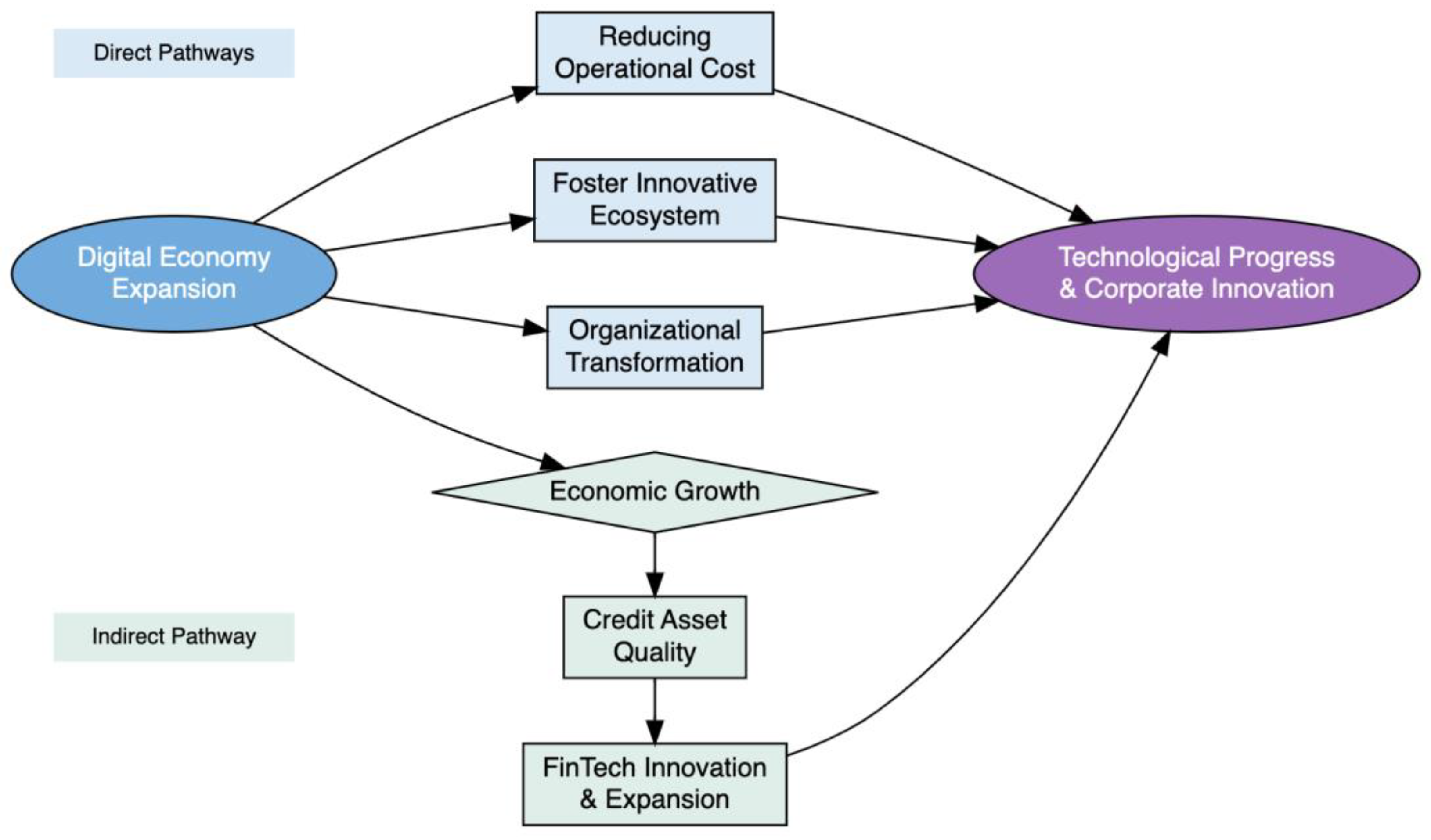
Figure 2.
Moran's I values over time by variable. The color gradient reflects the intensity of the Moran's I values, from low (blue) to high (red).Shapes of data points indicate the statistical significance of Moran's I statistic. Round points represent years with non-significant spatial autocorrelation (p > 0.05), while triangular points denote years with significant spatial autocorrelation (p ≤ 0.05).
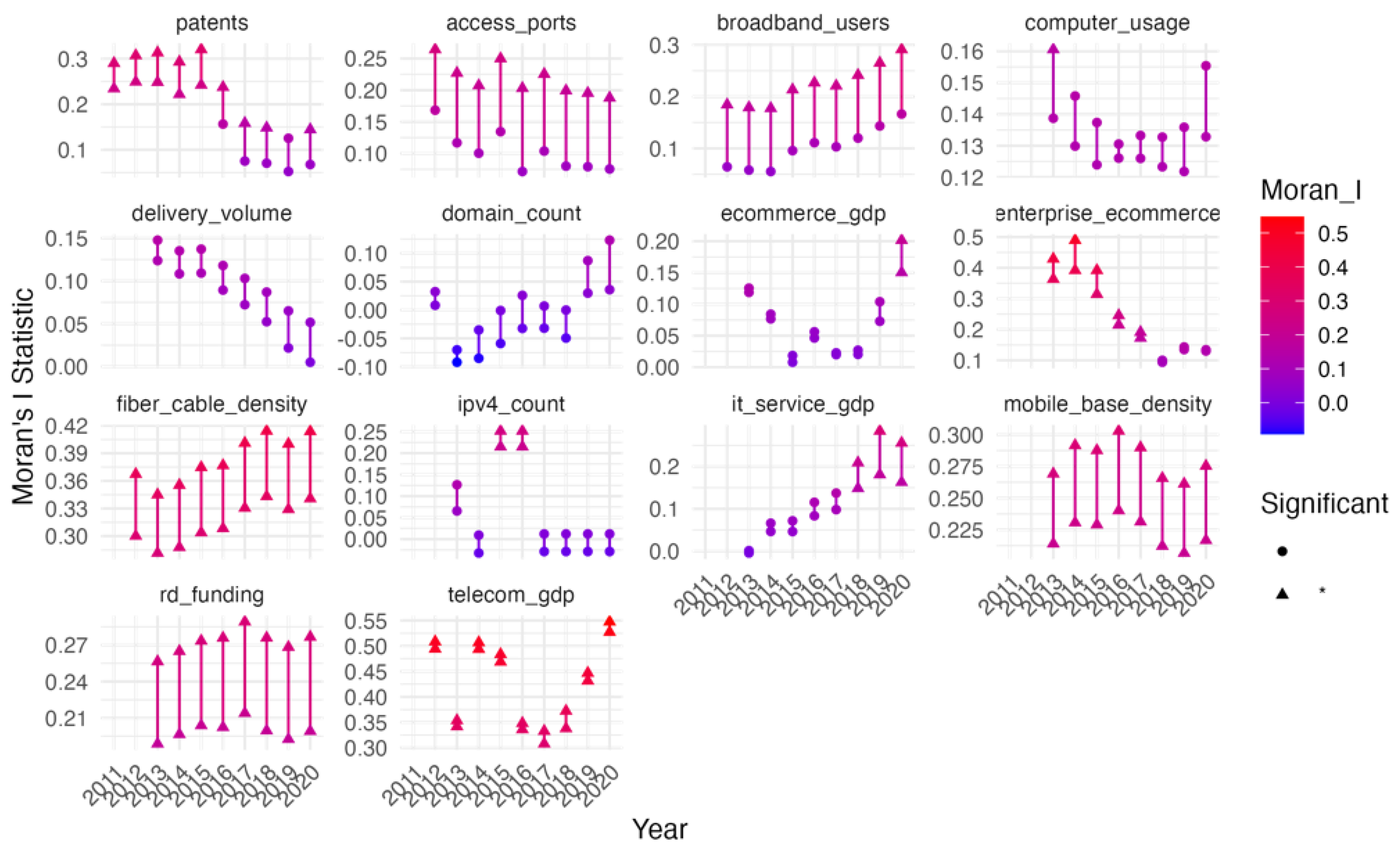
Figure 3.
Comparison of model performance metrics for test samples using normalized values of RMSE, MAE, MdAPE, and inverse R². Lower values indicate better performance. The 'Average Index' represents the mean of all normalized metrics.
Figure 3.
Comparison of model performance metrics for test samples using normalized values of RMSE, MAE, MdAPE, and inverse R². Lower values indicate better performance. The 'Average Index' represents the mean of all normalized metrics.
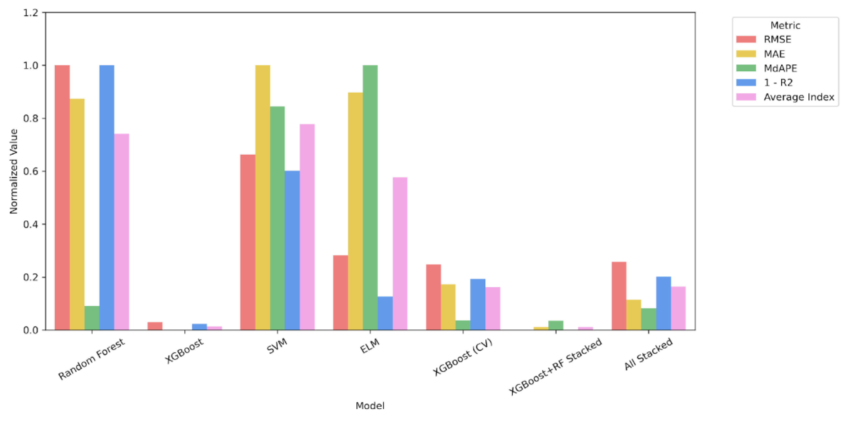
Figure 4.
Comparison of actual vs. predicted patent values across machine learning models: (a) Random Forest, (b) Extreme Learning Machine (ELM), (c) Support Vector Machine (SVM), (d) XGBoost, (e) RF & XGBoost combined, and (f) the final Stacked Model. The blue line represents the targeted R&D investment values, while the red line represents the predicted R&D values for the test dataset in each model.
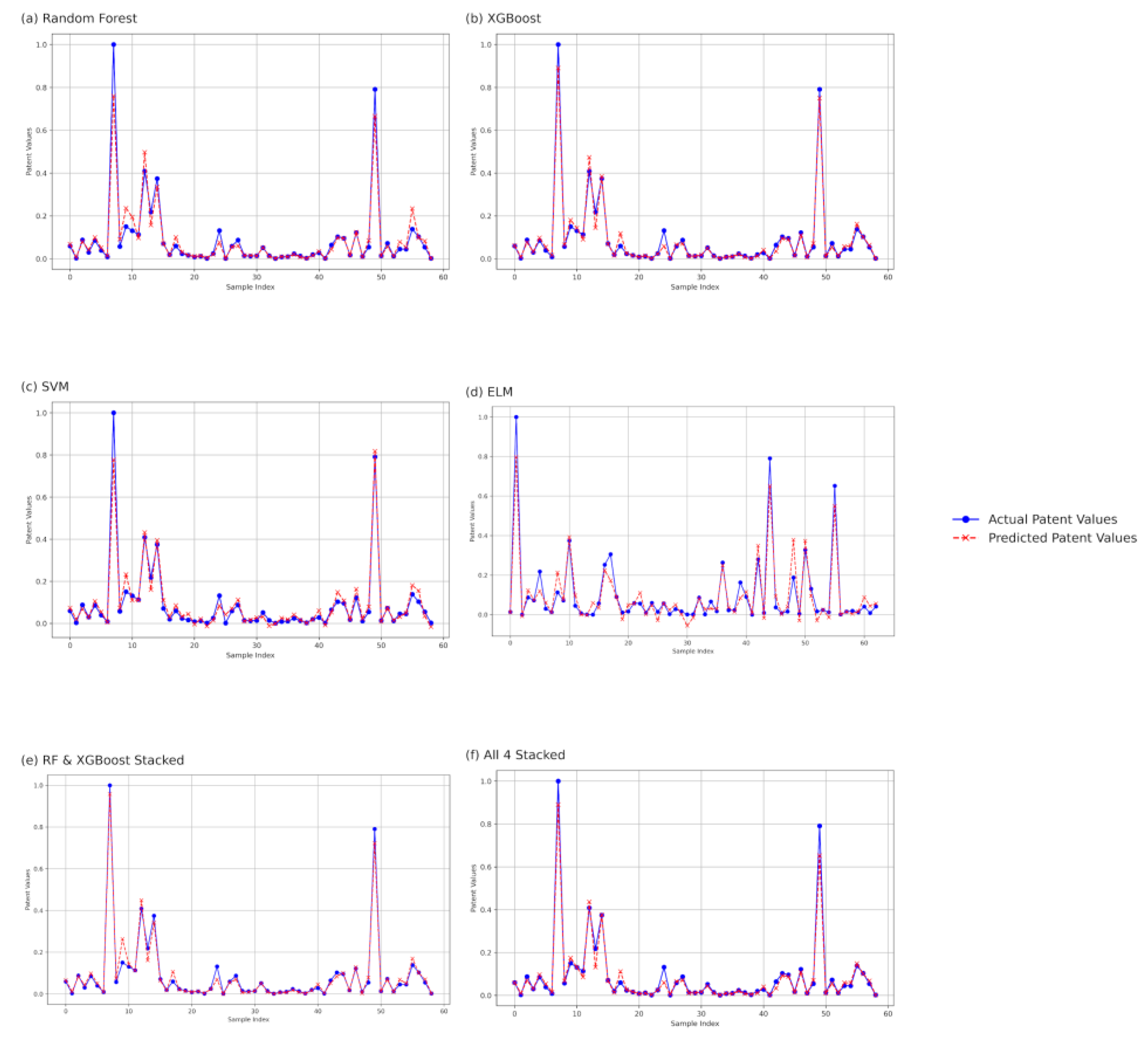

Table 1.
Digital economy variables and classification by layers.
| Layer | Variable | Variable Abbreviation | Reason for Classification |
|---|---|---|---|
| Core Layer | IPv4 Address Count | ipv4_count | IPv4 addresses are fundamental to internet infrastructure, aligning with IT consulting and telecommunications. |
| Internet Domain Count | domain_count | Internet domains are essential for online services and software-driven activities. | |
| Broadband Internet Users | broadband_users | Broadband access is critical infrastructure for IT services, telecommunications, and digital operations. | |
| Internet Access Ports | access_ports | Internet access ports support foundational IT infrastructure and digital industrial content. | |
| Long-Distance Fiber Optic Cable Length per Unit Area | fiber_cable_density | Fiber optic cables are the backbone of telecommunications and digital industrial services. | |
| Mobile Base Station Density | mobile_base_density | Mobile base stations are critical infrastructure for telecommunications and IT services. | |
| IT Service Revenue as Percentage of GDP | it_service_gdp | IT services, including software development and consulting, are central to the core digital economy. | |
| Telecom Services Revenue as Percentage of GDP | telecom_gdp | Telecom services form a foundational part of the digital industrial content in the core layer. | |
| Broad Layer | E-commerce Revenue as Percentage of GDP | ecommerce_gdp | E-commerce aligns with the broad layer as a key component of digital trade and algorithmic economic activities. |
| Express Delivery Volume | delivery_volume | Express delivery supports the e-commerce ecosystem, which is part of the broad layer. | |
| Proportion of Enterprises Engaged in E-commerce | enterprise_ecommerce | E-commerce enterprise participation is part of the broad layer, supporting the digital trade economy. | |
| Narrow Layer | R&D Funding | rd_funding | R&D funding drives digital services, platform innovations, and advancements in the digital economy. |
| Number of Computers Used per 100 Employees | computer_usage | Computer usage supports the platform economy and digital services by enabling productivity tools and platforms. |
Table 2.
Characteristics of common error metrics in model evaluation.
| Metric | Interpretation | Sensitivity to Outliers | Unit Dependence |
|---|---|---|---|
| RMSE | Penalizes large errors | High | Same as target variable |
| MAPE | Median percentage-based error | Moderate | Unitless |
| MAE | Average absolute error | Low | Same as target variable |
Table 3.
Moran's I and Geary's for patents and digital economic predictors over 2011- 2020. Proportion Significant represents the fraction of years in which the variable showed significant spatial autocorrelation (p < 0.05). It is calculated as (Significant Years / Total Years).
Table 3.
Moran's I and Geary's for patents and digital economic predictors over 2011- 2020. Proportion Significant represents the fraction of years in which the variable showed significant spatial autocorrelation (p < 0.05). It is calculated as (Significant Years / Total Years).
| Variable | Weight Type | Moran's Mean | Moran's P-Value | Moran's Significant Years | Moran's Total Years | Moran's Proportion Significant | Geary's Mean | Geary's P-Value | Geary's Significant Years | Geary's Total Years | Geary's Proportion Significant |
|---|---|---|---|---|---|---|---|---|---|---|---|
| access_ports | Binary | 0.211909 | 2.70E-02 | 8 | 8 | 1 | 0.792435 | 0.103647 | 1 | 8 | 0.125 |
| access_ports | Row-standardized | 0.095211 | 1.73E-01 | 0 | 8 | 0 | 0.943141 | 0.348676 | 0 | 8 | 0 |
| broadband_users | Binary | 0.226952 | 2.26E-02 | 8 | 8 | 1 | 0.778581 | 0.093397 | 1 | 8 | 0.125 |
| broadband_users | Row-standardized | 0.106632 | 1.57E-01 | 0 | 8 | 0 | 0.934157 | 0.330132 | 0 | 8 | 0 |
| computer_usage | Binary | 0.127828 | 7.62E-02 | 0 | 8 | 0 | 0.566018 | 0.028701 | 8 | 8 | 1 |
| computer_usage | Row-standardized | 0.141443 | 7.30E-02 | 1 | 8 | 0.125 | 0.695284 | 0.028113 | 8 | 8 | 1 |
| delivery_volume | Binary | 0.105563 | 1.09E-01 | 0 | 8 | 0 | 0.752825 | 0.157597 | 0 | 8 | 0 |
| delivery_volume | Row-standardized | 0.072743 | 1.93E-01 | 0 | 8 | 0 | 1.016883 | 0.537215 | 0 | 8 | 0 |
| domain_count | Binary | 0.017021 | 3.54E-01 | 0 | 8 | 0 | 0.788724 | 0.213897 | 1 | 8 | 0.125 |
| domain_count | Row-standardized | -0.03557 | 5.12E-01 | 0 | 8 | 0 | 0.975974 | 0.446764 | 0 | 8 | 0 |
| ecommerce_gdp | Binary | 0.064524 | 2.05E-01 | 1 | 8 | 0.125 | 0.590345 | 0.048219 | 5 | 8 | 0.625 |
| ecommerce_gdp | Row-standardized | 0.079589 | 1.93E-01 | 1 | 8 | 0.125 | 0.755151 | 0.078031 | 2 | 8 | 0.25 |
| enterprise_ecommerce | Binary | 0.227441 | 4.68E-02 | 5 | 8 | 0.625 | 0.564358 | 0.020763 | 6 | 8 | 0.75 |
| enterprise_ecommerce | Row-standardized | 0.264951 | 4.86E-02 | 5 | 8 | 0.625 | 0.640183 | 0.027061 | 6 | 8 | 0.75 |
| fiber_cable_density | Binary | 0.315709 | 1.11E-05 | 8 | 8 | 1 | 0.339695 | 0.019099 | 8 | 8 | 1 |
| fiber_cable_density | Row-standardized | 0.385109 | 5.96E-07 | 8 | 8 | 1 | 0.435242 | 0.00133 | 8 | 8 | 1 |
| ipv4_count | Binary | 0.085914 | 1.93E-01 | 2 | 8 | 0.25 | 0.635364 | 0.095414 | 2 | 8 | 0.25 |
| ipv4_count | Row-standardized | 0.043446 | 3.34E-01 | 2 | 8 | 0.25 | 0.885228 | 0.260824 | 0 | 8 | 0 |
| it_service_gdp | Binary | 0.096039 | 1.50E-01 | 3 | 8 | 0.375 | 0.619787 | 0.066267 | 3 | 8 | 0.375 |
| it_service_gdp | Row-standardized | 0.141866 | 1.23E-01 | 3 | 8 | 0.375 | 0.722599 | 0.072284 | 4 | 8 | 0.5 |
| mobile_base_density | Binary | 0.222615 | 4.16E-03 | 8 | 8 | 1 | 0.41174 | 0.017976 | 8 | 8 | 1 |
| mobile_base_density | Row-standardized | 0.280395 | 1.11E-03 | 8 | 8 | 1 | 0.532612 | 0.003765 | 8 | 8 | 1 |
| patents | Binary | 0.217555 | 2.51E-02 | 7 | 8 | 0.875 | 0.736945 | 0.136887 | 1 | 8 | 0.125 |
| patents | Row-standardized | 0.141918 | 1.06E-01 | 3 | 8 | 0.375 | 0.974252 | 0.445514 | 0 | 8 | 0 |
| rd_funding | Binary | 0.27263 | 5.11E-03 | 8 | 8 | 1 | 0.744202 | 0.104182 | 0 | 8 | 0 |
| rd_funding | Row-standardized | 0.199609 | 3.31E-02 | 8 | 8 | 1 | 0.869696 | 0.196437 | 0 | 8 | 0 |
| telecom_gdp | Binary | 0.412085 | 9.78E-04 | 8 | 8 | 1 | 0.512501 | 0.002287 | 8 | 8 | 1 |
| telecom_gdp | Row-standardized | 0.417459 | 1.41E-03 | 8 | 8 | 1 | 0.532877 | 0.00165 | 8 | 8 | 1 |
Table 4.
Machine Learning model parameters.
| Model | Tuning Applied | Base Models | Meta-Learner | Hyperparameters (Tuned / Applied) |
|---|---|---|---|---|
| XGBoost | Default | N/A | N/A | n_estimators=100, max_depth=6, learning_rate=0.1, subsample=1, colsample_bytree=1, objective='reg:squarederror' |
| Random Forest | Default | N/A | N/A | n_estimators=100, max_depth=6, random_state=42 |
| SVM | Tuned | N/A | N/A | kernel='rbf'; GridSearchCV tuning for C, gamma |
| Meta-Model (XGBoost) | Tuned | N/A | N/A | GridSearchCV tuning for learning_rate, n_estimators, max_depth, subsample, colsample_bytree |
| Stacked Model (Full Ensemble) | N/A | XGBoost, RF, SVM, ELM | XGBoost | |
| XGBoost: objective='reg:squarederror', n_estimators=100, max_depth=6 | ||||
| RF: n_estimators=100, max_depth=6, random_state=42 | ||||
| SVM: kernel='rbf' | ||||
| ELM: n_hidden=1000 | ||||
| Stacked Model (RF + XGBoost) | N/A | XGBoost, RF | Linear Regression | |
| XGBoost: booster='gbtree', learning_rate=0.2, n_estimators=300, max_depth=6, subsample=0.8, colsample_bytree=1.0, objective='reg:squarederror' | ||||
| RF: n_estimators=300, max_depth=6, min_samples_split=2, min_samples_leaf=1, random_state=42 | ||||
Table 5.
Performance metrics of base models and stacked models.
| Model | Sample Size | RMSE | MAE | MdAPE (%) | R² | t-Value | p-Value |
|---|---|---|---|---|---|---|---|
| Random Forest - Training | 136 | 0.0194 | 0.01 | 10.28 | 0.9838 | 0.3392 | 0.735 |
| Random Forest - Testing | 59 | 0.0449 | 0.0212 | 18.9 | 0.9309 | 0.1251 | 0.9008 |
| XGBoost - Training | 136 | 0.0006 | 0.0004 | 0.56 | 1 | 0 | 1 |
| XGBoost - Testing | 59 | 0.0253 | 0.0136 | 16.84 | 0.978 | 0.6143 | 0.5414 |
| SVM - Training | 136 | 0.0088 | 0.0076 | 12.3 | 0.9966 | 0.0574 | 0.9543 |
| SVM - Testing | 59 | 0.0381 | 0.0223 | 36.01 | 0.9501 | 0.1805 | 0.8574 |
| ELM - Training | 136 | 0.0249 | 0.0194 | 33.42 | 0.9683 | -0.0002 | 0.9999 |
| ELM - Testing | 59 | 0.0304 | 0.0214 | 39.56 | 0.973 | -0.2136 | 0.8316 |
| XGBoost - Training (CV) | 136 | 0.0005 | 0.0004 | 0.64 | 1 | -0.0008 | 0.9994 |
| XGBoost - Testing (CV) | 59 | 0.0297 | 0.0151 | 17.65 | 0.9698 | -0.1971 | 0.8444 |
| XGBoost-RF Stacked Model - Training | 136 | 0.0127 | 0.0067 | 5.41 | 0.993 | 0.4404 | 0.6603 |
| XGBoost-RF Stacked Model - Testing | 59 | 0.0247 | 0.0137 | 17.62 | 0.9791 | 0.0171 | 0.9864 |
| 4-Model Stacked - Training | 136 | 0.0007 | 0.0005 | 0.6538 | 1 | 0 | 1 |
| 4-Model Stacked - Testing | 59 | 0.0299 | 0.0146 | 18.7018 | 0.9694 | 1.5252 | 0.1327 |
Disclaimer/Publisher’s Note: The statements, opinions and data contained in all publications are solely those of the individual author(s) and contributor(s) and not of MDPI and/or the editor(s). MDPI and/or the editor(s) disclaim responsibility for any injury to people or property resulting from any ideas, methods, instructions or products referred to in the content. |
© 2025 by the authors. Licensee MDPI, Basel, Switzerland. This article is an open access article distributed under the terms and conditions of the Creative Commons Attribution (CC BY) license (http://creativecommons.org/licenses/by/4.0/).
Copyright: This open access article is published under a Creative Commons CC BY 4.0 license, which permit the free download, distribution, and reuse, provided that the author and preprint are cited in any reuse.


