
Submitted:
14 May 2025
Posted:
15 May 2025
You are already at the latest version
Abstract
Plant variety/genotype identification has many applications in establishing the identity of plants including protection of intellectual property rights. The variety may be important for operational reasons based on field performance or post-harvest processing. Genome sequencing methods have improved and become more feasible for use, making examination of the whole genome, which provides all possible information on the genotype, the ultimate way to distinguish plant varieties. Here, we present a standard protocol that could be used to identify a genotype of any plant species of interest from whole genome sequence data. The method was tested by application to the distinction of 41 varieties of tetraploid blueberry (Vaccinium Corymbosum L.). Using minimum mapping-coverage threshold, stringent variant filters and accurately identifying and excluding data-noise resulted in the generation of high confidence homozygous SNP uniquely shared between an unknown and a reference for utility in variety identification. The approach used aimed to minimize the impact of sequencing errors and coincident sequencing of only one allele of any heterozygous base. Adoption of a standard protocol and the establishment of sequence databases for all varieties of important plant species will be required to provide reliable variety identification in critical industrial or legal applications.
Keywords:
plant genotyping
; whole genome sequencing
; variety identification
1. Introduction
Plant variety identification is central to the protection /preservation of plant varieties and the policing of the intellectual property rights of plant breeders [1]. Plant variety identification may also be important in the marketing of agricultural and food products and the testing of the purity of foods [2]. Biosecurity and food safety issues may also require the determination of the varietal identity of plants. Plant genotyping has been conducted using a range of molecular tools that measure specific genetic loci [3,4]. Plant species have been widely distinguished by analysis of ribosomal genes [5]. Early genotype/variety-specific makers were based upon arbitrary primer PCR methods, microsatellite or short sequence repeat (SSR) analysis [6]. Single nucleotide polymorphism (SNP) represents a nucleotide change at a specific position in the genome sequence [7,8]. Advances in DNA sequencing methods have resulted in the widespread use of SNP analysis in plant identification [9,10]. Many techniques for SNP discovery have been used [4,11,12,13,14,15,16]. However, improvements in DNA sequencing technology have resulted in a convergence of DNA sequencing and genotyping approaches [2,15]. SNP analysis of the entire plant genome sequence enables the distinction of genotypes that vary by as little as a single nucleotide. Next generation sequencing allows detection of point mutations in plants that may be associated with useful phenotypes. Continuing advances in DNA sequencing have made the sequencing of the whole genome increasingly more cost effective [4,15,17,18].
Here, using short read sequence data from 41 blueberry varieties, we present a standard protocol for routine high-confidence SNP variant-based identification of plants for use in the distinction of plant varieties.
2. Materials and Methods
2.1. Leaf Sample Collection
A total of fifty-seven sample collections, S01 to S57, (Table S1) of leaf tissue, each consisting of 20 to 25 leaves, were made from field-grown plants of 41 blueberry varieties (S01 to S40 and S45) at Mountain Blue Orchards, Tabulam NSW 2469, Australia. Leaf samples, collections S01 to S39, S40, S45 and S50, were used as Reference samples for variety identification analysis. Additionally, to determine variation in “variant analysis” and factors affecting it, leaf sample collections S40 to S57, from the two varieties Masena and Eureka, were used in replicate analysis comprising technical and biological replicates. Technical replicate analysis was based upon one technical replicate library (Tec-rep) preparation from each of five replicate leaf collections from the same plant (P1L1 to P1L5) and labelled as “/P1/L1 to P1/L5” each for the variety Masena with library #s B40 to B44 and Eureka with library #s B45 to B49. Biological replicate analysis was conducted for three biological-replicate library (Bio1, Bio2 and Bio3) preparations, where each of the library preparations was prepared from replicate leaf collections one each from five plants (P1L1 to P5L1) and labelled as “/P1/L1/” to “/P5/L1/” each for the variety Masena with Bio1 library consisting of B40, B50 to B53, Bio2 consisting of B58 to B62, and Bio3 consisting of B68 to B72 and for Eureka with Bio1 library consisting of B45, B54 to B57, Bio2 consisting of B63 to B67 and Bio3 consisting of B73 to B77 (Table S1).
After harvesting, leaf samples were immediately secured in labelled perforated cellophane bags, within 2 minutes snap-frozen in the field by emersion in liquid nitrogen and then transferred covered with dry-ice for the duration of transport until storage in a -80oC freezer in the laboratory. Frozen leaf samples stored at -80℃ were first coarse pulverized under liquid nitrogen using a mortar and pestle and either stored at -80℃ or the containers containing the powder were placed on dry ice and then finely pulverized under cryogenic conditions. For fine pulverization, the coarsely ground leaf samples, contained in jars placed on dry ice, were transferred into a liquid-nitrogen-cooled steel canister with a steel ball, ensuring no liquid nitrogen is contained in the steel canisters, and then finely pulverized (25 frequency for 1 minute) using a Tissue Lyser II (Qiagen, USA). The finely ground leaf powder was stored at -80℃ until ready for DNA extraction.
2.2. Structuring of Samples for Varietal, Technical and Biological Library Preparation
Labelling of leaf sample #s with corresponding identification #s for genotype (G), blueberry library (B), plant (P) and leaf (L) and overall sample codes (Table S1), is explained as follows. Leaf samples S01 to S39 was treated as Reference (Ref) samples for variety analysis, their sequencing libraries labelled as B01 to B39 respectively, and their overall sample codes identified as “G#/S#B#/P1/L1/Ref-rep#1”. DNA extracted from Masena leaf sample S40 and Eureka leaf sample S45 was used correspondingly as Reference for variety analysis, as technical replicates and biological replicates set1 for “Variability in SNP Variant Analysis”, their corresponding sequencing libraries labelled as B40 and B45 respectively and their overall sample codes identified as “G#/S#/B#/P1/L1/Ref/Tec-rep1/Bio1-rep1”. For variety analysis, samples S01 to S39, S45 (Eureka) and S50 (Masena) were treated as variety Reference and sample S40 (Masena) was treated as the Unknown (Unk) variety.
DNA extracted from leaf samples S40 to S44 and S45 to S49 was used as technical replicates for “Variability in SNP Variant Analysis”, their corresponding sequencing libraries labelled as B40 to B44 and B45 to B49 respectively, and their overall sample codes labelled as “G#/S#/B#/P1/L#/Tec-rep#”. DNA extracted from leaf samples S50 to S57 was used as biological replicates set 1 for “Variability in SNP Variant Analysis”, their corresponding sequencing libraries labelled as B50 to B57 respectively, and their overall sample codes identified as “G#/S#/B#/P#/L1/Bio1-rep#”.
The same DNA extracted from leaf samples S40 and S45 of the variety Masena which was used for variety analysis and also as technical replicates and biological replicates set1, was also used as biological replicates set 2 and set 3 for “Variability in SNP Variant Analysis”, with their sequencing libraries labelled as B58, B63 and B68, B73 respectively, and their sample codes identified as “G#/S#/B#/P#/L1/Bio2-rep#” and “/G#/S#/B#/P#/L1/Bio3-rep#”, respectively. Similarly, the same DNA extracted from leaf samples S50 to S57 used as biological replicates set-1, was also used as biological replicates set-2 and as biological replicates set-3 with their corresponding sequencing libraries labelled as B59 to B62, B64 to B67 and B69 to B72, B74 to B77 respectively, and their overall sample codes identified as “G#/S#/B#/P#/L1/Bio2-rep#” and “G#/S#/B#/P#/L1/Bio3-rep#” respectively.
Libraries corresponding to samples used as Reference, Reference/technical replicate/biological replicate set1, technical replicate, biological replicate set-1 and biological replicate set-2 were sequenced in one lane while those corresponding to biological replicate set-3 were sequenced in a separate lane.
2.3. DNA Extraction
The finely ground leaf samples were subjected to DNA extraction using an established method [19]. Isolated DNA was dissolved in 100 µl of 10 mM Tris-HCL buffer pH 8.0. DNA quality was assessed by measuring the absorbance ratios (A260/A280 optimal is 1.9 to 2.0 and A260/A230 optimal is over 2.0) and absorbance profile using the Nanodrop Spectrophotometer (ThermoFisher Scientific, USA). The isolated DNA was resolved on a gel to assess the level of DNA breakage (shearing), with the DNA concentration and total amount assessed by comparing the brightness intensity of the resolved DNA to that of known amount of resolved lambda DNA.
2.4. DNA Sequencing and Sequence Data Output
The extracted genomic DNA of all samples, used for variety analysis and variability in SNP variant analysis, were subjected to the “Illumina DNA PCR-free Prep” indexed library preparation and then subjected to short read Illumina sequencing at 150 bp paired end (PE) reads on the Illumina NovaSeq X sequencing meachine (Illumina, San Diego, USA). Sixty-seven libraries, B01 to B67, corresponding to Reference, Reference/technical replicate/biological replicate set1, technical replicate, biological replicate set-1 and biological replicate set-2 samples were sequenced across six 10B lanes. Ten libraries, B68 to B77, corresponding to biological replicate set-3 samples were sequenced in one 10B lane. With sequence data (150bp PE reads) output range of 375 Gb/10B lane, the expected raw sequence data yield per sample of above 33 Gb is equivalent to a coverage of above 55 times (X) of the blueberry monoploid genome size of 600 Mb.
2.5. Data Analysis
All data analysis was undertaken using the CLC Genomics Workbench software 24.0.1 (Qiagen, USA).
2.6. Raw Sequence Data Processing and Data Output
Raw sequence data (150 bp PE reads) was trimmed for quality scores at quality limit of 0.01 resulting in over 99% of the trimmed data having an average PHRED score of over 34. Other parameters for trimming were, trim ambiguous nucleotides is “Yes”; read-through adaptor trimming is “Yes”; discard reads with length is “<50 and >1000 bases”.
2.7. Stage-M1: Optimisation of Read Mapping Parameters
In Stage-M1, the optimal combination of read length fraction (LF) and read similarity fraction (SF), both basic mapping parameters, was identified. The tool “Map Reads to Reference” was used to map PE trimmed Illumina reads to the diploid blueberry genome sequence (Vaccinium darrowii) as a reference sequence. A read mapping titration was undertaken, involving four combinations of read length fraction/similarity fraction mapping parameters settings from the most to least stringent: 1.0/0.95, 1.0/0.9, 0.9/0.9, and 0.8/0.8. Read mapping parameters not changed were, Masking mode is “No”; Mismatch score is “1”; Mismatch cost is “2”; insertion cost is “3”; deletion cost is “3”; non-specific match handling is “map randomly”; Execution mode is “Standard” and Minimum seed length is “15”. Genome sequence of Vaccinium darrowii (600Mb genome size) was downloaded from NCBI on 19/10/2023 (GenBank GCA_020921065.1, USDA_Vadar_1.0_pri_genomic, Yu et al 2921). This analysis was applied to five blueberry varieties (S01/B01 to S05/B05) to check if the results showed a similar trend, and if yes would obviate the need to subject the read mapping titration to all samples.
2.8. Stage-M2: Use of Optimized Read Mapping Parameters and Correction of Mapped Reads
Stage-M2 involved using the optimized mapping length fraction and similarity fraction parameters (identified from Stage-M1) and mapping the PE trimmed reads of each of the blueberry samples to the reference genome sequence followed by four sequential steps (Step-1 to Step-4), using as many analysis tools, to correct and improve the mapping of the reads mapped at Stage-M1. Stage-M2-Step-1 involved using the tool “Remove Duplicate Mapped Reads” to remove any duplicate reads in the read mapping file which can cause false inflation of the variant frequency leading to inaccurate zygosity of the variant calls. Stage-M2-Step-2 involved using the tool “Extract Reads” to remove broken reads mapped in the mapping file while retaining the PE mapped reads. Mapped broken pairs reads can map to incorrect location on the reference genome sequence and may contribute to erroneous variant calls. Stage-M2-Step-3 involved using the tool “InDels and Structural Variants” to identify and list erroneously generated structural variants covering insertions, deletions, inversions and tandem duplications in read mappings. Erroneously mapped reads can lead to erroneously generated structural variant calls which in turn can cause erroneous variant calls. Hence, this step identifies erroneously generated structural variants which can be used to correct the mapping file from the preceding step. Stage-M2-Step-4 involved using the tool “Local Realignment” to correct the read mapping file from Stage-M2-Step-2 at locations corresponding to the listed erroneously generated structural variants identified at Stage-M2-Step-3. The process involves the use of the structural variants identified in Stage-M2-Step-3 as a guide to locally realign the read mapped in the read mapping file from Stage-M2-Step-2 to generate a corrected read mapping file referred to as Locally Realigned (LR-) read mapping file. This LR-read mapping file is the one used to identify variants with respect to the reference genome sequence.
2.9. Stage-V1: Optimisation of Variant Detection Parameters
In Stage-V1, the optimal combination of variant (allele) detection parameters, “Minimum Frequency” (MF) and “Minimum Count” (MC) of the variant allele, was identified. A variant detection titration was undertaken to detect variants, where the LR-read mapping files (Stage-M2-Step-4) were subjected to the tool “Fixed Ploidy Variant” (FPV) detection involving six combinations of MF/MC parameters, 50/5, 35/4, 30/3, 25/3, 20/3 and 15/3. Variant allele detection parameters not changed were, Ploidy is “2” (to detect hyper allelic variants), Required variant probability (%) is “90.0”, Ignore positions with coverage above is “100,000”, Ignore broken pairs is “Yes”, Ignore non-specific matches is “Reads”, Minimum mapped reads coverage is “10”, Base quality filter is “Yes” (with settings within include: Neighborhood radius is “5”, Minimum central quality is “20”, Minimum neighborhood quality is “15”) and Read direction filter is “Yes” (with settings within include: Direction frequency (%) is “5.0”), Relative read direction filter is “Yes” (with settings within include Significance (%) is “1.0”) and Read position filter is “Yes” (with Significance % is “1.0”). The variants identified were filtered to identify homozygous single nucleotide polymorphisms (Hom-SNPs) and heterozygous SNPs (Het-SNPs). Filter parameters for Hom-SNPs were, Type is “SNVs”, reference allele contains is “No”, Zygosity is “Homozygous”, Read coverage is “≥ 20”, allele frequency is “100%”. Filter parameters for Het-SNPs were, Type is “SNVs”, reference allele contains “No”, Zygosity is “Heterozygous”, allele frequency is “≥ selected allele frequency and ≤ (100 – selected allele frequency)”. Hence, Stage-V1 involved determining the optimal FPV detection parameters to maximise the detection of Hom-SNPs and Het-SNPs followed by selecting those which are high confidence SNP variants. This analysis was applied to the LR-read mapping file of the same five blueberry varieties (S01/B01 to S05/B05), generated at Stage-M1, to check if the variants identified showed a similar trend across the five blueberry varieties, thus obviating the need to subject the FPV titration to all samples.
2.10. Stage-V2: Use of Optimized Variant Detection Parameters on All Samples
Stage-V2 involved applying the optimized FPV detection MF and MC parameter to all blueberry samples trimmed sequence files to identify Hom-SNPs and Het-SNPs. Variant allele detection parameters not changed were the same as used in Stage-V1. The variants identified were filtered to identify Hom-SNPs at minimum read coverage of 20 and allele frequency of 100% as outlined in Stage-V1. The variants identified were also filtered to identify Het-SNPs.
2.11. Stage-V3: Paired Variant Comparison Analysis with the Unknown and a Reference Sample
The blueberry sequence data file and the Hom-SNPs file of Masena B40, corresponding to leaf sample collection S40, sample library B40 and overall sample code of Masena/G10/S40/B40/P1/L1/ Ref-rep#1/Tec-rep#1/Bio1-rep#1 (Table S1), was treated as the Unknown (Unk) for the Paired Variant Comparison (PVC) analysis. The Hom-SNPs files of all other blueberry samples, corresponding to library #s B01 to B39 and B45 were treated as Reference samples. The blueberry variety Masena used as a Reference sample corresponded to leaf sample collection S-50, sample library B50 and overall sample code Masena/G10/S50/B50/P2/L1/ Bio1-rep#2 (Table S1).
At this stage, the Paired Variant Comparison analysis was undertaken pairwise using a pair of Hom-SNPs files involving the Hom-SNPs file of the Unknown blueberry (Masena B40) and the Hom-SNPs file of each of the blueberry Reference samples. The Paired Variant Comparison analysis involved two steps. At Stage-V3-Step-1, the tool “Identify Shared Variants” was used to combine the Hom-SNPs of the Unknown and a Reference sample, at a frequency threshold = 0, (the Unknown and a Reference sample) generating a Hom-SNPs-(Unk&Ref-B# PVC)-file of the Unknown and the specific Reference sample used. At Stage-V3-Step-2, the Hom-SNPs-(Unk&Ref-B# PVC)-file, was subjected to a filtering process to identify Hom-SNPs that are Common (shared) and Hom-SNPs that are Not-common (not shared) between the pair of samples. All the Not-common Hom-SNPs should be unique Hom-SNPs as they are identified by the variant identification process (Stage V2) to be present in the mapped reads of one sample and not the other of the sample pair. However, several mapping scenarios including the deficiency of mapped reads with desired depth, mis-mapped reads, etc, may suggest that the Not-common Hom-SNPs are not all unique (Unique?) but instead consists of a mixture of Truly Unique (True-Unique) Hom-SNPs and those which are Not-Truly Unique which we refer to henceforth as Data noise (Data-noise) Hom-SNPs. From any of the Hom-SNPs-(Unk&Ref-B# PVC)-file, the Common (shared) Hom-SNPs were identified using the filters: Sample count is “2”, and the resulting file named as Com-Hom-SNPs-(Unk&Ref-B# PVC)-File. Likewise, From any of the Hom-SNPs-(Unk&Ref-B# PVC)-file, the Not-common Hom-SNPs in each of the two samples, the Unknown and the Reference sample used, were identified using the filters: Sample count is “1”, frequency is “100”, and the Origin Tracks contain is “-40” for the Unknown sample and the B# used for the Reference sample used. The resulting files with the Not-common-Hom-SNPs are named as, (Unk)-Unique?=True-Unique&Data-noise-Hom-SNPs-(Unk&Ref-B# PVC)-File and the (Ref-B#)-Unique?=True-Unique&Data-nnoise-Hom-SNPs-(Unk&Ref-B# PVC)-File, respectively.
2.12. Stage-V4: Subclassification of Not-Common (Unique?) Hom-SNPs Post PVC-Analysis
Actual mapping scenarios can be envisaged leading to the possibility that the Not-common Hom-SNPs are not-all-Unique (Unique?), as they can contain both True-Unique and Data-noise Hom-SNPs (Unique?=True-Unique&Data-noise Hom-SNPs). Two of the mapping scenarios lead to the identification of the True-Unique Hom-SNPs while three of the mapping scenarios lead to the identification of the Data-noise Hom-SNPs. Hence, the Not-common Hom-SNPs in the Unique?=True-Unique+Data-noise-Hom-SNPs-(Unk&Ref-B# PVC)-File and in the (Ref-B)-Unique?=True-Unique+Data-noise-Hom-SNPs-(Unk&Ref-B# PVC)-File, were interrogated for the five possible mapping scenarios to explain why the Not-common Hom-SNPs are called in one sample and absent in the other and how many of these are True-Unique Hom-SNPs and Data-noise Hom-SNPs.
The Not-common Hom-SNPs file of the Unknown and the corresponding LR mapping file of the Reference sample, and vice versa, were analysed to define the nature and counts of nucleotides in the mapped reads at positions corresponding to each of the Not-common Hom-SNPs. This analysis is aimed to subclassify the Not-common Hom-SNPs into five sub-classes, corresponding to each of the of the five possible mapping scenarios. The five subclasses of the mapping scenarios leading to identification of the Not-common also referred to as Unique? Hom-SNPs fall within two groups, corresponding to the “Data-noise” and the “TrueUnique” Hom-SNPs. The Data-noise-Hom-SNPs are comprised of three subclasses of mapping scenarios abbreviated as Data-noise(*C), Data-noise(S1) and Data-noise(S2). The TrueUnique Hom-SNPs are comprised of two subclasses of mapping scenarios abbreviated as True-Unique(U1) and True-Unique(U2). Abbreviation definitions with respect to mapping scenarios are: Unique?=Data-noise(*C), the variant is not a Unique Hom-SNP as the same Hom-SNP is also present in the other sample but this variant is not called by the variant caller as the mapped read depth is ≥ 20 but failure of other variant quality filters; Unique?=Data-noise(S1), spuriously called as Unique Hom-SNPs type1 as the same Hom-SNP is also present in the other sample and hence is probably a common Hom-SNP, but this variant is not called by the variant caller, due to failure of mapped reads depth and other variant quality filters or only of the variant quality filters; Unique?=True-Unique(U1), True-Unique type1 as the variant is also homozygous in the other sample but this variant is not called by the variant caller as it is the same as the nucleotide allele present in the genome reference sequence; Unique?= TrueUnique(U2), True-Unique type 2 as variant is a Het-SNP in the other sample which is filtered away while selecting only for the Hom-SNPs; Unique?= Data-noise(S2) indicating spuriously called Hom-SNPs type2, involving a couple of scenarios, one where although the mapped reads satisfy the read mapping depth and all variant quality filters, the variant called in the other sample is filtered away due to the variant call linked with indels, and the other where there are no reads mapped resulting in no variant calls made by the variant caller.
At this stage, the tool “Identify Known Mutations from Mapping” was conducted separately for two pairs of input files, consisting of the Not-common Hom-SNPs file of one sample (example Unknown B40) and the LR mapping file of the other sample (example Reference sample B45) and vice versa. The “Identify Known Mutations from Mapping” was undertaken using the settings: Detection frequency % is “50.0”, create summarized overview track is “Yes”, create individual variant tracks is “Yes”, ignore broken pairs is “Yes”, ignore non-specific matches is “Yes”, and include partially covering reads is “No”. The outcome of this analysis, for each pair of input files, are two files each: the “Summarized Overview File” (file name corresponds to file name of the input Hom-SNPs variant file) and the “Individual Variant Track file” (file name corresponds to the input name of the LR mapping file). The two “Individual Variant Track file” files, one each of the Unknown and the Reference sample, were subjected to filtering processes to identify the six subclasses of the Not-common or Unique? Hom-SNPs.
Filters used: for the subclass Data-noise(*C) are undertaken in two steps: In Stage-V4-Data-noise-Step1, using filter: MFAA frequency is “<= 10”, results in intermediate-Stage-V4-Data-noise-Step1*C file. Step2: Take the intermediate-Stage-V4-Data-noise-Step1*C file and using the filter: Coverage is “>= 20”, results in the Data-noise(*C)-Hom-SNPs-(Unk&Ref PVC)-File which contains the Hom-SNPs of subclass Data-noise(*C). To identify Unique? Hom-SNPs of subclass Data-noise(S1), the tool “Filter against known variants” was used to deduct the subclass Data-noise(*C) Hom-SNPs present in the Data-noise(*C)-Hom-SNPs-(Unk&Ref PVC)-File, from the Hom-SNPs in the intermediate-Stage-V4-Data-noise-Step1*C file.
Filters used: for the subclass True-Unique(U1) are: MFAA frequency is “>= 90”, Coverage is “>= 20”, and Most frequent alternative allele (MFAA) doesn't contain “-“. Filters used: for subclass True-Unique(U2) are: MFAA frequency is “>10”, MFAA frequency is “<90”, Coverage is “>=10”, MFAA count is “>= 3”, and Most frequent alternative allele (MFAA) doesn't contain “-“.
To identify Hom-SNPs in subclass Data-noise(S2), use the tool “Identify Shared Variants” at Frequency threshold is “0” to combine the Hom-SNPs of class “Ture-Unique(U1)” and “True-Unique(U2)”. Use the tool “Filter against known variants” to deduct the Hom-SNPs present in two files, with subclass True-Unique(U1) and True-Unique(U2) and the Hom-SNPs in the intermediate-Stage-V4-Data-noise-Step1*C file, from the Hom-SNPs in the “Individual Variant Track file”.
From this analysis, the number of Hom-SNPs within each subclass is obtained for both the Not-common Hom-SNPs sample files used for the PVC-analysis. Once identified, the Unique? Hom-SNPs of each subclass from both the files were added together.
2.13. Stage-V5: Combining PVC Hom-SNPs Files of All Unknown & Reference Pairs and Filtering to Remove Data-Noise
At this Stage, a combined-PVC Hom-SNPs file is generated without or after filtering out the data-noise.
The PVC-analysis derived Hom-SNPs files from each sample pair, the Unknown and each of the forty-one Reference samples (the Unknown Blueberry B40 is common), were combined using the tool “Identify Shared Variants” at Frequency threshold = zero, ensuring the Hom-SNPs across all the sample pairs are included. The resulting file is labelled as Hom-SNPs-combined-41-Ref (all-Unk&Ref PVC)-File or in short “File-A (Combined Hom-SNPs)”. Although this file can be used to identify uniquely shared Hom-SNPs between the Unknown and any other of the Reference samples used, this file contains Data-noise and Persisting-Data-noise which when filtered and its implication on the accuracy of variety identification is explained below.
The Unique? Hom-SNPs from the PVC-analysis of each pair of Unk&Ref (Unknown is common), contains data-noise of sub-classes Data-noise(*C), Data-noise(S1) and Data-noise(S2)”. The PVC and Mutation-analysis generated Hom-SNPs files corresponding to Data-noise between the Unknown and each of the forty-one Reference samples were combined to obtain the file labelled as Hom-SNPs-Data-noise(*C&S1&S2)-in-combined-41-Ref (all-Unk&Ref PVC)-File or in short “File-B (Combined Hom-SNPs Data-noise)”. The Unique? Hom-SNPs of subclasses True-Unique(U1) and True-Unique(U2), derived from the PVC-analysis of the same varieties (Unknown is same variety as the Reference sample) are not True-Unique(U1 and U2) but are also data-Noise thus named Persisting-Data-noise of sub-classes False-Unique(F1) and & False-Unique(F2). The PVC and Mutation-analysis generated Hom-SNPs files corresponding to Persisting-Data-noise between the Unknown (Masena B40) and the closest Reference sample match) were combined to obtain the file labelled as Hom-SNPs-Persisting-Data-noise(F1&F2)-in-combined-41-Ref (all-Unk&Ref PVC)-File or in short “File-C (Combined Hom-SNPs Persisting-Data-noise)”.
The File-A (Combined Hom-SNPs) (containing data-noise) was filtered to remove only the Hom-SNPs corresponding to data-noise subclasses, Data-noise(*C), Data-noise(S1) and Data-noise(S2) present in the file File-B (Combined Hom-SNPs Data-noise) to generate the file labelled as File-A (Combined Hom-SNPs)-minus-File-B(Data-noise:*C,S1&S2) or in short File-A (Combined Hom-SNPs)-minus-File-B (Combined Hom-SNPs Data-noise) where File B contains Data-noise:*C,S1&S2.
The File-A (Combined Hom-SNPs) (containing data-noise) was also filtered to remove all the data-noise comprising of the Data-noise (*C, S1 & S2) and also the Persisting-Data-noise comprising of False-Unique(F1& F2) to generate the file labelled as File-A (Combined Hom-SNPs)-minus-File-B (Combined Hom-SNPs Data-noise) containing the Data-noise:*C,S1&S2)-minus-File-C (Combined Hom-SNPs Persisting-Data-noise) or in short File-A (Combined Hom-SNPs)-minus-(Data-noise:*C,S1&S2)-minus (Persisting-Data-noise: F1&F2).
2.14. Stage-V6: Variety identification Using the Combined-PVC Hom-SNPs with/Without Data-Noise
The variety identification process was applied to all three combined Hom-SNPs-Combined-PVC files generated in Stage-V5, “File-A (Combined Hom-SNPs)” or to File-A (Combined Hom-SNPs)-minus-File-B(Data-noise:*C,S1&S2) or to the File-A (Combined Hom-SNPs)-minus-File-B(Data-noise:*C,S1&S2)-minus- File-C (Combined Hom-SNPs Persisting-Data-noise:F1&F2) (Figure 3). The Variety identification protocol, “Protocol 1”, outlines the method development for variety identification including the concept around identifying the Data-noise and the Persistent-data-noise leading to variety identification. Variety Identification, “Alternate Protocol 2” and “Alternate Protocol 3”, may also be implemented to confirm the same outcome as obtained from Variety Identification: “Protocol 1” towards variety identification (Figure 3 and Figure S13).
The analysis relies on identifying Hom-SNPs uniquely shared between the Unknown sample Masena B40 and any other Reference sample. For example, uniquely shared Hom-SNPs between the Unknown sample (Masena B40) and the Masena Reference sample (B50) can be obtained by using the filters: Sample count is “2”, Origin Tracks contains “-40”, and Origin Tracks contains “-50”.
3. Results
3.1. DNA Quality
The purity of the DNA, assessed by examining the absorbance ratios at A260/230 and A260/230 (Table S2), was found to be within the acceptable range for all but a few samples. DNA fragmentation assessed by resolving the DNA on an agarose gel indicated the DNA to be mainly of high molecular weight (Figure S1). These quality metrics were acceptable for all the DNA samples as they were successfully sequenced on the Illumina sequencing platform to generate 150 bp paired end reads.
3.2. Consideration of Genome Coverage for Detecting High Confidence Homozygous SNPs
A heterozygous SNP (Het-SNP) position represented by two different nucleotides at a position can be identified by a variant caller at read depth as low as two and where both nucleotides are represented (assuming no errors in sequencing). However, the sequencing of DNA/library fragments with these alleles is random and where a small number of DNA/library fragments are available to be sequenced the same allele can by chance be sampled for sequencing each time leading to a false assessment of homozygosity (Table 1). This means that a Het-SNP position can be erroneously called a Homozygous SNP (Hom-SNP) where one of the two nucleotides is represented in all reads (assuming no errors in sequencing). A higher read depth results in a lower probability of repeatedly sequencing the same allele and leads to higher confidence variant calls. A high read mapping depth was used to increase the probability of correctly identifying a Het-SNP and consequently not erroneously identifying it to be a Hom-SNP.
Identification of high confidence Hom-SNP calls relies on increasing the read mapping depth. At a read mapping depth of one, there is a 100% probability of erroneously identifying a Het-SNP as a Hom-SNP or a no-variant call made if the nucleotide allele is the same as in the reference genome sequence, which progressively reduces with increasing read mapping depth (Table 2). At read mapping depth of 2 reads or at 3 reads, the probability of erroneously identifying a Het-SNP as a Hom-SNP reduces to 33.3% and 14.3% respectively (Table 2). Increasing the mapping read depth to 15, ensures a near 100% probability of correctly identifying a Het-SNP with 31 Het-SNP incorrectly identified as Hom-SNPs / million Het-SNP sites (Table 3). Increasing the mapping read depth to 21, ensures an effective 100% probability of correctly identifying a Het-SNP and with less than one Het-SNP incorrectly identified as Hom-SNPs / million Het-SNP sites (Table 3). Conversely, a read mapping depth of 21, also ensures a 100% probability of correctly identifying a Hom-SNP. Based on this data, we sequenced the blueberry samples at a minimum expected raw data depth of 55X of the monoploid genome size of 600 Mb, equating to 33 Gb, to achieve a minimum read mapping depth of 20X.
3.3. Raw Sequence Data Quality and Size as Times Genome Size of 600 Mb
The quality of the raw sequence data was high with over 90% of the sequence reads having a Phred quality score of above 30 (Table S3). The sequence data size of all samples, based on genome size of 600 Mb (1X), obtained at a minimum of 32.4X (19.5 Gb) and a maximum of 83.84X (50.3 Gb) at an average of 52.7X (31.6 Gb), was above the expected data size of 33 Gb (55X) for most samples. Post trimming, more than 80% of the sequence data was recovered at an average Phred score of above 35 and was at a minimum of 26.8X (16.1 Gb) and a maximum of 70.8X (42.5 Gb) which for most samples is above the expected data size of 33 Gb (55X) for most samples. The data size of the paired end component of the trimmed data, important for variant calling, was at a minimum of 25.4X (15.2 Gb), a maximum of 67.62X (40.6 Gb) and at an average of 42.1X (25.3 Gb), which is above the minimum requirement of 20X (12 Gb) (Figure S2 and Table S3).
3.4. Optimal Read Mapping and Variant Calling Parameters
Titration of read mapping parameters, involving length and similarity fractions (LF and SF), including the implementation of additional mapping filters, indicated the LF and SF each at 0.9 to be the optimal settings (Figure S3, A to E and Table S4). The least number of PE reads mapped at 1.0 LF and 0.95 SF, the most stringent mapping parameter, increased sharply to 1.0 LF and 0.9 SF and then slightly at 0.9 LF and 0.9 SF. Further sharp increase at 0.8 LF and 0.8 SF may be due to reduced mapping stringency and the cross-mapping of reads from other genomic locations thereby leading to erroneous variants. Using the optimal mapping parameters of 0.9 LF and 0.9 SF, a titration of variant calling parameters of minimum allele read count and allele frequency threshold was undertaken at six settings. The number of Hom-SNPs identified was steady at all the settings (Figure S3, F to J). The number of Het-SNP identified, as expected were least at the combination of “minimum allele read count / allele frequency” threshold, of 5/50 and steadily increased till the setting of 3/20 and a small increase thereafter at the last setting of 3/15. Hence, the optimal settings of “minimum allele read count / allele frequency” threshold is 3/20 to identify the maximum number of Het-SNPs. Based on the above information, the optimal mapping setting of 0.9 each for LF and SF and 5/50 for minimum allele read count / allele frequency was selected to identify Hom-SNP variants.
3.5. Mapping Coverage at Optimal Read Mapping Settings
Utilizing the optimal mapping setting of 0.9 each for LF and SF, the average read mapping coverage excluding the regions with no mapped reads was found to be above the desired 20X for all the blueberry samples except three of the Reference samples and two samples used for replication analysis (Figure 1). The fraction of the reference genome sequence, with mapped reads was above 0.86 for all samples tested (Figure S4) indicating high coverage of the reference genome sequence with mapped PE reads.
3.6. Identification of Variants
Het-SNPs were identified at a minimum read mapping coverage of 10, minor and major allele frequence range of 20% to 80% respectively and at a minimum variant allele read count of 3. The number of Het-SNPs ranged between 4.8 and 6.9 million (Figure S5A) and was strongly correlated with the sequence data size used for the variant analysis (Figure S5B). Hom-SNPs were filtered at a minimum read coverage of 20, at 100% allele frequency and at a minimum-variant read count of 5. The number of Hom-SNPs ranged between 0.7 M and 2.1 M (Figure S5A) and strongly correlated with the sequence data size used for the variant analysis (Figure S5C). Results also indicate that increasing the sequence data size above 45X leads to diminishing returns in terms of sequencing cost versus aiming to capture as many or all the Het-SNPs or Hom-SNPs present in the blueberry genome of a specific sample (Figure S5B and S5C).
3.7. Variability in Hom-SNPs Identified Within Technical and Biological Replicate Samples
Two blueberry samples, Masena and Eureka, were selected for technical and biological replication analysis. Technical replicates, P1L1 to P1L5, were represented as DNA extracted from five leaf samples from a single plant (Table S1). Biological replicates, P1L1 to P5L1, corresponded to DNA extracted from five leaf samples where each leaf sample was from a different plant (Table S1). The same DNA sample was subjected to three biological libraries, where library 1 and Library 2 were sequenced in the same lane while library 3 was sequenced in a separate lane. To assess variation in Hom-SNPs between samples of a common library preparations, for each of the two samples for replication analysis, pairwise variant comparison (PVC) analysis for Hom-SNPs was undertaken between 10 pairs of the five technical library samples and likewise between the five samples each within the three biological libraries. Similarly, to assess variation in Hom-SNPs between samples of different library preparations, for each of the two samples for replication analysis , PVC-analysis for Hom-SNPs was undertaken between 5 pairs of the 5 samples each between the three biological libraries.
The PVC-analysis between all the Masena samples and between all the Eureka samples identified both Common Hom-SNPs and Not-common Hom-SNPs (Table 4). The Common Hom-SNPs for Masena and Eureka technical library replicates samples were as high as 78.6% and 75.6% respectively (Table 4, Figure S6A and Figure S7A), with an average of 73.6 ±SD 4.9 and 70.2 ±SD 4.1 respectively indicating low variation between each of the ten paired comparisons for both the samples (Table S5 and Table S6). In addition, the PVA analysis between the Masena technical replicate sample, Blueberry B41 and all other Masena technical replicate samples resulted in a consistently lower number of Common Hom-SNPs (Figure S6A) resulting possibly from mapped PE trimmed data size of under 20X (1X is 600 Mb) and a read mapping coverage under 25 (Figure 1).
The trimmed paired-end (PE) reads were mapped to the genome sequence of Vaccinium darrowii (NCBI, Yue et al 2021) with optimised mapping settings and pipeline to address mis-mapping of PE reads. The data size of the input PE reads for mapping shown as times (X) genome size of 600 Mb was lower than 20X for some samples used as reference samples and used as technical and biological replicates. However, the average read mapping coverage, excluding the regions with zero coverage, was above 20X for all samples except three of the Reference samples and two samples Masena/G10/S50/B59/P2/L1/Bio2-rep#2 and Masena/G10/S50/B69/P2/L1/Bio3-rep#2 used for replicate analysis. Two samples, within the technical replicate set, represented as yellow bars were used for variety analysis, technical replicate analysis and biological replicate analysis. Average read-mapped coverage from 20 is marked with a horizontal broken black line.
The Common Hom-SNPs for Masena and Eureka Biological Library 1 replicate samples were as high as 79.2% and 82.6% respectively (Table 4, Figure S6B and Figure S7B), with an average of 70.3 ±SD 4.1 and 65.6 ±SD 10.6 respectively indicating low variation between each of the ten comparisons for the Masena but not the Eureka samples (Table S5 and Table S6). The PVC-analysis between the Masena Biological library 1 sample Blueberry B52, to all other Masena library 1 replicate samples resulted consistently in low numbers of Common Hom-SNPs (Figure S6B) while for the Eureka sample it was Blueberry B57 (Figure S7B). Both the samples, Blueberry B52 and Blueberry B57 had mapped PE trimmed data size under 20X (1X is 600 Mb) and a read mapping coverage under and just above 20 respectively (Figure 1).
The Common Hom-SNPs for Masena and Eureka Biological Library 2 replicates samples were as high as 72.1% and 76.5% respectively (Table 4, Figure S6C and Figure S7C), with an average of 62.4 ±SD 5.8 and 67.5 ±SD 5.0 respectively indicating low variation between each of the ten comparisons for the Masena and the Eureka samples (Table S5 and Table S6). The PVC-analysis between the Masena Biological library 2 sample, Blueberry B59, to all other Masena library 2 replicate samples resulted consistently in low numbers of Common Hom-SNPs (Figure S6C) while for the Eureka sample set it was Blueberry B63 (Figure S7C). Both the samples, Blueberry B59 and Blueberry B63, had mapped PE trimmed data size under 20X (1X is 600 Mb) and a read mapping coverage under 20 and 25 respectively (Figure 1).
The Common Hom-SNPs for Masena and Eureka Biological Library 3 replicates samples were as high as 81.73% and 79.42% respectively (Table 4, Figure S6D and Figure S7D), with an average of 61.04 ±SD 18.86 and 72.47 ±SD 4.56 respectively indicating high variation between each of the ten PVC-analysis for the Masena samples but low for the Eureka samples (Table S5 and Table S6). The PVC-analysis between the Masena Biological library 3 sample, Blueberry B69, to all other Masena Biological library 3 replicate samples resulted consistently in low numbers of Common Hom-SNPs (Figure S6D) and this sample had mapped PE trimmed data size under 20X (1X is 600 Mb) and a read mapping coverage below 20 (Figure 1).
These results indicate that a mapped read data size below 20X (1X is 600 Mb) and specially read mapping depth below 20 can impact on maximizing the capture of SNP variants using NGS data. In a few of the samples used for replication analysis, the Hom-SNPs, at best ranging from 20% to 40% and worst at 60%, are captured as Not-common in the pairwise analysis of the same variety indicating not all the Hom-SNPs are captured consistently between the replicates (Table 4).
3.8. Variability in PVC-Analysis Generated Hom-SNPs Between Biological Replicates
Within each of the three biological libraries, each of the five Masena samples were compared pairwise for common Hom-SNPs, and likewise undertaken also for the Eureka samples biological libraries (Figure S6 E to G and Figure S7 E to G). For the Masena and Eureka samples, the Common Hom-SNPs from the PVC-analysis showed more variation for the samples within the biological replicate library 3 and biological replicate library 1, respectively, than from samples within the other two biological replicate libraries or from the technical replicate library (Table S5 and Table S6). Comparison of sample 1 to 5 for Common Hom-SNPs between biological libraries (Library 1, 2 and 3) for the Masena and Eureka sample set, showed more variation for Masena sample 3 and Eureka sample 4 (Table S5 and Table S6).
3.9. Common and Not-Common Hom-SNPs Between Masena and Between Masena and Eureka Samples
PVC-analysis between two of the same blueberry variety, Masena samples B40 and B50 (biological replicates), identified 70.5% as Common Hom-SNPs and 29.5% Not-common Hom-SNPs (Figure 2A). Similar results were obtained from the analysis between all the Masena samples (all 55 combinations of Masena sample B40 within technical replicates, within the biological replicates and between biological replicates) where 66.1% (average) were Common Hom-SNPs and 36.5% (average) Not-common Hom-SNPs (Figure S8). Likewise, similar results were also obtained from PVC-analysis between all the Eureka samples, (all 55 combinations of Eureka sample B45 within technical replicates, within the biological replicates and between biological replicates) where 68.6% were Common Hom-SNPs and 32.1% Not-common Hom-SNPs (Figure S8).
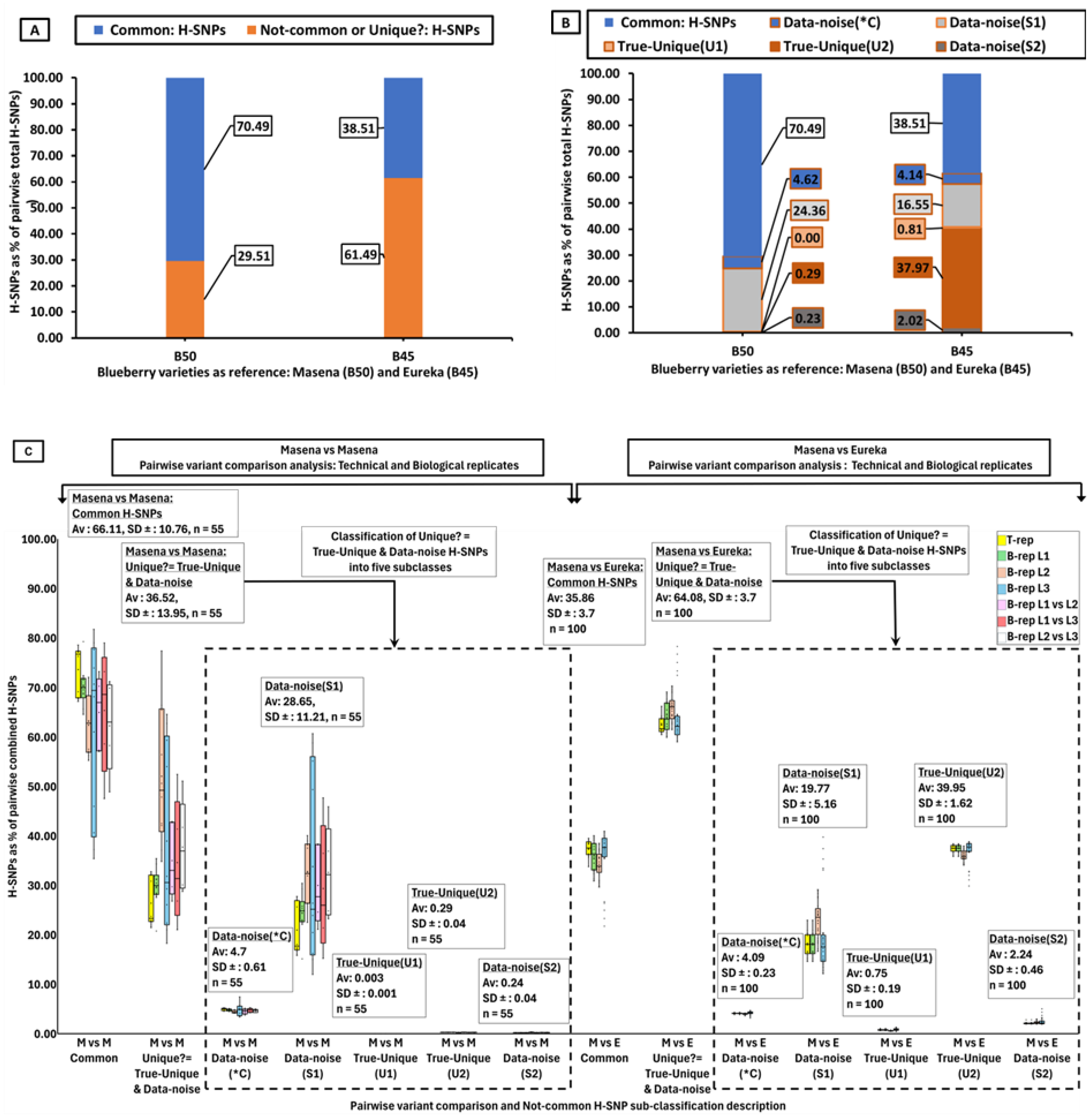
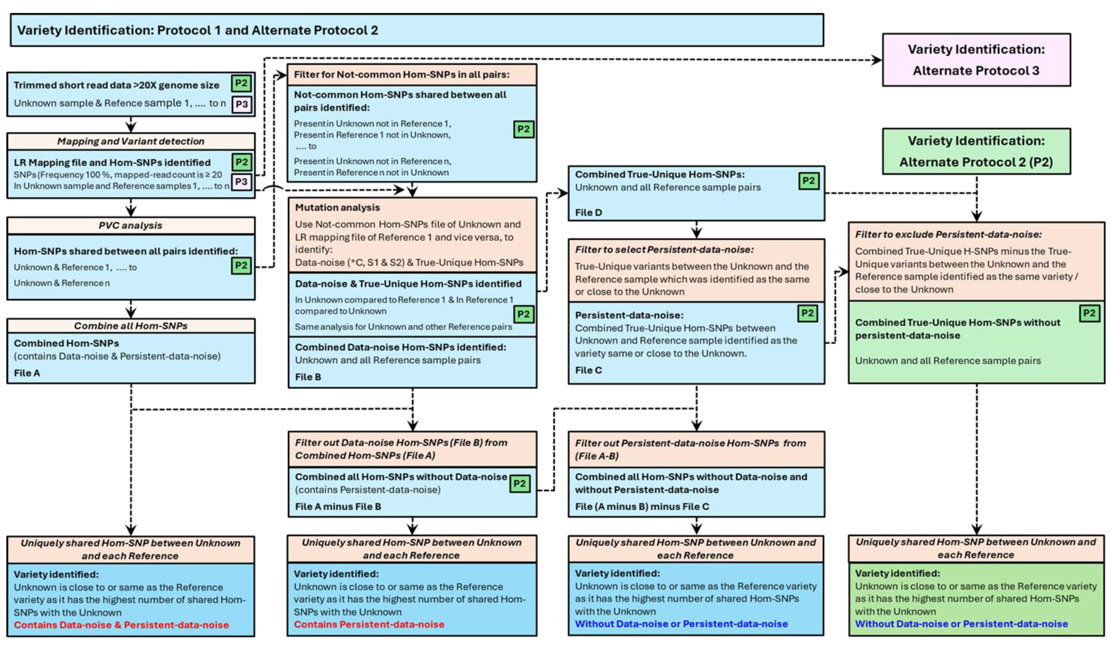
Figure 2.
PVC analysis between blueberry samples to identify Common, Not-common or Unique? and sub-classes of Not-common Hom-SNPs.
Figure 2.
PVC analysis between blueberry samples to identify Common, Not-common or Unique? and sub-classes of Not-common Hom-SNPs.
Figure 3.
Schematic of Variety Identification Protocol 1 and Alternate Protocol 2.
PVC-analysis between two different blueberry varieties, Masena sample B40 and Eureka sample B45 identified 38.5% as common Hom-SNPs and 61.5% Not-common Hom-SNPs (Figure 2A), and similar results were obtained between all the Masena and Eureka samples (all 100 combinations within technical replicates and within the biological replicates) where 35.9% (average) were common Hom-SNPs and 64.1% (average) non-common Hom-SNPs (Figure S8). Similar results were obtained from PVC-analysis between Masena B40 and each of the 39 different blueberry varieties, where 39.5% (average) were common Hom-SNPs and 60.5% (average) non-common Hom-SNPs (Figure S9).
The PVC-analysis results indicate the number of Common-Hom-SNPs were more when the pair of samples were the same variety (Masena vs Masena) while the Not-common-Hom-SNPs were more when the pair of samples were different varieties (Masena vs Eureka). In addition, the PVC-analysis successfully identified the Not-common or Unique Hom-SNPs between two different blueberry varieties, which can be informative SNPs for variety identification. However, the identification of Not-common or Unique Hom-SNPs between two samples that are the same variety indicates these Hom-SNPs must all be erroneous as they cannot be Unique but should all be Not-Unique between samples of the same variety. Hence, it is possible that the Not-common Hom-SNPs identified between two samples that are different blueberry varieties may not all be Unique (Unique?) and may contain both “True-Unique” and “Not-Unique” Hom-SNPs”, the latter representing Data-noise. Identifying the two components of the Not-common or Unique? Hom-SNPs, the “True-Unique” and “Data-noise” (Not-Unique), and using only the True-Unique Hom-SNPs of the Not-common Hom-SNPs would be crucial in increasing the accuracy of variety identification.
PVC, pairwise variant comparison analysis between a pair of samples; H-SNPs/Hom-SNPs, homozygous single nucleotide polymorphism; Common Hom-SNPs, Hom-SNPs present in both samples; M, Masena sample; E, Eureka variety; Not-common or Unique?; Hom-SNPs present in one of the sample with no variant call in the other although implying to be unique with the possibility that some but not all to be unique (U?); Data-noise(*C), probably Common Hom-SNP as mapped at read depth ≥ 20 but failure of other variant quality filters, Data-noise(S1), spurious type1 due to failure of mapped reads depth or mapped read depth and other variant quality filters; True-Unique(U1), True unique type1 as variant is homozygous same as reference allele; True-Unique(U2), True unique type 2 as variant is heterozygous SNP; Data-noise(S2) indicating spurious type 2 (S2) due to the SNP call linked with indels or no reads mapped. As the Not-common or Unique? Hom-SNPs are not all unique and divided into two groups of five subclasses. The True-Unique group is comprised of two subclasses, the True-Unique(U1) and True-Unique(U2). The Data-noise group is comprised of three subclasses, the Data-noise(*C), Data-noise(S1) and Data-noise(S1). Hom-SNPs numbers indicated are a percentage of the total combined Hom-SNPs between a pair of samples taken for the PVC analysis. A, PVC analysis between the unknown sample (Masena B-40) and the Masena reference sample (B-50) and the Eureka reference sample (B45) showing the Common Hom-SNPS to be higher between the B-40 and B-50 PVC while the Not-common or Unique? Hom-SNPS to be higher between the B-40 and B-45. B, The major subclasses of Unique? Hom-SNPs are Data-noise (*C) and Data-noise(S1) for the Unknown (Masena) B-40 and Masena B-50 PVC comparison, and are Data-noise (*C) and Data-noise(S1) and True-Unique(U2) for the Unknown (Masena) B-40 and Eureka B-45 PVC comparison. C, Similar results as in B, were obtained from fifty-five PVC analyses between Masena vs Masena (technical and biological replicates) and from one-hundred PVC analyses between Masena vs Eureka including the subclasses of the Not-common or Unique? Hom-SNPs.
3.10. Sub-Classification of Not-Common Hom-SNPs Between the Same and Dissimilar Varieties
Identifying the “True-Unique” and “Data-noise” Hom-SNPs, the two components of the Not-common Hom-SNPs of the same variety, was undertaken by visual inspection of reads mapping at location corresponding to the Not-common or Unique? Hom-SNPs. This process led to the identification of read-mapping scenarios in one sample which led the variant caller in identifying the Hom-SNPs as Not-common in the other. Five read-mapping scenarios were identified leading to five subclasses of the Not-common or Unique? Hom-SNPs (Table 5), where three are grouped as “True-Unique” and two as “Data-noise” Hom-SNPs.
The True-Unique group, within the Not-common Hom-SNPs, is comprised of two subclasses, True-Unique(U1) and True-Unique(U2). The read-mapping scenario for subclass True-Unique(U1), is defined as, reads that are mapped and satisfy the defined read-depth and variant filter settings, but where the identified variant is a Hom-SNP and is the same nucleotide allele as in the reference genome sequence, the variant calling software does not record it as a variant. The read-mapping scenario for subclass True-Unique(U2), is defined as, reads that are mapped and satisfy the read-depth and variant filter settings, but the identified variant called is heterozygous and although recorded by the variant caller is filtered away when selecting only the Hom-SNPs. The Data-noise group, within the Not-common Hom-SNPs, is comprised of three subclasses, Data-noise(*C), Data-noise(S1) and Data-noise(S2). The read-mapping scenario for subclass Data-noise(*C), is defined as, the mapped reads have the same Hom-SNP as in the other sample, and satisfies the read-depth but not the variant filters settings resulting in the variant caller not recording the Hom-SNP variant. The read-mapping scenario for subclass Data-noise(S1), is defined as, the Hom-SNP is the same as in the other sample, reads are mapped but these either do not pass the variant filters or both the read depth and variant filters, resulting in no variant called by the variant caller. The mapping-scenario for the subclass Data-noise(S2), can be defined as, either, no reads are mapped at the corresponding location of the Hom-SNP resulting in the variant caller not recording a variant, or reads are mapped with the variant caller recording a multi nucleotide variant (which may not be reliable) or a heterozygous call involving a deletion (unreliable due to mis-mapped reads at a homopolymer region) and although recorded by the variant caller is filtered away when selecting only Hom-SNPs.
The Not-common or Unique? Hom-SNPs (29.51%) identified from the PVC-analysis between Masena vs Masena (Figure 2A), where the two varieties are the same, were classified into the five subclasses as outlined above (Figure 2B). All three subclasses of the Data-noise (*C, S1 & S2) Not-common Hom-SNPs are present with Data-noise(S1) (24.36%) and Data-noise(*C) (4.62%) as the first two major components. Of the True-Unique (U1 and U2) Not-common Hom-SNPs, no Hom-SNPs corresponded to subclass True-Unique(U1) but Hom-SNPs at 0.23% corresponded to subclass True-Unique(U2) equating to 2,300 True-Unique(U2) Hom-SNPs/million Hom-SNPs. Similar results were also obtained when the Not-common or Unique? Hom-SNPs (average 36.52%) identified from PVC-analysis of all the 55 combinations of Masena vs Masena (technical and biological libraries) were subclassified into its two components (Figure 2C). All three subclasses of the Data-noise (*C, S1 & S2) Not-common Hom-SNPs are present with Data-noise(S1) (average 28.65%) and Data-noise(*C) (average 4.7%) as the first two major components. Of the two subclasses comprising the True-Unique (U1 and U2) Not-common Hom-SNPs, both subclasses True-Unique(U1) (average 0.003%) and True-Unique(U2) (average 0.29%) were present and equating to 30 True-Unique(U1) Hom-SNPs and 2,900 True-Unique(U2) Hom-SNPs respectively per million Hom-SNPS (Figure 2C).
The Not-common or Unique? Hom-SNPs (61.49%) identified from the PVC-analysis between Masena vs Eureka (Figure 2A), where the two varieties which are different, , were classified into the five subclasses as outlined above (Figure 2B). All three subclasses of Data-noise (*C, S1 & S2) Not-common Hom-SNPs are present with Data-noise(S1) (16.55%) and Data-noise(*C) (4.14%) as the first two major components. Of the two subclasses comprising the True-Unique (U1 and U2) Not-common Hom-SNPs, both subclasses True-Unique(U1) (0.81%) and True-Unique(U2) (37.97%) were present with the latter the major component. Similar results were also obtained when the Not-common or Unique? Hom-SNPs (average 64.08%) identified from PVC-analysis from all the 100 combinations of Masena vs Eureka (technical and biological libraries) were subclassified into its two components (Figure 2C). All three subclasses of the Data-noise (*C, S1 & S2) Not-common Hom-SNPs are present with Data-noise(S1) (average 19.77%) and Data-noise(*C) (average 4.09%) Hom-SNPs the first two major components. Of the two subclasses comprising the True-Unique (U1 and U2) Not-common Hom-SNPs, both subclasses True-Unique (U1) (average 0.75%) and True-Unique(U2) (average 39.95%) Hom-SNPs were present (Figure 2C).
As with the subclasses obtained for the Not-common or Unique? Hom-SNPs for Masena vs Eureka comparison, where the two varieties were different(Figure 2B and C), similar results were obtained when the Masena sample was compared pairwise to all the other thirty-nine blueberry varieties (Figure S10). All three subclasses of the Data-noise (*C, S1 & S2) Not-common Hom-SNPs are present with Data-noise(S1) and Data-noise(*C) the first two major components. Of the two subclasses comprising the True-Unique (U1 and U2) Not-common Hom-SNPs, both subclasses True-Unique (U1) (average 0.75%) and True-Unique(U2) (average 39.95%) Hom-SNPs were present with the latter the major component (Figure 2C).
The Data-noise Not-common Hom-SNPs, comprising of the subclasses Data-noise(*C), Data-noise(S1) and Data-noise(S2), are the non-informative Hom-SNPs and were filtered out from the Not-common or unique? Hom-SNPs before using them for varietal identification.
3.11. Variety Identification After Removal of Data-Noise Hom-SNPs
Identification of an Unknown variety compared to a specific cohort of selected Reference samples, is based on identifying the Hom-SNPs that are uniquely shared pairwise between an Unknown sample and a specific Reference sample and not with any of the other Reference samples within the cohort of Reference samples used. The detailed process of variety identification. as explained below. involves several steps collectively referred to as Variety Identification: Protocol 1 (Figure 3), with alternate protocols referred to a Variety Identification: Alternate Protocol 2 (Figure 3) and Variety Identification: Alternate Protocol 3 (Figure S13) can be implemented to confirm results.
Hom-SNPs, Homozygous SNPs; X genome size, time genome size of 600 Mb; LR mapping, outcome of optimised read mapping to a reference genome sequence; PVC analysis, Paired Variant Analysis between a pair of samples. Schematics for two protocols schemas are presented. Combining Hom-SNPs between the Unknown and a Reference sample generates Hom-SNPs common to both samples and unique Hom-SNPs present in one sample but not the other. Combing the unique Hom-SNPs from all sample pairs (File A) can be processed to identify shared Hom-SNPs between the Unknown sample and each of the Reference sample. If the Unknown sample variety matches one of the Reference varieties, then this Unknown-Reference sample pair should be the only pair to share a set of Hom-SNPs which would be unique to this pair of Unknown-Reference samples. However, using File A, shared variants between the Unknown and each of the Reference sample are not unique as some are also found to be shared Hom-SNPs between the Unknown sample and another Reference sample. This indicates an anomaly due to data noise which we have identified as Data-noise and Persistent-data-noise. When the Data-noise is identified (File B) and deducted from File A, data noise is removed for most of the Unknown/Reference sample pair comparison. When the Persistent-data-noise is identified and removed, the data noise is completely removed leaving with one Unknown/Reference pair with uniquely shared Hom-SNPs implying the Reference in question to be the same as/close to the Unknown sample. An alternate protocol (Alternate Protocol 2) is also presented here leading to the same outcome. Alternate protocol 3 with the same outcome can be used but is not explained here.
We used a suite of forty-one blueberry Reference samples including a Masena Reference sample B50. PVC-analysis generated Hom-SNPs files, between the Unknown sample and each of the forty-one Reference samples, were combined to obtain the “File-A (Combined Hom-SNPs)”. The Hom-SNPs corresponding to the Data-noise (*C, S1 and S2) present within the Not-common or Unique? Hom-SNPs between the Unknown sample and each of the forty-one Reference samples were also combined to obtain the “File-B (Combined Hom-SNPs Data-noise)”. Filtering out the Hom-SNPs in File-B (Combined Hom-SNPs Data-noise from File-A (Combined Hom-SNPs) generated the File-A (Combined Hom-SNPs)-minus-File-B(Data-noise: *C, S1 & S2).
Using File-A (Combined Hom-SNPs) for identifying the Unknown sample variety, the Hom-SNPs shared uniquely between the Unknown (Masena B40) and each of the forty-one Reference samples indicated the highest (18,673) to be between the unknown (Masena B40) and the Masena Reference B50 (Figure S11). The next highest number of uniquely shared Hom-SNPs is 2,593 between the Unknown sample and the blueberry sample B18 (not Masena) and for most of the other Reference samples the uniquely shared Hom-SNPs are under 500. Although this result clearly identified the Unknown sample to be the variety Masena, the presence of uniquely shared Hom-SNPs between the Unknown (Masena B40) and the Reference samples other than the Masena Reference B50 is expectedly due to data noise as identified between the Unknown and all the forty one Reference samples used (Figure 2 and Figure S10) and represented in File-B (Combined Hom-SNPs Data-noise are not filtered out.
When the File-A (Combined Hom-SNPs) if first subjected to removal of the Data-noise represented in File-B (Combined Hom-SNPs Data-noise, and then used for identifying the Unknown sample variety, the Hom-SNPs shared uniquely between the Unknown (Masena B40) and each of the forty-one Reference samples indicated the highest (5,806) to be between the unknown (Masena B40) and the Masena Reference B50 (Figure 4A). This result also clearly identified the Unknown sample to be the variety Masena. All but five of the other forty Reference samples, had no uniquely shared Hom-SNPs with the Unknown (Masena B40) sample, with B08, B24, B33 and B34 samples had one and B27 sample had two uniquely shared Hom-SNPs. However, the presence of uniquely shared variants, although as high as two Hom-SNPS, indicates the presence of Persisting-Data-noise other than Data-noise Hom-SNPs captured in File-B (Combined Hom-SNPs Data-noise which were filtered out. The Persisting-Data-noise was also observed when the analysis was undertaken with only six Reference samples including the Masena Reference B50 and the Eureka Reference B45, albeit the Unknown was clearly identified to be the variety Masena with 77,281 uniquely shared Hom-SNPs (Figure 4A insert).
H-SNPs/Hom-SNPs, homozygous SNPs; Bio1; Biological replicate library1. Hom-SNPs of the Unknown sample (Masena/G10/S40/B40/P1/L1/Ref-rep#1/Tec-rep#1/Bio1-rep#1) was compared pairwise, using the Paired Variant Comparison (PVC) analysis, with the Hom-SNPs from each of the forty-one blueberry Reference samples (B01 to B39, B50 and B45) to obtain a Hom-SNPs-(Unk&Ref-B# PVC)-file, one for each of the forty-one Unknown and reference sample pair. A shared Hom-SNPs file was generated by combining the Hom-SNPs-(Unk&Ref-B# PVC)-files of all the forty-one unknown and reference pairs. Shared Hom-SNPs identified between the Unknown and each of the reference forty-one samples were then subjected to variety identification analysis where in A, Post removal of Data noise(*C, S1 and S2), 5,806 were the most uniquely shared Hom-SNPs between the Unknown sample (Masena, Bio1, plant1, B40) and the Masena reference sample (Plant2, Bio1, B50). In addition, between one or two Hom-SNPs were uniquely shared with five other reference samples. The presence of the uniquely shared Hom-SNPs between the unknown sample and with five other reference samples indicates the presence of another class of data-noise we refer to as Persisting-Data-noise. B, The Persisting-Data-noise referred to as subclass False-Unique(F1) and False-Unique(F2) was originally identified as True-Unique(U1 and U2) from the Unknown and Masena Reference (B-50) PVA comparison. Post removal of Data-noise(*C, S1 and S2) and the False-Unique (F1 and F2), the uniquely shared Hom-SNPs were found to be 5,806 between the Unknown sample (Masena, Bio1, plant1, B40) and the Masena reference sample (Plant2, Bio1, B50). Similar results were obtained when the analysis was undertaken with six reference blueberry varieties (figure-insert).
Identifying the nature of the Persistent-data-noise was important to its removal for variety identification with no data noise. On examining the read mapping and variant track files corresponding to the Reference samples B08, B24, B27, B33 and B34 with the Persisting-Data-noise (Figure 4A), we identified the cause of the Persisting-Data-noise to be due to the presence of erroneously called Hom-SNPs of the classes True-Unique(U1) and True-Unique(U2) in the Unknown (Masena B40) but correctly called as Het-SNPs in the Masena Reference B50 (Figure S12). The PVC-analysis between the Unknown (Masena B40) and the Masena Reference B50 (Figure 2B) sample would have erroneously identified a number of SNPs to be Hom-SNPs in the Unknown sample, leading to their inclusion as the Not-Common or Unique? Hom-SNPs of the sub-classes True-Unique(U1) and True-Unique(U2), thus leading to the Persisting-Data-noise. As expected, further filtering of the Persisting-Data-noise Hom-SNPs captured in File-C (Combined Hom-SNPs Persisting-Data-noise was undertaken from the file obtained by deducting the Data-noise captured in File-B (Combined Hom-SNPs Data-noise from File-A (Combined Hom-SNPs). Post filtering of the Persistent-data-noise indicated the highest number of uniquely shared Hom-SNPs (5,806) to be between the Unknown (Masena B40) and the Masena Reference sample B50 (Figure 4B) with zero uniquely shared Hom-SNPs between the Unknown and any of the other Reference samples. Similar results were obtained using the limited set of six Reference samples including the Masena Reference B50 and the Eureka Reference B45 (Figure 4B Insert).
4. Discussion
Variety identification is important in plant breeding, as it provides plant breeders a method to protect the variety generated thus providing benefits to growers and producers/funders of the breeding programs. A number of technologies based on variation present in the DNA have been used in plant identification [20] making use of single nucleotide polymorphisms (SNPs) [8,15,21]. Here, we present a protocol (Figure 3 and Figure S13), developed using commercial tetraploid blueberry (Vaccinium, spp.), using next generation sequencing (NGS) to identify SNPs and utilising Hom-SNPs to identify a plant variety compared to the Hom-SNPs of a set of Reference samples.
The accurate identification of a plant sample using SNPs from NGS, involves best practice procedures, starting from sample collection to sequence data analysis [22]. Care should be taken to source reliable plant material whose variety identity is known and hence can be used as Reference samples. Extracting DNA of good quality and of high molecular weight, critical for good quality NGS data, is dependent on using a workable DNA extraction protocol with the type of tissue which is easily accessible for harvest. The need to try several DNA extraction procedures with some modifications is not uncommon for recalcitrant species [23,24,25,26,27,28]. Once harvested, appropriate storage of the plant tissue immediately post-harvest, during travel and storage is important to maintain sample/DNA integrity. We harvested blueberry leaf material as the tissue type for DNA extraction. Leaves samples were immediately frozen under liquid nitrogen, kept frozen under dry-ice during transport and stored or processed under a -80C temperature regime. Using a standard CTAB-based method, large amounts of good quality high molecular weight DNA with no/low impurities was obtained and was successfully used for sequencing library preparation. The Illumina library kit, DNA Illumina DNA PCR-free Prep, was used to factor out any amplification bias causing the overrepresentation on one of the two alleles in mapped sequence reads at a Het-SNP location, thus avoiding the incorrect assigning of a Hom-SNP as a Het-SNP or vice versa.
SNPs between any two varieties are made up of Common SNPs and Not-common SNPs. Distinguishing two varieties depends on identifying and using the Not-common SNPs between the pair, which comprise of different types of Hom-SNP combinations (Hom-SNP vs Het-SNP, for example AA vs AT) or different Hom-SNP types (Hom-SNP vs Hom-SNP for example AA vs GG). Het-SNPs in both samples will be Common SNPs and so cannot be used to distinguish two varieties. However, it is important to ensure a Het-SNP is not erroneously called a Hom-SNP or conversely a Hom-SNP when called is a correct call. In the case of the outcrossing autotetraploid [29,30] blueberry samples used in this study, both the alleles of a Het-SNP should be equally represented with a 50% allele frequency or 50 mapped reads of each allele out of a total mapped-read depth coverage of 100. Assuming good quality sequence data is obtained, in practice, the equal representation of both the nucleotides of a Het-SNP bases in mapped reads is affected by the non-equal sampling of sister chromatids at various stages of the sample preparation including, DNA sampling, library preparation steps, sampling the library for sequencing and sequencing bias. The non-equal sampling will ultimately be exemplified in a disproportionate or the non-coincident representation of the Hom-SNP bases in the mapped sequence reads. Hence, the non-equal sampling can result in a dis-proportionate allele frequency of the Het-SNP, lower than the ideal 50%, and in some cases only one allele is represented at a 100% allele frequency leading to the Het-SNP variant being erroneously called as a Hom-SNP.
At a given Het-SNP position and read mapping coverage from 2 and above, there are only two instances of read mapping where all the reads have one or the other allele leading to two erroneous Hom-SNP calls. Increasing the read mapping coverage increases the instances of reads mapped with both alleles of a Het-SNP, thereby reducing the probability of an erroneous Hom-SNP call closer to zero. In sequencing a Het-SNP position using a collapsed reference genome sequence, the frequency of false calling it as a Hom-SNP, due to the dis-proportionate Het-SNP allele frequency, can be calculated (Table 2). For example, at a given Het-SNP position with read mapping depth of 2 and A/C alleles there are 4 possible variant call outcomes, mapped reads with either AA or CC alleles leading to Hom-SNP calls and AC or CA alleles leading to Het-SNPs calls. Consideration of mapped-read depth, critical for a high confidence call made at the beginning of the variant calling, resulted in computing the minimum mapped read depth of 20 required to reduce an erroneous Hom-SNP call close to zero (Table 2 and Table 3). Correctly identifying a heterozygous position relies on the sequencing reads with both alleles mapping at a specific location in its representative proportion, and this probability increases close to 100% at a specific read mapping depth. (Table 2 and Table 3). This demonstrates the need to have high coverage especially for large or heterozygous genomes even when the analysis is based only on homozygous variants (Table 1). As the blueberry cultivars we used are autotetraploids, the probability of all four nucleotide classes occurring at a position in the tetraploid genome is low, and as the reference genome sequence used is a diploid, the ~600 Mb monoploid blueberry genome size was used to calculate the required data size of 30X. Hence, samples were sequenced above 18 Gb and equivalent to a minimum of 30X the genome size of ~600 Mb monoploid blueberry genome [31], above the minimum mapped read depth requirement of 20 to account for some data loss at the raw sequence data trimming step. The sequence data yield obtained for the 77 blueberry samples post quality trim (0.01 quality trim, CLC Genomics), ranged from least data yield of 15.2 Gb (25.41 times genome size of 600 Mb) to highest data yield of 40.6 Gb (67.62 times genome size of 600 Mb) (Figure S2). For the Genotyping by Sequencing (GBS) method, a minimum read depth of 15 is suggested for polyploid species so as to be 95% sure that all four alleles are sequenced [32,33]. The dis-proportionate allele frequency of the Het-SNP also indicates the difficulty of identifying Het-SNP below the ideal 50% frequency, and the importance of undertaking a variant titration to define minimum allele frequency required for Het-Variant calling.
Trimmed data with more than the desired data size of 20X the 600 Mb genome size ensured the use of optimum data size (Figure S2) and the optimal mapping and variant detection parameters were determined using mapping and variant detection titration steps (Figure S3). The fraction of the reference genome sequence covered ranging from 0.86 to 0.91 and with the mapped read depth above 20X for most samples, ensured the sequence data size used is comparable between samples (Figure S4). Variability in SNPs identification caused by batch effects from tissue sampling replicates (comparing within Replicate Technical, Replicate Biological Library1 and Replicate Biological Library2 and Replicate Biological Library3), and sequencing library preparations (comparing Replicate Biological Library1 and Replicate Biological Library2 each with Replicate Biological Library3), was assessed by PVC-analysis between pairs of Masena samples or pairs of Eureka samples.
The varieties, Masena and Eureka were selected as Reference samples for the PVC-analysis to identify Hom-SNPs that are commonly shared (Common Hom-SNPs) and not-commonly shared (Not-common Hom-SNPs). Assuming every Hom-SNP is identified from PVC-analysis, when the two varieties are the same all the variants should be Common Hom-SNPs and none to be Not-common Hom-SNPs, while for varieties that are different the number of Common Hom-SNPs is expected to be lower than the Not-common Hom-SNPs which may be considered as unique SNPs. However, capturing all the Hom-SNPs in a sample is limited by the sequence data quality and read depth of the NGS data, accuracy of read mapping, and accuracy of the variant calling. Both Common and Not-Common Hom-SNPs were identified by PVC-analysis between Masena vs Masena, Eureka vs Eureka and Masena vs Eureka (Table S5 and Table S6 and Figures S6 and S7). The Common Hom-SNPs averaging 66.1% and 68.6% between Masena vs Masena and Eureka vs Eureka replicates, respectively, indicates some variability in the sequence data within these Reference samples (Table S1). Interestingly, the rest of the ~35% to ~36% of the Hom-SNPs must represent missing data as these were identified between the same Reference variety and hence cannot be considered as genuine Not-common or genuine Unique Hom-SNPs (Figure S8 and Table S5 and Table S6). PVC-analysis between Masena B40 and Masena B50, identified 29.51% missing data (Figure 2A) and ~35% (average) from all combinations between these two Reference samples, Masena and Eureka (Figure S8). Examining the read-mapping scenarios, the missing data was mainly of subclass Data-noise(*C) due to only failing the read mapped threshold of 20, or Data-noise(S1) due to also failing the variant quality filters, and Data-noise(S2) due to variants linked with InDels or no reads mapped (Figure 2B and C). Twenty-five percent of the Common Hom-SNPs between the Masena B40 vs Masena B50 PVC-analysis were identified at read-mapping depth between 20 to 30, while 72% were identified at read-mapping depth between 30 to 60. A small number of the Not-Common Hom-SNPs classified as True-Unique(U1) occurring due to the Hom-SNP same as the genomic reference genome sequence and True-Unique(U2) occurring due to erroneously calling a Het-SNP as a Hom-SNP, cannot be Unique Hom-SNPs between the same variety, and hence classified as False-Unique(F1) and False-Unique(F2). Not-Common Hom-SNPs at 61.49% were identified between the Reference samples Masena B40 vs Eureka B45 combination (Figure 2A) and ~64.1% (average) identified from all combinations between the Reference samples Masena and Eureka (Figure S8). These PVC-analysis identified Not-common or Unique? Hom-SNPs between Masena and Eureka, after sub-classification contained missing data corresponding to Data-noise (*C), Data-noise(S1) and Data-noise(S2) and also the genuinely or truly Unique Not-Common Hom-SNPs labelled as True-Unique(U1) and True-Unique(U2) (Figure 2B and 2C).
For varietal identification, the blueberry sample Masena B40 was treated as the Unknown sample and compared by PVC-analysis to each of the forty Reference blueberry samples including the Masena Reference sample B50 collected as a Biological Rep (Table S1). The Common Hom-SNPs and the Not-common Hom-SNPs were identified (Figure S9) and post combining the PVC-analysis derived Hom-SNPs variants of all Unknown/Reference pair combinations, the Unknown sample was identified to be the same or similar to the Masena Reference sample B50 with 18,673 uniquely shared Hom-SNPs (Figure S11). However, Hom-SNP variants uniquely shared between the Unknown and Reference samples other than the Masena Reference B50, are considered as Data-noise. The Data-noise identified is actually the missing-data present from the PVC-analysis between the Unknown sample and each of the Reference samples. Following the subclassified of the missing data into sub-classes, Data-noise(*C, S1 & S2) and the True-Unique(U1 & U2) (Figure S10) and removal of the Hom-SNPs corresponding to the Data-noise (*C, S1 & S2) reduced the number of instances of variants uniquely shared between the Unknown and Reference samples other than with the Masena Reference B50 (Figure 4A). However, even after filtering out the Data-noise, the occurrence of some instances of variants uniquely shared only between the Unknown and Reference samples other than with the Masena Reference B50, is also due to data noise of another class we label as Persisting-Data-noise (Figure 4A). Examining the read-mapping at location of the Hom-SNPs corresponding to the Persisting-Data-noise (Figure S12), indicated these to be the False-Unique Hom-SNPs between the Unknown sample and the Reference sample Masena Sample B50 (Figure 2B). Filtering out the False-Unique Hom-SNPs resulted in the complete elimination of data-noise and the only sample to have uniquely shared Hom-SNPs with the Unknown sample was the blueberry Reference sample Masena sample B50 (Figure 4B). The False-True-Unique Hom-SNPs are the Not-common Hom-SNPs between varieties which are the same, and these represent errors in variant calling where a Het-SNP is erroneously called a Hom-SNP even at coverage above 20. The “Variety identification Protocol 1" (Figure 3), outlines the method development process for variety identification including the concept around identifying the Data-noise and the Persistent-data-noise which needs to be removed for variety identification. Once developed, a shorter process for variety identification via “Variety identification Protocol 2” (Figure 3) or “Variety identification Protocol 3” can be implemented (Figure S13).
The missing data identified from all combinations between the Masena samples at 36.52% (average) (Figure 2C) is mainly due to areas of coverage under 20 which can occur at the PVC-analysis stage between any pair of samples and can be reduced by using sequence data with mapping coverage over 20 in these regions. Missing data at 25% was reported for genotyping by sequencing (GBS) approach in maize [34], which could be reduced to half or even lower using imputations approaches [34,35] but at the expense of increased genotyping error rate which was found to be 0.7% [36]. We identified an error rate of 0.29% identified as False-True-Unique Hom-SNPs identified from the PVC-analysis between 55 Masena sample combinations (Figure 2C). Kmer based heterozygosity was reported to be 1.27% [31]. Based on the heterozygosity between 0.85% to 1%, equating to 5.1 to 6.0 M Het-SNP sites in the blueberry genome (600 Mb), we estimate 17,400 of the Het-SNPs to be erroneously called as Hom-SNPs corresponding to a 0.29% error rate.
Prior to NGS, prevailing molecular marker technologies had limited use in understanding the genetic diversity in the blueberry group [37,38,39]. Microsatellite markers were used in a limited manner for genetic analysis of the various groups of blueberry [40]. The use GBS aided in identifying SNPs for genetic diversity and population structure analysis and phenological traits [33]. Microsatellite markers have also been used for genetic diversity analysis varietal identification, although requiring cumbersome non NGS approaches [41,42]. The protocol developed here (Figure 3 and Figure S13), is economical as the generated sequence data of the Reference samples can be reused and is also forward compatible as sequence data of additional Reference samples can be added to expand the sequence data of Reference sample cohort. The cost of SNP genotyping per data point using NGS has reduced [10,43] and thus utilising this approach is suited for variety identification. High throughput approaches using NGS sequencing and reduced representation approaches such as GBS [16,44,45] or SNP array-based approaches such as Axiom, Infinium, and MassARRAY iPLEX [17] are appropriate for screening large samples for genetic diversity and other genetic studies.
5. Conclusions
The SNPs data for the 41 blueberry samples should allow any blueberry variety within this cohort of blueberry samples to be identified. All varieties were easily associated with one of the genotypes in this group of varieties. Additional varieties can be added to expand the Reference sample cohort for the application of the technique to unknown samples that need to be considered. Use of this protocol to identify varieties in specific regions would need to include all know varieties from that region. The SNP data can also be used to identify variety-specific SNPs which are not present in any of the other blueberry varieties within this cohort of forty-one Reference samples. The variety-specific SNPs could be used to develop a cost-competitive assay test to identify blueberry varieties within a given cohort. This would be useful in the screening of larger numbers of samples in applications such as policing the sale of protected varieties on sale in a retail environment. The concept of identifying and removal of data-noise is not restricted to the use of the CLC Genomics Workbench and can be developed and applied using any software programs including command-line approaches. This approach should be useful for almost any plant species for which variety identification is required providing a robust genetic approach to variety identification in support of protection of biosecurity, food safety and intellectual property.
Supplementary Materials
The following supporting information can be downloaded at the website of this paper posted on Preprints.org, Figure S1: QC data for the extracted blueberry DNA; Figure S2: Short read paired end trimmed sequence read data for 77 Blueberry DNA samples; Figure S3: Titration analysis of mapping and SNP variant detection using of blueberry PE reads mapped to a reference genome; Figure S4: Fraction of the genome covered and average mapped coverage by paired end reads of blueberry samples; Figure S5: Heterozygous SNPs and homozygous SNPs across several blueberry samples with variable sequence data size; Figure S6: High confidence common homozygous SNPs between Eureka samples within technical and biological libraries and between different biological libraries; Figure S7: High confidence common homozygous SNPs between Eureka samples within technical and biological libraries and between different biological libraries; Figure S8: PVC-analysis between Massena and between Eureka blueberry samples to identify Common and Not-common Hom-SNPs; Figure S9: PVC-analysis between the unknown (Masena, B40) and forty blueberry varieties including Masena (B50) to identify Common and Not-Common Hom-SNPs; Figure S10: PVC-analysis and classification of the Not-common-Hom-SNPs between the unknown (Masena, B40) and forty-one blueberry varieties (B01 to B39, Masena B50 and Eureka B45); Figure S11: Identification of an Unknown blueberry sample using uniquely shared Hom-SNPs without filtering data-noise; Figure S12: Nature of the Persisting-data-noise in the variety identification analysis; Figure S13: Schematic of Variety Identification: Alternate Protocol 3; Table S1: Details of blueberry varieties/cultivars; Table S2: QC metrics of all 77 blueberry DNA samples; Table S3: QC of the sequence data of all blueberry samples; Table S4: Mapping titration of short read (Illumina @ 150bp paired end reads) of five blueberry varieties using V. darrowii genome sequence (Yu et.al. NCBI 2021) as the reference; Table S5: Statistical analysis of the percentage common Hom-SNPs from pairwise analysis for Masena technical and biological replicates; Table S6: Statistical analysis of common H-SNPs from pairwise analysis for Eureka technical and biological replicates.
Author Contributions
Conceptualization, AF, TG and RH.; data curation, AF.; lab, AF; methodology, AF and RH.; project administration, AF and RH; resources, RH and TG.; supervision, RH.; validation, AF.; visualization, AF.; writing—original draft, AF and RH.; writing, review and editing, AF, TG and RH. All authors read and agreed to the published version of the manuscript.
Funding
Samples of blueberry varieties were provided by Mountain Blue Orchards. Mountain Blue Orchards and The University of Queensland provided funding for the project.
Data Availability Statement
Data is available at NCBI under BioProject #1259146 and BioSample Sub#s SAMN48354722 to SAMN48354798.
Acknowledgments
We acknowledge the computing infrastructure support provided by Research Computing Centre at The University of Queensland, Australia.
Conflicts of Interest
The authors declare no conflicts of interest. The funders had no role in the design of the study; in the collection, analysis, or interpretation of data; in the writing of the manuscript; or in the decision to publish the results.
Abbreviations
The following abbreviations are used in this manuscript:
| Tec-rep | Technical replicate |
| Bio-rep | Biological replicate |
| PVC | Paired variant comparison |
| SNP | Single nucleotide polymorphism |
| LF | Length fraction |
| SF | Similarity fraction |
| MF | Minimum allele frequence |
| MC | Minimum read count |
| Hom-SNP | Homozygous SNP |
| Het-SNP | Heterozygous SNP |
| MFAA | Most frequent alternative allele |
References
- Lawson, C. Propagating materials and harvested materials: clarifying the scope of plant variety or breeder’s rights. J. Intellect. Prop. Law Pract. 2023;18:655-672. [CrossRef]
- Henry R.J., ed. Plant genotyping II: SNP technology. CAB International: Oxfordshire, UK. 2008, pp. 1-285.
- Henry R.J., ed. Plant genotyping: The DNA fingerprinting of plants. CABI Publishing: New York, USA. 2001, pp. 321.
- Poets, A., Silverstein K., Pardey P., Hearne S., Stevenson J. DNA Fingerprinting for Crop Varietal Identification: Fit-for-Purpose Protocols, their Costs and Analytical Implications. CGIAR Advisory Services (CAS) Secretariat 2020.
- Ko, H.L., Henry R.J. Specific 5S ribosomal RNA primers for plant species identification in admixtures 3. Plant Mol Biol Rep 1996;14:33-43. [CrossRef]
- Henry, R.J., Chopra V.L., Malik V.S., Bhat S.R., Molecular techniques for the identification of plants, in Applied plant biotechnology, Science Publishers: Enfield, NH, United Kingdom. 1999, pp. 269-283.
- Vignal, A., Milan D., SanCristobal M., Eggen A. A review on SNP and other types of molecular markers and their use in animal genetics. Genet. Sel. Evol. 2002;34:275. [CrossRef]
- Brookes, A.J. The essence of SNPs. Gene 1999;234:177-186. [CrossRef]
- Edward, K.J., Poole R.L., Barker G.L., SNP discovery in plants, in Plant genotyping II: SNP technology, Henry, R J, Editor, CAB International: Oxfordshire, UK. 2008, pp. 1-29.
- Mammadov, J., Aggarwal R., Buyyarapu R., Kumpatla S. SNP markers and their impact on plant breeding. Int J Plant Genomics 2012;2012:728398. [CrossRef]
- Sandal N.S.H.a.S.S. DNA fingerprinting and its applications in crop improvement: A review Pharma Innov. J. 2022;SP-11:792-797.
- Thomas, W.J.W., Zhang Y., Amas J.C., Cantila A.Y., Zandberg J.D., Harvie S.L., Batley J., Innovative Advances in Plant Genotyping, in Plant Genotyping: Methods and Protocols, Shavrukov, Y, Editor, Springer US: New York, NY. 2023, pp. 451-465.
- Shen, Y., Wang J., Shaw R., Yu H., Sheng X., Zhenqing Z., Li S., Gu H. Development of GBTS and KASP Panels for Genetic Diversity, Population Structure, and Fingerprinting of a Large Collection of Broccoli (Brassica oleracea L. var. italica) in China. Front Plant Sci 2021;12. [CrossRef]
- Zhang, J., Yang J., Zhang L., Luo J., Zhao H., Zhang J., Wen C. A new SNP genotyping technology Target SNP-seq and its application in genetic analysis of cucumber varieties. Sci. Rep. 2020;10:5623. [CrossRef]
- Lawrie, R.D., Massey S.E. Agrigenomic Diversity Unleashed: Current Single Nucleotide Polymorphism Genotyping Methods for the Agricultural Sciences. Applied Biosciences 2023;2:565-585.
- Pootakham, W. Genotyping by Sequencing (GBS) for Genome-Wide SNP Identification in Plants. Methods in Molecular Biology 2023;2638:1-8. [CrossRef]
- Kockum, I., Huang J., Stridh P. Overview of Genotyping Technologies and Methods. Current Protocols 2023;3:e727. [CrossRef]
- Henry, R.J. Progress in Plant Genome Sequencing. Applied Biosciences 2022;1:113-128. [CrossRef]
- Furtado, A., DNA Extraction from Vegetative Tissue for Next-Generation Sequencing, in Cereal Genomics, Henry, R J, Furtado, A, Editors, Humana Press. 2014, pp. 1-5.
- Kumar, R., Das S.P., Choudhury B.U., Kumar A., Prakash N.R., Verma R., Chakraborti M., Devi A.G., Bhattacharjee B., Das R., Das B., Devi H.L., Das B., Rawat S., Mishra V.K. Advances in genomic tools for plant breeding: harnessing DNA molecular markers, genomic selection, and genome editing. Biol. Res. 2024;57:80. [CrossRef]
- Varala, K., Swaminathan K., Li Y., Hudson M.E. Rapid Genotyping of Soybean Cultivars Using High Throughput Sequencing. PLOS ONE 2011;6:e24811. [CrossRef]
- de Boer, H., Rydmark M.O., Verstraete B., Gravendeel B. Molecular identification of plants: from sequence to species. Advanced Books 2022;1:396. [CrossRef]
- Wijesundara, U.K., Masouleh A.K., Furtado A., Dillon N.L., Henry R.J. A chromosome-level genome of mango exclusively from long-read sequence data. The Plant Genome 2024;n/a:e20441. [CrossRef]
- Al-Dossary, O., Alsubaie B., Kharabian-Masouleh A., Al-Mssallem I., Furtado A., Henry R.J. The jojoba genome reveals wide divergence of the sex chromosomes in a dioecious plant. Plant J 2021;n/a. [CrossRef]
- Healey, A., Furtado A., Cooper T., Henry R.J. Protocol: a simple method for extracting next-generation sequencing quality genomic DNA from recalcitrant plant species. Plant Methods 2014;10:21. [CrossRef]
- Tran, H.T.M., Furtado A., Vargas C.A.C., Smyth H., Slade Lee L., Henry R. SNP in the Coffea arabica genome associated with coffee quality. Tree Genet. Genom. 2018;14:72. [CrossRef]
- Kilby, N.J., Furner I.J., University of Cambridge, Cambridge, England. Another CTAB Protocol: Isolation of High Molecular Weight DNA from small quantities of arabidopsis tissue 2022 (Unpublished work).
- Rai, S. (The University of Queensland, Brisbane, Australia). High Molecular Weight (HMW) Total DNA Extraction from Non-model Species, 2023. (gih.uq.edu.au). Standard Operating Procedure: SOP204-01 2023.
- Lyrene, P.M., Vorsa N., Ballington J.R. Polyploidy and sexual polyploidization in the genus Vaccinium. Euphytica 2003;133:27-36. [CrossRef]
- Ortiz, R., Bruederle L.P., Laverty T., Vorsa N. The origin of polyploids via 2n gametes in Vaccinium section Cyanococcus. Euphytica 1991;61:241-246. [CrossRef]
- Cui, F., Ye X., Li X., Yang Y., Hu Z., Overmyer K., Brosché M., Yu H., Salojärvi J. Chromosome-level genome assembly of the diploid blueberry Vaccinium darrowii provides insights into its subtropical adaptation and cuticle synthesis. Plant Comm. 2022;3:100307. [CrossRef]
- Griffin, P.C., Robin C., Hoffmann A.A. A next-generation sequencing method for overcoming the multiple gene copy problem in polyploid phylogenetics, applied to Poa grasses. BMC Biol. 2011;9:19. [CrossRef]
- Campa, A., Ferreira J.J. Genetic diversity assessed by genotyping by sequencing (GBS) and for phenological traits in blueberry cultivars. PLoS One 2018;13:e0206361. [CrossRef]
- Swarts, K., Li H., Romero Navarro J.A., An D., Romay M.C., Hearne S., Acharya C., Glaubitz J.C., Mitchell S., Elshire R.J., Buckler E.S., Bradbury P.J. Novel Methods to Optimize Genotypic Imputation for Low-Coverage, Next-Generation Sequence Data in Crop Plants. The Plant Genome 2014;7:23. [CrossRef]
- Bradbury, P.J., Casstevens T., Jensen S.E., Johnson L.C., Miller Z.R., Monier B., Romay M.C., Song B., Buckler E.S. The Practical Haplotype Graph, a platform for storing and using pangenomes for imputation. Bioinformatics 2022;38:3698-3702. [CrossRef]
- Wang, N., Yuan Y., Wang H., Yu D., Liu Y., Zhang A., Gowda M., Nair S.K., Hao Z., Lu Y., San Vicente F., Prasanna B.M., Li X., Zhang X. Applications of genotyping-by-sequencing (GBS) in maize genetics and breeding. Sci. Rep. 2020;10:16308. [CrossRef]
- McCallum, S., Graham J., Jorgensen L., Rowland L.J., Bassil N.V., Hancock J.F., Wheeler E.J., Vining K., Poland J.A., Olmstead J.W., Buck E., Wiedow C., Jackson E., Brown A., Hackett C.A. Construction of a SNP and SSR linkage map in autotetraploid blueberry using genotyping by sequencing. Mol. Breed. 2016;36:41. [CrossRef]
- Rowland, L.J., Ogden E.L., Ehlenfeldt M.K. EST-PCR markers developed for highbush blueberry are also useful for genetic fingerprinting and relationship studies in rabbiteye blueberry. Sci. Hortic. 2010;125:779-784. [CrossRef]
- Boches, P., Bassil NV., Rowland L. Genetic diversity in the highbush blueberry evaluated with microsatellite markers. J. Am. Soc. Hort. Sci. 2006;131:674-686. [CrossRef]
- Bassil, N.V., Bunch T., Nyberg A., Hummer K., Zee F.T. Microsatellite markers distinguish Hawaiian Ohelo from other Vaccinium L. section Myrtillus species. International Society for Horticultural Science (ISHS), Leuven, Belgium, 2010.
- Carvalho, M., Matos M., Crespí A., Lopes V.R., Carnide V. Genetic Diversity and Identification of Vaccinium Species Through Microsatellite Analysis. Plants 2024;13:3488. [CrossRef]
- Miteca, H., Castro M.H., Meneses M., Prat L., Muñoz C., Hinrichsen P. Validation of a minimal panel of microsatellite markers for blueberry cultivar identification and frequency of spontaneous mutations. Chil. J. Agric. Res. 2024;84:28-42. [CrossRef]
- Ganal, M.W., Altmann T., Röder M.S. SNP identification in crop plants. Curr Opin Plant Biol 2009;12:211-217. [CrossRef]
- Elshire, R.J., Glaubitz J.C., Sun Q., Poland J.A., Kawamoto K., Buckler E.S., Mitchell S.E. A Robust, Simple Genotyping-by-Sequencing (GBS) Approach for High Diversity Species. PLOS ONE 2011;6:e19379. [CrossRef]
- Miller, M.R., Dunham J.P., Amores A., Cresko W.A., Johnson E.A. Rapid and cost-effective polymorphism identification and genotyping using restriction site associated DNA (RAD) markers. Genome Res. 2007;17:240-248. [CrossRef]
Figure 1.
Mapped paired end (PE) trimmed read data size as times genome size of 600Mb and as coverage depth of blueberry samples.
Figure 1.
Mapped paired end (PE) trimmed read data size as times genome size of 600Mb and as coverage depth of blueberry samples.
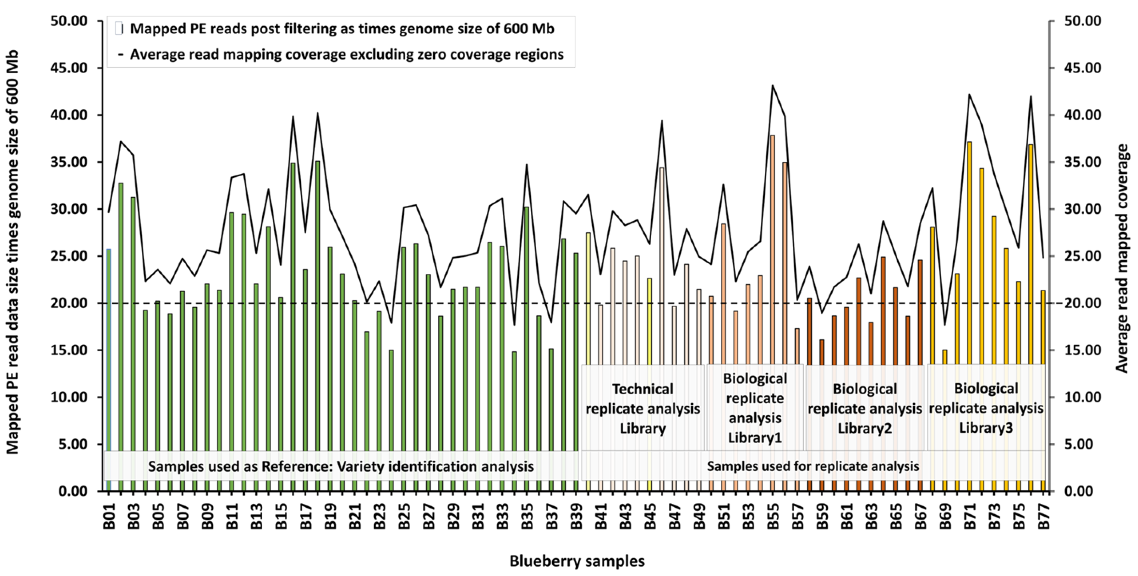
Figure 4.
Identification of an Unknown blueberry sample using uniquely shared Hom-SNPs after filtering Data-noise and Persisting-Data-noise of subclass False-Unique(F1 and F2).
Figure 4.
Identification of an Unknown blueberry sample using uniquely shared Hom-SNPs after filtering Data-noise and Persisting-Data-noise of subclass False-Unique(F1 and F2).
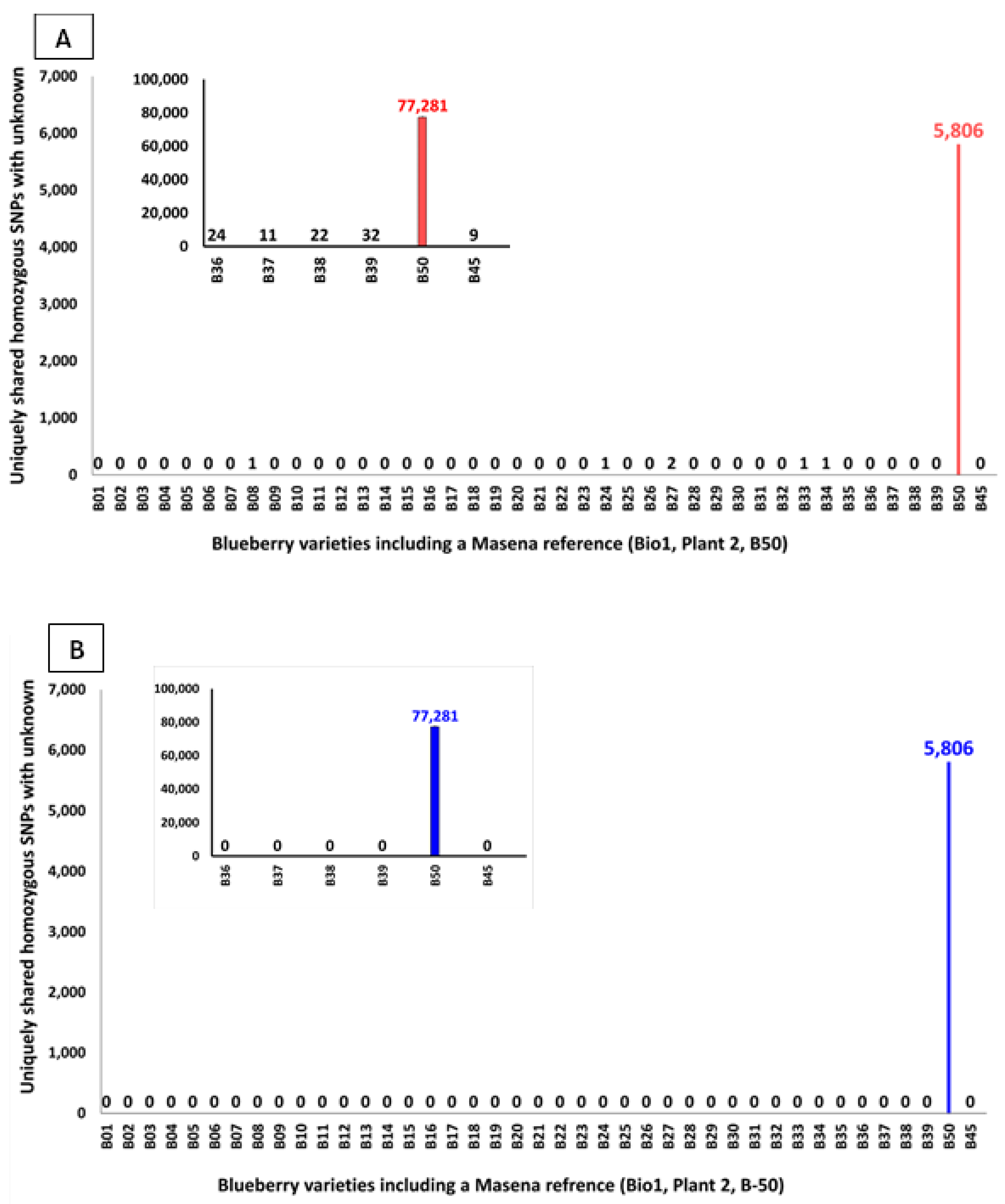

Table 1.
Numbers of false calls of homozygous differences due to chance sequencing of the same allele at a heterozygous position in a diploid.
Table 1.
Numbers of false calls of homozygous differences due to chance sequencing of the same allele at a heterozygous position in a diploid.
| Genome size | Heterozygosity | Sequence coverage | ||
| 10X | 20X | 25X | ||
| Small genome (500 Mbp) | 1% | 4,883 | 5 | 0 |
| 3% | 14,648 | 15 | 0 | |
| Large genome (2 Gbp) | 1% | 19,531 | 19 | 1 |
| 3% | 58,593 | 57 | 2 | |
Table 2.
Percentage probability of heterozygous SNPs erroneously called as homozygous SNP due to read mapping-coverage and read mapping-scenarios.
Table 2.
Percentage probability of heterozygous SNPs erroneously called as homozygous SNP due to read mapping-coverage and read mapping-scenarios.
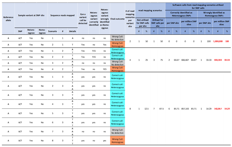 |
Table 3.
Optimal read mapping coverage to reduce the percentage probability of heterozygous SNPs erroneously called as homozygous.
Table 3.
Optimal read mapping coverage to reduce the percentage probability of heterozygous SNPs erroneously called as homozygous.
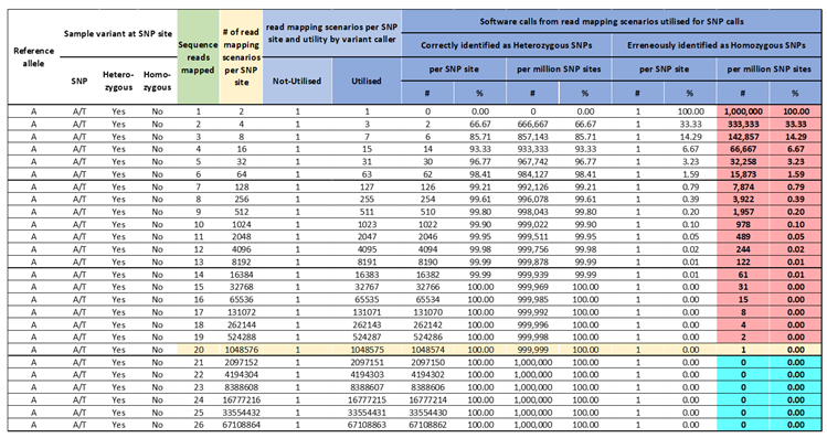 |
Table 4.
Percentage of Common and Not-common Hom-SNPs from PVC analysis of the two blueberry control samples.
Table 4.
Percentage of Common and Not-common Hom-SNPs from PVC analysis of the two blueberry control samples.
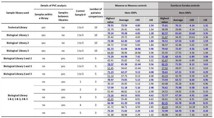 |
Table 5.
Read-mapping scenarios in one sample leading to five subclasses of Not-common SNPs identification in the other sample.
Table 5.
Read-mapping scenarios in one sample leading to five subclasses of Not-common SNPs identification in the other sample.
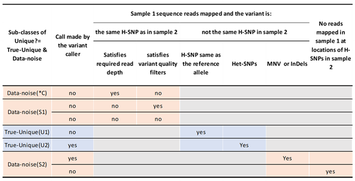 |
Disclaimer/Publisher’s Note: The statements, opinions and data contained in all publications are solely those of the individual author(s) and contributor(s) and not of MDPI and/or the editor(s). MDPI and/or the editor(s) disclaim responsibility for any injury to people or property resulting from any ideas, methods, instructions or products referred to in the content. |
© 2025 by the authors. Licensee MDPI, Basel, Switzerland. This article is an open access article distributed under the terms and conditions of the Creative Commons Attribution (CC BY) license (http://creativecommons.org/licenses/by/4.0/).
Copyright: This open access article is published under a Creative Commons CC BY 4.0 license, which permit the free download, distribution, and reuse, provided that the author and preprint are cited in any reuse.


