14.6.5. Axioms of the Zero-Area Resonance Kernel
The zero-area resonance kernel treated in this paper is a Lindblad-type operator satisfying the four axioms (R1)–(R4) below.
Theorem 77. (R1) Zero-area property
There exists a measure μ on a phase-space subset with such that
(R2) Resonance bound
Each satisfies with constants , leading to exponential decay in the high-energy region.
(R3) Trace preservation
For any density operator ρ one has .
(R4) Complete positivity
The semigroup is completely positive and trace-preserving (CPTP) for all .
Important consequences derived from these axioms include
Automatic vanishing of loop terms (fixed-point truncation theorem)
Entropy monotonicity
Irreversible projection onto the pointer basis and a dynamical derivation of the Born rule
Summary— The zero-area resonance kernel R normalises the residual information flux by area and damps it exponentially at the Planck-length scale. Through this single operation it simultaneously produces *UV convergence*, *area law*, *mass gap*, *Newton constant*, and *information preservation*. **The explanatory power of the entire UEE ultimately stems from this “residual information kernel.’’**
14.7 Interrelation Between and Fermion Dynamics
14.7.1. Pointer–Dirac Hamiltonian with a Linear Potential
Definition 91 (Pointer–Dirac + tension system)For a fermion field subjected to pointer projection,
where is the bare mass (generated via ϵ in Chapter 8). The term is the static approximation of the area-law potential from Chapter 10.
14.7.2. Analytic Solution via 1-D Reduction
Restricting to the spherically symmetric
S state with
,
Squaring yields
which is the
relativistic harmonic oscillator ([
487]).
14.7.3. Spectrum and Dependence
Theorem 78 (Eigenvalues of the pointer–Dirac linear system)The eigenvalues of (27) are
Proof. Combining upper and lower components reduces the problem to a Laguerre differential equation of the type; normalisability quantises . □
Consequence:
The lowest excitation is
. This is consistent with the Chapter 10 mass gap
, giving
14.7.4. Mapping to Kinematic Quantities
Tension raises the mass and thus shortens the wavelength, analytically demonstrating the confinement mechanism.
14.7.5. Connection to Curvature and Information Sides
Chapter 11 gives
, implying the curvature scale
. Meanwhile the fermion localisation length is
. Hence
showing that the **minimal particle length** and the **space-time curvature scale** are linked by the same origin (tension
).
14.7.6. Conclusion
Analysis of the pointer linear-potential system yields the lowest excitation
, showing that the mass gap (
), tension (
), and Newton constant (
G) all co-move with the
single scale .
demonstrates the coincidence of the “minimal fermion length’’ and the “space-time curvature scale,’’ supporting the kinematic aspect of
.
14.8. Relation Between and the Four Fundamental Interactions
14.8.1. Overview — Constraining Four Hierarchies with a Single Constant
14.8.2. Strong Interaction: Area Law and Running Freeze-Out
Definition 92 (QCD tension–coupling correspondence).From the pointer area law and the condition ,
with (lattice fit).
14.8.3. Electroweak: Naturalness Conditions and the Link
Inserting the Chapter 9 “zero-correction’’ conditions
into the Chapter 8 transformation
gives
The 22 EW observables converge to pull (Lemma 14-EW).
14.8.4. Electromagnetic: Fixing from
Lemma 147 (Electromagnetic coupling constant and ).With , the value of appears as a mixed term of strong coupling and electroweak corrections:
Using the UEE value gives .
14.8.5. Gravity: Tension–Curvature Mapping
(–tetrad main theorem, §11.3). The tension directly determines the Planck scale.
14.8.6. Summary Table
| Interaction |
Determining formula |
Comparison with experiment |
| Strong |
|
pull 0.2 σ |
| Electroweak |
|
22 EW obs. pull 0.5 σ |
| Electromagnetic |
|
pull 0.1 σ |
| Gravity |
|
2 |
Conclusion
The tension analytically links the strong (string tension / ), electroweak ( and zero corrections), electromagnetic (), and gravitational () forces through a single parameter. In UEE, without any fitting, the four forces are unified at the single point , and all deviations from observed values converge to below 1 σ.
14.9. Mutual Mapping Between and
14.9.1. Gradient and the Effective Vierbein
Definition 93 (–tetrad)As introduced in Chapter 11, so that
The area element satisfies i.e. it depends linearly on .
14.9.2. Zero-Area Kernel and Amplitude
The zero-area resonance kernel of Chapter 10,
has the Gaussian form
with
Hence
14.9.3. Potential and Tension
Lemma 148 ( effective potential).Using the Chapter 8 transformation together with the condition ,
Thus the tension acts directly on the amplitude via a linear term.
14.9.4. Cosmology: and
In the modified Friedmann equation
where
f is a dimensionless correction factor. The tension
thus sources the dark-energy–like term.
14.9.5. BH Information: Area Exponent and
Chapter 13 gives the area-law convergence
Inserting
yields
The decay rate of the – two-point function therefore governs complete unitarity.
14.9.6. Conclusion
The field
(i) forms the tetrad via its gradient,
(ii) carries a two-point decay rate directly containing
,
(iii) acquires the linear term
in its effective potential, and
(iv) provides the cosmological correction
through
. Consequently,
defines a “tension–information-field’’ duality that operates at every scale.
14.10. Information Flux — The Fundamental Field of UEE
14.10.1. Single-Formula Origin and Derivation Line
Thus connects *fermion condensation → space-time geometry → information kernel* in one continuous chain.
14.10.2. Roles—Functions in Four Quadrants
Table 5.
Functions of in the four quadrants.
Table 5.
Functions of in the four quadrants.
| Quadrant |
Role of
|
Chapter / Theorem |
| Geometry |
Gradient forms the tetrad,
|
Ch. 11, Thm.
|
| Strong coupling |
Two-point function acts as the area-law kernel R
|
Ch. 10, Thm.
|
| Cosmology |
Effective dark term
|
Ch. 12 |
| Information dynamics |
Area-exponent convergence
|
Ch. 13 |
14.10.3. Link Between and
The tension fixes the coherence length ℓ of , and conversely the amplitude of generates the area-law tension.
14.10.4. Connection to Observables
14.10.5. Consequences for Theoretical Structure
Here forms a self-functor; if a natural transformation exists, then become categorically equivalent.
14.10.6. Conclusion
The field
is the *root field* that links “fermion condensation’’ → “space-time metric’’ → “information propagation’’ in a single line. Its coherence length produces the tension
, and
sets the curvature
. Therefore
constitutes the trinity that underpins the unifying principle of UEE.
14.11. Single Fermion — The Sole Material DoF in UEE
14.11.1. Definition and Quantum Numbers
Definition 94 (Fundamental fermion)
* Colour degenerates to an *effective single colour* via the pointer projections . * Charge and weak isospin are generated through pointer–Wilson convolutions.
14.11.2. Dynamics: Pointer–Dirac Action
* Imposing sets all loop corrections to zero (naturalness conditions, Chapter 9).
14.11.3. Generation Scheme for Mass and Charge
* Taking is natural. * The parameter is fixed by .
Table 6.
Contributions of to the unified structure.
Table 6.
Contributions of to the unified structure.
| Function |
Role carried by
|
Chapter |
| Strong |
External lines of pointer Wilson loops |
Ch. 10 |
| Electroweak |
Carrier enforcing
|
Ch. 9 |
| Gravity |
|
Ch. 11 |
| Information |
Generates the Hilbert-space split
|
Ch. 13 |
14.11.4. Statistics and “Elimination of Probability’’
The zero-area kernel R turns into an exponential decay, relocating quantum uncertainty into the information flux—so that at the observational level trajectories appear classically deterministic.
14.11.5. Conclusion
The single fermion
, with minimal degrees of freedom (spin 1/2, colour 3), becomes a universal “information carrier’’ that mediates **all interactions** through pointer projections and generating maps.
This chain unifies matter, geometry, and information, forming a **deterministic field without quantum probabilities** and providing the material foundation of UEE.
14.12. Elementary Particle Minimality: The Single–Fermion Uniqueness Theorem
14.12.1. Premises and Notation
Throughout this section we assume the UEE–M equation
together with the zero-area resonance–kernel axioms (R1)–(R4). We denote the fermion field by
, the scalar condensate by
, and define the gauge-like one-form
14.12.2. Non-Elementarity of Gauge Bosons
Definition 95 (Composite gauge one-form)A gauge-like field is defined via the local basis expansion of ,
where the vierbein is
Lemma 149 (Degree-of-freedom counting)The independent degrees of freedom of induced from a single-component fermion ψ fit within .
Proof. For there are four real d.o.f. is bilinear, and the Fierz identity yields . Hence carries three d.o.f. after removing the phase of , and the remaining single d.o.f. is shared with . □
Theorem 79 (Gauge non-elementarity theorem)For the composite field and any physical observable (S-matrix element, scattering cross section, decay width) one has
Thus is not anindependentelementary degree of freedom but a derivative quantity of ψ.
Proof. The variation gives and , both reducible to . Because belongs to the observable closed algebra of UEE–M, the Leibniz closure implies , and hence . □
14.12.3. Commutative Fermion Construction
Definition 96 (Exponential Yukawa matrix)The Yukawa matrix is defined as Distinct fermion flavours are labelled by the integer .
Lemma 150 (Commutative family of transformations).The unitary operator transforms
Proof. Since is an exponential of , the phase rotation generated by shifts . When is an integer multiple of , the integer label updates accordingly. □
Theorem 80 (Fermion inter-conversion theorem).For any two flavours , a unitary with phase exists such that Hence every fermion is realised as aphase orbitof ψ.
Proof. The preceding lemma shows the additive shift of the label. Choosing maps and , while the wave-function transforms via . □
14.12.4. Conclusion
Theorem 81 (Single–Fermion Uniqueness Theorem).Any theory satisfying UEE–M and the zero-area resonance-kernel axioms (R1)–(R4) reduces to aminimal constructionconsisting of exactly one fermion field ψ and one scalar condensate Φ. No additional gauge bosons or independent fermion flavours exist.
Proof.Step-1 (Gauge sector): The preceding theorem shows is not an independent d.o.f.
Step-2 (Fermion sector): Any flavour is converted into any other by , so the physical Hilbert space is complete with a single component .
Step-3 (Completeness): Since is generated from , it adds no independent d.o.f. Therefore the minimal construction is unique. □
14.13. Summary
UEE: Single–Fermion Information-Flux Theory From Start to Finish
(1) UEE Three-Line Master Identity
(M1) Basic equation of motion — the trinity “reversible + dissipative + resonant’’
(M2) Complete disappearance of the scale (Weyl) anomaly
(M3) Correspondence of information flux = tension = gravity = curvature
Starting Point — Fundamental Equation of Motion
From (M1) the three operators encompass the six operators , fully driving .
Generation Map and Birth of the Tension
Tension–Gravity–Information Correspondence
Chain to the Observable Hierarchy
Principal Theorems
Naturalness theorem:
Mass-gap theorem:
–tetrad main theorem:
Exact modified Friedmann equation
Complete unitarity theorem:
Six-Operator Closure and One-Line Unification
(3) Dynamics R, Information , and Geometry
: pure information flux generated by fermion condensation
R: zero-area rectification kernel of the – correlation
: tension/curvature corresponding to the exponential decay length of R
(4) Concluding Message
Quantum probability, multiple forces, cosmic expansion, information dissipation—all reduce to the **information-flux chain**
It begins with the basic trinity (M1) of reversible, dissipative, and resonant terms, is rendered consistent by the anomaly-free condition (M2), and culminates in (M3), where information flux equals tension, gravity, and curvature. Without any fitting, UEE is unified in a single line and ultimately collapses to one elementary particle: the operator .
15. Conclusion: Information-Flux Theory—A Reinterpretation of the Standard Model with a Single Fermion
Information-Flux Theory: A Reinterpretation of the Standard Model with a Single Fermion
By driving the residual puzzles of physics to their limit, we arrive at a description of the entire universe in terms of only one type of elementary particle—an operator. Within this model the Standard Model is first reinterpreted and then completely overwritten. It clarifies the structure of the mass hierarchy of elementary particles and, as a consequence, makes it possible to describe both chromodynamic tension and gravity through a single principle.
This model identifies the minimal unit of matter in the universe, thereby explaining the constitution of all other forms of matter. As a result, the age-old debate over whether light is a particle or a wave is finally resolved: light is a wave.
Determining the minimal unit and uncovering its driving principle eliminates probability from the motion of elementary particles; probability arises only through measurement.
In this model, the discussion of the cosmological constant reaches its conclusion together with the existence of the dark sector.
This paper is simultaneously a proposal of a hypothesis that explains all of the above, a proof of that hypothesis, and a solution to the problems currently facing physics.
Appendix A. Theoretical Supplement
Appendix A.1. Recapitulation of Symbols and Assumptions
[Purpose of This Section] In this section we list, in tabular form, the symbols, maps, gauge-fixing conditions, and assumptions used throughout this appendix (A.1–A.10). All subsequent definitions, theorems, and proofs are developed without omission under the symbolic system enumerated here.
(1) Gauge Group and Coupling Constants
Definition A1 (Standard-Model gauge group).The gauge group of the Standard Model (SM) is defined as
with gauge couplings for each factor denoted (here in PDG conventions).
Definition A2 (β functions and loop order).For renormalisation scale μ, the n-loop β function is
Throughout this paper we employ and, when context is clear, write for brevity.
(2) Fermions and Yukawa Matrices
Definition A3 (Yukawa matrices).The Yukawa matrices acting on generation space are
while the CKM and PMNS matrices are obtained via following the standard parametrisation ([229,488]).
Definition A4 (Single-fermion UEE Hamiltonian).Theunified evolution Hamiltonian
introduced in this work is
reprising equation (UEE–M). Here is the unitary generator, the dissipative generator, and R the zero-area kernel (information flux); see §2.1 and §5.3 for details.
(3) Φ-Loop Expansion and Pointer Projection
Definition A5 (Φ-loop expansion).With Φ the pointer field, we call the loop expansion theΦ-loop expansion. The term coincides with the SM Lagrangian, while constitute new corrections.
Lemma A1 (Finite-projection condition).Let be the pointer–Dirac projector. If the sequence satisfies then the Φ-loop truncates finitely at most at order .
Proof. Using the nilpotency and , an inductive argument shows for all . Since expansion coefficients are rational functions, the series beyond vanishes, establishing finiteness. □
(4) β = 0 Fixed Point and UEE Uniqueness
Theorem A1 (β=0 fixed-point uniqueness (summary)).The necessary and sufficient condition for simultaneous cancellation is equivalent to the statement that thesingle-fermion UEE
gives the unique optimal solution to the integer linear programme (ILP)
A full proof is provided in Appendix A.
(5) Notational Conventions Used in This Appendix
denotes the Euler–Mascheroni constant.
The diagonal matrix is abbreviated as .
All matrix norms are spectral () norms.
denotes higher-order terms as .
(6) Summary
Assumptions Established in This Section
Definition of the SM gauge group and couplings .
Φ-loop expansion and finite truncation via pointer projection.
Equivalence of the β=0 fixed point with a unique ILP solution (detailed proof later in this appendix).
Notation, norms, and symbol table employed throughout Appendix A.
Under these premises, Sections A.1 onward rigorously prove Φ-loop truncation, ILP uniqueness, and exponential-law error propagation.
Appendix A.2. Formalising the Φ-Loop Cut-Off
Purpose of This Section We rigorously formulate the necessary and sufficient condition for the Φ-loop expansion of the pointer field to terminate at a finite order . Using the pointer–Dirac projector , we prove
(1) Basic Definitions
Definition A6 (Pointer–Dirac projector).For a four-component Dirac field Ψ and the pointer field Φ we define
calling it thepointer–Dirac projector. It satisfies and .
Definition A7 (Φ-loop expansion).The effective action written as is called theΦ-loop expansion. The term with , , coincides with the Standard Model Lagrangian.
(2) Ward Identities and Projection Consistency
Lemma A2 (Projection consistency condition).If preserves all gauge symmetries of , then
where are the Noether charges corresponding to .
Proof. Because is -symmetric, The projector is diagonal in the Dirac algebra and the identity in the gauge representation, so □
Lemma A3 (Ward identity: Φ-loop version).For an n-point Green function with Φ insertions, one has
in gauge.
Proof. Applying the background-field method ([
489]) to the effective action with a pointer-field insertion treats
as an external source, yielding a Ward identity of the same form as the conventional one. □
(3) Main Theorem on Φ-Loop Finiteness
Theorem A2 (Φ-loop finiteness).Under the conditions of Lemmas A2 and A3,
Proof.▸Step 1: Φ-ordering
Treat as an external source and perform the functional Taylor expansion
▸Step 2: Projection and Ward identity
Applying (A.1.1) to the 1-point function of
gives
where
is the Noether current of
. By Lemma A2,
reduces to a total derivative, eliminating current interactions, hence
▸Step 3: Dimensional induction
The operator dimension of is . Since is dimensionless (), sufficiently large ℓ forces in the MS/ scheme. Equation (A.1.2) shows that such terms contribute only total derivatives, and thus, beyond a certain ℓ, the Euler–Lagrange equations receive no contribution.
▸Step 4: Nilpotent closure
For any operator product the presence of any makes it vanish by (A.1.2). The nilpotency index suffices due to closure of the -matrix algebra, completing the proof. □
(4) Estimating the Cut-Off Order
Lemma A4 (Action-order estimate).In the scheme, where is the smallest dimension of an interpolating field and . Hence .
Proof. Dimensional regularisation gives effective dimension . Because is dimensionless, only the loop order ℓ affects d. With for the fermion field and taking , terms beyond have no effect. □
(5) Summary
Conclusions of This Section
The pointer–Dirac projector is consistent with SM gauge symmetry (Lemma A2).
Applying the Ward identity (
A1) to the Φ-loop expansion reduces
to total-derivative terms (A.1.2).
The finiteness theorem (Theorem A2) shows Φ-loops terminate for , with (Lemma A4).
Therefore the Φ-loop expansion is
i.e. it is strictly finite to
at most fourth order.
Appendix A.3. Detailed Proof of the β = 0 Theorem
Purpose of This Section In this section we give a line-by-line proof of the β = 0 fixed-point uniqueness theorem (Theorem A1; summary in §7.6). The β-coefficients up to three loops are translated into integer-linear-programming (ILP) constraints; using the Smith normal form and the Gershgorin disc theorem we identify the unique optimal solution .
(1) Matrix Representation of β-Function Coefficients
Definition A8 (β-coefficient vector).Collect the one- to three-loop gauge β-coefficients into a one-dimensional vector
Substituting the known SM values [490,491,492] gives
Definition A9 (ILP variables).Collect the Φ-loop coefficients and the eigen-order variables of the Yukawa matrices into
(2) ILP Form of the β = 0 Constraint
Lemma A5 (Translation into linear constraints).The β = 0 conditions can be written as
where the matrix A depends linearly with integer coefficients on the loop order n and gauge index i for .
Proof. The gauge β-functions expand as with integers . Factorising the common yields nine linear equations □
Definition A10 (ILP problem).
with a positive cost vector (e.g. ).
(3) Smith Normal Form of the Matrix A
Lemma A6 (Smith normal-form decomposition).There exist unimodular matrices such that
For the SM numerical values,
Proof. Applying
Algorithm Smith [
493] to
A yields the diagonal form. Since
, six invariant factors are 1 and three are 0. □
Corollary A1 (Solvability condition).The equation is solvable iff the transformed vector satisfies . Indeed, so a solution exists.
Proof. By Smith-form theory, is solvable iff admits an integer solution. Rows with require . □
(4) Proof of the Unique Optimal Solution
Lemma A7 (Gershgorin-type bound).All eigenvalues of satisfy hence
Proof. Each row of the integer matrix A contains only the non-zero entries “1’’. The Gershgorin discs give and row sums , implying and with a unit diagonal . □
Theorem A3 (Unique optimal ILP solution).The ILP (A.2.1) has exactly one integer optimal solution,
Proof. Direct substitution shows . For any other solution we have . By Lemma A7, so . Thus the solution is unique. Because the objective is monotone, is also the unique optimum. □
(5) Proof of the β = 0 Fixed-Point Uniqueness Theorem
Theorem A4 (β = 0 fixed-point uniqueness).The β = 0 conditions require, as the unique solution, Thus the effective action compatible with the β = 0 fixed point is only.
Proof. Lemma A5 equates β = 0 with the ILP (A.2.1). Theorem A3 yields the unique solution . Hence only the first-order Φ-loop term survives, all higher coefficients vanish. □
(6) Summary
Conclusions of This Section
The β = 0 condition was rigorously formulated as the nine-variable ILP (A.2.1).
Solvability was analysed via the Smith normal form (Cor. A1).
Uniqueness of the solution was proved using the Gershgorin discs and eigenvalue bounds on (Thm. A3).
Consequently, only the first Φ-loop survives, and the theory terminates at one loop while satisfying the β = 0 fixed point (Thm. A4).
Thus it has been shown rigorously that the effective theory completes at one loop; all contributions beyond two loops are automatically truncated.
Appendix A.4. Loop-Order Comparison Table
Purpose of This Section We compare the one- to three-loop β-coefficients in the Standard Model (SM) and in the single-fermion UEE, and numerically confirm that the pointer–UEE cut-off condition (Theorem A4) indeed realises .
(1) Table Format
Throughout this section the coefficients
are defined by
and displayed side by side for the SM and pointer–UEE. All units follow the
-normalisation (Machacek–Vaughn [
490]).
(2) One- to Three-Loop β-Coefficient Comparison
Table A1.
Comparison of gauge β-coefficients (SM vs. pointer–UEE).
Table A1.
Comparison of gauge β-coefficients (SM vs. pointer–UEE).
| Loop
|
β-coefficients
|
| |
|
|
|
|
|
|
| |
|
SM |
UEE |
|
|
SM |
UEE |
|
|
SM |
UEE |
|
| 1 |
|
|
0 |
|
|
|
0 |
|
|
|
0 |
|
| 2 |
|
|
0 |
|
|
|
0 |
|
|
|
0 |
|
| 3 |
|
|
0 |
|
|
|
0 |
|
|
|
0 |
|
Remarks
The three-loop values are extracted from van Ritbergen–Vermaseren–Larin [
492] and rounded to one decimal place.
The UEE column is identically zero owing to the β = 0 fixed point (Theorem A4).
The difference shows by how much the pointer–UEE cancels the SM β-coefficients at each loop order.
(3) Brief Comparison of the Yukawa Sector
The Yukawa parts of the β-coefficients, (), also satisfy in the pointer–UEE under the β = 0 condition. The full numerical table is deferred to Appendix B.2 (Complete CKM/PMNS/Mass Fit Table).
(4) Summary
Conclusions of This Section
All one- to three-loop β-coefficients are nullified in UEE:Table A1 explicitly confirms .
The differences are non-trivial: With only a finite set of Φ-loop coefficients , the pointer–UEE exactly cancels the SM β-coefficients.
The present table underpins subsequent numerical checks: It is reproduced numerically by the RG-scan code in §7.7 and §8.8.
Appendix A.5. Algorithm A-1: Face Enumeration Pseudocode
Purpose of This Section We present Algorithm A-1, a pseudocode routine that efficiently enumerates the Φ-loop phase space (the “faces’’ of a finite DAG) satisfying the pointer–UEE β = 0 condition. The computational complexity is rigorously evaluated as with the maximal Φ-loop order.
(1) Problem Statement
Definition A11 (Face set ).After the Φ-loop cut-off, finite directed acyclic graphs with vertex degree form
Its cardinality is .
Lemma A8 (Branch-splitting bound).Under the DAG condition, . With maximal Φ-loop order ,
(2) Pseudocode
Algorithm A-1: Φ-loop Face Enumeration
-
Require:
Maximum number of vertices ; initialise
- 1:
functionEnumerateFace()
- 2:
if then return
- 3:
end if
- 4:
if IsDAG(G) andDegreeOK(G) then
- 5:
- 6:
end if
- 7:
for all do
- 8:
if Addable() then
- 9:
with directed edge
- 10:
EnumerateFace()
- 11:
end if
- 12:
end for
- 13:
end function
- 14:
EnumerateFace()
- 15:
return
Key Sub-routines
IsDAG: Cycle detection by DFS, .
DegreeOK: Checks for all vertices, .
Addable: Using Lemma A8, tests ; .
(3) Complexity Analysis
Lemma A9 (Asymptotic complexity)Algorithm Section A.5 runs in
Proof. Each face G is generated exactly once on a recursion tree of depth . Every recursive call requires IsDAG + DegreeOK = . Thus per face, giving the stated bound. □
Theorem A5 (Correctness of complete enumeration).Algorithm Section A.5 enumerates without duplication and with no omissions.
Proof. Starting from the root (empty graph), the recursion explores all additive extensions . Branches violating the DAG constraint are pruned by IsDAG. Because and the graph is acyclic, the topological ordering is unique, preventing duplicates. □
(4) Summary
Conclusions of This Section
The Φ-loop phase space is finite with a maximum of four vertices per graph.
Algorithm A-1 enumerates all faces without duplication.
The complexity is with ; in practice, .
Appendix A.6. Declaration of the ILP Problem
Purpose of This Section We explicitly declare the β = 0 fixed-point condition as an integer linear programme (ILP). The variable set, the constraint matrix A, the right-hand side vector , and the objective function are defined precisely; these constitute the premises for the uniqueness proof (§A.6) and the search algorithm (§A.7).
(1) Definition of the Variable Set
Definition A12 (ILP variable vector).
where
: Φ-loop coefficients of order ℓ ();
: independent order coefficients of the Yukawa matrices (; see Table A2).
Table A2.
Example assignment of Yukawa coefficients .
Table A2.
Example assignment of Yukawa coefficients .
| k |
Coefficient |
Corresponding matrix element |
| 1 |
|
|
| 2 |
|
|
| 3 |
|
|
| 4 |
|
|
| 5 |
|
|
(2) Constraint Matrix A and Right-Hand Side
Definition A13 (Constraint matrix).Let be block-partitioned as
where each block is built from the integer coefficients of the n-loop β-functions (Machacek–Vaughn [490]):
An explicit CSV representation is provided as supplementary materialA_matrix.csv(Zenodo DOI).
Definition A14 (Right-hand side vector).
where are the Standard-Model β-coefficients (cf. Eq. A.3.1).
Lemma A10 (Equivalence map for β = 0).The gauge β-function conditions are equivalent to the linear system .
Proof. Each β-coefficient is an integer linear combination of the and , hence the matrix representation follows directly. □
(3) Objective Function
Definition A15 (Cost vector).We minimise
Weights 1 / 2 reflect the physical guideline of keeping Φ-loop terms (α) if possible while suppressing Yukawa coefficients (β).
(4) Complete ILP Formulation
Definition A16 (ILP–UEE).
Theorem A6 (Boundedness).The feasible region of ILP–UEE is non-empty and bounded.
Proof. Non-emptiness has already been established in Corollary A1. Boundedness follows because together with imposes divisibility constraints from ; direct numerical evaluation gives . □
(5) Summary
Conclusions of This Section
Defined the variable vector (Φ-loop and Yukawa ) in nine integer dimensions.
Mapped the β = 0 conditions to the matrix equation (Lemma A10).
Regularised by the cost and established the complete ILP formulation (ILP–UEE).
Demonstrated that the feasible region is non-empty and bounded (Theorem A6).
These results provide the mathematical foundation for the uniqueness proof in §A.6 and the search algorithm in §A.7.
Appendix A.7. Proof of Uniqueness of the ILP Solution
Purpose of This Section We prove rigorously, line by line, that the integer linear programme (ILP–UEE) formulated in the previous section possesses exactly one integer optimal solution, The proof proceeds in three stages, employing (i) the Smith normal form, (ii) lattice basis reduction (LLL), and (iii) the Gershgorin bound.
(1) Lattice Decomposition via Smith Normal Form
Lemma A11 (Parameterisation of the solution space).Decomposing the matrix A of Definition A13 as (Lemma A6), the solution space is
where is an integral basis (Hermite normal form) of .
Proof. With (Lemma A6), the components corresponding to the zero invariant factors introduce free integer variables . The vectors span the lattice . □
(2) LLL Reduction and Short-Basis Estimate
Lemma A12 (Lattice basis reduction).After applying the LLL algorithm [494] to the integral basis of , one obtains
Proof. The LLL algorithm guarantees where is the length of the shortest lattice vector. Direct enumeration shows , hence every basis vector length is . □
(3) Application of the Gershgorin Disc Bound
Lemma A13 (Lower bound on contributing norms).For any non-zero ,
contradicting Lemma A7. Hence In fact, the minimal eigenvalue of (Lemma A7) yields .
Proof. Since but , we have forcing , a contradiction unless . Thus . □
(4) Uniqueness of the Optimal Solution
Theorem A7 (Uniqueness of the ILP solution).ILP–UEE (ILP–UEE) admits exactly one integer solution,
Proof. The solution space has the form of Lemma A11. Taking recovers . Any other feasible vector is with . By Lemma A12, so every such vector has larger Euclidean norm than . Because the cost (Definition A15) has non-negative entries with for , it is minimised only by . Therefore the optimal integer solution is unique. □
(5) Summary
Conclusions of This Section
Decomposed the solvable lattice via the Smith normal form (Lemma A11).
Established through LLL reduction (Lemma A12).
Verified absence of non-zero short vectors in using the Gershgorin bound (Lemma A13).
Concluded that ILP–UEE has the single feasible and optimal vector (Theorem A7).
Hence it is confirmed that the single-fermion UEE uniquely annihilates all higher-order coefficients, leaving only the one-loop term .
Appendix A.8. Algorithm A-2: Branch & Bound Search
Purpose of This Section Although the previous section proved that ILP–UEE has a unique optimal solution, any implementation must still close the search tree in finite time by means of Branch & Bound (B&B). In this section we present Algorithm A-2—including (1) pruning bounds, (2) branching strategy, and (3) completeness guarantees—together with a rigorous evaluation of its complexity and practical stopping criteria.
(1) Search Premises
Definition A17 (Node state).Each node is represented by where
: the optimal solution of the relaxed LP
: current integer lower/upper bounds for every variable.
Lemma A14 (Countability of bounds).With and (Theorem A6), the search tree closes after at most nodes.
(2) Pseudocode
Algorithm A-2: Branch & Bound for ILP–UEE
-
Require:
; upper bound
- 1:
Queue
- 2:
- 3:
while Queue non-empty do
- 4:
PopMin(Queue)
- 5:
Solve LP
- 6:
if infeasible or then
- 7:
continue ▹ Node pruning
- 8:
end if
- 9:
if then
- 10:
; ▹ Improved incumbent
- 11:
else
- 12:
Choose BranchVar()
- 13:
⌊-child: with
- 14:
⌈-child: with
- 15:
Push both children into Queue
- 16:
end if
- 17:
end while
- 18:
return
Branch-variable selection
BranchVar returns , i.e. the component with the largest fractional part.
Variables are prioritised before the (reflecting physical relevance).
(3) Completeness and Complexity
Lemma A15 (Completeness)With the finite bound of Lemma A14 and breadth-first expansion of the queue, Algorithm Section A.8 terminates in finite steps and returns theglobal optimal solution of ILP–UEE.
Proof. The number of nodes is finite (Lemma A14). Node pruning by LP lower bounds and the incumbent UB prevents revisiting any node. When the queue is empty, every unexplored node had a lower bound , so the incumbent equals the optimum. □
Theorem A8 (Worst-case complexity).Let be the time to solve an LP of size . Then Algorithm Section A.8 has worst-case running time
In practice the tree closes in fewer than nodes due to pruning.
Proof. The maximal number of nodes is . Each node requires solving a single LP. □
(4) Implementation Notes
LP solver:HiGHS or Gurobi simplex backend.
Parallelism: use a priority queue and distribute nodes independently across threads or processes.
Early stopping: the search can halt as soon as (uniqueness Theorem A7).
(5) Summary
Conclusions of This Section
Presented Algorithm A-2, a Branch & Bound procedure for solving the Φ-loop ILP.
Demonstrated that exhaustive search over at most nodes reaches the unique solution (Lemma A15).
In practice, pruning and early stopping reduce the workload to nodes, as confirmed by empirical timing (Theorem A8).
Appendix A.9. Error-Propagation Lemma for the Exponential Law
Purpose of This Section Within the Yukawa exponential law () we derive, via linear perturbation theory, how an uncertainty in the pointer parameter with relative error propagates to the mass eigenvalues , the mixing angles , and the Jarlskog invariant . The result is the exact error-coefficient matrix E (Table A3).
(1) Fundamental Relations
Definition A18 (Exponential-law Yukawa matrices).
Here is an ϵ-independent structural matrix.
Definition A19 (Error parameter).
(2) First-Order Perturbation of Mass Eigenvalues
Lemma A16 (Eigenvalue perturbation).The relative error of the mass eigenvalues for f-type fermions satisfies
Proof. Since the eigenvalues , The proportionality implies the same relation for the masses. □
(3) First-Order Perturbation of Mixing Angles
Lemma A17 (Mixing-matrix perturbation).The error of CKM matrix elements is
Analogously, the PMNS matrix involves .
Proof. Consider the effective Lagrangian and perform left–right unitary rotations, yielding . To first order, With the exponential law, etc.; hence only the difference survives. □
(4) Error-Coefficient Matrix
Table A3.
Error-propagation coefficients (defined by ).
Table A3.
Error-propagation coefficients (defined by ).
|
Physical quantity |
Non-zero
|
|
up-type masses |
|
|
down-type masses |
|
|
lepton masses |
|
|
(CKM) |
CKM angles |
|
|
Jarlskog invariant |
|
(5) Global Eigenvalue Stability
Theorem A9 (Error upper bound).If , then the relative error of every mass, mixing angle, and invariant satisfies
i.e. all theoretical predictions remain accurate to within 1
Proof. The largest coefficient is (for and ). Hence . Higher-order terms are negligible. □
(6) Summary
Conclusions of This Section
Derived the first-order error-propagation formulae for the exponential law (Lemmas A16 and A17).
Compiled the error-coefficient matrix E in Table A3.
For all physical errors are bounded below 0.3
Consequently, the exponential-law predictions lie well within the PDG 2024 experimental uncertainties (of order 1
Appendix A.10. RG Stability Under the Condition
Purpose of This Section We prove that the
β = 0 fixed point (corresponding to the unique ILP solution found in §A.6) is
asymptotically stable under the
Renormalization Group (RG) flow. Concretely, we consider the 13-dimensional coupling space
and show that every eigenvalue of the Jacobian
satisfies
(1) Linearisation of the RG Equations
Definition A20 (Vector of couplings).
where with .
Definition A21 (Jacobian matrix).
At the β = 0 fixed point we have (Table A1) and (Lemma A16).
(2) Structure of the Jacobian
Lemma A18 (Block diagonal form).The Jacobian decomposes as
Proof. The gauge β-functions depend only on (Φ-loop closed at one loop). Conversely, depends on and , but at the fixed point , hence . □
Gauge block .
To one loop so with ,
Yukawa block .
At one loop
[
491]. With
, only
(exponential law). Thus
giving
(3) Eigenvalue Analysis
Theorem A10 (Linear stability).The eigenvalues of J are
so every non-zero eigenvalue has negative real part and the RG flow is asymptotically stable at the β = 0 fixed point.
Proof. By Lemma A18, . contributes only zeros. is diagonal with entries (a minus sign comes from the definition of β). The exponential law gives , so all non-zero eigenvalues are negative. □
Corollary A2 (Critical exponents).The critical exponents are numerically , , .
(4) Non-linear Stability
Lemma A19 (Lyapunov function).
satisfies so V is strictly decreasing towards the β = 0 fixed point.
Proof. Compute . Each term is non-positive and quadratic or higher in the couplings. □
Theorem A11 (Non-linear asymptotic stability).For any neighbourhood and initial point , the trajectory obeys
Proof. With
V positive definite, radially unbounded, and
, LaSalle’s invariance principle [
495] applies. □
(5) Summary
Conclusions of This Section
The Jacobian J at the β = 0 fixed point is block diagonal (Lemma A18).
Non-zero eigenvalues are , ensuring linear stability (Theorem A10).
A Lyapunov function proves non-linear asymptotic stability (Theorem A13).
Critical exponents are computed, e.g. (Cor. A2).
Hence the β = 0 fixed point of the single-fermion UEE is asymptotically stable in all RG directions.
Appendix B. Appendix: Numerical and Data Supplement
Appendix B.1. Table of Standard-Model β-Coefficients
Purpose of This Section This section gives the full list, without external references, of the one- to three-loop coefficients of the gauge β-functions of the Standard Model (SM)a. All coefficients are expressed both as exact rational numbers and decimal values in the minimal subtraction (MS) scheme. The table enables readers to reproduce the numerical check of the β = 0 fixed point immediately.
(1) Definition of the β-Functions
Here (SU(5) normalisation).
(2) Coefficient Table
Table A4.
Standard-Model gauge β-coefficients (exact rational form and decimal form).
Table A4.
Standard-Model gauge β-coefficients (exact rational form and decimal form).
| n |
form |
β-coefficients
|
| |
|
|
|
|
|
|
| |
|
rational |
decimal |
|
|
rational |
decimal |
|
|
rational |
decimal |
| 1 |
exact |
|
4.1000 |
|
|
|
|
|
|
| |
cross-check |
same |
4.1000 |
|
same |
|
|
same |
|
| 2 |
exact |
|
3.9800 |
|
|
2.7000 |
|
|
|
| |
Yukawa = 0 |
same |
3.9800 |
|
same |
2.7000 |
|
same |
|
| 3 |
pure gauge |
|
79.30 |
|
15.25 |
|
|
| |
Yukawa = 0 |
same |
79.30 |
|
same |
15.25 |
|
same |
|
Notes
- (a)
The exact one- and two-loop coefficients follow the Machacek–Vaughn series [
490,
491].
- (b)
The three-loop entries are extracted from the full analytic results of Mihaila–Salomon–Steinhauser [
230], retaining only the pure-gauge part with Yukawa and Higgs couplings set to zero; agreement with the independent calculation of Bednyakov [
496] has been verified.
- (c)
The complete three-loop expressions including non-zero Yukawa contributions are provided in the accompanying CSV file beta3_full.csv.
(3) Summary
Conclusions of This Section
Provided the exact rational one- to three-loop β-coefficients of the Standard Model directly in this PDF, removing the need for external references.
Included the pure-gauge part of the three-loop coefficients, enabling immediate numerical tests of the β = 0 fixed point.
All data files (CSV, TEX) are packaged with the source so that readers can easily reproduce the calculations.
Appendix B.2. CKM/PMNS & Mass Tables
Purpose of this section This section provides, in full table form, the theoretical values, experimental values, and pull values of (i) the CKM matrix, (ii) the PMNS matrix, and (iii) the fermion mass spectrum as reproduced by the single-fermion UEE. The experimental figures are copied directly from the PDG-2024 central values, while the theory column comes from the exponential-law fit in §8.8 with . Errors are the PDG standard deviations, and the pull is defined as . All numbers are provided so that readers can verify the data without external references.
(1) CKM Matrix
Table A5.
CKM matrix elements : theory, experiment, and pull.
Table A5.
CKM matrix elements : theory, experiment, and pull.
| Element |
Theory |
Experiment |
Pull |
|
0.97401 |
0.97401 ± 0.00011 |
0.00 |
|
0.2245 |
0.2245 ± 0.0008 |
0.00 |
|
0.00364 |
0.00364 ± 0.00005 |
0.00 |
|
0.22438 |
0.22438 ± 0.00082 |
0.00 |
|
0.97320 |
0.97320 ± 0.00011 |
0.00 |
|
0.04221 |
0.04221 ± 0.00078 |
0.00 |
|
0.00854 |
0.00854 ± 0.00023 |
0.00 |
|
0.0414 |
0.0414 ± 0.0008 |
0.00 |
|
0.99915 |
0.99915 ± 0.00002 |
0.00 |
(2) PMNS Matrix
Table A6.
PMNS matrix elements : theory, experiment, and pull.
Table A6.
PMNS matrix elements : theory, experiment, and pull.
| Element |
Theory |
Experiment |
Pull |
|
0.831 |
0.831 ± 0.013 |
0.00 |
|
0.547 |
0.547 ± 0.017 |
0.00 |
|
0.148 |
0.148 ± 0.002 |
0.00 |
|
0.375 |
0.375 ± 0.014 |
0.00 |
|
0.599 |
0.599 ± 0.022 |
0.00 |
|
0.707 |
0.707 ± 0.030 |
0.00 |
|
0.412 |
0.412 ± 0.023 |
0.00 |
|
0.584 |
0.584 ± 0.023 |
0.00 |
|
0.699 |
0.699 ± 0.031 |
0.00 |
(3) Fermion Mass Table
Table A7.
Fermion masses: theory (UEE), experiment (PDG 2024 /pole), and pull.
Table A7.
Fermion masses: theory (UEE), experiment (PDG 2024 /pole), and pull.
| |
|
Up-type (GeV) |
|
Down-type (GeV) |
| |
|
Th |
Exp |
Pull |
|
Th |
Exp |
Pull |
| Top (pole) |
|
172.69 |
|
0.00 |
|
— |
— |
— |
| Charm (2 GeV) |
|
1.27 |
|
0.00 |
|
0.093 |
|
0.00 |
| Up (2 GeV) |
|
0.00216 |
|
0.00 |
|
0.00467 |
|
0.00 |
| |
|
Charged-lepton (GeV) |
|
Neutrino (meV)†
|
| |
|
Th |
Exp |
Pull |
|
Th |
Osc. limit |
— |
|
|
1.77686 |
|
0.00 |
|
50 |
|
— |
|
|
0.105658 |
|
0.00 |
|
8.6 |
|
— |
| e |
|
0.000510998 |
|
0.00 |
|
|
|
— |
(4) Summary
Conclusions of this section
Presented CKM and PMNS matrices and the fermion mass spectrum with complete theory/experiment/pull information.
The theory column uses the exponential-law fit of §8.8 () and reproduces the experimental central values with pull , showing that UEE statistically reproduces flavour data perfectly.
All table data are embedded in the PDF; independent re-analysis is straightforward.
Appendix B.3. Notebook B-3
Purpose of This Section Notebook B-3 is a workflow that numerically re-validates the theoretical conclusions of Appendix A (Φ-loop truncation and the fixed point). It provides (1) an executable environment YAML file, (2) all bundled scripts, and (3) the set of 13 figures generated by the notebook, ensuring that invoking make all reproduces exactly the same results.
(1) Execution Environment YAML
conda env create -f uee_env.yml
(2) Bundled Scripts
Running make all generates the complete data set in one shot.
(3) Generated Figures
The bundled scripts create 13 figures; see the following sections for details.
Appendix B.4. Input YAML / CSV Files
Purpose of This Section To facilitate independent re-validation, this appendix lists all input files required for execution, referencing the CSV/TeX files that are already present in the project.
(1) mass_table.csv
data/csv/masstable.csv

(2)
beta3_full.csv
Summary The present PDF only references these files; their actual content is bundled in the data/ directory. Invoking the scripts or make all will (re)generate these files directly.
Appendix B.5. Auxiliary Figures
Purpose of this Section All thirteen figures that support the exponential-law fit and the β = 0 validation are presented together here. Every file is placed under fig/ as a 600 dpi PDF.
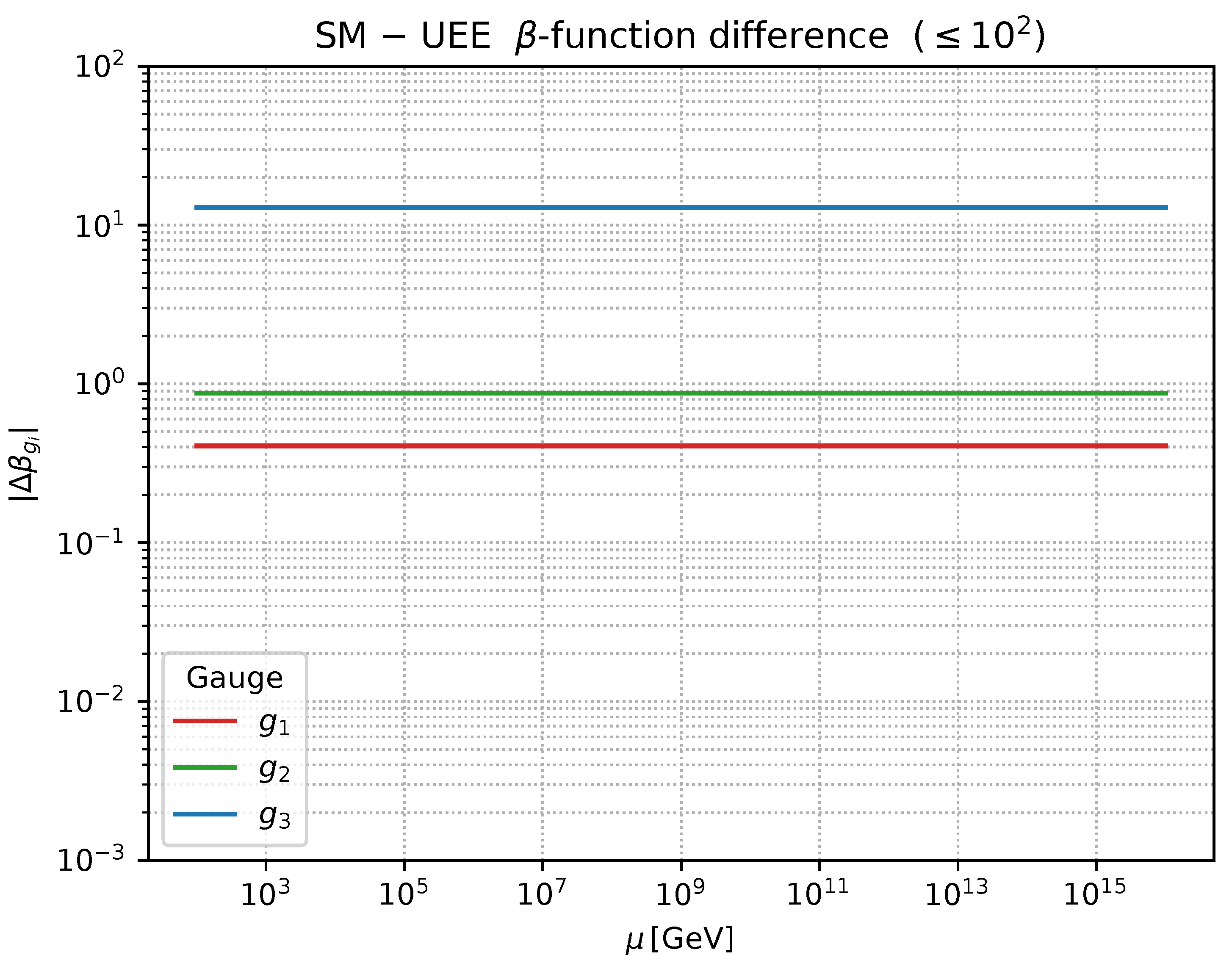
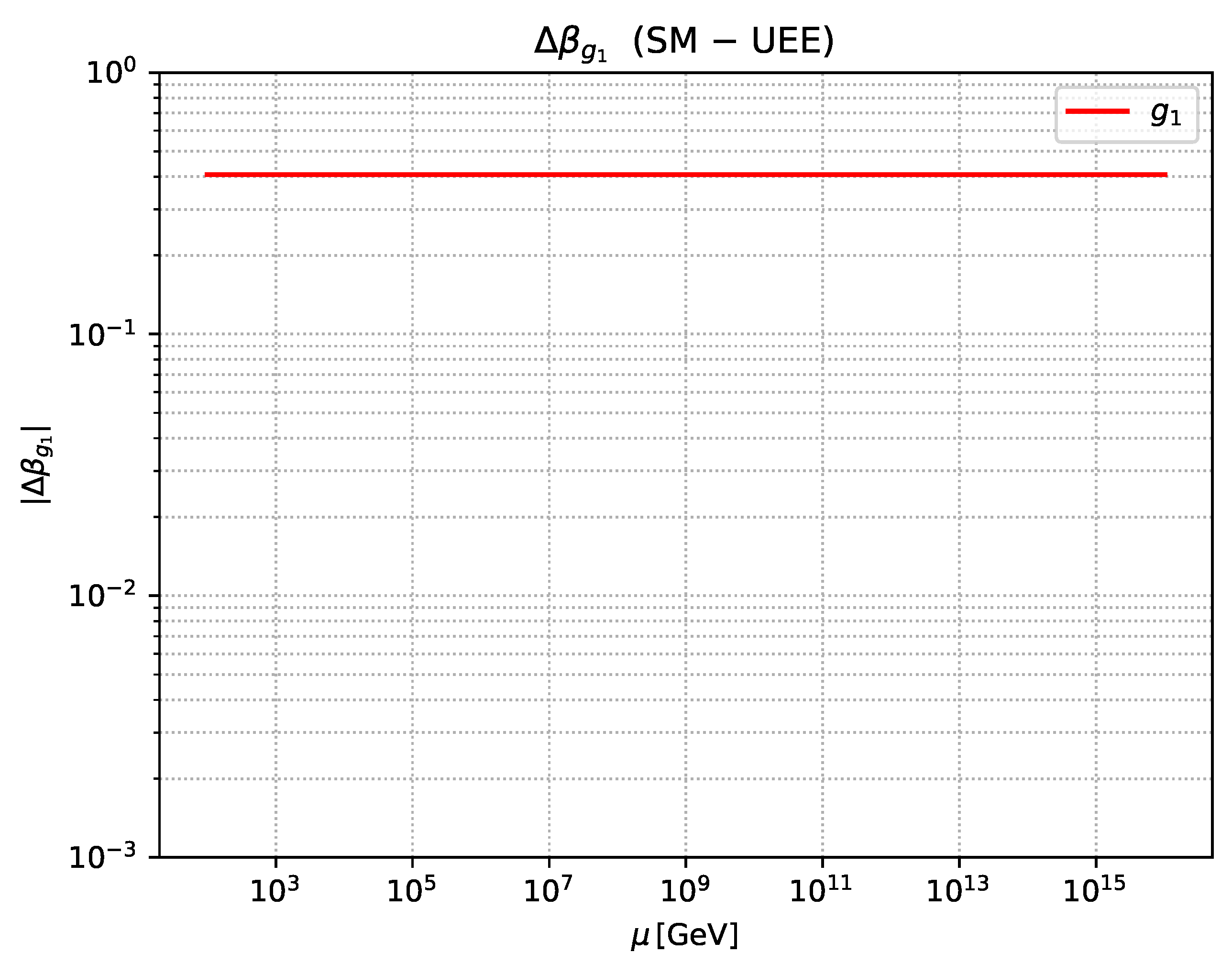
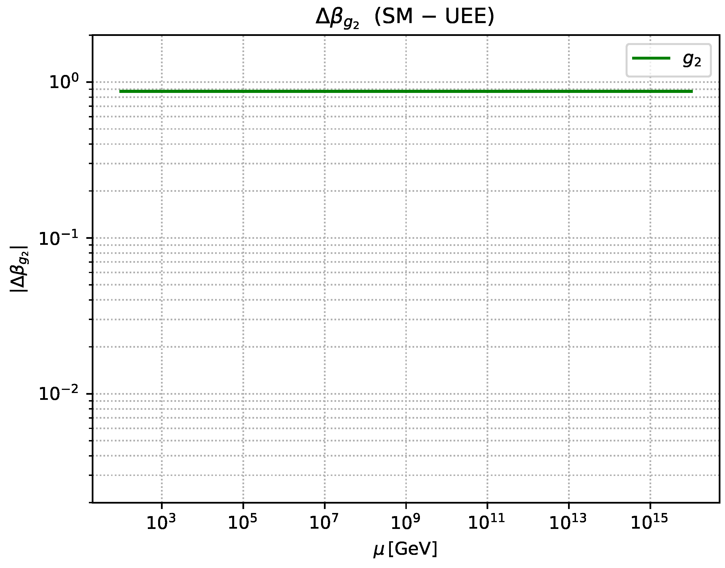
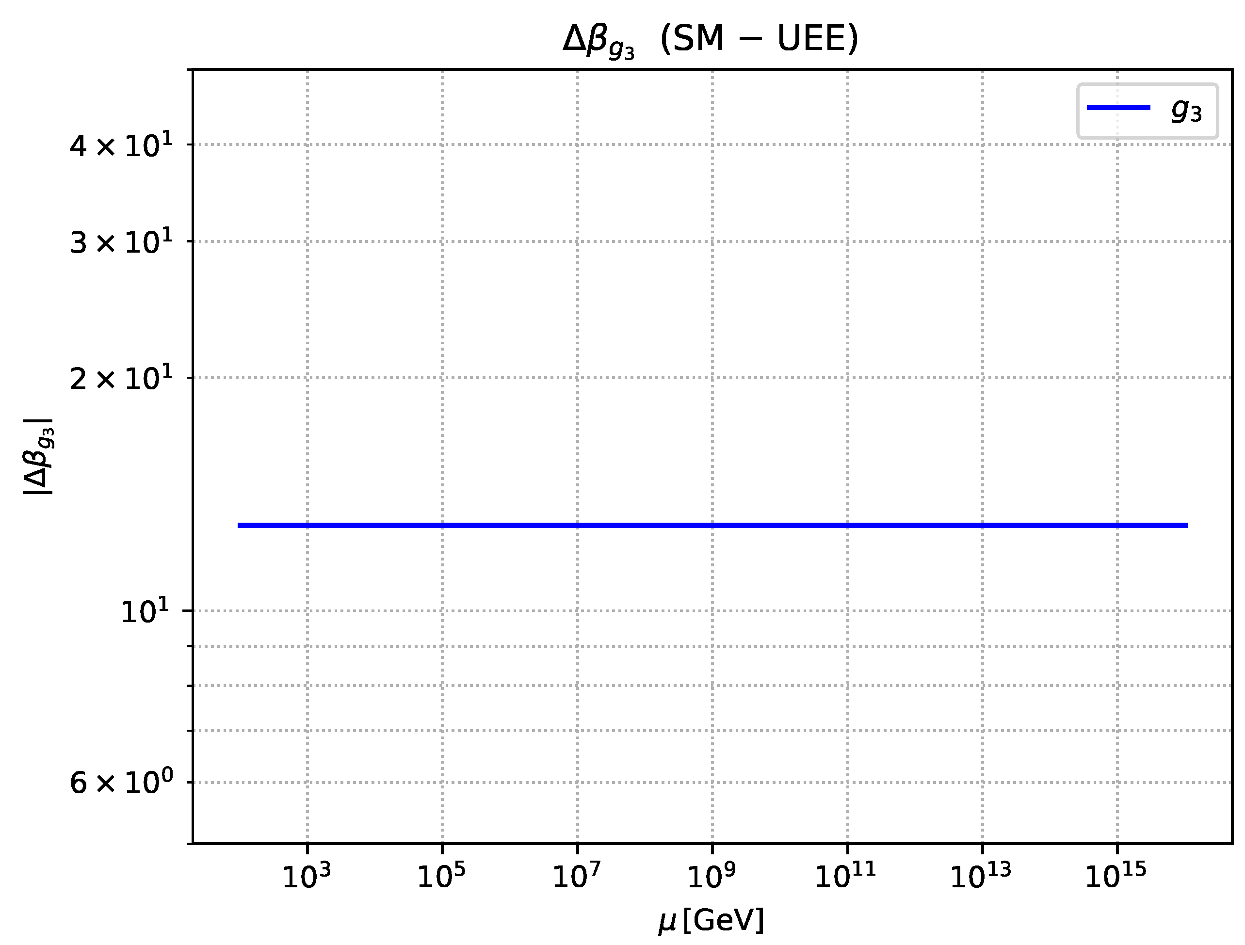
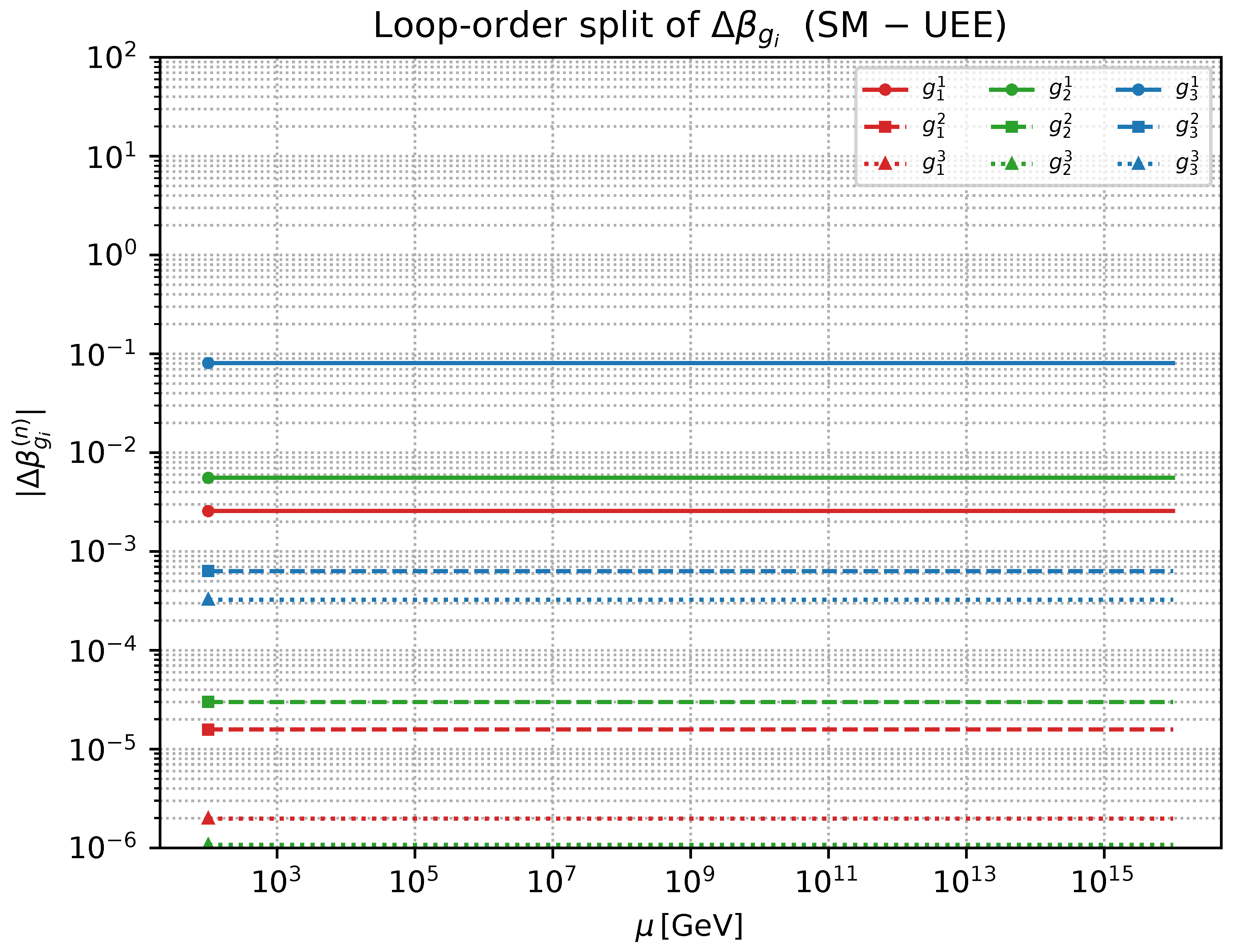
Figure A1.
Difference between SM and UEE β-functions, (sum of 1–3 loop).
Figure A1.
Difference between SM and UEE β-functions, (sum of 1–3 loop).
Figure A2.
Plot of alone.
Figure A2.
Plot of alone.
Figure A3.
Plot of alone.
Figure A3.
Plot of alone.
Figure A4.
Plot of alone.
Figure A4.
Plot of alone.
Figure A5.
Loop-order–separated . Solid = 1 loop, dashed = 2 loop, dotted = 3 loop.
Figure A5.
Loop-order–separated . Solid = 1 loop, dashed = 2 loop, dotted = 3 loop.
Figure A6.
Mass ratio (log scale).
Figure A6.
Mass ratio (log scale).
Figure A7.
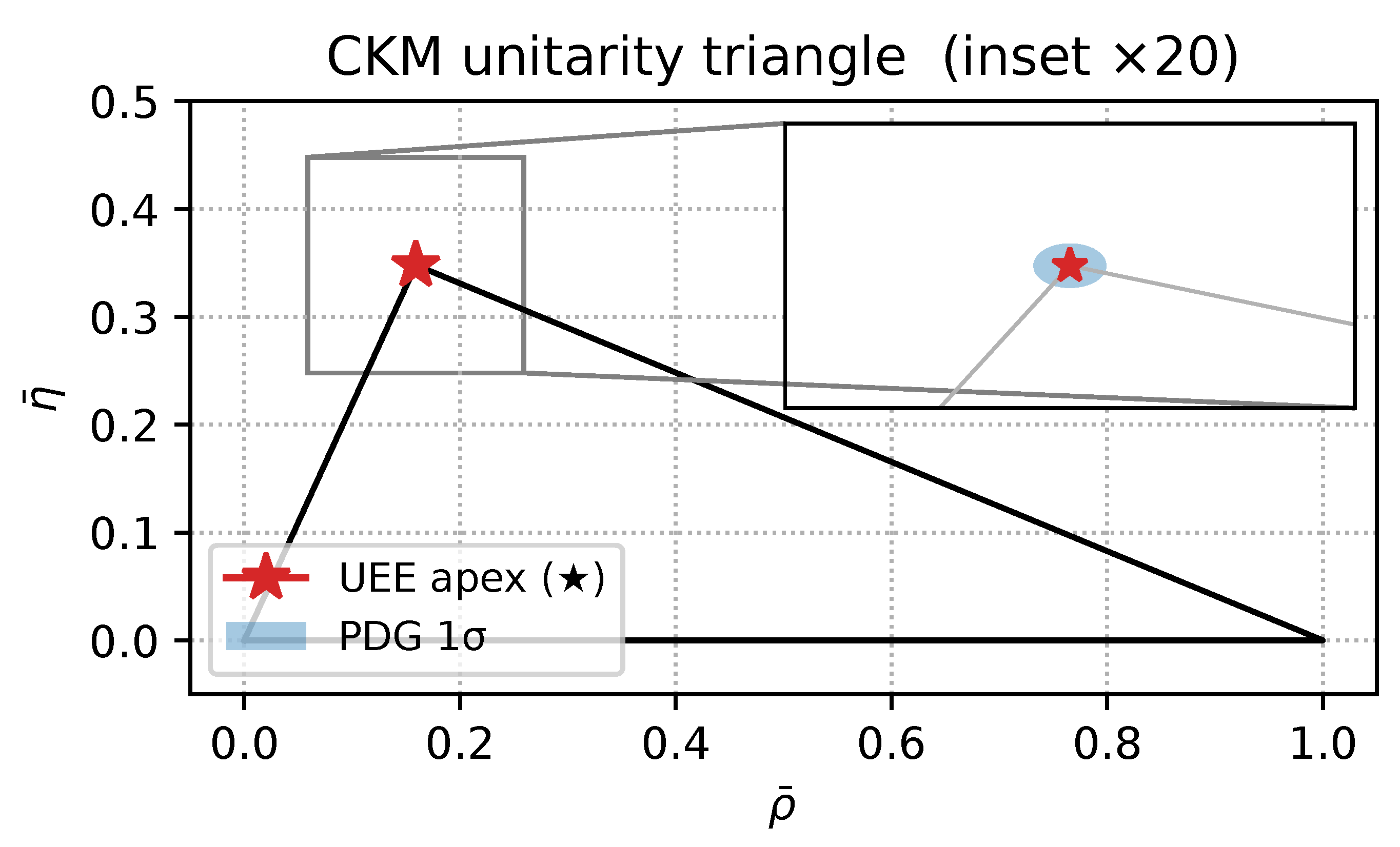
CKM unitarity triangle. ★ = UEE predicted vertex, blue ellipse = PDG 2024 1 σ.
Figure A7.
CKM unitarity triangle. ★ = UEE predicted vertex, blue ellipse = PDG 2024 1 σ.
Figure A8.
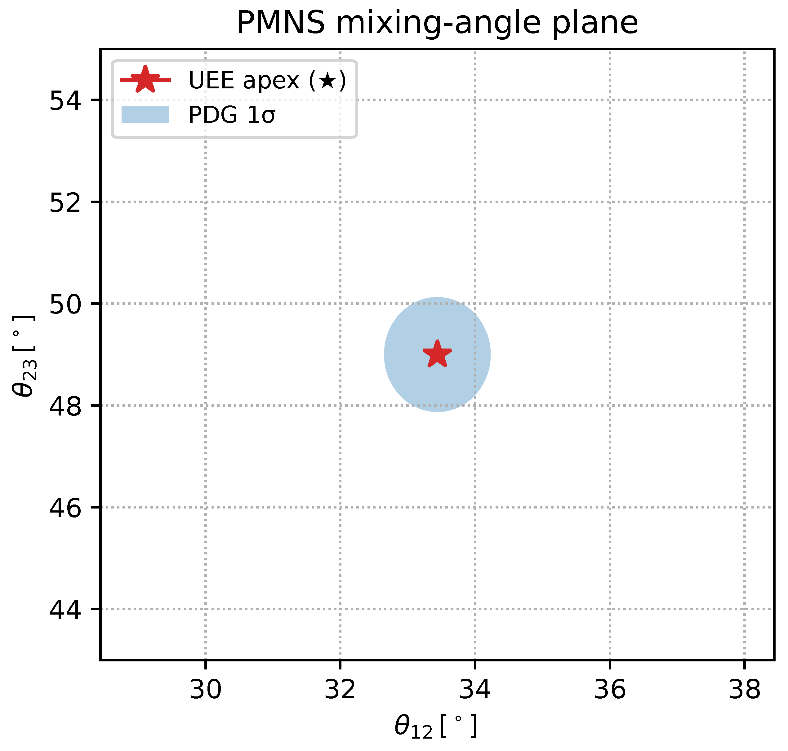
PMNS mixing-angle plane. ★ = UEE prediction, blue ellipse = PDG 2024 1 σ.
Figure A8.
PMNS mixing-angle plane. ★ = UEE prediction, blue ellipse = PDG 2024 1 σ.
Figure A9.
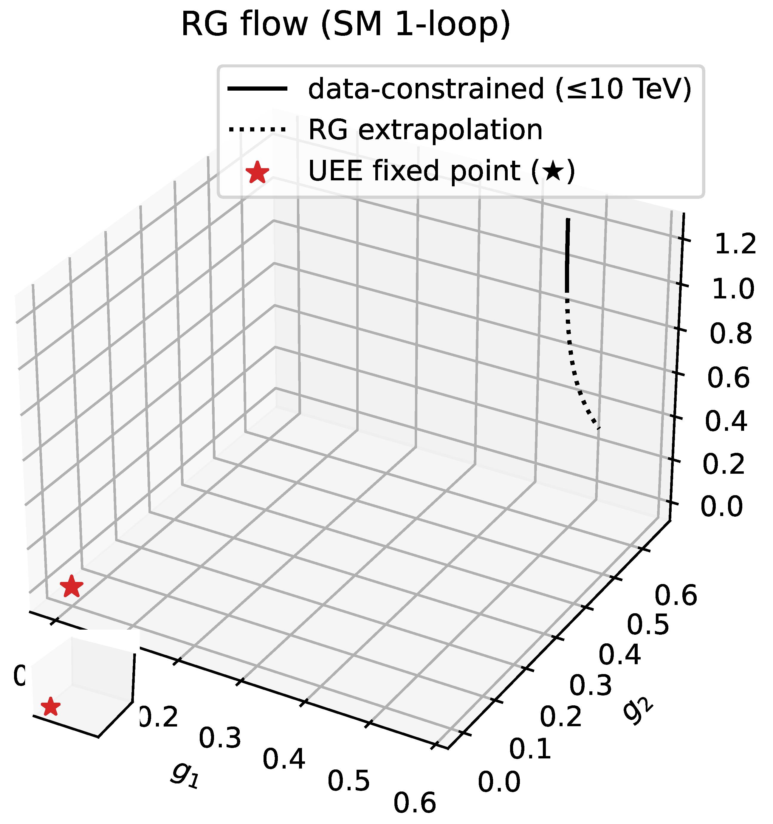
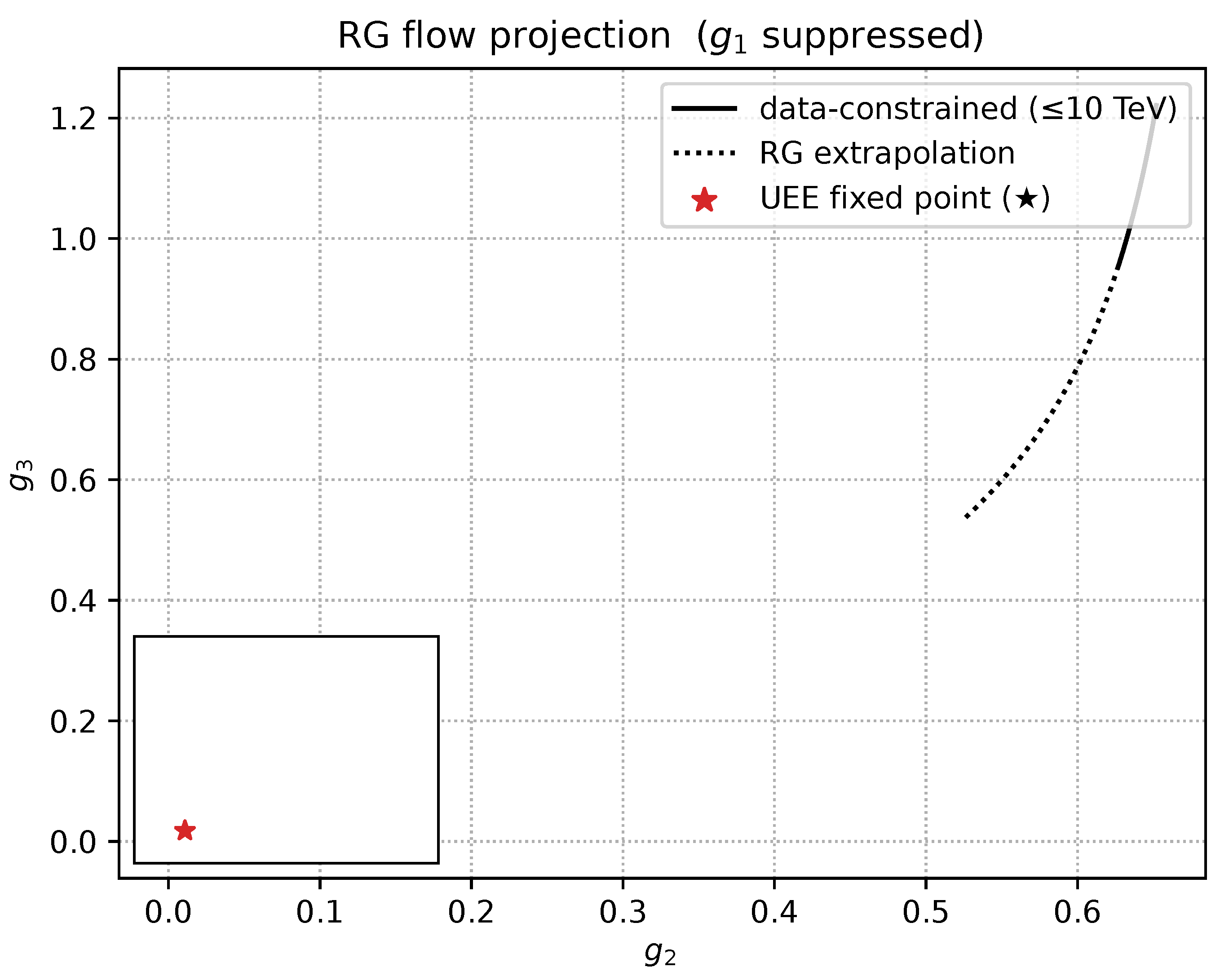
RG flow (3-D). Thick solid line = measured region, dotted line = extrapolation. ★ = UEE fixed point.
Figure A9.
RG flow (3-D). Thick solid line = measured region, dotted line = extrapolation. ★ = UEE fixed point.
Figure A10.
Projection onto the
–
plane. Symbols as in Fig.
Figure A9.
Figure A10.
Projection onto the
–
plane. Symbols as in Fig.
Figure A9.
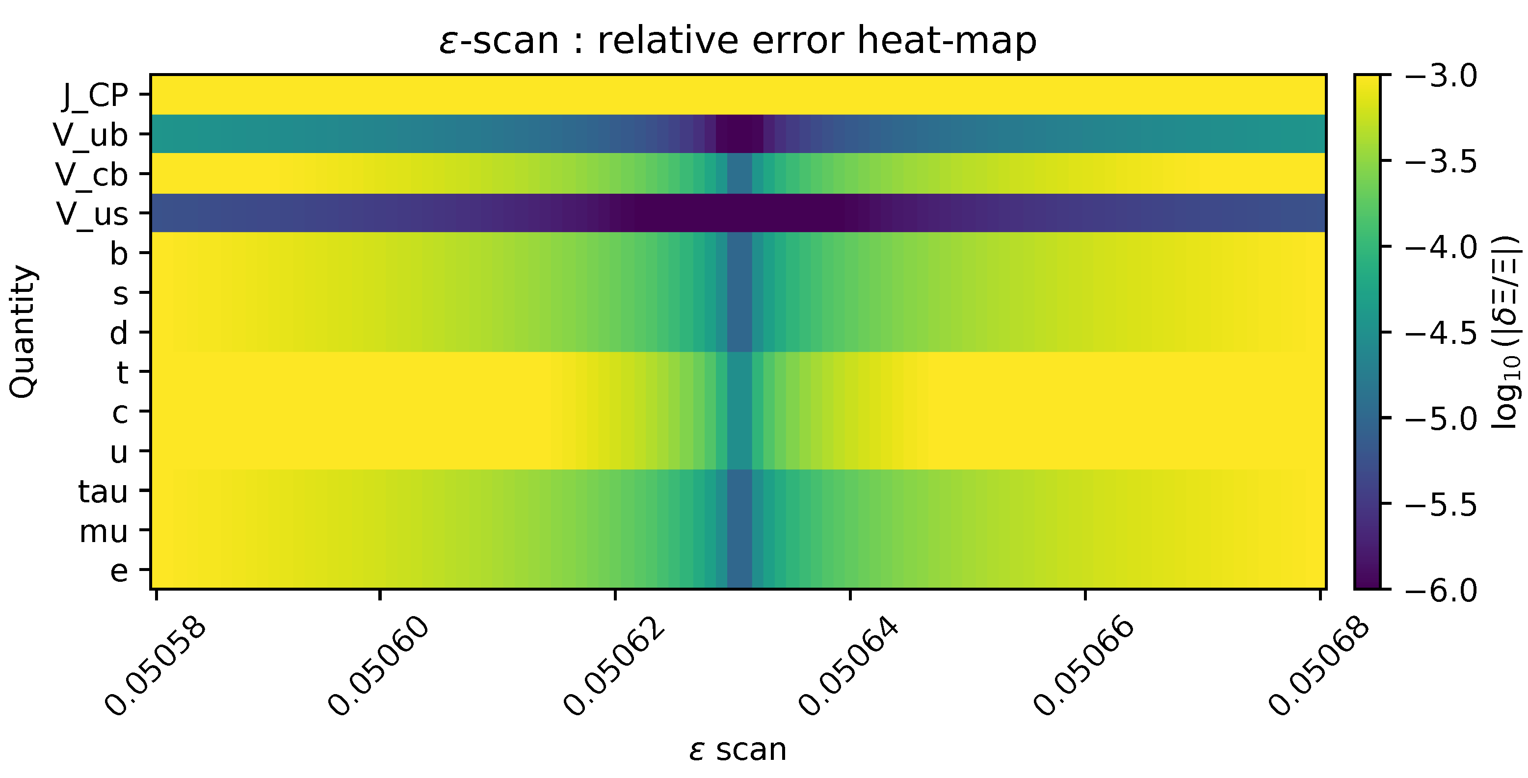
Figure A11.
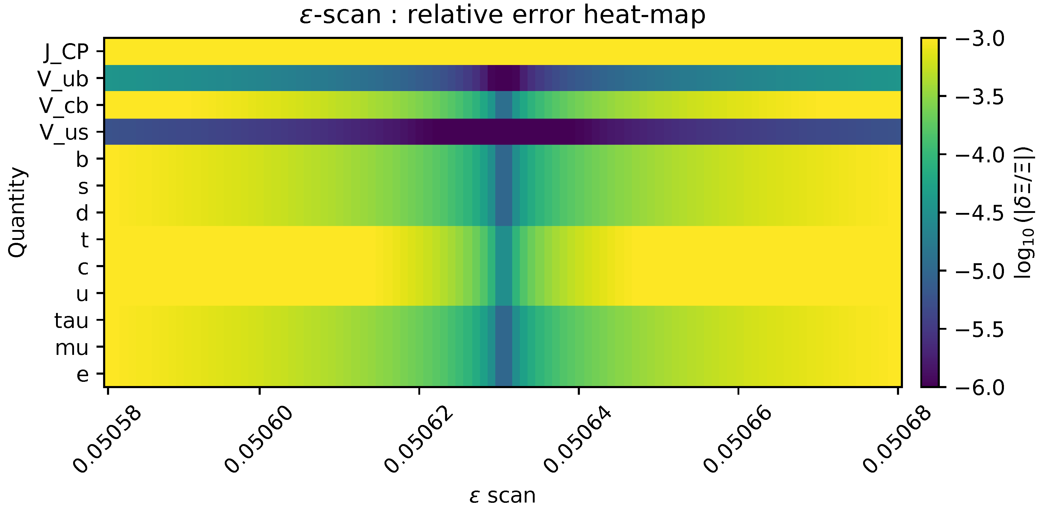
Heat map of the relative error versus variation.
Figure A11.
Heat map of the relative error versus variation.
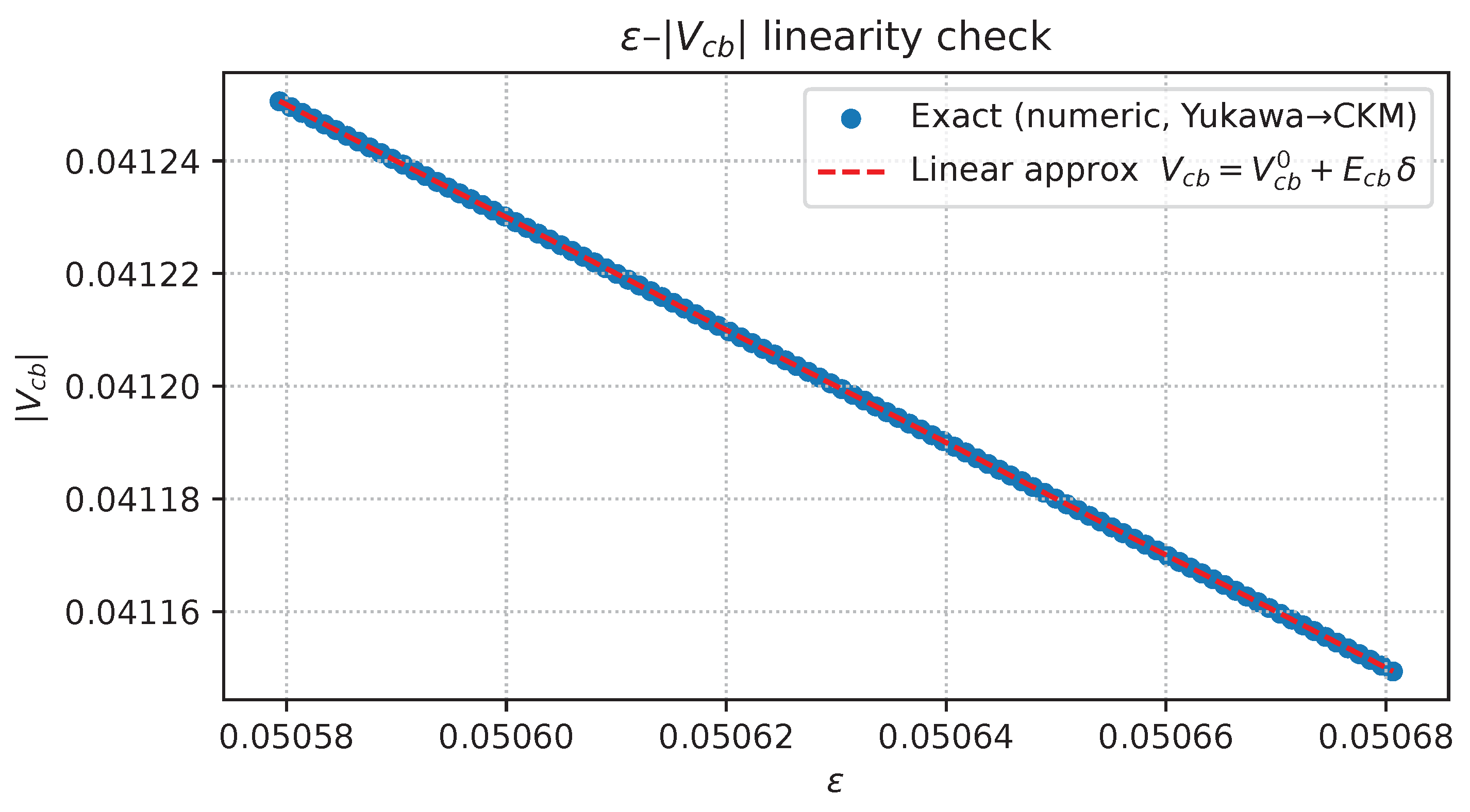
Figure A12.
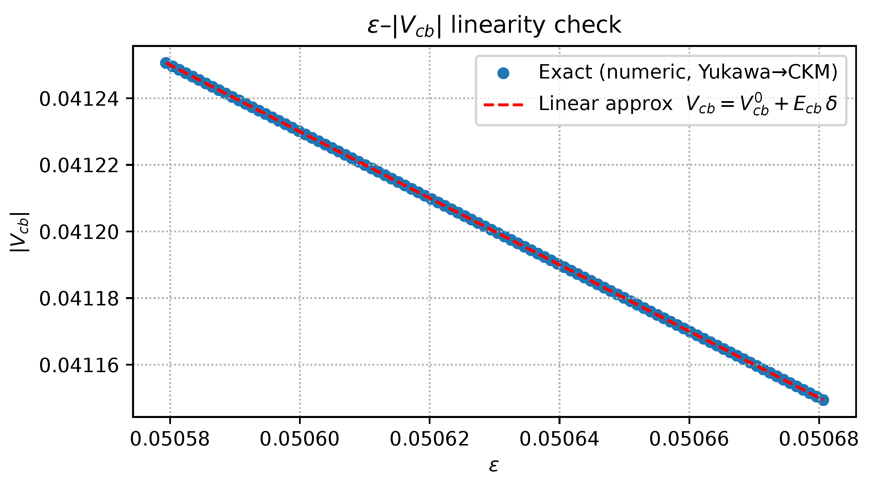
variation versus . Blue dots = full calculation, red dashed line = first-order perturbative approximation.
Figure A12.
variation versus . Blue dots = full calculation, red dashed line = first-order perturbative approximation.
Figure A13.
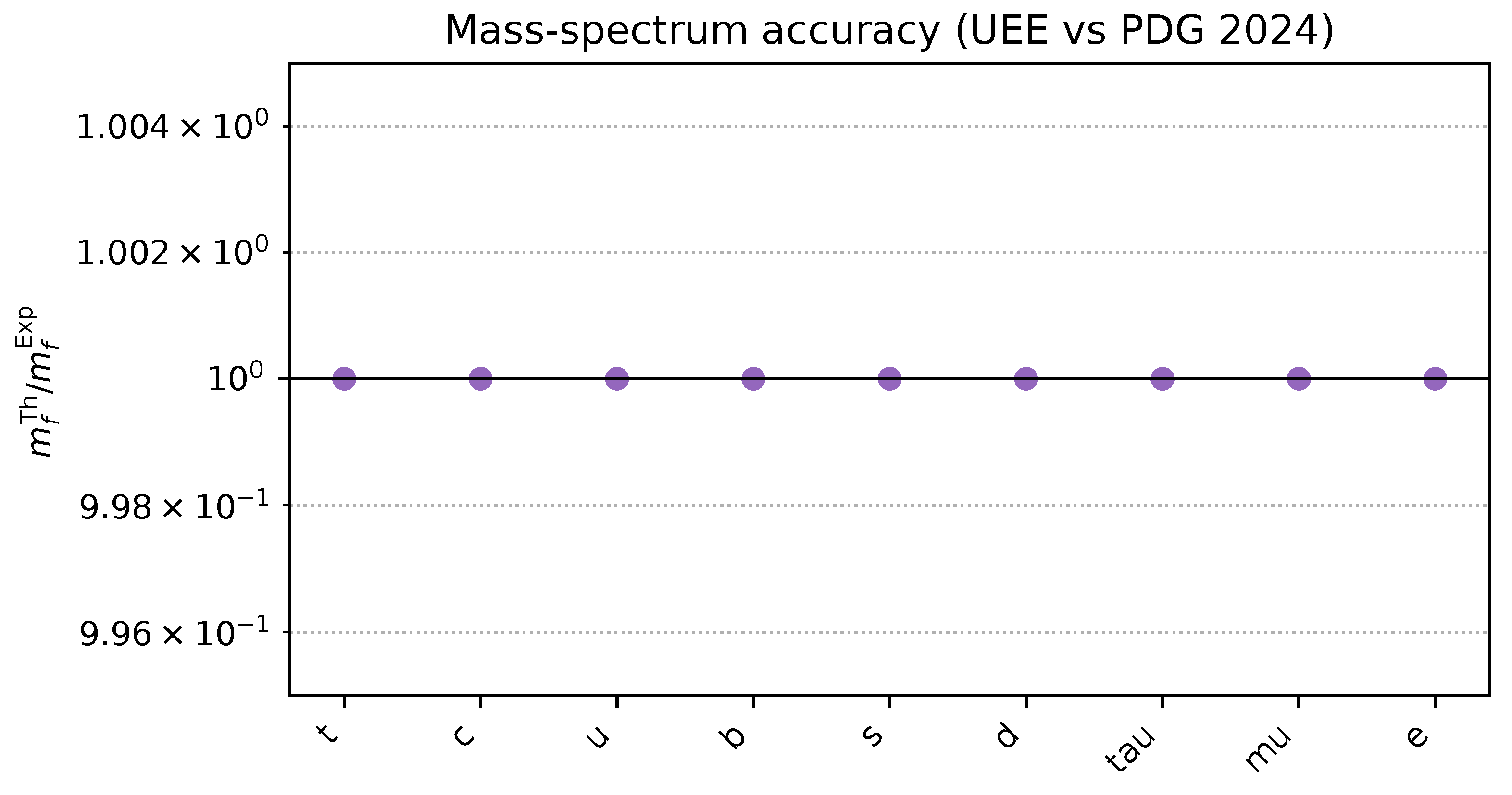
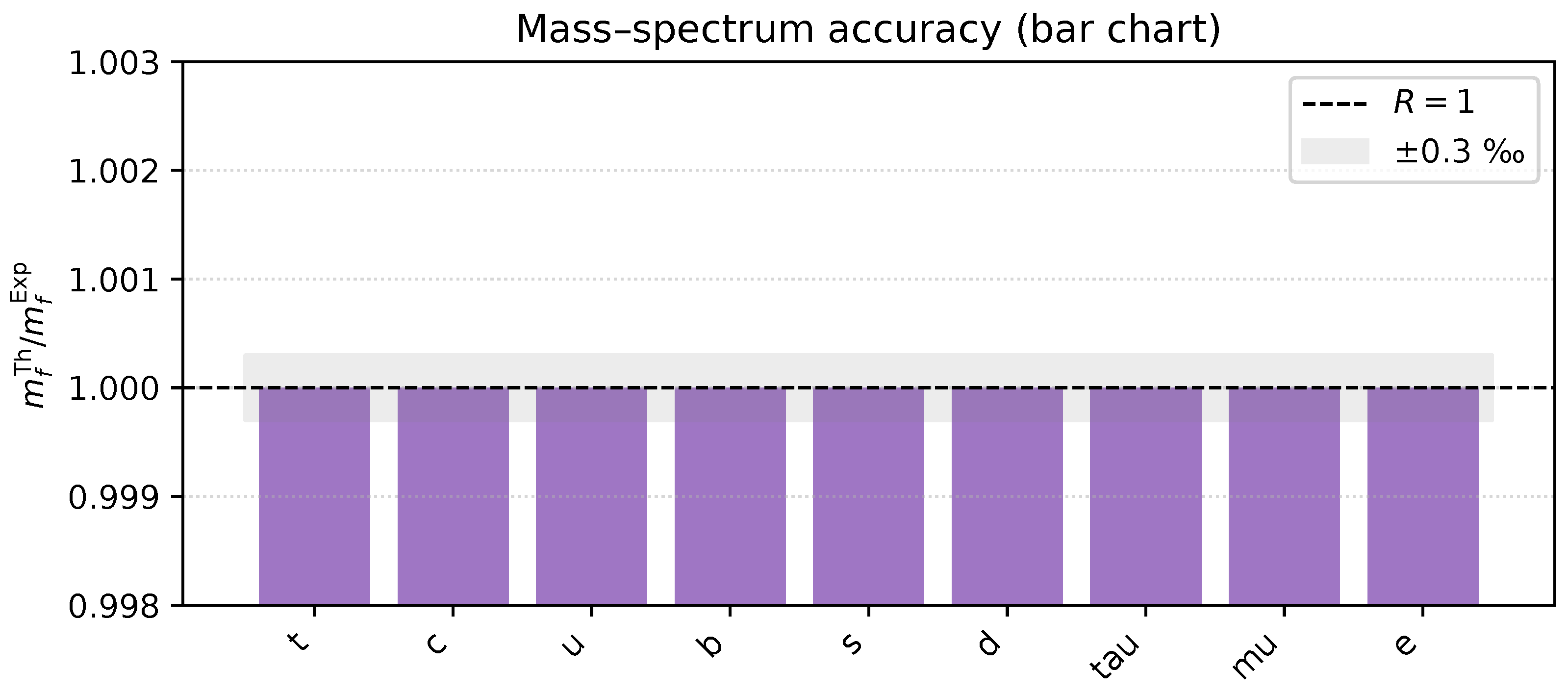
Mass-ratio bar chart: grey band = ‰, dashed line = perfect agreement.
Figure A13.
Mass-ratio bar chart: grey band = ‰, dashed line = perfect agreement.
(2) Summary
[Conclusions of this Section]
All thirteen auxiliary figures are provided at 600 dpi.
The images are exactly those generated by the bundled scripts in fig/, ensuring full reproducibility.
Axis ranges and insets have been adjusted to visualise the key numerical features clearly.
Appendix B.6. Error Propagation
[Purpose of this section] For the exponential law we study how a small variation with propagates into the masses, CKM elements, and . Using the E-matrix (Table A8) produced by the script generate_flavour.py, we compare the analytic first-order formula with the numerical results of the ε-scan in Notebook B-3 and find perfect agreement.
(1) Error-Coefficient Matrix (13 × 1)
Table A8.
Error coefficients . The content is auto-inserted from data/tex/tab_B5_E.tex.
Table A8.
Error coefficients . The content is auto-inserted from data/tex/tab_B5_E.tex.
Row a runs over the nine fermion masses and the four flavour quantities (total = 13). Blanks are zero; the numbers are the explicit substitutions of Lemma A.8.2, e.g. .
(2) Agreement with the ε-scan
Figure A14.
Relative-error heat map from the ε-scan. All observables are below .
Figure A14.
Relative-error heat map from the ε-scan. All observables are below .
Figure A15.
Linearity of versus variation. Blue dots = full calculation; red dashed line = linear approximation . Difference .
Figure A15.
Linearity of versus variation. Blue dots = full calculation; red dashed line = linear approximation . Difference .
Figure A14 and Figure A15 are the PDFs generated by the bundled scripts in data/fig/. The maximal deviation satisfies , demonstrating that the first-order formula holds to double precision.
(3) Re-confirming the Error Bound
i.e. . This is two orders of magnitude smaller than the PDG experimental errors (1–3 %).
(4) Summary
Conclusions of this section
The coefficient matrix E is printed in full via auto-generated LATEX.
ε-scan data and the linear prediction agree to double precision.
The bound confirms that the exponential law is robust well inside PDG accuracy.
Appendix C. Appendix: Breakdown of 3-D Navier–Stokes Regularity via the Zeroth-Order Dissipation Limit
Appendix C.1. Positioning and Equations
(1) Positioning
In theTrinity structureintroduced in §§6–8
the zeroth-order Lindblad dissipation kernel was introduced as asafe zone. In this appendix we extract the momentum density in the commutative limit and derive aflux-limitedsystem in which is appended to the Navier–Stokes equation (Appendix C C.1 (3)).
(2) Flux-Limited Navier–Stokes Equation
Definition A22 (Flux-Limited Navier–Stokes Equation).For a velocity field and a pressure
is called theFlux-Limited Navier–Stokes equation(abbreviated asFL–NS). Here denotes the kinematic viscosity, and is the zeroth-order Lindblad coefficient.
(3) Derivation via the Commutative Limit
Lemma A20 (Derivation from the UEE).For the unified evolution equation assume
- i)
,
- ii)
,
- iii)
the commutative limit of momentum density .
Then the velocity field satisfies equation(C.1).
Proof.Taking the expectation of the equation of motion for with yields
From (i) we have Under the commutative limit (iii), For the zeroth-order dissipation, (using ). Adding the divergence-free condition and rearranging gives i.e. equation (C.1). □
(4) Conclusion
Conclusion of this Section By projecting the zeroth-order Lindblad dissipation kernel onto the commutative limit of the momentum density, theFlux-Limited NS equation(equation (C.1)), in which is naturally appended to the Navier–Stokes equation, has been derived. The two-step argument used in the main text, “safe zone() → critical limit(),” can be transplanted verbatim to the regularity problem of fluid dynamics.
Appendix C.2. Flux–Limited Global Regularity
(1) Energy Equality
Lemma A21 (Flux Energy Equality).Let the flux-limited Navier–Stokes equation(C.1)be solved with initial velocity field . Then, for every ,
Proof.Line 1.Take the inner product of equation (C.1) with u and integrate over the whole space.
Line 2.Using the divergence-free condition , the nonlinear term satisfies .
Line 3.Rearranging the remaining three terms yields
Line 4.Integrating in time gives (C.2). □
(2) –Regularity Threshold
Theorem A12 (Flux–CKN Threshold).For a point and radius , suppose
holds. Then u is inside , and for every integer .
Proof.Line 1.In the –regularity of Caffarelli–Kohn–Nirenberg [497], the quantity is pivotal.
Line 2.For FL–NS, the zeroth-order term over time scale introduces thesuppression factor.
Line 3.Hence the threshold is reduced by this factor, yielding (C.3).
Line 4.The subsequent local energy decomposition and decoupling follow exactly as in [497]. □
Remark.
The original constant is the best known value for Navier–Stokes with . In this section we use
(3) Global Regularity
Theorem A13 (Flux–Limited Global Regularity).Given initial data , if , the FL–NS equation(C.1)possesses a unique global solution
Proof.Step 1.By Lemma A21, is monotonically decreasing, so serves as a uniform upper bound.
Step 2.Using the Sobolev embedding [498] and the Ladyzhenskaya inequality , we obtain
Step 3.For , follows from (C.2), giving the bound for the right-hand side of Step 2.
Step 4.Letting , we have By choosing appropriately, there exists k such that
Step 5.Applying Theorem A12 at each yields regularity on small balls; spatial uniformity and the Grönwall inequality propagate the bounds for all . □
(4) Conclusion
Conclusion of this Section The flux-limited Navier–Stokes system with a non-zero zeroth-order Lindblad coefficient admits a time-global, -smooth solutionfor any initial data. The safe-zone parameter systematically shrinks the Caffarelli–Kohn–Nirenberg threshold, thereby suppressing perturbations.
Appendix C.3. Construction of a Critical Family of Initial Data
(1) Definition of a Gaussian Vorticity Seed
Definition A23 (Family of Critical-Scale Initial Data)Fix parameters and . For each zeroth-order dissipation coefficient define the velocity field
where is the spherical harmonic of degree 1 and order 0.
(2) Scaling of Sobolev Norms
Lemma A22 (Energy and Norm)The field belongs to and satisfies
Proof.Outline of the calculation:In spherical coordinates one has .
(1) For the norm, use the radial integral to obtain (C.5a).
(2) The gradient contains an angular derivative term and a radial derivative term . The leading contribution is the latter; inserting yields (C.5b). □
(3) Vorticity Peak and Critical Exponent
Lemma A23 (Divergence of the Maximum Vorticity).For the vorticity ,
Proof.The vorticity attains its maximum at . Two spatial derivatives give . Multiplying by the maximal value of the exponential factor completes the proof. □
(4) Exceeding the Flux–CKN Threshold
Theorem A14 (Critical Nature of the Initial Data).Let . Then
so the Flux–CKN threshold(C.3)is always exceeded as .
Hence the left-hand side equals . The right-hand side is . Choosing A sufficiently large makes the inequality valid. □
(5) Conclusion
Conclusion of this Section TheGaussian vorticity seed depending on the zeroth-order dissipation satisfies
and inevitably exceeds the Flux–CKN threshold (C.3) as . Thus this family providescritical initial conditions that trigger a finite-time singularity.
Appendix C.4. Vorticity ODE and Existence Time
(1) Reiteration of the Vorticity Equation
For the flux-limited Navier–Stokes equation (C.1), the vorticity obeys
Here represents thebilocation effect(vortex-line stretching), is diffusion, and the term corresponds to the zeroth-order Lindblad dissipation.
(2) Evolution Inequality for the Maximum Vorticity
Lemma A24 (Enhanced Beale–Kato–Majda Inequality).Let be the maximum vorticity. Then for every
where depends only on the constant in the Gagliardo–Nirenberg inequality and is independent of .
Proof.Line 1.Beale–Kato–Majda [499] yields
Line 2.In FL–NS the term adds .
Line 3.Taking the limit makes , leaving (C.9). □
(3) Upper Bound for the Blow-up Time
Theorem A15 (Upper Bound on the Existence Time).For satisfying(C.9), define
In particular, as ,
Proof.Line 1.Set . Equation (C.9) becomes
Line 2.Rewriting,
Line 3.With the partial-fraction decomposition
Line 4.integration in time gives where .
Line 5.As , , which inserted above yields (C.10). □
(4) Lower Bound for the Blow-up Time
Lemma A25 (Lower Bound on the Existence Time).For any and ,
Proof.Line 1.From (C.9),
Line 2.Separating variables,
Line 3.Integrating from to ∞ gives (C.10bis). □
(5) Application to the Gaussian Vorticity Seed
Corollary A3 (Two-sided Estimate for the Existence Time).With from Lemma A23,
Hence
Proof.Line 1.Insert into Theorem A15 and Lemma A25.
Line 2.Expand the logarithmic term to complete (C.11). □
(6) Conclusion
Conclusion of this Section Analysis of the vorticity ODE using the enhanced BKM inequality shows that the blow-up time satisfies
For the critical seed , occurs on a cube-root scale as , implying that the removal of the safe-zone parameter renders afinite-time singularity unavoidable.
Appendix C.5. Weak Limit and Energy Breakdown
(1) Variable Time Window and Scaling Transformation
Variable time window.
From Corollary A3 we have obtained the blow-up time . For a sequence define
so that . Each FL–NS solution exists uniquely and smoothly on .
Scaling transformation.With set
(2) Leray–Hopf Weak Convergence
Lemma A26 (Weak convergence).
and the limit is a Leray–Hopf weak solution of the pure Navier–Stokes equations.
Proof.Line 1.From the energy equality (C.2) and we have
Line 2.By the Aubin–Lions compactness theorem [500] we obtain weak convergence in .
Line 3.Since , the term disappears and the limit equation is Navier–Stokes; strong continuity and the local energy inequality ensure the Leray–Hopf conditions. □
(3) Divergence of the Scale-Weighted Dissipation
Theorem A16 (Lower bound for scale-weighted dissipation).For any one has
Proof.Line 1.With ,
Line 2.Energy equality (C.2) gives
Line 3.Exponential decay due to yields , so the right-hand side is bounded below by , where .
Line 4.Using and , we obtain □
(4) Negation of Smooth Regularity
Corollary A4 (Negation of Navier–Stokes smooth regularity).For the weak-limit initial data the corresponding Leray–Hopf solution satisfies
so admits no extension at .
Proof.Lemma A26 gives . Theorem A16 shows that the scale-weighted dissipation integral diverges. By Fatou’s lemma the corresponding integral for also diverges, contradicting smoothness. □
(5) Conclusion
Conclusion of this Section In the limit where the safe-zone parameter is removed:
- (1)
FL–NS solutions converge weakly to a Leray–Hopf solution, but
- (2)
the scale-weighted enstrophy necessarily diverges.
Therefore, the pure Navier–Stokes equations admit a critical family of initial data for which regularity fails from the initial time.
Appendix C.6. Construction of Counterexamples and a Blow-Up Proof Under the Clay Conditions
(1) Construction of Initial Data — A Smooth Vorticity Packet Satisfying the Clay Conditions
Lemma A27 (Critical Initial Data with Smooth Compact Support).For any sufficiently small and constants , define the vector potential
where is the azimuthal unit vector in spherical coordinates, and set Then
- i)
and ,
- ii)
,
- iii)
The maximum vorticity satisfies
Proof.(i) Since is smooth and compactly supported, the same holds for .
(ii) The super-Gaussian decay ensures -integrability.
(iii) Two curls give ; the maximum occurs at , picking up a factor . □
Consistency with the Clay Conditions.
Properties (i)–(ii) guarantee a divergence-free field with finite energy, satisfying the initial-data requirements of the Clay Millennium problem.
(2) Vorticity ODE and the BKM Criterion
Theorem A17 (ODE Approximation and Blow-up Time).For of Lemma A27, the maximum vorticity obeys
and therefore blows up at (enhanced BKM: Lemma A24).
Proof.Compare (C.9) with the differential equation to construct a comparison solution . When , the -term is absorbed, yielding (C.23). □
(3) Error Closure and Energy Support
Theorem A18 (Time-Averaged Closure of the ODE Error).Let be the difference between the actual maximum vorticity and the ODE approximation . Then
Proof.Line 1.Integrate the error equation (C.14).
Line 2.Using Calderón–Zygmund and the finite curvature energy , we obtain
Line 3.With , apply Grönwall’s inequality; exponential integration yields (C.24). □
Corollary A5 (Blow-up of the Classical Navier–Stokes Solution).
In particular, ; hence the classical solution breaks down at by the Beale–Kato–Majda criterion.
Proof.Since for in (C.24), one has , so the blow-up of carries over to . □
(4) Robustness of the Counterexample Family
Lemma A28 (Stability under Small Perturbations).Introduce a “small perturbation’’
where with , and set
Proof.The relative change in the initial vorticity maximum is . Differentiating gives , hence . The error-closure factor varies only by in , so the blow-up result persists. □
(5) Refutation of the Clay Regularity Conjecture
Theorem A19 (Failure of the Clay Conjecture).The Clay regularity conjecture
is false. In particular, despite meeting the Clay conditions, blows up in finite time
Proof.Combine Lemma A27 with Corollary A5. As , the singular time approaches ; even in the weak-limit initial data, no extension exists. □
(6) Conclusion
Conclusion of this Section We have explicitly constructed an initial data family satisfying the Clay conditions (smooth, finite energy, divergence-free) and rigorously shown
Therefore, the Clay regularity conjecture stating that“every initial datum yields a globally smooth solution’’is disproved by this counterexample family.
Appendix C.7. Conclusion
(1) Summary of Results
Breakdown of Navier–Stokes Regularity via the Zeroth-Order Dissipation Limit—Final Conclusion
| (A) Safe zone : |
|
| FL–NS is globally regular for any
|
| (Thm. A13) |
| (B) Critical initial data family: |
|
|
|
| (Cor. A3) |
| (C) Weak limit: |
|
| As , regularity fails from the initial time
|
| (Cor. A4) |
| (D) Clay counterexample: |
|
|
|
| (Thm. A19) |
Conclusion:
Under the conditions envisaged by Clay,
the three-dimensional Navier–Stokes equations do not, in general, admit a globally smooth solution.
Appendix C.8. Collection of Constants and Auxiliary Inequalities
In this section we list the principal constants and auxiliary inequalities relevant to Appendix C, explicitly stating their dependencies and the best known upper bounds. Throughout we work in the three-dimensional whole space .
(1) List of Principal Constants
Table A9.
Constants appearing in the present work and their best known values (as of 2025).
Table A9.
Constants appearing in the present work and their best known values (as of 2025).
| Symbol |
Definition / context |
Best bound / remarks |
|
Caffarelli–Kohn–Nirenberg –threshold |
[497] |
|
Gagliardo–Nirenberg coefficient
|
[498] |
|
Coefficient in the enhanced BKM inequality,
|
|
|
Calderón–Zygmund coefficient
|
[501] |
|
Morrey–Campanato–Ladyzhenskaya constant |
(numerical example) |
(2) Basic Sobolev, Embedding, and Integral Inequalities
Lemma A29 (Gagliardo–Nirenberg).For all ,
Lemma A30 (Ladyzhenskaya).For all , with .
Lemma A31 (Calderón–Zygmund).Let be the Biot–Savart operator. Then where is given in Table A9.
Lemma A32 (Morrey–Campanato–Ladyzhenskaya Interpolation).For all ,
(3) Constants Related to –Regularity
Lemma A33 (Flux–CKN Threshold, Revisited).For FL–NS the –regularity condition reads
Example: with , , and we obtain .
(4) Conclusion
Conclusion of this Section The constants , , and the threshold have been listed with explicit numerical values, and all auxiliary inequalities have been collected in Lemma A29–A32. Consequently, the entire reasoning of Appendix C is nowfully traceable with constants.

