
Submitted:
13 May 2025
Posted:
15 May 2025
You are already at the latest version
Abstract
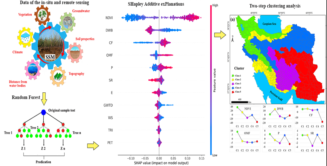
Understanding the impacts of spatial non-stationarity of environmental factors on surface soil moisture (SSM) in different seasons is crucial for effective environmental management. Yet, our knowledge of this phenomenon remains limited. To fill this gap, we have introduced a framework combining the model agnostic SHapley Additive exPlanations (SHAP) technique with a two-step clustering analysis to provide spatial interpretations for machine learning models. Due to spatial and temporal limitations of in-situ SSM data in Iran, we evaluated the performance of global daily datasets, including SMAP, MERRA-2, and CFSv2, from 2015 to 2023 using the agrometeorological stations to select the best dataset for the machine learning process. Subsequently, SSM values were calculated for Iran’s 609 catchments using the most optimal dataset. Furthermore, we selected a set of climatological, hydrological, topographical, vegetation, and soil factors influencing SSM. While Random Forest (RF) was employed to estimate SSM, the SHAP technique was used for RF spatial interpretation in conjunction with the two-step cluster analysis. The results revealed that among the datasets, SMAP exhibited the highest median correlation and the lowest median root mean square error when compared to in-situ stations. Findings indicated that the RF model can offer SSM estimates with R2 values of 0.89, 0.83, 0.70, and 0.75 for the winter, spring, summer, and autumn seasons, respectively. The results of SHAP and two-step clustering demonstrated that climatic factors primarily influence winter and autumn SSM. In contrast, in spring and summer, SSM is predominantly affected by vegetation and soil characteristics. These findings provide valuable reference points and policy recommendations for effectively managing SSM in various catchments.
Keywords:
surface soil moisture dynamics
; Machine Learning
; random forest
; SHapley Additive exPlanations
; environmental factors
1. Introduction
Surface soil moisture (SSM) influences climate processes by governing the distribution of precipitation into runoff, evapotranspiration, and infiltration, as well as by affecting the partitioning of incoming energy into latent and sensible heat fluxes (Seneviratne et al., 2010; Zhang et al., 2021; Han et al., 2023). SSM also plays a crucial role in the global hydrological cycle and understanding water resource management, flood generation, and climate changes at local and global scales (Sure and Dikshit et al., 2019; Yang et al., 2024). The significance of SSM becomes more pronounced in dry and semi-arid regions, where water scarcity is a prominent concern (Schwinning and Sala, 2004; Cosh et al., 2008). In these regions, changes in SSM can lead to a cascading effect, affecting the rates of groundwater recharge (Chen and Hu, 2004; Parizi et al., 2020), vegetation dynamics (D'Odorico et al., 2007), and regional climate patterns (Seneviratne et al., 2010). Hence, precise monitoring and prediction of SSM and the investigation of factors affecting it are indispensable for sustainable water resource management, risk assessment, and mitigation associated with drought and other hydrometeorological hazards in these regions (Cai et al., 2019; Lagos et al., 2020; Nikraftar et al., 2021a).
However, one significant bottleneck in SSM monitoring, particularly in arid and semi-arid regions, is the scarcity of high-quality and reliable in-situ data (Gruber et al., 2013; Everson et al., 2017; Rasheed et al., 2022). While in-situ sensors provide localized, high-quality measurements, their geographic coverage is often limited due to financial, logistical, and accessibility constraints (Xu et al., 2021a). In many countries, particularly those with vast arid and semi-arid regions, installing and maintaining in-situ networks is challenging (Gruber et al., 2013; Everson et al., 2017; Dorigo et al., 2021). Thus, validating global SSM datasets with in-situ measurements is becoming increasingly important (Jamei et al., 2020). Country-specific validation of these global datasets allows for the calibration of models to regional conditions, enhancing their reliability and applicability for resource management strategies (Dorigo et al., 2021; Guevara et al., 2021).
Understanding the factors that influence SSM is key to effective monitoring and management (Xu et al., 2021b; Rasheed et al., 2022). SSM is influenced by many factors such as precipitation (Cho and Choi, 2014; Fu et al., 2022), texture and organic matter content of soil (Cosby et al., 1984; Jawson and Niemann, 2007; Wang and Franz, 2015; Han et al., 2023), topography (Perry and Niemann, 2007), vegetation (Jiang et al., 2008), and groundwater (Meng et al., 2022). Seasonal trends, land-use changes, and evapotranspiration rates are also critical elements affecting SSM dynamics (Jung et al., 2010; de Queiroz et al., 2020). Understanding these variables and their interactions is vital for developing strategies for SSM management, particularly in arid and semi-arid regions where each drop of water counts (Wang et al., 2019). Insight into these factors can improve the precision of hydrological models and contribute to the development of adaptive management strategies for water resources (Grayson et al., 1997).
The advent of machine learning techniques has opened new avenues for hydrological modelling, particularly in the exploration of complex, non-linear relationships among factors influencing SSM (Grayson et al., 1997; Ali et al., 2015; Boueshagh and Hasanlou, 2019; Adab et al., 2020). Machine learning models can handle large datasets and account for complex interactions, thereby offering a more nuanced understanding of hydrological processes (Ahmad et al., 2010). Machine learning techniques such as Random Forest, Support Vector Machines, and Neural Networks have shown promise in hydrological applications, including SSM prediction and classification (Carranza et al., 2021). Nevertheless, numerous water scientists hesitate to adopt machine learning techniques due to their perceived "black box" nature, as they make it challenging to grasp how the model leverages input variables for prediction (Wang et al., 2022). Recently, SHapley Additive exPlanations (SHAP), a model-agnostic game-theoretic approach, has found successful application in the interpretation of machine learning models (Lundberg and Lee, 2017; Liu et al., 2022). Unlike conventional methods that only quantify the influence of input variables on the model output, SHAP can reveal whether each variable exerts a positive or negative impact on the model (Wang et al., 2022).
While previous research has utilized factors that influence SSM and employed machine learning algorithms for estimation (e.g., Carranza et al., 2021; de Oliveira et al., 2021), most studies focus on specific hydrologic conditions or operate within a limited catchment scale, resulting in models with confined applicability. The lack of diverse, large-scale data and the limited scope of prior research mean that we are yet to develop models that are broadly applicable across different hydro-climatic conditions. On the other hand, due to the spatiotemporal variability in SSM, it's crucial to understand how spatial non-stationarity of pivotal environmental factors affects SSM across different seasons. To fill this gap, we introduce a framework that combines the model-agnostic SHAP technique with a two-step clustering analysis to provide spatial interpretations for machine learning models in Iran’s 609 catchments with diverse hydro-climatic conditions. These spatial interpretations can provide guidance and policy recommendations for the effective management of SSM within 609 various catchments across Iran.
2. Materials and Methods
2.1. Study Area
Iran with an area of approximately 1,648,195 km2 is located in the Middle East and faces challenges related to water resource scarcity (Nikraftar et al., 2023). Iran is typically characterised by an arid and semi-arid climate, with an average annual precipitation of approximately 250 mm (Rahmani et al., 2016). As indicated by climate classification (Figure 1), a significant portion of the country falls under the category of a warm-dry climate, naturally resulting in SSM deficits (IMO, 2019). In recent years, SSM deficits in Iran have been exacerbated by factors that include climate change, excessive groundwater extraction, mismanagement of surface water, and inefficient irrigation practices (Ashraf et al., 2021). Such SSM shortages can lead to detrimental environmental consequences, including desertification, soil degradation, dust storms, wind erosion, and the degradation of air and water quality (Sivakumar and VStefanski, 2007). Therefore, it is imperative to monitor SSM and to study the factors influencing it in Iran to ensure effective environmental management (Gheybi et al., 2019; Jamei et al., 2020). Nonetheless, SSM remains inadequately monitored in numerous regions of Iran, and the existing measurements (as depicted in Figure 1) lack sufficient temporal and spatial resolution (Rahmani et al., 2016).
Under these circumstances, remote sensing data can offer a viable solution for monitoring SSM in Iran (Ranjbar Saadatabadi et al., 2021). Consequently, it is essential to validate and assess global SSM products using in-situ stations to gauge their real-world effectiveness before using them across all climatic regions in Iran. In this study, after validation of the SSM products, the environmental factors affecting SSM were investigated across 609 catchments in Iran. The total drainage area of these catchments is 1,648,195 km2 (IWRMC, 2023). These catchments are distributed across diverse climates, spanning from cold-dry to warm-humid, as illustrated in Figure 1. They exhibit different topographic characteristics, geological compositions, soil varieties, and vegetation, leading to diverse hydrological conditions throughout the country. Additionally, the land cover map obtained from ESA (ESA-World Cover, 2020) with a 10 m resolution reveals that bare/sparse vegetation, grasslands, croplands, and forests constitute the predominant land cover in the studied catchments, accounting for 64.2%, 18.9%, 11.8%, and 1.70%, as given in Table S1. Therefore, validating SSM products through in-situ stations and utilising an appropriate dataset to investigate the environmental factors affecting SSM in this diverse environment facilitates the advancement of sustainable SSM management practices.
2.2. Datasets
2.2.1. SSM Data
The in-situ SSM data from agrometeorological stations were gathered from the Iran Meteorological Organization, IMO (IMO, 2023) for the period spanning February 1, 2006, to March 31, 2023. Unfortunately, SSM data is not widely available in numerous regions of Iran and have several gaps (Rahmani et al., 2016; Gheybi et al., 2019). Hence, a total of 42 stations were chosen throughout Iran, distributed as follows: 13 stations in cold-dry climates, 2 in cold-humid, 11 in warm-dry, 3 in warm-humid, 8 in moderate-dry, and 5 in moderate-humid (Figure 1). Considering previous studies (e.g., Colliander et al., 2017; Xu, 2021a; Tian & Zhang; 2023), here we utilized three primary SSM datasets, namely Soil Moisture Active Passive (SMAP), Modern-Era Retrospective analysis for Research and Applications, Version 2 (MERRA-2), and Climate Forecast System, Version 2 (CFSv2), to validate SSM at a depth of 0-5 cm using in-situ data (Table 1).
The SMAP satellite mission by NASA was launched on January 31, 2015, to globally map soil moisture and the freeze/thaw state of landscapes (Wu et al., 2020). While the satellite initially utilized both an L-band radar and an L-band radiometer, the radar instrument encountered a failure after approximately 11 weeks of operation, and the production of soil moisture data continues using only the radiometer data (Colliander et al., 2017). SMAP measurements provide direct sensing of SSM in the upper 5 cm of the soil (Kimball et al., 2018; Xu et al., 2021). In this study, we employed the SMAP Level 4 passive product (Reichle et al., 2019), which features a spatial resolution of 9 km (Table 1).
MERRA-2, generated by NASA Global Modeling and Assimilation Office (GMAO), stands as the most recent atmospheric reanalysis covering the modern satellite era, offering global reanalysis data spanning from 1980 to the present (Gelaro et al., 2017). Reichle et al. (2017) validated MERRA-2 against in-situ measurements in North America, Europe, and Australia, demonstrating that its performance is slightly superior to that of ERA-Interim/Land. In this study, we utilised MERRA-2, which featured a spatial resolution of 56 km by 70 km (Table 1). CFSv2 was made operational at the National Centers for Environmental Prediction (NCEP) in March 2011 (Saha et al., 2014; Dirmeyer and Halder; 2016). The soil moisture dataset within the CFSv2 encompasses four layers (at 5, 25, 70, and 150 cm depths) and boasts a spatial resolution of approximately 22 km (Saha et al., 2011). It's worth mentioning that while SMAP directly measures SSM, MERRA-2 and CFSv2 rely on model-based reanalysis data generated through physical models, observations, and data assimilation. These three SSM datasets were resampled to 0.25º × 0.25º by bilinear interpolation (Xu et al., 2021) to ensure consistency across the datasets.
2.2.2. Factors Influencing SSM
We selected the candidate factors that influence SSM based on previous studies (e.g., Chen et al., 2004; Patel et al., 2009; Zhao et al., 2017; Raduła et al., 2018; Han et al., 2023) and data availability (Table 2, Figure S1). We used the catchment-averaged monthly data of the following parameters: precipitation, potential evapotranspiration, solar radiation, wind speed, normalized difference vegetation index (NDVI), and groundwater table depth. Additionally, time-invariant catchment attributes such as, distance from water bodies, clay fraction, organic matter fraction, elevation, and topography roughness index were included (Table 2). The mean monthly precipitation for the studied catchments was computed using the Radial Basis Function (RBF) interpolation method (Du, 2008) in Python. This was based on daily precipitation data collected from 422 synoptic stations between 2015 and 2023 from IMO (IMO, 2023). The mean monthly potential evapotranspiration for the studied catchments was determined using MODIS global evapotranspiration product (i.e., MOD16A2, Running et al., 2017) at a 500 m resolution.
Solar radiation and wind speed data were obtained from the ERA5-Land dataset (Muñoz-Sabater et al., 2021) at a spatial resolution of 11 kilometers, while an analysis of vegetation dynamics was conducted using the NDVI index and Sentinel-2 data (Copernicus, 2023) with 10 m resolution. The NDVI proves to be a suitable index for detecting vegetation changes, particularly within arid and semi-arid regions (Parizi et al., 2021). To generate a time series of groundwater table depth, we utilised monthly data from 11,003 observation wells collected by the Iran Water Resources Management Company (IWRMC, 2023). We derived the average monthly groundwater table depth for each catchment using the RBF interpolation method. The mean distance of each catchment from water bodies was determined by utilising the water bodies' data (NOAA, 2023) and the Euclidean Distance method in ArcGIS (ESRI, 2013). The SoilGrids250m dataset (Hengl et al., 2017) was employed to extract the clay and organic matter fractions within the upper vadose zone. Finally, we calculated the mean elevation and topography roughness index for the studied catchments using an ALOS DEM with a 30 m resolution (Tadono et al., 2016) and Focal Statistics tools in ArcGIS. All factors influencing SSM were extracted using the Google Earth Engine platform (Amani et al., 2020), Python and ArcGIS software. Additional details regarding the factors influencing SSM and their correlation are provided in the supplementary material.
2.3. Methods
2.3.1. Statistical Metrics
The performance of global SSM products was assessed using the Root Mean Squared Error (RMSE), Relative Bias (RBias), Kendall’s Tau (τ), and Kling-Gupta efficiency (KGE′) (Tang et al., 2020; Saemian et al., 2021; Fahrudin et al., 2020; Parizi et al., 2022):
where N represents the number of samples, Ref is the reference values (i.e., in-situ data), and Tar is the target values (i.e., SMAP, MERRA-2, and CFSv2 data) for each record (i). Furthermore, we utilized the KGE′ statistic, initially introduced by Gupta et al. (2009) and subsequently modified by Kling et al. (2012). KGE balances the contributions of correlation, bias and variability terms as follows (Tang et al., 2020):
where r represent the correlation coefficient between Ref and Tar datasets, γ is the variability ratio, β is the bias ratio, μ is the mean SSM, CV is the coefficient of variation, and represents is the standard deviation. The better values have higher KGE (Saemian et al., 2021).
2.3.2. Random Forest
The Random Forest (RF) model was initially introduced by Leo Breiman in 2001 (Naghibi et al., 2016). The RF algorithm does not necessitate any alterations, conversions, or modifications to the input data, and it autonomously handles missing values (Breiman et al., 2012; Pouyan et al., 2021). An RF model comprises a multitude of decision trees designed to be as uncorrelated as possible (Kaiser et al., 2022). To create an uncorrelated collection of trees, the RF employs bagging and feature randomisation during the construction of the decision trees. This implies that each tree is trained on a random sample drawn from the training set with replacement, a technique known as bootstrapping (Amini et al., 2022). Additionally, each tree is limited to a random subset of the available features (Breiman, 2001).
One of the advantages of the RF method, as highlighted by Tyralis et al. (2019), is that it yields consistent predictions while diminishing variance without augmenting prediction bias. In this study, we used the RandomForestRegressor from the machine learning library sklearn (Pedregosa et al., 2011; Buitinck et al., 2013) for the Python programming language. For enhanced convergence speed and to mitigate the impact of local extremes on training, the input variables undergo normalization to a range of 0.1 to 0.9 before the training process. As some models encounter issues when normalized between 1 and 0, we chose to normalize the input variables using the adjusted min-max method within the range of 0.1 to 0.9 (Gökhan Aksu et al., 2019).
The hyperparameters were tuned using a 10-fold cross-validation approach on the training set. This involved dividing the training set into ten subsets, with one-tenth serving as the test sample in each fold, while the remaining data was employed for constructing the regression trees. In each fold, the test sample comprised randomly selected points from the overall training set that had not been included as a test sample in previous folds. The comparison of RMSE values for each hyperparameter combination across the 10-fold cross-validation provided an assessment of model performance (Carranza et al., 2021). To maintain a distinct validation set, a cross-validation scheme is a precaution against model overfitting (Lever et al., 2016; Kaiser et al., 2022). We employed a random selection process for the training dataset to allocate 80% of the data for training purposes, while the remaining 20% was reserved for testing.
2.3.3. SHAP
SHAP method represents a model-agnostic game-theoretic technique for interpreting machine learning models (Lundberg and Lee, 2017). Unlike conventional methods that only quantify the influence of input variables on the model output, SHAP can disclose whether each variable exerts a positive or negative impact on the model (Wang et al., 2022). In other words, SHAP can analyse an individual prediction by considering it as a composite result of the combined effects of each input variable on the output value (i.e., the predicted value). This approach allows users to gain insight into the magnitude of influence and how each input variable affects the output value (Lundberg and Lee, 2017, Broeck et al., 2022). Using a pre-trained machine learning model denoted as M and a set of input variables x={x1, …, xq}, SHAP employs an explanation model E to ascertain the individual influence of each variable on the behaviour of model M (Liu et al., 2022). SHAP express as:
where q represents the number of input variables, t is the variable simplification, ɸi ∈ R represents the contribution of each variable to the machine learning model, and \ is the difference-set notation for set operations (Wang et al., 2022; Liu et al., 2022). In this study, the Python SHAP library was employed to assess feature importance in conjunction with the RF model.
2.3.4. Cluster Analysis
A two-step cluster analysis was conducted on the outcomes of the SHAP model to enhance our spatial understanding of the effects of factors influencing SSM within the studied catchments. In other words, employing a two-step cluster analysis can offer spatial interpretations for the factors that affect SSM, utilizing the outcomes generated by RF and SHAP. We follow the methodology for the two-step cluster analysis outlined by Fahy et al. (2019). Only a summary of the technique is provided here, and rather, the reader is directed to Fahy et al. (2019) for a detailed description of the approach. The method involves two steps: (1) whole records are probed by distance to construct a classification tree, whereby records in the same tree node are most similar (Qin et al., 2019); (2) nodes are classified using the cohesion technique and clustering results are evaluated using the Bayesian information criterion (BIC) or the Akaike information criterion (AIC), which determine the structure of the final cluster (Chiu et al., 2001; Satish & Bharadhwaj, 2010).
3. Results and Discussion
3.1. Performances of SSM Products
Figure 2 shows the SSM validation results based on 42 in-situ stations from April 2015 to March 2023. The findings suggest that among the evaluated datasets, SMAP stands out with the highest median values for τ and KGE (0.740 and 0.690), and it also exhibits the lowest median values for RMSE and RBias (0.068 and 0.030). Following SMAP, the MERRA-2 product demonstrates median values of τ and KGE at 0.684 and 0.604, along with median RMSE and RBias values of 0.085 and 0.034, respectively. CFSv2 shows the lowest median values for both τ and KGE (0.550 and 0.500), and it also has the highest median values for RMSE and RBias (0.113 and 0.059) among the three products, as shown in Figure 2. These findings demonstrate that SMAP outperforms the other datasets in estimating SSM in Iran.
The performance of SMAP aligns with the findings of the study conducted by Chen et al. (2018), which reported that SMAP has a global average anomaly correlation of 0.76. Xu et al. (2021a) evaluated eight global root zone soil moisture products (0-1 m depth) across the globe. Their findings indicated that SMAP, MERRA-2, JRA-55, and ERA-5 consistently showed a stronger correlation with in-situ root zone soil moisture measurements compared to GLDAS, NCEP R1, and NCEP R2. Colliander et al. (2017) validated SMAP SSM using core validation sites. They reported that the SMAP radiometer-based SSM product meets its expected performance, achieving an unbiased root mean square error of 0.04 m3 /m3 for volumetric SSM. It's noteworthy that global evaluations have not incorporated the in-situ SSM data from Iran.
There have been limited studies that have focused explicitly on evaluating SSM in Iran. These studies either concentrate on a particular local area, such as the Lake Urmia Basin (Maleki et al., 2019; Saeedi et al., 2021) or cover a short period in Iran (i.e., 2015-2016, as demonstrated in Gheybi et al., 2019). Additionally, some studies were solely concerned with validating a single product (e.g., Jamei et al., 2020, Jamei et al., 2022, and Amini et al., 2023). For example, Gheybi et al. (2019) validated SSM products from SMAP, SMOS, and AMSR2, using 23 in-situ stations in Iran from 2015 to 2016. Their results pointed to SMAP as the best-performing satellite-based product. Also, Jamei et al. (2022) stated that SMAP has a strong capacity for SSM data retrieval in Iran.
3.2. Spatial-Temporal Pattern of SSM
We calculated SSM for 609 catchments in Iran using the SMAP dataset, which demonstrated its optimality (Figure 3). Figure 3 illustrates the mean catchments-averaged daily SSM across 609 studied catchments from April 2015 to March 2023, delineated by different seasons and based on the SMAP dataset. The mean SSM for different seasons reveals distinct patterns, with winter having the highest median at 0.175 m3/m3, followed by spring at 0.160 m3/m3, while autumn and summer exhibit lower median of 0.096 m3/m3 and 0.081 m3/m3, respectively. These findings indicate notable seasonal variations in SSM within the studied catchments. Fakharizadehshirazi et al. (2019) stated that many catchments in Iran lack natural moisture, especially during the summer, leading to a heightened demand for irrigation in agriculture during this season. According to Garcia-Estringana et al. (2013), differences in soil moisture levels between dry (summer) and wet (winter) conditions are more pronounced in the upper surface layers (0–20 cm) when compared to deeper layers. Figure 3 also demonstrates that catchments with SSM exceeding 0.20 m3/m3 are predominantly located in northern, northwestern, western, and southwestern Iran, primarily within regions characterized by cold-humid and moderate-humid climates. In contrast, catchments with SSM below 0.05 m3/m3 are primarily concentrated in central and southeastern Iran that have warm dry climates.
3.3. SSM in Different Land Covers
Numerous studies have shown that changes in SSM exhibit varying characteristics when subjected to different land cover conditions (e.g., English et al., 2005; Jin et al., 2018; Feng et al., 2018; Zhou et al., 2023). The boxplots of SSM within the six primary land cover categories in Iran, as determined by the land cover map of ESA with a resolution of 10 m (ESA-World Cover, 2020) for the period spanning April 1, 2015, to March 31, 2023, are displayed in Figure 4a. The results reveal significant variations in median SSM across different land cover. Specifically, we found that forests exhibited the highest SSM with a median value of 0.180 m3/m3, followed by grasslands at 0.148 m3/m3, croplands at 0.148 m3/m3, shrubland at 0.117 m3/m3, built-up areas at 0.107 m3/m3, and bare/sparse vegetation at 0.093 m3/m3. Janani et al. (2022) studied SSM in various land-use patterns along the lower Bhavani River in India. They concluded that SSM is higher in forested areas compared to fallow land and built-up areas. Figure 4a also indicates that grasslands exhibit the highest soil moisture diversity, while bare/sparse vegetation shows the least diversity across Iran.
Figure 4b indicates a time series of SSM for various land cover in Iran, spanning from April 1, 2015, to March 31, 2023. The results show that in the early months of 2019, especially in March and April, SSM reached higher levels compared to the same months in the preceding and subsequent years (Figure 4b). The analysis of the precipitation time series in Iran (as shown in Figure 4b) for the years 2015-2023 reveals that the increase in SSM during those particular months is due to the increase in precipitation. This finding aligns with previous research. Nikraftar et al. (2021b) demonstrated that a significant increase in precipitation during the early months of 2019 led to a rise in the water level of Lake Urmia in northwestern Iran. Khosravi et al. (2020), Sadeghi et al. (2021), and Parizi et al. (2022) have documented that due to the heavy and unprecedented precipitation occurring between mid-March and April 2019, widespread flooding events affected 25 out of the 31 provinces in Iran. These events resulted in more than 77 human fatalities and inflicted approximately US$ 2.2 billion in damages.
3.4. RF and SHAP
Figure 5 illustrates the comparison of the SSM data obtained by SMAP vs RF model in the testing phase for different seasons. The findings indicate that RF can yield SSM estimations with R2 values of 0.89, 0.83, 0.70, and 0.75 for the winter, spring, summer, and autumn seasons, respectively. The decrease in R2 values observed in the summer can be attributed to the significant shortage of SSM during this season compared to others, notably winter (as is shown in Figure 3). The good performance of the RF method in estimating SSM in this study aligns with the findings of previous research. For example, in the semi-arid region of West Khorasan-Razavi province in Iran, Adab et al. (2020) utilized several machine learning algorithms for SSM estimation. Their study concluded that the RF method provided the most precise results. Fathololoumi et al. (2020) conducted a study comparing spectral and spatial-based approaches to map local SSM variations in the Balikhli-Chay watershed in northwestern Iran. Their findings revealed that the RF approach outperformed others, demonstrating the highest level of performance in SSM modelling.
Machine learning techniques are often considered as black-box models, which limits their interpretability regarding the process of making predictions (Choubin et al., 2018). SHAP offers a way to understand the influence of each feature on the model's outputs (Ekmekcioglu et al., 2022). Recent research by Boueshagh et al., (2025) used RF and SHAP to investigate the impact of various environmental factors, including SSM, on spatial statistics of satellite-derived surface brightness temperatures to improve snowpack estimations in regional and global scales.
Figure 6 indicates summary plots of SHAP analysis for various seasons. These plots represent features along the vertical axis (y-axis) and SHAP values along the horizontal axis (x-axis). In these figures, each data point represents a SHAP value associated with its corresponding feature. Red points signify high feature values, while blue points represent low ones. When red points are positioned to the right, they signify an increase in a factor leading to an increase in SSM, whereas their presence on the left indicates that an increase in the factor results in decreased SSM. Conversely, if blue points appear to the right, a reduction in a factor increases the SSM, and when they're situated to the left, it signifies that a decrease in the factor leads to decreased SSM.
The findings reveal that the primary factors influencing SSM vary from season to season (Figure 6).
In the winter season, the key factors that exert the most influence on SSM are precipitation, distance from water bodies, solar radiation, clay fraction, potential evapotranspiration, and elevation, respectively (Figure 6a). Winter is typically associated with increased rainfall in many of Iran’s catchments (Tabari and Hosseinzadeh Talaee, 2011; Javari, 2016). Previous research has demonstrated a direct contribution of precipitation to SSM (e.g., He et al., 2012; Feng and Liu, 2015; Rascón-Ramos et al., 2021). The proximity of the studied catchments to water bodies, such as the Caspian Sea and the Persian Gulf, plays a vital role in determining SSM during the winter. For example, the distance from water bodies can influence relative humidity, which consequently impacts SSM (Carranza et al., 2021; Du et al., 2021). Solar radiation with inverse impact on SSM tends to be lower during the winter due to shorter days and reduced sunlight, which affects the rate of moisture evaporation from the soil as reported by Wenwu et al. (2018). So, lower solar radiation in winter can help maintain higher SSM.
As the fourth important factor influencing SSM in winter, clay fraction can enhance its water-holding capacity (Vachaud et al., 1985; Ojha et al., 2014; Han et al., 2022). Clay soils retain moisture more effectively, contributing to higher SSM levels. One of the other factors affecting SSM is potential evapotranspiration, which tends to be lower during the winter in the studied catchments due to cooler temperatures. This reduction in potential evapotranspiration can contribute to the SSM preservation. Carranza et al. (2021) highlighted potential evapotranspiration as a key determinant in estimating root zone soil moisture within the Raam catchment in the Netherlands. As the sixth parameter, elevation with inverse impact can play a role in determining SSM during winter. Catchments at different elevations may experience variations in temperature and slope, which can influence SSM retention (Pellet and Hauck et al., 2017; Xu et al., 2021b). The analysis of the published data on seven potential factors influencing the temporal stability of soil water content indicated that the influence of these factors appears to be interconnected rather than solely driven by a single dominant factor (Vanderlinden et al., 2012).
As the spring season commences and plants and trees in Iran start to grow, the significance of NDVI, distance from water bodies, clay fraction, and organic matter fraction becomes more pronounced compared to precipitation (Figure 6b). In other words, during spring, land cover and soil characteristics take on a greater importance compared to winter. On the other hand, increased plant growth and the decomposition of organic materials, driven by increased temperatures, can lead to an augmentation in soil organic matter content in spring. This, in turn, notably influences the soil's ability to retain water. Based on Han et al. (2023), an escalation in organic matter content results in an enhanced water-holding capacity due to the inherent affinity of organic matter for water. Fakharizadehshirazi et al. (2019) investigated long-term spatiotemporal variations in SSM and vegetation indices across Iran. Their findings concluded that NDVI exerts a noteworthy influence on the spatiotemporal variations of SSM. Ghasemloo et al. (2022) estimated agricultural farm SSM using spectral indices and demonstrated that NDVI and land surface temperature possess substantial potential for extracting valuable SSM information.
With the significant decrease in precipitation in summer, the dominant factors affecting SSM are proximity to water bodies, clay fraction, potential evapotranspiration, NDVI, organic matter fraction, and elevation (Figure 6c). These findings reveal that the influence of the clay fraction on SSM reaches its peak during this dry season, surpassing the impact seen in other seasons. Catchments with a substantial clay content can effectively retain SSM during this period. As autumn arrives and precipitation commences, there is a shift in the hierarchy of factors influencing SSM fluctuations, with precipitation emerging as the predominant factor impacting SSM during this season (Figure 6d). It's worth noting that additional factors, such as groundwater table depth, wind speed, and topography roughness index, have an inverse effect on SSM. These factors have a relatively minor impact on SSM in comparison to other factors. The low influence of the groundwater table depth on SSM can be attributed to the average depth of the groundwater table in the studied catchment, which stands at around 31 m (as indicated in Figure S1f). The impact of groundwater depth on SSM becomes noticeable primarily in catchments with shallower groundwater tables, especially in winter.
3.5. Cluster Analysis
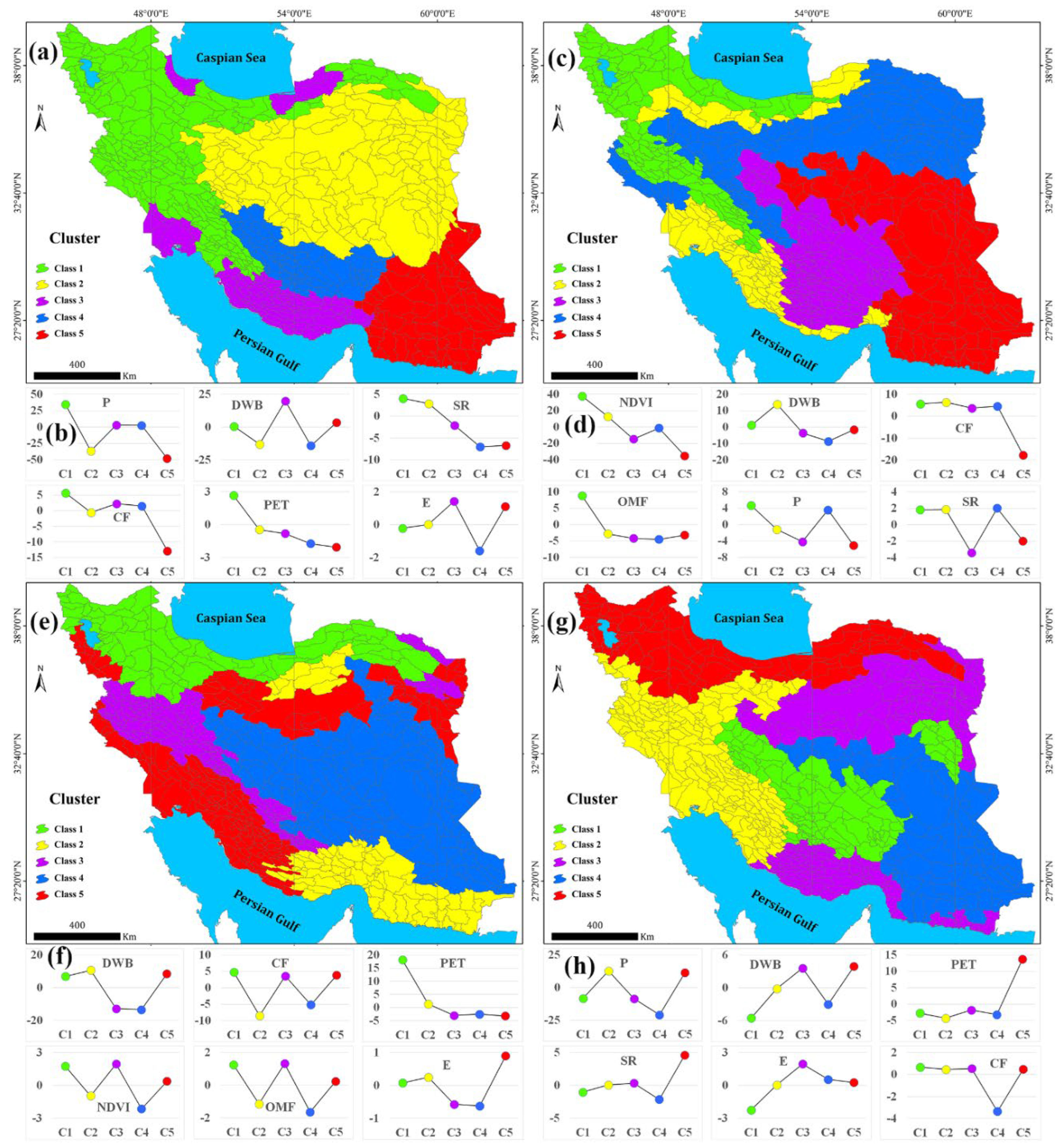
The SHAP model yielded a large number of coefficients for the 609 studied catchments, presenting a challenge in terms of interpretation. Hence, there is a requirement for a methodology to categorize the non-stationarity results of factors influencing SSM across seasons in Iran. In this study, cluster analysis was used to process SHAP coefficients. Following the clustering process, there is a discernible resemblance in the factors affecting catchments grouped within the same category. When comparing these categories, the results inherently manifest substantial distinctions in the various factors across catchments. In SPSS software, the two-step clustering algorithm automatically assesses the suitability of segmenting catchments into multiple categories by considering lower BIC values. Once it automatically determines the optimal number of clusters, it becomes possible to gain more precise insights into the distinctions among these categories. The results of clustering enable us to comprehend the extent to which each factor influences SSM in every cluster. In this study, catchments were automatically classified into five types, as the clustering yielded the lowest BIC index at this point. Table 3 presents the average SHAP values of the six primary factors for every season and class. Figure 7 displays the spatial distribution of the clustering results for various catchments. Coefficients with significant absolute values carry a more pronounced influence on the SSM. These figures serve as valuable tools for comprehending each catchment type's spatial arrangement and identifying the factors that exert the most substantial influence on each catchment's SSM.
The clustering results for winter are shown in Figure 7a,e. The first catchment types are located mainly in northwestern and western Iran. In these catchments, the factors that most significantly affect SSM are, in respective order, precipitation, clay fraction, solar radiation, potential evapotranspiration, distance from water bodies, and elevation, as illustrated in Figure 7a,e and detailed in Table 3. Akbari Majdar et al. (2018) investigated the spatial and temporal variations in SSM with respect to topographic and meteorological factors in Ardabil province, which falls into the first catchments category of this study. Their research underscored a significant correlation between SSM and variables such as precipitation. The second type of catchments is primarily found in central, eastern, and northeastern Iran. The most influential factors affecting SSM in these catchments are precipitation, distance from water bodies, solar radiation, clay fraction, potential evapotranspiration, and elevation. The third catchment category is predominantly located in southern and northern Iran, in proximity to the Persian Gulf and Caspian Sea. Within this catchment type, the most pivotal factor affecting SSM is the distance from water bodies, with precipitation, clay fraction, solar radiation, elevation, and potential evapotranspiration following in significance. In the fourth catchment category, similar to the third catchment type, the primary factor influencing SSM is the distance from water bodies, albeit with an inverse effect. This is followed by solar radiation, precipitation, potential evapotranspiration, elevation, and clay fraction (Table 3). The fifth catchment category is distributed in southeastern Iran. In order of influence, the most significant factors on SSM are precipitation, clay fraction, solar radiation, distance from water bodies, potential evapotranspiration, and elevation.
The clustering results for the spring season are shown in Figure 7b,f. In this season, vegetation and organic matter fraction have a higher impact on SSM than in winter. The first catchment type is located mainly in north, northwestern and western Iran. Within these catchments, the factors exerting the most substantial influence on SSM are, in their respective order of impact: NDVI, organic matter fraction, clay fraction, precipitation, solar radiation, and distance from water bodies, as demonstrated in Figure 7 and expounded upon in Table 3. The second catchment type is mainly distributed in southern, southwestern, and north Iran. Factors that most significantly affect SSM are distance from water bodies, NDVI, clay fraction, organic matter fraction, solar radiation, and precipitation. In the spring of 2020, Bandak et al. (2023) collected 394 surface soil samples in the Gorgan province located northern Iran, a region which is located in the second catchment type of this study. The findings of their research demonstrated a strong correlation between NDVI and SSM. The third catchment category is primarily located in southern and central Iran. Within this catchment category, the most dominant factor affecting SSM is the NDVI, with organic matter fraction, precipitation, clay fraction, distance from water bodies, and solar radiation subsequently ranking in significance. In the fourth catchment category, the predominant factor influencing SSM is the distance from water bodies. This is followed by clay fraction, organic matter fraction, precipitation, solar radiation, and NDVI (Table 3). The fifth catchment category is distributed in southeastern and eastern Iran. The most significant factors on SSM are NDVI, clay fraction, precipitation, organic matter fraction, solar radiation, and distance from water bodies.
Figure. 7c.g and Table 3 indicate the clustering results for the summer season. During this season, the influence of distance from water bodies and clay fraction on SSM is more pronounced compared to other seasons. The first catchment type is located in northern, northwestern and northeastern Iran around the Caspian Sea. In these catchments, the most significant influences on SSM are associated with potential evapotranspiration, proximity to water bodies, clay fraction, NDVI, organic matter fraction, and elevation (Fig 7c,g and Table 3). The second catchment type is mainly located in southern and southeastern Iran around the Persian Gulf and the Gulf of Oman. In this class, distance from water bodies is the most important factor, followed by clay fraction, potential evapotranspiration, organic matter fraction, NDVI, and elevation. In the third and fourth catchment categories, the hierarchy of factors' influence closely mirrors that of the second catchment type, except for the notable difference that NDVI exerts a more significant influence than the organic matter fraction. The fifth catchment category is primarily located in southeastern and eastern Iran. The most influential factors are distance from water bodies, clay fraction, potential evapotranspiration, elevation, NDVI, and organic matter fraction (Table 3).
The clustering results for autumn are shown in Figure 7d,h and Table 3. As precipitation begins in Iran, it becomes the predominant factor affecting SSM in most classes. The first catchment category is primarily located in central and eastern Iran. Within these catchments, the factors exerting the most substantial influence on SSM are precipitation, distance from water bodies, potential evapotranspiration, elevation, solar radiation, and clay fraction, as demonstrated in Figure 7d,h and described in Table 3. The second catchment type is mainly distributed in southwestern and western Iran. The factors that most significantly affect SSM are precipitation, potential evapotranspiration, clay fraction, distance from water bodies, solar radiation, and elevation. The third catchment category is primarily located in southern (near the Persian Gulf) and northeastern Iran. In this catchment type, precipitation is the most influential factor on SSM, followed by the distance from water bodies, elevation, potential evapotranspiration, clay fraction, and solar radiation. In the fourth catchment category, the primary influencing factors on SSM are precipitation and clay fraction, potential evapotranspiration, distance from water bodies, solar radiation, and elevation (Table 3). Finally, the fifth catchment category is distributed in northern Iran near the Caspian Sea. The most significant factors on SSM are potential evapotranspiration, precipitation, distance from water bodies, solar radiation, clay fraction, and elevation.
4. Conclusion
In this study, we unravelled the impact of the spatial non-stationarity of the critical environmental factors influencing SSM. To this end, we have introduced a framework that combines the SHAP technique with a two-step clustering analysis to provide spatial interpretations for machine learning models such as RF. Considering poor in-situ data of SSM in Iran, we initially validated the global SSM datasets, which include SMAP, MERRA-2, and CFSv2 at a depth of 0-5 cm, against in-situ data. The main conclusions are as follows:
1) Results of dataset validation of SSM demonstrated that among the datasets, SMAP exhibited the highest median correlation and the lowest median root mean square error when compared to in-situ stations. Hence, it is recommended for applications such as hydrological modelling, water resources management, and drought monitoring in Iran, where SSM data is scarce.
2) Investigation of SSM in the different land cover in Iran revealed significant variations in SSM across land cover. So that, forests and bare/sparse vegetation regions exhibited the highest and lowest SSM with a median value of 0.180 m3/m3 and 0.093 m3/m3, respectively. These findings highlight the importance of understanding the spatial distribution of SSM in different land cover types, which can have implications for various environmental and ecological processes.
3) Findings indicated that the RF model can offer SSM estimates with R2 values of 0.89, 0.83, 0.70, and 0.75 for the winter, spring, summer, and autumn seasons, respectively. This finding highlights the importance of seasonal investigation of SSM. With a shortage of SSM in the dry season, machine learning methods can't model SSM with very high accuracy.
4) The findings of the SHAP model and two-step cluster analysis indicated that winter and autumn SSM is primarily influenced by climatic factors. In contrast, spring and summer SSM is predominantly affected by vegetation and soil characteristics. These findings highlight the dynamic nature of SSM and how it is influenced by different environmental factors that change with the seasons. Understanding these seasonal variations is essential for effective SSM management and prediction in various regions.
Supplementary Materials
The following supporting information can be downloaded at the website of this paper posted on Preprints.org.
Declaration of competing interest: The authors declare that they have no known competing financial interests or personal relationships that could have appeared to influence the work reported in this paper.
Acknowledgments
The authors thank the Iran Meteorological Organization, which provided SSM and precipitation data for this paper.
References
- Adab, H., Morbidelli, R., Saltalippi, C., Moradian, M., Ghalhari, G.A.F., 2020. Machine learning to estimate surface soil moisture from remote sensing data. Water. 12, 3223. [CrossRef]
- Ahmad, S., Kalra, A., Stephen, H., 2010. Estimating soil moisture using remote sensing data: A machine learning approach. Adv. Water Resour. 33, 69-80. [CrossRef]
- Ali, I., Greifeneder, F., Stamenkovic, J., Neumann, M., Notarnicola, C., 2015. Review of machine learning approaches for biomass and soil moisture retrievals from remote sensing data. Remote Sens. 7, 16398-16421. [CrossRef]
- Amani, M., Ghorbanian, A., Ahmadi, S. A., Kakooei, M., Moghimi, A., Mirmazloumi, S. M., & Brisco, B., 2020. Google earth engine cloud computing platform for remote sensing big data applications: A comprehensive review. IEEE J. Sel. Top. Appl. Earth Obs. Remote Sens. 13, 5326-5350. [CrossRef]
- Amini, A., Moghadam, M. K., Kolahchi, A. A., Raheli-Namin, M., & Ahmed, K. O., 2023. Evaluation of GLDAS soil moisture product over Kermanshah province, Iran. H2Open J. 6(3), 373-386. [CrossRef]
- Amini, S., Saber, M., Rabiei-Dastjerdi, H., & Homayouni, S., 2022. Urban land use and land cover change analysis using random forest classification of landsat time series. Remote Sens. 14(11), 2654. [CrossRef]
- Ashraf, S., Nazemi, A., & AghaKouchak, A., 2021. Anthropogenic drought dominates groundwater depletion in Iran. Sci. Rep. 11(1), 9135. [CrossRef]
- Bandak, S., Movahedi Naeini, S. A. R., Komaki, C. B., Verrelst, J., Kakooei, M., & Mahmoodi, M. A., 2023. Satellite-Based Estimation of Soil Moisture Content in Croplands: A Case Study in Golestan Province, North of Iran. Remote Sens. 15(8), 2155. [CrossRef]
- Boueshagh, M., Hasanlou, M., 2019. Estimating water level in the Urmia Lake using satellite data: a machine learning approach. Int. arch. Photogramm. Remote Sens. Spatial Inf. Sci. 42, 219-226. [CrossRef]
- Boueshagh, M., Ramage, J.M., Brodzik, M.J., Long, D.G., Hardman, M. and Marshall, H.P., 2025. Revealing causes of a surprising correlation: snow water equivalent and spatial statistics from Calibrated Enhanced-Resolution Brightness Temperatures (CETB) using interpretable machine learning and SHAP analysis. Frontiers in Remote Sensing, 6, p.1554084. [CrossRef]
- Breiman, L., & Cutler, A., 2012. State of the art of data mining using Random forest. In Proc. Salford Data Mining Conf. San Diego, USA (pp. 24-25).
- Buitinck, L., Louppe, G., Blondel, M., Pedregosa, F., Mueller, A., Grisel, O., & Varoquaux, G., 2013. API design for machine learning software: experiences from the scikit-learn project. arXiv preprint arXiv:1309.0238. [CrossRef]
- Cai, Y., Zheng, W., Zhang, X., Zhangzhong, L., Xue, X., 2019. Research on soil moisture prediction model based on deep learning. PloS One. 14, e0214508. [CrossRef]
- Carranza, C., Nolet, C., Pezij, M., van der Ploeg, M., 2021. Root zone soil moisture estimation with Random Forest. J. Hydrol. 593, 125840. [CrossRef]
- Chen, F., Crow, W. T., Bindlish, R., Colliander, A., Burgin, M. S., Asanuma, J., & Aida, K., 2018. Global-scale evaluation of SMAP, SMOS and ASCAT soil moisture products using triple collocation. Remote Sens. Environ. 214, 1-13. [CrossRef]
- Chen, X., Hu, Q., 2004. Groundwater influences on soil moisture and surface evaporation. J. Hydrol. 297, 285-300. [CrossRef]
- Chiu, T., Fang, D., Chen, J., Wang, Y., & Jeris, C., 2001. A robust and scalable clustering algorithm for mixed type attributes in large database environment. In Proc. 7th ACM SIGKDD Int. Conf. on Knowledge Discovery and Data Mining (pp. 263–268). [CrossRef]
- Cho, E., & Choi, M., 2014. Regional scale spatio-temporal variability of soil moisture and its relationship with meteorological factors over the Korean peninsula. J. Hydrol. 516, 317-329. [CrossRef]
- Choubin, B., Darabi, H., Rahmati, O., Sajedi-Hosseini, F., & Kløve, B., 2018. River suspended sediment modelling using the CART model: A comparative study of machine learning techniques. Sci. Total Environ. 615, 272-281. [CrossRef]
- Colliander, A., Cosh, M. H., Misra, S., Jackson, T. J., Crow, W. T., Chan, S., & Yueh, S. H., 2017. Validation and scaling of soil moisture in a semiarid environment: SMAP validation experiment 2015 (SMAPVEX15). Remote Sens. Environ. 196, 101-112. [CrossRef]
- Copernicus (2023) Sentinel-2 data.
- Cosby, B., Hornberger, G., Clapp, R., Ginn, T., 1984. A statistical exploration of the relationships of soil moisture characteristics to the physical properties of soils. Water Resour. Res. 20, 682-690. [CrossRef]
- Cosh, M.H., Jackson, T.J., Moran, S., Bindlish, R., 2008. Temporal persistence and stability of surface soil moisture in a semiarid watershed. Remote Sens. Environ. 112, 304-313. [CrossRef]
- de Oliveira, V. A., Rodrigues, A. F., Morais, M. A. V., Terra, M. D. C. N. S., Guo, L., & de Mello, C. R., 2021. Spatiotemporal modelling of soil moisture in an A tlantic forest through machine learning algorithms. Eur. J. Soil Sci. 72(5), 1969-1987. [CrossRef]
- de Queiroz, M.G., da Silva, T.G.F., Zolnier, S., Jardim, A.M.d.R.F., de Souza, C.A.A., Júnior, G.d.N.A., de Morais, J.E.F., de Souza, L.S.B., 2020. Spatial and temporal dynamics of soil moisture for surfaces with a change in land use in the semiarid region of Brazil. Catena. 188, 104457. [CrossRef]
- Dirmeyer, P. A., & Halder, S., 2016. Sensitivity of numerical weather forecasts to initial soil moisture variations in CFSv2. Weather Forecasting. 31(6), 1973-1983. [CrossRef]
- D'Odorico, P., Caylor, K., Okin, G.S., Scanlon, T.M., 2007. On soil moisture–vegetation feedbacks and their possible effects on the dynamics of dryland ecosystems. J. Geophys. Res.: Biogeosci. 112. [CrossRef]
- Dorigo, W., Himmelbauer, I., Aberer, D., Schremmer, L., Petrakovic, I., Zappa, L., Preimesberger, W., Xaver, A., Annor, F., Ardö, J., 2021. The International Soil Moisture Network: serving Earth system science for over a decade. Hydrol. Earth Syst. Sci. 25, 5749-5804. DOI: 10.5194/hess-25-5749-2021.
- Du Toit, W., 2008. Radial basis function interpolation (Doctoral dissertation, Stellenbosch: Stellenbosch University).
- Du, M., Zhang, J., Elmahdi, A., Wang, Z., Yang, Q., Liu, H., & Wang, G., 2021. Variation characteristics and influencing factors of soil moisture content in the lime concretion black soil region in Northern Anhui. Water. 13(16), 2251. [CrossRef]
- Ekmekcioğlu, Ö., Koc, K., Özger, M., & Işık, Z., 2022. Exploring the additional value of class imbalance distributions on interpretable flash flood susceptibility prediction in the Black Warrior River basin, Alabama, United States. J. Hydrol., 610, 127877. [CrossRef]
- English, N. B., Weltzin, J. F., Fravolini, A., Thomas, L., & Williams, D. G., 2005. The influence of soil texture and vegetation on soil moisture under rainout shelters in a semi-desert grassland. J. Arid. Environ. 63(1), 324-343. [CrossRef]
- ESA-WorldCover., 2020. Worldwide Land Cover Mapping: VITO NV.2021. https://es a-worldcover.org/en.
- ESRI, A. N. A. & Guide, D. D. Spatial analysis, 14-15 (California, 2013).
- Everson, C., Mengistu, M., Vather, T., 2017. The validation of the variables (evaporation and soil water) in hydrometeorological models: Phase II, Application of cosmic ray probes for soil water measurement. Water Res. Comm. Pretoria S. Afr. WRC Rep 17.
- Fahrudin, T., Wijaya, D. R., & Agung, A. A. G., 2020. Covid-19 confirmed case correlation analysis based on spearman and kendall correlation. In 2020 Int. Conf. on Data Science and Its Appl. (ICoDSA) (pp. 1-4). IEEE. [CrossRef]
- Fahy, B., Brenneman, E., Chang, H., & Shandas, V., 2019. Spatial analysis of urban flooding and extreme heat hazard potential in Portland, OR. Int. J. Disaster Risk Reduct. 39, 101117. [CrossRef]
- Fakharizadehshirazi, E., Sabziparvar, A. A., & Sodoudi, S., 2019. Long-term spatiotemporal variations in satellite-based soil moisture and vegetation indices over Iran. Environ. Earth Sci. 78, 1-14. [CrossRef]
- Fan, Y., Li, H., & Miguez-Macho, G., 2013. Global patterns of groundwater table depth. Science. 339(6122), 940-943. [CrossRef]
- Fathololoumi, S., Vaezi, A. R., Alavipanah, S. K., Ghorbani, A., & Biswas, A., 2020. Comparison of spectral and spatial-based approaches for mapping the local variation of soil moisture in a semiarid mountainous area. Sci. Total Environ. 724, 138319. [CrossRef]
- Feng, H., & Liu, Y., 2015. Combined effects of precipitation and air temperature on soil moisture in different land covers in a humid basin. J. Hydrol. 531, 1129-1140. [CrossRef]
- Fu, X., Jiang, X., Yu, Z., Ding, Y., Lü, H., & Zheng, D., 2022. Understanding the key factors that influence soil moisture estimation using the unscented weighted ensemble Kalman filter. Agric. For. Meteorol. 313, 108745. [CrossRef]
- Garcia-Estringana, P., Latron, J., Llorens, P., & Gallart, F., 2013. Spatial and temporal dynamics of soil moisture in a Mediterranean mountain area (Vallcebre, NE Spain). Ecohydrology, 6(5), 741-753. [CrossRef]
- Gelaro, R., McCarty, W., Su´arez, M.J., et al., 2017. The modern-era retrospective analysis for research and applications, version 2 (MERRA-2). J. Clim. 30, 5419–5454. [CrossRef]
- Ghasemloo, N., Matkan, A. A., Alimohammadi, A., Aghighi, H., & Mirbagheri, B., 2022. Estimating the agricultural farm soil moisture using spectral indices of Landsat 8, and Sentinel-1, and artificial neural networks. J. Geovisualization Spatial Anal. 6(2), 19. [CrossRef]
- Gheybi, F., Paridad, P., Faridani, F., Farid, A., Pizarro, A., Fiorentino, M., & Manfreda, S., 2019. Soil moisture monitoring in Iran by implementing satellite data into the root-zone SMAR model. Hydrology. 6(2), 44. [CrossRef]
- Gökhan, A. K. S. U., Güzeller, C. O., & Eser, M. T., 2019. The effect of the normalization method used in different sample sizes on the success of artificial neural network model. Int. j. assess. tool. educ. 6(2), 170-192. [CrossRef]
- Goward, S. N., Markham, B., Dye, D. G., Dulaney, W., & Yang, J., 1991. Normalized difference vegetation index measurements from the Advanced Very High Resolution Radiometer. Remote Sens. Environ. 35(2-3), 257-277. [CrossRef]
- Grayson, R.B., Western, A.W., Chiew, F.H., Blöschl, G., 1997. Preferred states in spatial soil moisture patterns: Local and nonlocal controls. Water Resour. Res. 33, 2897-2908. [CrossRef]
- Gruber, A., Dorigo, W.A., Zwieback, S., Xaver, A., Wagner, W., 2013. Characterizing coarse-scale representativeness of in situ soil moisture measurements from the International Soil Moisture Network. Vadose Zone J. 12. [CrossRef]
- Guevara, M., Taufer, M., Vargas, R., 2021. Gap-free global annual soil moisture: 15 km grids for 1991–2018. Earth Syst. Sci. Data, 13, 1711-1735. DOI: 10.5194/essd-13-1711-2021.
- Gupta, H. V., Kling, H., Yilmaz, K. K., & Martinez, G. F., 2009. Decomposition of the mean squared error and NSE performance criteria: Implications for improving hydrological modelling. J. Hydrol. 377(1-2), 80-91. [CrossRef]
- Han, Q., Zeng, Y., Zhang, L., Wang, C., Prikaziuk, E., Niu, Z., & Su, B., 2023. Global long term daily 1 km surface soil moisture dataset with physics informed machine learning. Sci. Data. 10(1), 101. [CrossRef]
- He, Z., Zhao, W., Liu, H., & Chang, X., 2012. The response of soil moisture to rainfall event size in subalpine grassland and meadows in a semiarid mountain range: A case study in northwestern China’s Qilian Mountains. J. Hydrol., 420, 183-190. [CrossRef]
- Hengl, T., Mendes de Jesus, J., Heuvelink, G. B., Ruiperez Gonzalez, M., Kilibarda, M., Blagotić, A., & Kempen, B., 2017. SoilGrids250m: Global gridded soil information based on machine learning. PLoS One. 12(2), e0169748. [CrossRef]
- IMO., 2019. Iran Meteorological Organization. https://www.irimo.ir.
- IMO., 2023. Iran Meteorological Organization. https://www.irimo.ir.
- IWRMC., 2023. Iran Water Resources Management Company. https://www.wrm.ir.
- Jamei, M., Lopez-Baeza, E., & Asadi, E., 2022. Validation of SMAP Surface Soil Moisture Products over Iran. 44th COSPAR Sci. Assem., Held 16-24 July, 44, 123.
- Jamei, M., Mousavi Baygi, M., Oskouei, E. A., & Lopez-Baeza, E. (2020). Validation of the SMOS level 1C brightness temperature and level 2 soil moisture data over the west and southwest of Iran. Remote Sens. 12(17), 2819. [CrossRef]
- Javari, M., 2016. Trend and homogeneity analysis of precipitation in Iran. Climate. 4(3), 44. [CrossRef]
- Jawson, S. D., & Niemann, J. D., 2007. Spatial patterns from EOF analysis of soil moisture at a large scale and their dependence on soil, land-use, and topographic properties. Adv. Water Resour. 30(3), 366-381. [CrossRef]
- Jiang, Z., Huete, A. R., Didan, K., & Miura, T., 2008. Development of a two-band enhanced vegetation index without a blue band. Remote Sens. Environ. 112(10), 3833-3845. [CrossRef]
- Jin, Z., Guo, L., Lin, H., Wang, Y., Yu, Y., Chu, G., & Zhang, J., 2018. Soil moisture response to rainfall on the Chinese Loess Plateau after a long-term vegetation rehabilitation. Hydrol. Processes. 32(12), 1738-1754. [CrossRef]
- Jung, M., Reichstein, M., Ciais, P., Seneviratne, S.I., Sheffield, J., Goulden, M.L., Bonan, G., Cescatti, A., Chen, J., De Jeu, R., 2010. Recent decline in the global land evapotranspiration trend due to limited moisture supply. Nature. 467, 951-954. [CrossRef]
- Kaiser, M., Günnemann, S., & Disse, M., 2022. Regional-scale prediction of pluvial and flash flood susceptible areas using tree-based classifiers. J. Hydrol. 612, 128088. [CrossRef]
- Khosravi, K., Panahi, M., Golkarian, A., Keesstra, S. D., Saco, P. M., Bui, D. T., & Lee, S., 2020. Convolutional neural network approach for spatial prediction of flood hazard at national scale of Iran. J. Hydrol. 591, 125552. [CrossRef]
- Kimball, J.S., Jones, L.A., Endsley, A., et al., 2018. SMAP L4 Global Daily 9 Km EASE-Grid Carbon Net Ecosystem Exchange, Version 4. In: In NASA (Ed.). Boulder, Colorado USA. [CrossRef]
- Kling, H., Fuchs, M., & Paulin, M., 2012. Runoff conditions in the upper Danube basin under an ensemble of climate change scenarios. J. Hydrol., 424, 264-277. [CrossRef]
- Lagos, M., Serna, J. L., Muñoz, J. F., & Suárez, F., 2020. Challenges in determining soil moisture and evaporation fluxes using distributed temperature sensing methods. J. Environ. Manage. 261, 110232. [CrossRef]
- Laity, J. J., 2009. Deserts and desert environments (Vol. 3). John Wiley & Sons.
- Liu, Q., Gui, D., Zhang, L., Niu, J., Dai, H., Wei, G., & Hu, B. X., 2022. Simulation of regional groundwater levels in arid regions using interpretable machine learning models. Sci. Total Environ. 831, 154902. [CrossRef]
- Lundberg, S. M., & Lee, S. I., 2017. A unified approach to interpreting model predictions. Adv. Neural Inf. Process. Syst. 30. [CrossRef]
- Majdar, H. A., Vafakhah, M., Sharifikia, M., & Ghorbani, A., 2018. Spatial and temporal variability of soil moisture in relation with topographic and meteorological factors in south of Ardabil Province, Iran. Environ. Monit. Assess. 190, 1-12. [CrossRef]
- Maleki, K. H., Vaezi, A. R., & Sarmadian, F., 2019. Validation of satellite-based soil moisture retrievals from SMAP with in situ observation in the Simineh-Zarrineh (Bokan) Catchment, NW of Iran. Eurasian J. Soil Sci. 8(4), 340-350. [CrossRef]
- Meng, F., Luo, M., Sa, C., Wang, M., & Bao, Y., 2022. Quantitative assessment of the effects of climate, vegetation, soil and groundwater on soil moisture spatiotemporal variability in the Mongolian Plateau. Sci. Total Environ. 809, 152198. [CrossRef]
- Muñoz-Sabater, J., Dutra, E., Agustí-Panareda, A., Albergel, C., Arduini, G., Balsamo, G., Boussetta, S., Choulga, M., Harrigan, S., Hersbach, H., 2021. ERA5-Land: A state-of-the-art global reanalysis dataset for land applications. Earth Syst. Sci. Data. 13, 4349–4383. DOI: 10.5194/essd-13-4349-2021.
- Naghibi, S. A., Pourghasemi, H. R., & Dixon, B., 2016. GIS-based groundwater potential mapping using boosted regression tree, classification and regression tree, and random forest machine learning models in Iran. Environ. Monit. Assess. 188, 1-27. [CrossRef]
- Nikraftar, Z., Mostafaie, A., Sadegh, M., Afkueieh, J. H., & Pradhan, B., 2021a. Multi-type assessment of global droughts and teleconnections. Weather Clim. Extremes. 34, 100402. [CrossRef]
- Nikraftar, Z., Parizi, E., Hosseini, S. M., & Ataie-Ashtiani, B., 2021b. Lake Urmia restoration success story: A natural trend or a planned remedy? J. Great Lakes Res. 47(4), 955-969. [CrossRef]
- Nikraftar, Z., Parizi, E., Saber, M., Hosseini, S. M., Ataie-Ashtiani, B., & Simmons, C. T. (2023). Groundwater sustainability assessment in the Middle East using GRACE/GRACE-FO data. Hydrogeol. J. 1-17. [CrossRef]
- NOAA, National Oceanic and Atmospheric Administration., 2023. Climate Change. NOAA. https://www.noaa.gov/climate-change. https://www.noaa.gov/.
- Ojha, R., Morbidelli, R., Saltalippi, C., Flammini, A., & Govindaraju, R. S., 2014. Scaling of surface soil moisture over heterogeneous fields subjected to a single rainfall event. J. Hydrol. 516, 21-36. [CrossRef]
- Parizi, E., Bagheri-Gavkosh, M., Hosseini, S. M., & Geravand, F., 2021. Linkage of geographically weighted regression with spatial cluster analyses for regionalization of flood peak discharges drivers: Case studies across Iran. J. Cleaner Prod. 310, 127526. [CrossRef]
- Parizi, E., Hosseini, S. M., Ataie-Ashtiani, B., & Simmons, C. T., 2020. Normalized difference vegetation index as the dominant predicting factor of groundwater recharge in phreatic aquifers: case studies across Iran. Sci. Rep. 10(1), 17473. [CrossRef]
- Parizi, E., Hosseini, S. M., Ataie-Ashtiani, B., & Simmons, C. T., 2019. Representative pumping wells network to estimate groundwater withdrawal from aquifers: Lessons from a developing country, Iran. J. Hydrol. 578, 124090. [CrossRef]
- Parizi, E., Khojeh, S., Hosseini, S. M., & Moghadam, Y. J., 2022. Application of Unmanned Aerial Vehicle DEM in flood modeling and comparison with global DEMs: Case study of Atrak River Basin, Iran. J. Environ. Manage. 317, 115492. [CrossRef]
- Patel, N. R., Anapashsha, R., Kumar, S., Saha, S. K., & Dadhwal, V. K., 2009. Assessing potential of MODIS derived temperature/vegetation condition index (TVDI) to infer soil moisture status. Int. J. Remote Sens. 30(1), 23-39. [CrossRef]
- Pedregosa, F., Varoquaux, G., Gramfort, A., Michel, V., Thirion, B., Grisel, O., & Duchesnay, É., 2011. Scikit-learn: Machine learning in Python. J. Mach. Learn. Res. 12, 2825-2830.
- Pellet, C., & Hauck, C., 2017. Monitoring soil moisture from middle to high elevation in Switzerland: set-up and first results from the SOMOMOUNT network. Hydrol. Earth Syst. Sci. 21(6), 3199-3220. DOI: 10.5194/hess-21-3199-2017.
- Perry, M. A., & Niemann, J. D., 2007. Analysis and estimation of soil moisture at the catchment scale using EOFs. J. Hydrol. 334(3-4), 388-404. [CrossRef]
- Pouyan, S., Pourghasemi, H. R., Bordbar, M., Rahmanian, S., & Clague, J. J., 2021. A multi-hazard map-based flooding, gully erosion, forest fires, and earthquakes in Iran. Sci. Rep. 11(1), 14889. [CrossRef]
- Qin, H., Huang, Q., Zhang, Z., Lu, Y., Li, M., Xu, L., & Chen, Z., 2019. Carbon dioxide emission driving factors analysis and policy implications of Chinese cities: Combining geographically weighted regression with two-step cluster. Sci. Total Environ. 684, 413–424. [CrossRef]
- Raduła, M. W., Szymura, T. H., & Szymura, M., 2018. Topographic wetness index explains soil moisture better than bioindication with Ellenberg’s indicator values. Ecol. Indic. 85, 172-179. [CrossRef]
- Rahmani, A., Golian, S., & Brocca, L., 2016. Multiyear monitoring of soil moisture over Iran through satellite and reanalysis soil moisture products. Int. J. Appl. Earth Obs. Geoinf. 48, 85-95. [CrossRef]
- Rascón-Ramos, A. E., Martinez-Salvador, M., Sosa-Perez, G., Villarreal-Guerrero, F., Pinedo-Alvarez, A., Santellano-Estrada, E., & Corrales-Lerma, R., 2021. Soil moisture dynamics in response to precipitation and thinning in a semi-dry forest in Northern Mexico. Water. 13(1), 105. [CrossRef]
- Rasheed, M. W., Tang, J., Sarwar, A., Shah, S., Saddique, N., Khan, M. U., & Sultan, M., 2022. Soil moisture measuring techniques and factors affecting the moisture dynamics: A comprehensive review. Sustainability. 14(18), 11538. [CrossRef]
- Reichle, R. H., Draper, C. S., Liu, Q., Girotto, M., Mahanama, S. P., Koster, R. D., & De Lannoy, G. J., 2017. Assessment of MERRA-2 land surface hydrology estimates. J. Clim. 30(8), 2937-2960. [CrossRef]
- Reichle, R. H., Liu, Q., Koster, R. D., Crow, W. T., De Lannoy, G. J., Kimball, J. S., & Walker, J. P., 2019. Version 4 of the SMAP level-4 soil moisture algorithm and data product. J. Adv. Model. Earth Syst. 11(10), 3106-3130. [CrossRef]
- Running, S., Mu, Q., and Zhao, M., 2017. MOD16A2 MODIS/Terra Net Evapotranspiration 8-Day L4 Global 500m SIN Grid V006. NASA EOSDIS Land Processes DAAC. [CrossRef]
- Saadatabadi, A. R., Izadi, N., Karakani, E. G., Fattahi, E., & Shamsipour, A. A., 2021. Investigating relationship between soil moisture, hydro-climatic parameters, vegetation, and climate change impacts in a semiarid basin in Iran. Arabian J. Geosci. 14, 1-18. [CrossRef]
- Sadeghi, M., Shearer, E. J., Mosaffa, H., Gorooh, V. A., Naeini, M. R., Hayatbini, N., & Sorooshian, S., 2021. Application of remote sensing precipitation data and the CONNECT algorithm to investigate spatiotemporal variations of heavy precipitation: Case study of major floods across Iran (Spring 2019). J. Hydrol. 600, 126569. [CrossRef]
- Saeedi, M., Sharafati, A., & Tavakol, A., 2021. Evaluation of gridded soil moisture products over varied land covers, climates, and soil textures using in situ measurements: A case study of Lake Urmia Basin. Theor. Appl. Climatol., 145(3-4), 1053-1074. [CrossRef]
- Saemian, P., Hosseini-Moghari, S. M., Fatehi, I., Shoarinezhad, V., Modiri, E., Tourian, M. J., & Sneeuw, N., 2021. Comprehensive evaluation of precipitation datasets over Iran. J. Hydrol. 603, 127054. [CrossRef]
- Saha, S., & Tripp, P., 2011. CFSv2 retrospective forecasts. NOAA/NWS/NCEP Environmental Modeling Center Tech. Rep.
- Saha, S., Moorthi, S., Wu, X., Wang, J., Nadiga, S., Tripp, P., & Becker, E., 2014. The NCEP climate forecast system version 2. J. Clim. 27(6), 2185-2208. [CrossRef]
- Satish, S. M., & Bharadhwaj, S., 2010. Information search behaviour among new car buyers: A two-step cluster analysis. IIMB Manag. Rev. 22(1–2), 5–15. [CrossRef]
- Japan International Cooperation Agency, JICA (2016). Data Collection Survey on Improvement of Hydrological Cycle Model of Lake Urmia Basin. http://open_jicareport.jica.go.jp/pdf/12252292.pdf.
- Schwinning, S., Sala, O.E., 2004. Hierarchy of responses to resource pulses in arid and semiarid ecosystems. Oecologia 141, 211-220. [CrossRef]
- Seneviratne, S.I., Corti, T., Davin, E.L., Hirschi, M., Jaeger, E.B., Lehner, I., Orlowsky, B., Teuling, A.J., 2010. Investigating soil moisture–climate interactions in a changing climate: A review. Earth Sci. Rev. 99, 125-161. [CrossRef]
- Sivakumar, M. V., & Stefanski, R., 2007. Climate and land degradation—an overview (pp. 105-135). Springer Berlin Heidelberg. [CrossRef]
- Sure, A., & Dikshit, O., 2019. Estimation of root zone soil moisture using passive microwave remote sensing: A case study for rice and wheat crops for three states in the Indo-Gangetic basin. J. Environ. Manage. 234, 75-89. [CrossRef]
- Tabari, H., & Talaee, P. H., 2011. Temporal variability of precipitation over Iran: 1966–2005. J. Hydrol. 396(3-4), 313-320. [CrossRef]
- Tadono, T., Nagai, H., Ishida, H., Oda, F., Naito, S., Minakawa, K., & Iwamoto, H., 2016. Generation of the 30 m-mesh global digital surface model by ALOS PRISM. Int. arch. Photogramm. Remote Sens. Spatial Inf. Sci. 41, 157-162. DOI: 10.5194/isprs-archives-XLI-B4-157-2016.
- Tang, G., Clark, M. P., Papalexiou, S. M., Ma, Z., & Hong, Y., 2020. Have satellite precipitation products improved over last two decades? A comprehensive comparison of GPM IMERG with nine satellite and reanalysis datasets. Remote Sens. Environ. 240, 111697. [CrossRef]
- Tian, J., & Zhang, Y., 2023. Comprehensive validation of seven root zone soil moisture products at 1153 ground sites across China. Int. J. Digital Earth. 16(2), 4008-4022. [CrossRef]
- Tyralis, H., Papacharalampous, G., & Langousis, A., 2019. A brief review of random forests for water scientists and practitioners and their recent history in water resources. Water. 11(5), 910. [CrossRef]
- Vachaud, G., Passerat de Silans, A., Balabanis, P., & Vauclin, M., 1985. Temporal stability of spatially measured soil water probability density function. Soil Sci. Soc. Am. J. 49(4), 822-828. [CrossRef]
- Van den Broeck, G., Lykov, A., Schleich, M., & Suciu, D., 2022. On the tractability of SHAP explanations. J. Artif. Intell. Res. 74, 851-886. [CrossRef]
- Vanderlinden, K., Vereecken, H., Hardelauf, H., Herbst, M., Martínez, G., Cosh, M. H., & Pachepsky, Y. A., 2012. Temporal stability of soil water contents: A review of data and analyses. Vadose Zone J. 11(4). [CrossRef]
- Wang, S., Peng, H., & Liang, S., 2022. Prediction of estuarine water quality using interpretable machine learning approach. J. Hydrol. 605, 127320. [CrossRef]
- Wang, T., & Franz, T. E., 2015. Field observations of regional controls of soil hydraulic properties on soil moisture spatial variability in different climate zones. Vadose Zone J. 14(8). [CrossRef]
- Wang, Y., Yang, J., Chen, Y., Fang, G., Duan, W., Li, Y., & De Maeyer, P., 2019. Quantifying the effects of climate and vegetation on soil moisture in an arid area, China. Water. 11(4), 767. [CrossRef]
- Wenwu, Z. H. A. O., Xuening, F. A. N. G., Daryanto, S., Zhang, X., & Yaping, W. A. N. G., 2018. Factors influencing soil moisture in the Loess Plateau, China: A review. Earth Environ. Sci. Trans. R. Soc. Edinburgh, 109(3-4), 501-509. [CrossRef]
- Wu, X., Lu, G., Wu, Z., He, H., Scanlon, T., & Dorigo, W., 2020. Triple collocation-based assessment of satellite soil moisture products with in situ measurements in china: Understanding the error sources. Remote Sens. 12(14), 2275. [CrossRef]
- Xu, L., Chen, N., Zhang, X., Moradkhani, H., Zhang, C., & Hu, C., 2021a. In-situ and triple-collocation based evaluations of eight global root zone soil moisture products. Remote Sens. Environ. 254, 112248. [CrossRef]
- Xu, M., Xu, G., Cheng, Y., Min, Z., Li, P., Zhao, B., & Xiao, L., 2021b. Soil moisture estimation and its influencing factors based on temporal stability on a semiarid sloped forestland. Front. Earth Sci. 9, 629826. [CrossRef]
- Yang, Q., Fan, J., & Luo, Z., 2024. Response of soil moisture and vegetation growth to precipitation under different land uses in the Northern Loess Plateau, China. Catena, 236, 107728. [CrossRef]
- Zhang, L., Zeng, Y., Zhuang, R., Szabó, B., Manfreda, S., Han, Q., & Su, Z., 2021. In situ observation-constrained global surface soil moisture using random forest model. Remote Sens. 13(23), 4893. [CrossRef]
- Zhao, W., Sánchez, N., Lu, H., Li, A., 2018. A spatial downscaling approach for the SMAP passive surface soil moisture product using random forest regression. J. Hydrol. 563, 1009-1024. [CrossRef]
- Zhou, Q., Sun, Z., Liu, X., Wei, X., Peng, Z., Yue, C., & Luo, Y., 2019. Temporal soil moisture variations in different vegetation cover types in karst areas of southwest China: a plot scale case study. Water. 11(7), 1423. [CrossRef]
Figure 1.
The location of the study area and the agrometeorological stations with the climate classification and topography as the background.
Figure 1.
The location of the study area and the agrometeorological stations with the climate classification and topography as the background.
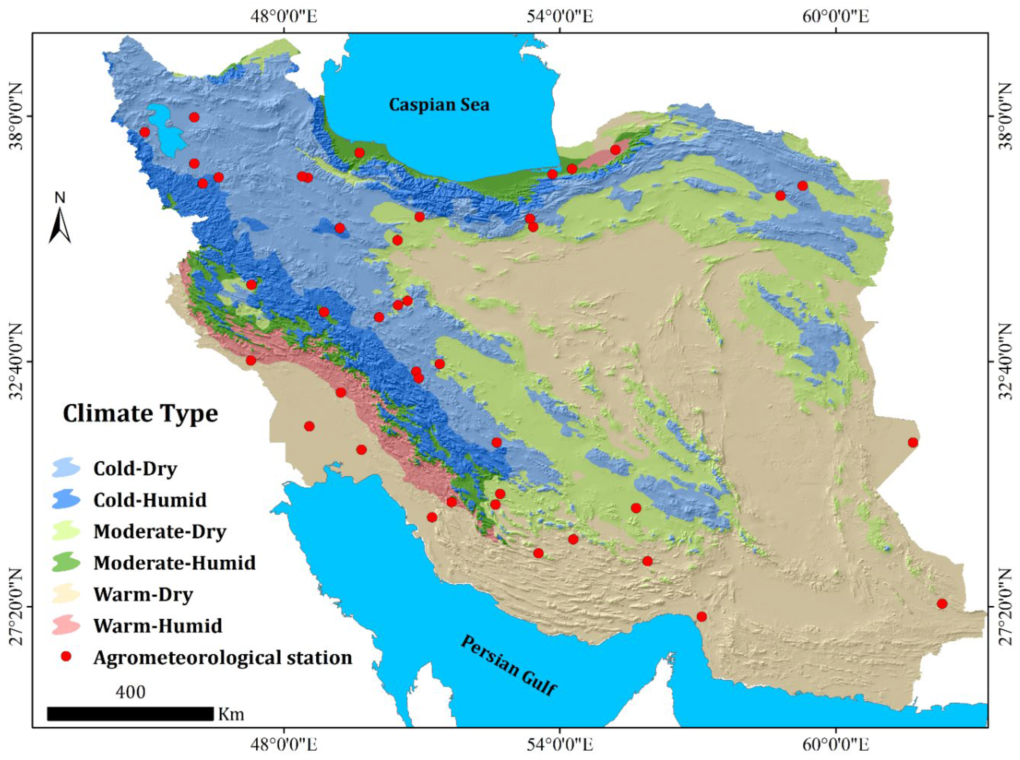
Figure 2.
The SSM evaluation based on in-situ data and statistical metrics of τ (a), KGE (b), RMSE (c), and RBias (d) from April 1, 2015, to March 31, 2023.
Figure 2.
The SSM evaluation based on in-situ data and statistical metrics of τ (a), KGE (b), RMSE (c), and RBias (d) from April 1, 2015, to March 31, 2023.
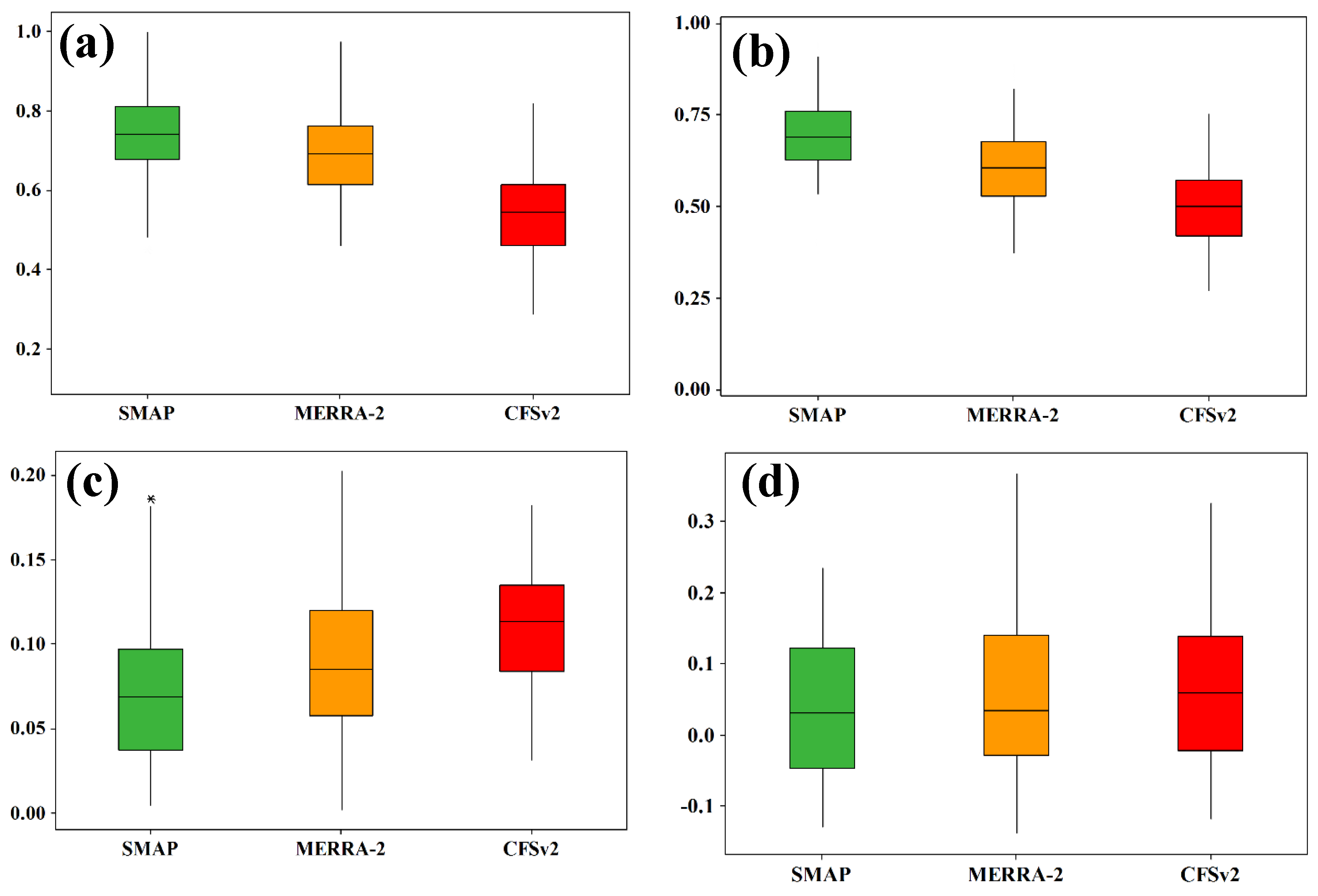
Figure 3.
Spatial pattern of SSM in winter (a), spring (b), summer (c), and autumn (d) in Iran’s 609 studied catchments from April 2015 to March 2023.
Figure 3.
Spatial pattern of SSM in winter (a), spring (b), summer (c), and autumn (d) in Iran’s 609 studied catchments from April 2015 to March 2023.
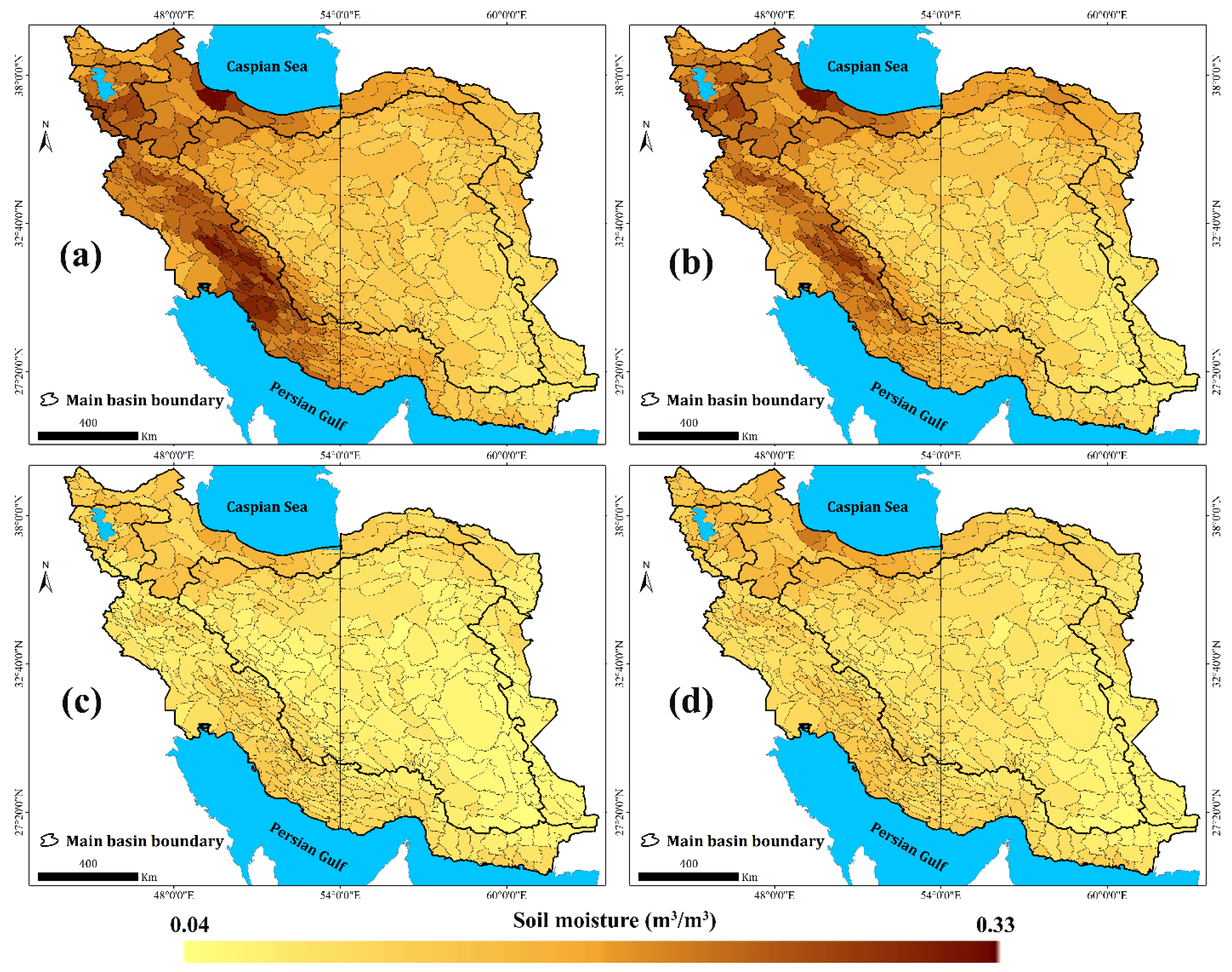
Figure 4.
Boxplot (a) and temporal pattern (b) of monthly SSM in various land covers across Iran from April 1, 2015, to March 31, 2023. The temporal pattern of precipitation is also illustrated in section b.
Figure 4.
Boxplot (a) and temporal pattern (b) of monthly SSM in various land covers across Iran from April 1, 2015, to March 31, 2023. The temporal pattern of precipitation is also illustrated in section b.
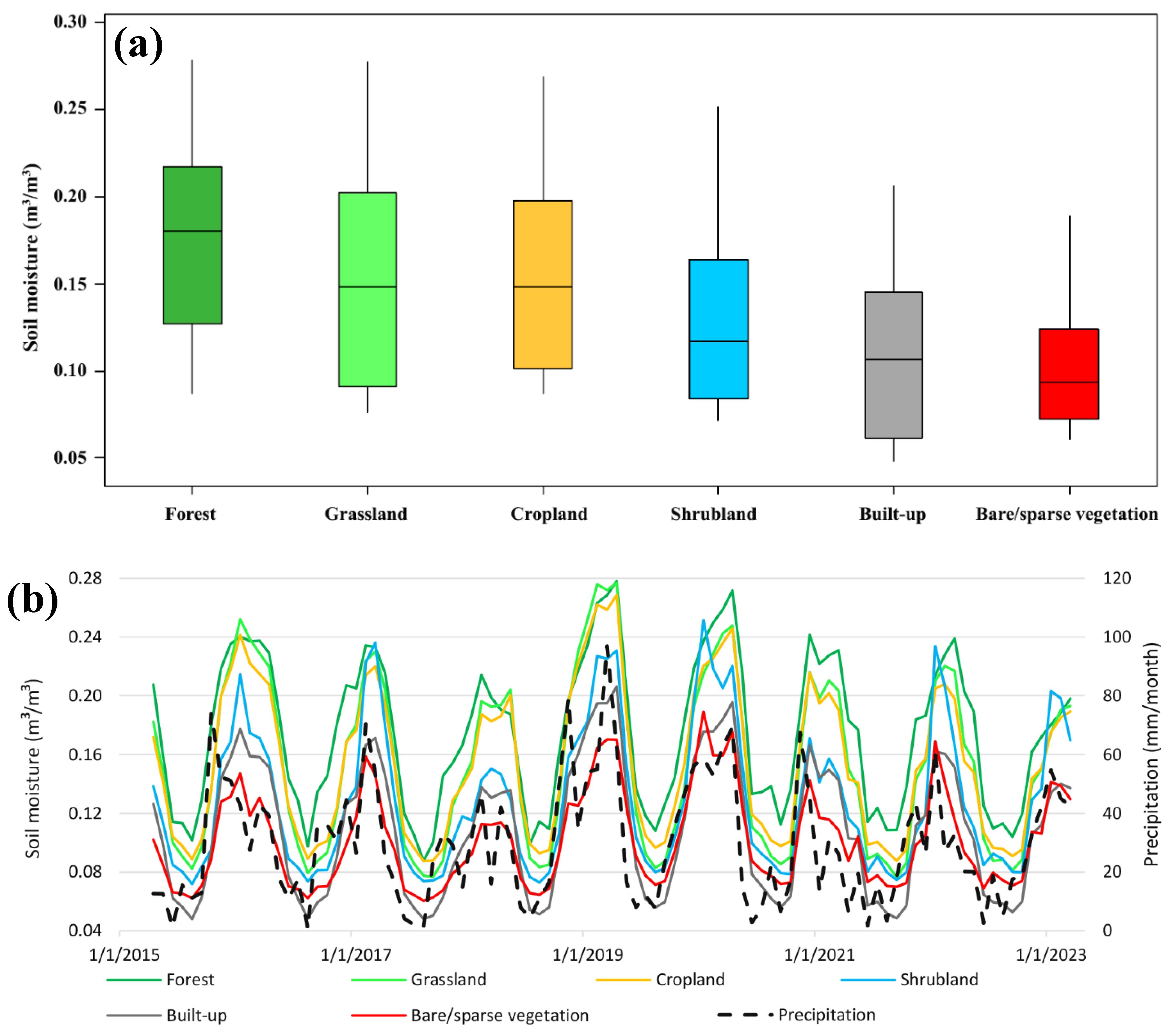
Figure 5.
The scatterplot, trend line, and R2 of the predicted and observed SSM in the testing phase: winter (a), spring (b), summer (c), and autumn (d).
Figure 5.
The scatterplot, trend line, and R2 of the predicted and observed SSM in the testing phase: winter (a), spring (b), summer (c), and autumn (d).
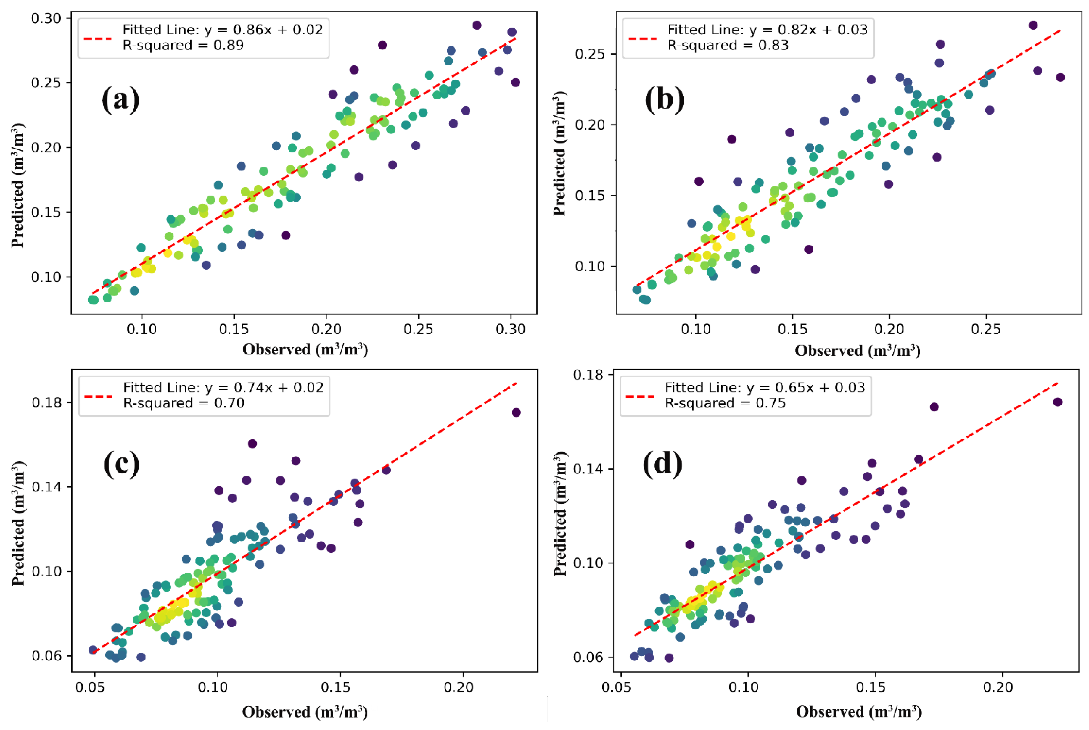
Figure 6.
SHAP plots reveal the effects of the influencing factors on the SSM: winter (a), spring (b), summer (c), and autumn (d). Each data point represents a SHAP value for a feature. P: precipitation, PET: potential evapotranspiration, SR: solar radiation, WS: wind speed, NDVI: normalized difference vegetation index, GWTD: groundwater table depth, DWB: distance from water bodies, CF: clay fraction, OMF: organic matter fraction, E: elevation, and TRI: topography roughness index.
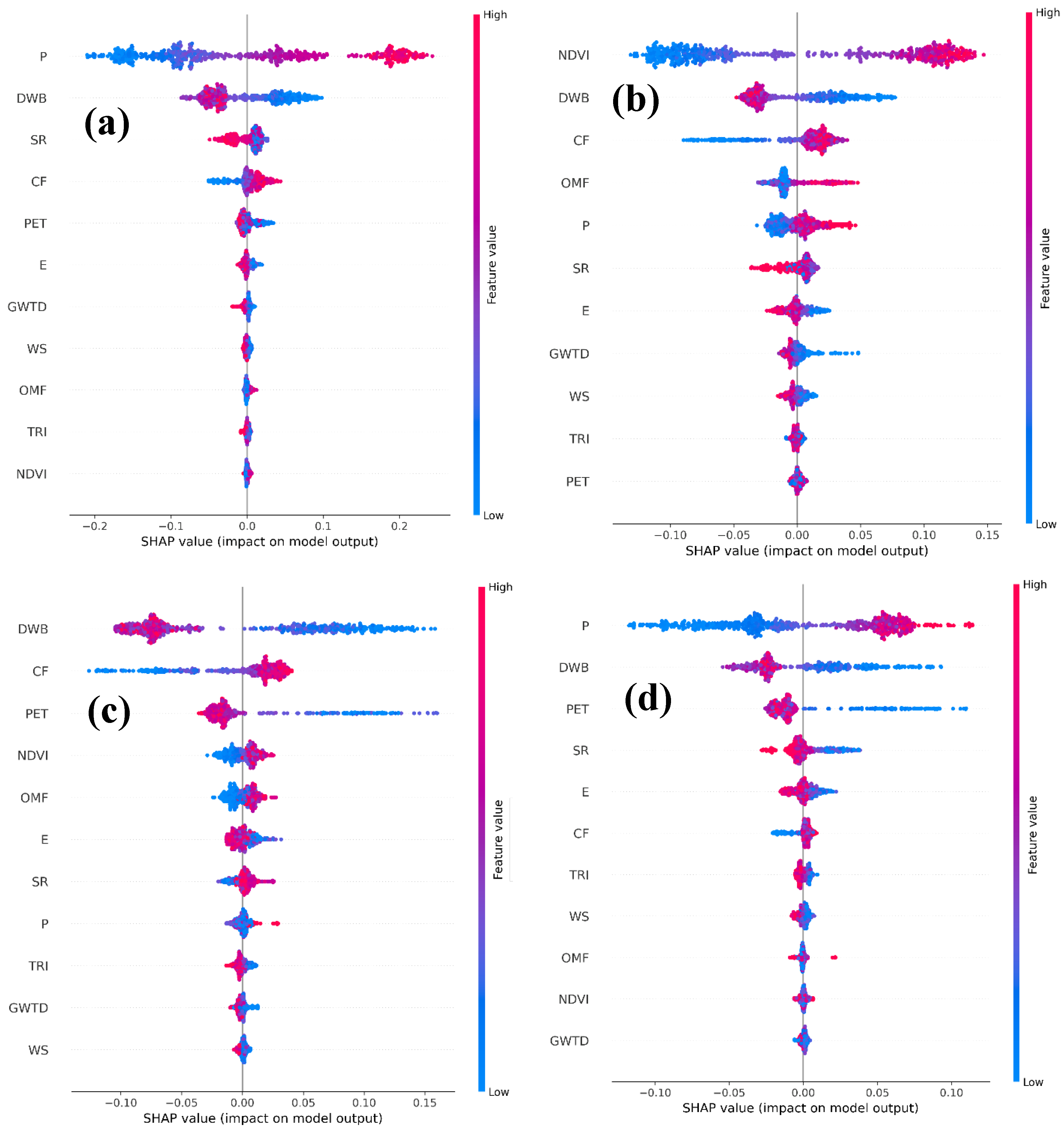
Figure 7.
Different types of catchments obtained by clustering the SHAP values for the winter (a and b), spring (c and d), summer (e and f), and autumn (g and h). P: precipitation, PET: potential evapotranspiration, SR: solar radiation, WS: wind speed, NDVI: normalized difference vegetation index, GWTD: groundwater table depth, DWB: distance from water bodies, CF: clay fraction, OMF: organic matter fraction, E: elevation, and TRI: topography roughness index. The SHAP values are multiplied by 1000 for visualization purposes.
Disclaimer/Publisher’s Note: The statements, opinions and data contained in all publications are solely those of the individual author(s) and contributor(s) and not of MDPI and/or the editor(s). MDPI and/or the editor(s) disclaim responsibility for any injury to people or property resulting from any ideas, methods, instructions or products referred to in the content. |
© 2025 by the authors. Licensee MDPI, Basel, Switzerland. This article is an open access article distributed under the terms and conditions of the Creative Commons Attribution (CC BY) license (http://creativecommons.org/licenses/by/4.0/).
Copyright: This open access article is published under a Creative Commons CC BY 4.0 license, which permit the free download, distribution, and reuse, provided that the author and preprint are cited in any reuse.


