Submitted:
13 May 2025
Posted:
14 May 2025
You are already at the latest version
Abstract
The Kerr-Newman solution to the Einstein field equations has a flat region spanning the ring singularity in the solution; which, unlike the Kerr solution, is not a disk. The nature of thisregion and its relation to the singularity are the subjects of this paper.
Keywords:
Kerr-Newman
; ring singularity
; flat regions
The metric for the charged Kerr solution, known as the Kerr–Newman solution, in Kerr-Schild coordinates is
where kμ is the null vector field
The variable r is given implicitly by
In Eq. (3), surfaces of constant r are confocal ellipsoids of revolution about the z-axis. Asymptotically, in Minkowski coordinates, r is the distance from the origin.
Define ρ := (x2 + y2)1/2. A ring singularity is located at ρ = a and z = 0. For the Kerr metric, this ring singularity bounds a surface having the character of a quadratic branch point in the complex plane; that is, if one passes through the surface from above (entering a region where, in Boyer-Lindquist coordinates, the coordinate labeling the oblate spheroidal surfaces of constant r is negative) and were to loop around the ring singularity to again pass through the surface from above, one would return to the original starting space. The Kerr solution in the negative r region is identical in structure to the positive r part with m being replaced by its negative. The geometry of Kerr-Newman solution in the region of the singularity is quite different.
The Kerr-Newman metric in the Kerr-Schild coordinates of Eq. (1) shows that the metric becomes flat when r = e2/2m. The flat region can then be found by solving Eq. (3), which determines r up to a sign, for r in terms of ρ. Perhaps the first person to make use of this flat region, albeit in the context of trying to find a classical model for the electron, was López.[1]
There are four solutions to Eq. (3) (two of which are imaginary), and the remaining two are real solutions that will be used here and are given by:
To find the flat regions one must impose the constraint that r = e2/2m. Imposing this condition by replacing r in Eq. (4) with e2/2m and solving the resulting equation for z as a function of ρ, again gives four equations. The two real solutions are
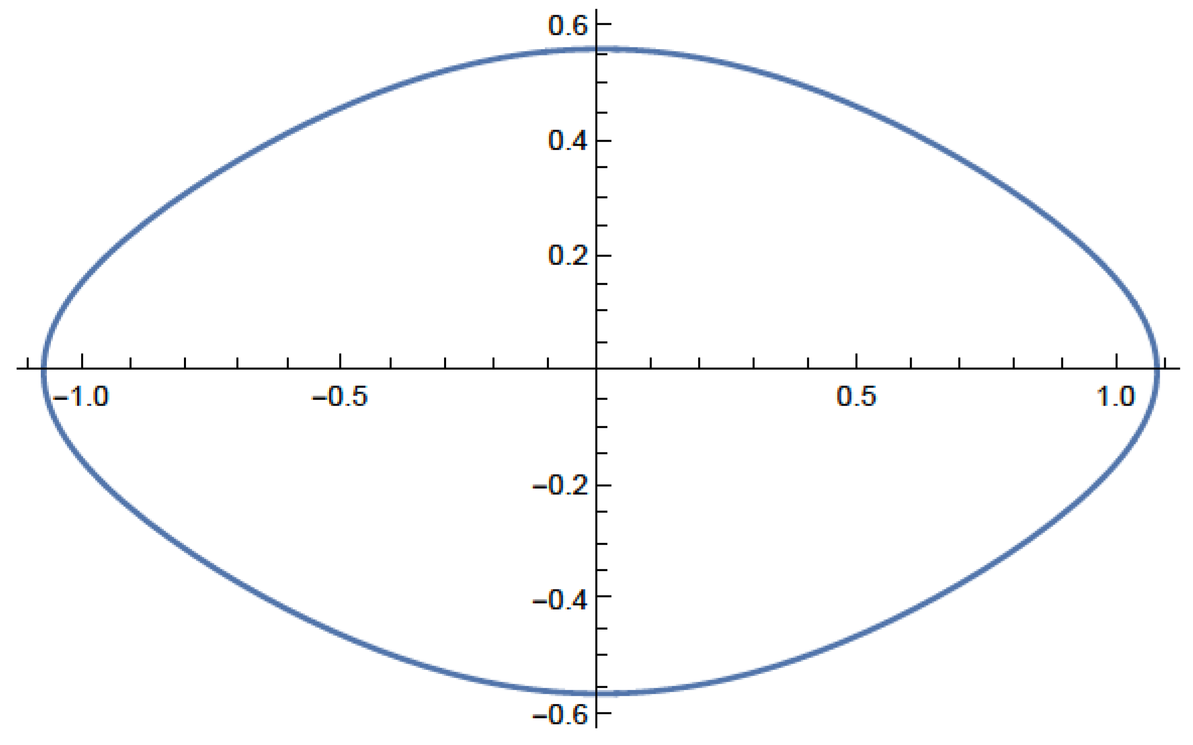
For the parameters a = 1, m = 1, and e = 0.1, the flat region is plotted in Figure 1(a) and a cross section is shown in Figure 1(b).
Figure 1.
(a) and (b). The flat region of the Kerr-Newman metric for the parameters a = 1, m = 1, and e = 0.1. The axes are (z, ρ). The surface is defined by r = e2/2m and the volume within this surface is empty and has a Minkowski metric. The flat region is, within the margin of error, bounded by the ring singularity at ρ = a = 1. Note the thinness of the flat region. The relationship between the Kerr-Newman flat region and its null Killing surface will play a role later. For comparison, here is a figure showing the Kerr null Killing surface for a > m. .
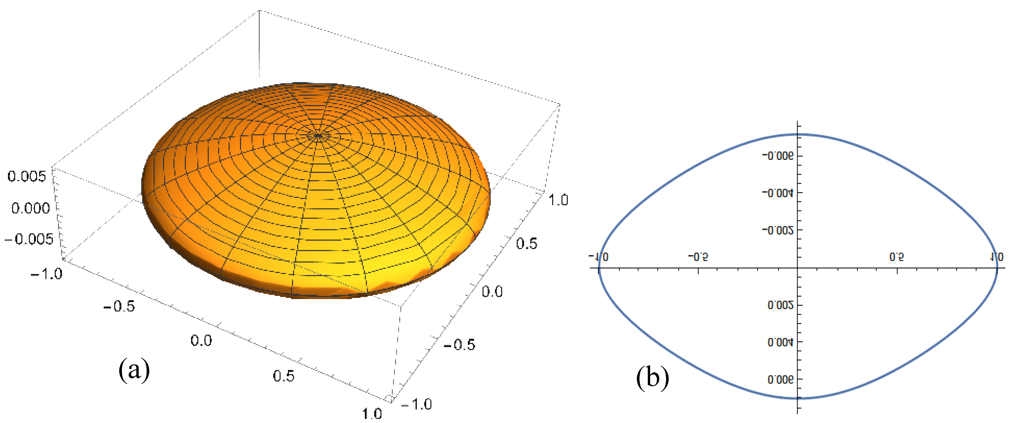
Figure 2.
The Kerr null Killing surface for a > m. Here m = 0.98 a. The ring singularity is at the cusp of the inner part of the surface.
Figure 2.
The Kerr null Killing surface for a > m. Here m = 0.98 a. The ring singularity is at the cusp of the inner part of the surface.
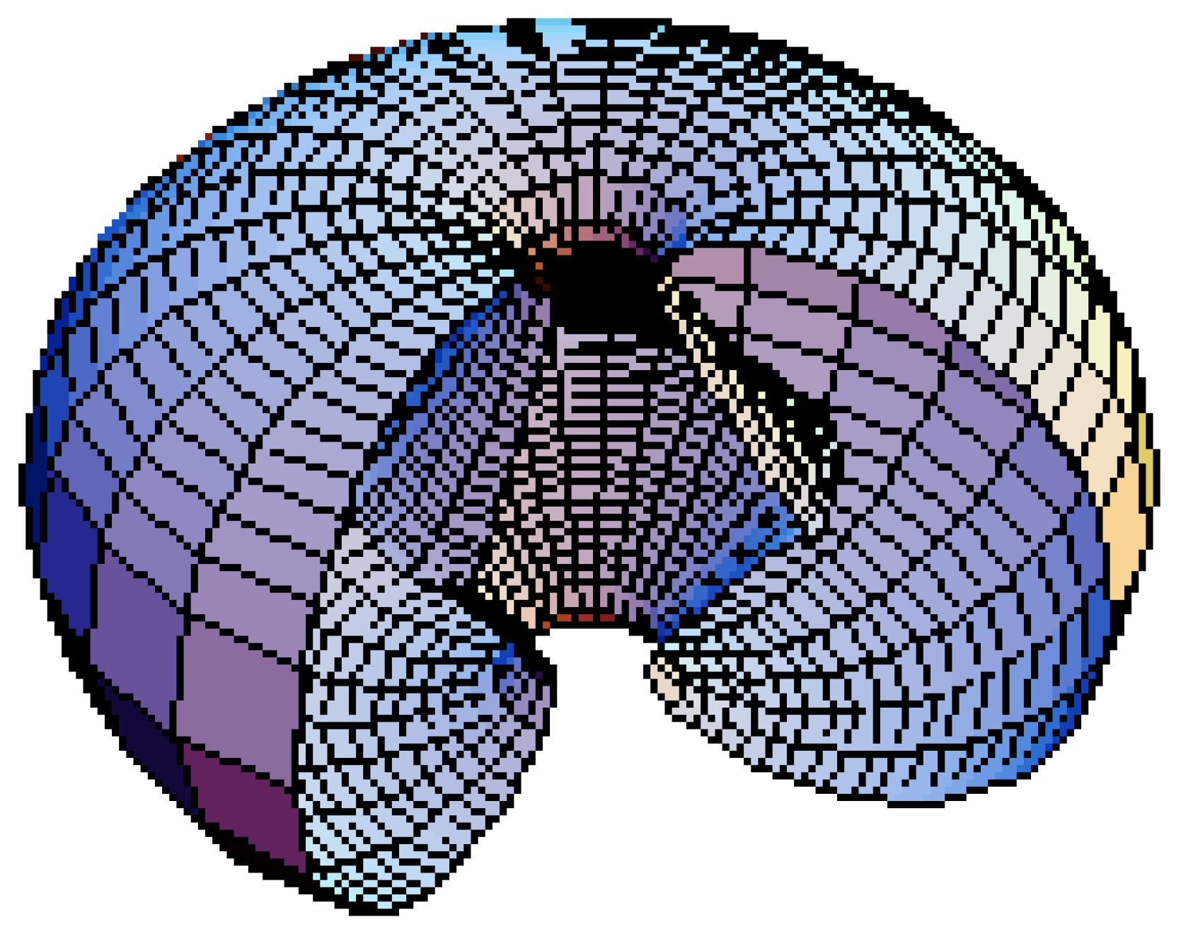
For the parameters, e = 0.1 and a = m = 1, the Kerr-Newman null Killing surface [2] is shown in Figure 3.
Figure 3.
The Kerr-Newman null Killing surfaces for e = 0.1 and a = m = 1. The inner surface does not terminate at the ring singularity but at a very slightly greater radius. This is not visible in the figure.
Figure 3.
The Kerr-Newman null Killing surfaces for e = 0.1 and a = m = 1. The inner surface does not terminate at the ring singularity but at a very slightly greater radius. This is not visible in the figure.
There are two important features of Figure 3 to note: the first is that a non-zero value of e opens up the surfaces at the poles allowing passage into the inner null surface, as is the case for the Kerr metric with a > m; and the second is that the inner surface does not terminate at the ring singularity, unlike the Kerr metric, but at a very slightly greater radius. This means that the ring singularity is directly reachable from outside the surfaces. In addition, what cannot easily be seen in Figure 3 is that there is a gap at the equator. This is shown in Figure 4.
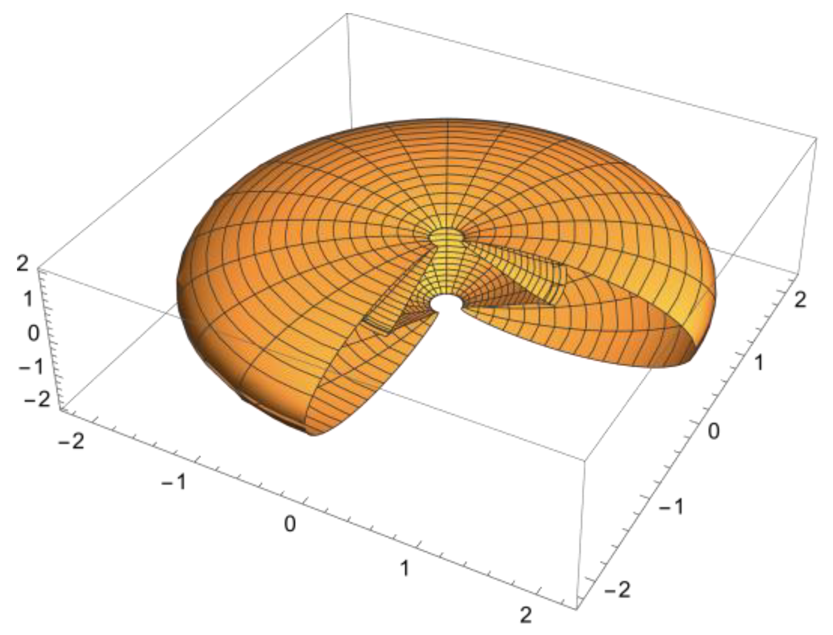
As the value of e increases, the gap in the null surfaces decreases, and when a2 + e2 > m2 and m > a > e the null surface changes its geometry to become a toroid. This is shown in Figure 5(a) and (b).
The gap seen in the inner part of the toroid shown in Figure 5 measures ~0.4. As pointed out above, the metric becomes that of flat Minkowski space for r = e2/2m. For the values of the parameters used to plot Figure 5, e2/2m ~0.4, which is what the gap measures in the figure.
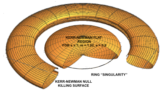
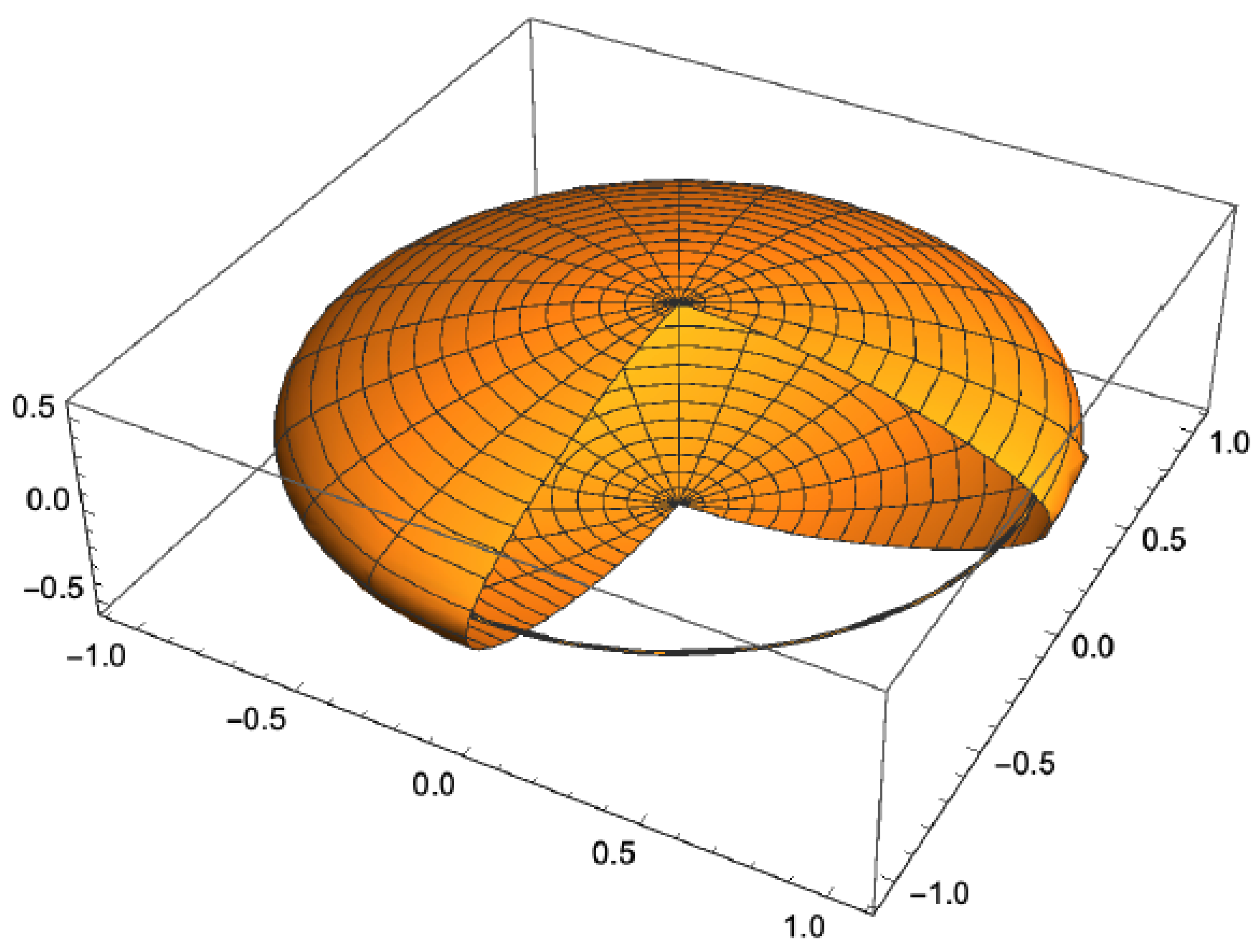
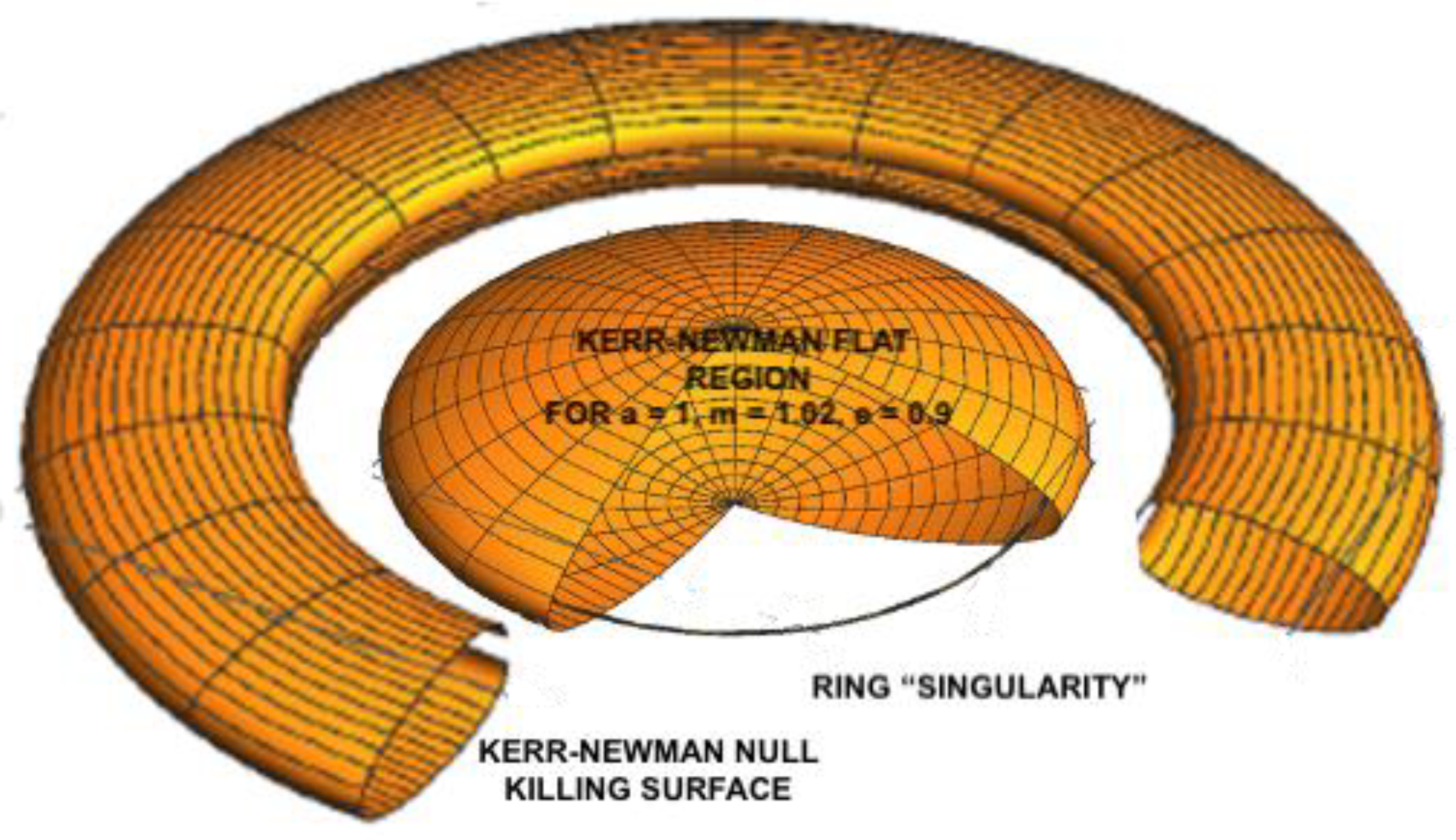
The Kerr-Newman flat region for a = 1, m = 1.02 and e = 0.9, implying that r = 0.397, has an extremely interesting feature. It is shown below in Figure 6 along with the ring “singularity” for ρ = a = 1.
Both Figure 5 and Figure 6 have the same values for the parameters a, m, and e so that Figure 6 is the flat region for the Kerr-Newman null Killing surface. The following is cross section of Figure 6.
Figure 7.
A cross section of the flat region shown in Figure 6. The “singularity” is at ρ = 1. Rotating this plot gives the 3-dimensional version shown with a cutout in Figure 6. .
For these parameters, the term “singularity” for the ring has been put in quotes since it is in the flat region of the solution. For the Kerr solution, the scalar polynomial Rabcd Rabcd diverges on the ring singularity so it is a real metric singularity. For the Kerr-Newman solution with the parameters above, the ring singularity has become a coordinate singularity since, if it were a real singularity, the space around it could not be flat. And since the “ring singularity” is enclosed by the flat region of the Kerr-Newman, were it a real singularity the space around it would have to become flat at r = e2/2m. This would appear to be impossible. The implication is that the mass, charge, and angular momentum associated with the Kerr-Newman solution cannot be attributed to the coordinate singularity.
What this explicitly shows is that the parameters m, e and a simply characterize the total mass, charge, and angular momentum associated with the solution. The location of energy in general relativity is an old problem, which was finally resolved by the realization that gravitational energy is not localizable. This differs from the Schwarzschild solution in that the Schwarzschild solution has a non-singular interior solution where one can at least localize the mass, but not the energy of the field itself. The Kerr-Newman solution, so far as I know, does not have a non-singular interior solution.
References
- C.A. López, “Extended model of the electron in general relativity”, Phys. Rev. D 30, pp. 313-316 (1984).
- G.E. Marsh, “Null-Killing Surfaces of the Kerr and Kerr-Newman Solutions of the Einstein Field Equations”, prepublication version available at http://www.gemarsh.com/wp-content/uploads/Null-Killing-Surf-of-the-Kerr-Kerr-Newman-Sol.pdf. Obtaining figures for the null Killing Surfaces shown in this paper requires extensive computation.
Figure 4.
An equatorial view of the Kerr-Newman null Killing surfaces for e = 0.1 and a = m = 1 showing the gap barely visible in Figure 3.
Figure 4.
An equatorial view of the Kerr-Newman null Killing surfaces for e = 0.1 and a = m = 1 showing the gap barely visible in Figure 3.
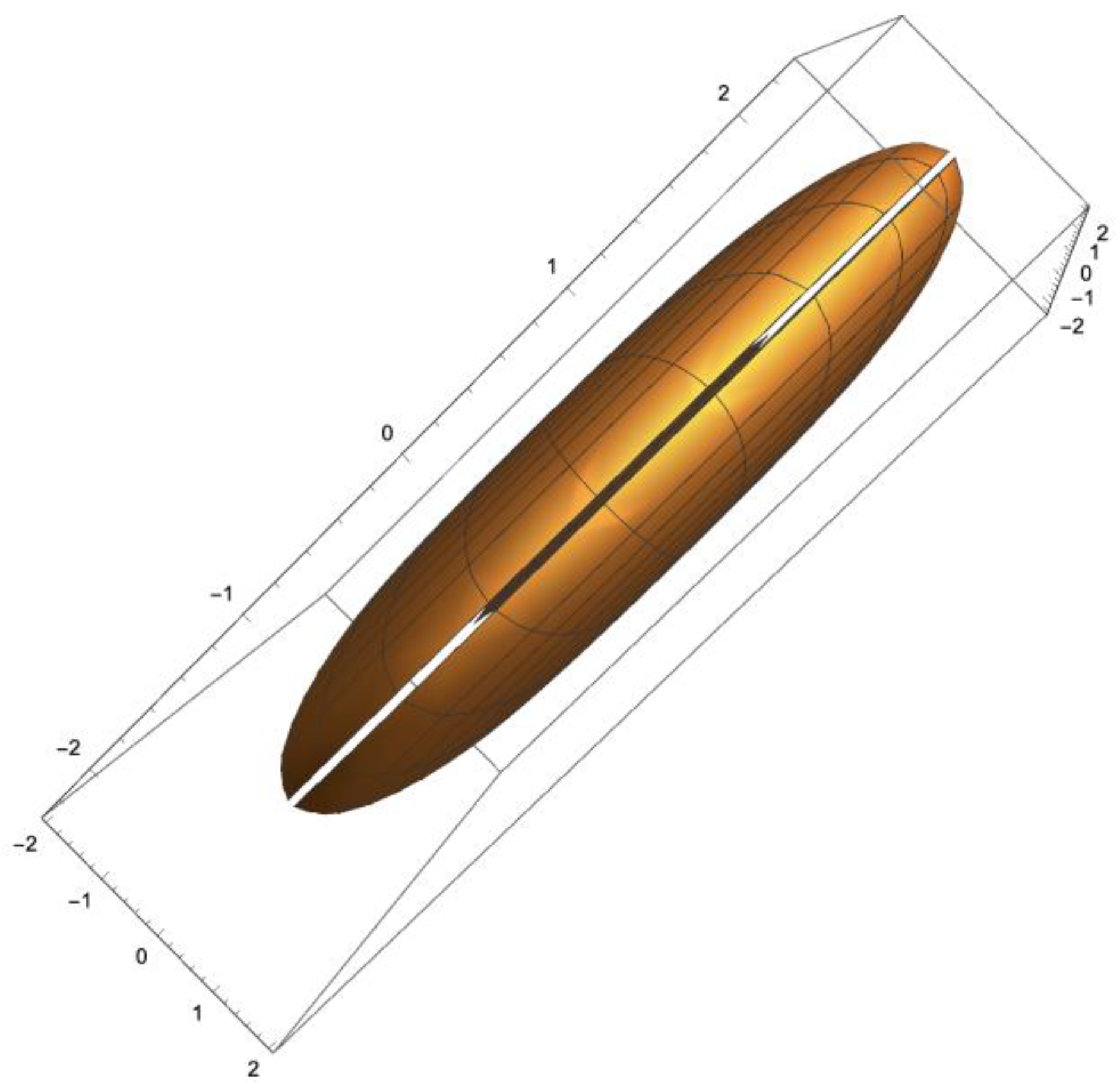
Figure 5.
(a) and (b). the Kerr-Newman null Killing surfaces for e = 0.9, a = 1, and m = 1.02. The ring singularity is outside the toroidal surface.
Figure 5.
(a) and (b). the Kerr-Newman null Killing surfaces for e = 0.9, a = 1, and m = 1.02. The ring singularity is outside the toroidal surface.
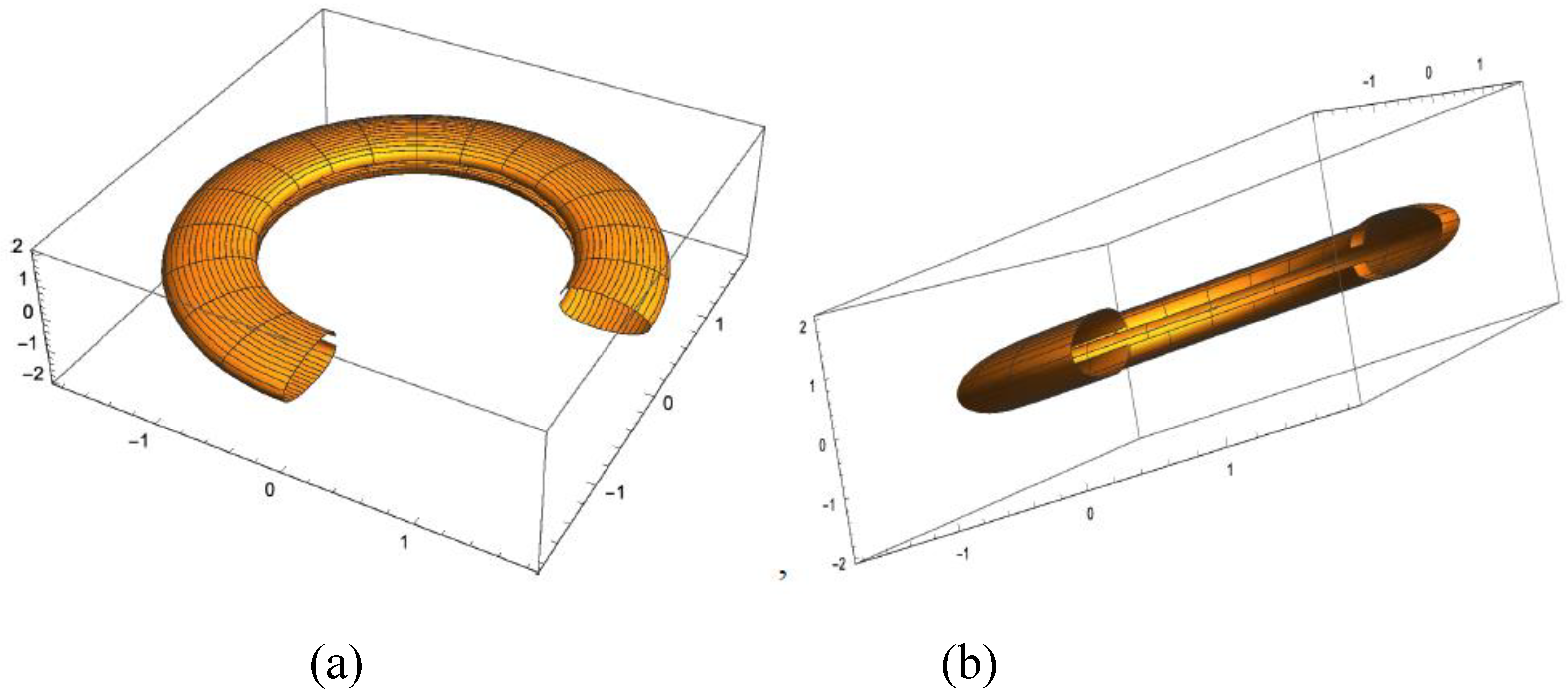
Figure 6.
The Kerr-Newman flat region with a cutout showing that for a = 1, m = 1.02 and e = 0.9. The ring “singularity” shown in the figure is at ρ = a = 1 and is clearly in the interior of the flat region.
Figure 6.
The Kerr-Newman flat region with a cutout showing that for a = 1, m = 1.02 and e = 0.9. The ring “singularity” shown in the figure is at ρ = a = 1 and is clearly in the interior of the flat region.
Disclaimer/Publisher’s Note: The statements, opinions and data contained in all publications are solely those of the individual author(s) and contributor(s) and not of MDPI and/or the editor(s). MDPI and/or the editor(s) disclaim responsibility for any injury to people or property resulting from any ideas, methods, instructions or products referred to in the content. |
© 2025 by the authors. Licensee MDPI, Basel, Switzerland. This article is an open access article distributed under the terms and conditions of the Creative Commons Attribution (CC BY) license (http://creativecommons.org/licenses/by/4.0/).
Copyright: This open access article is published under a Creative Commons CC BY 4.0 license, which permit the free download, distribution, and reuse, provided that the author and preprint are cited in any reuse.


