Submitted:
13 May 2025
Posted:
14 May 2025
Read the latest preprint version here
Abstract
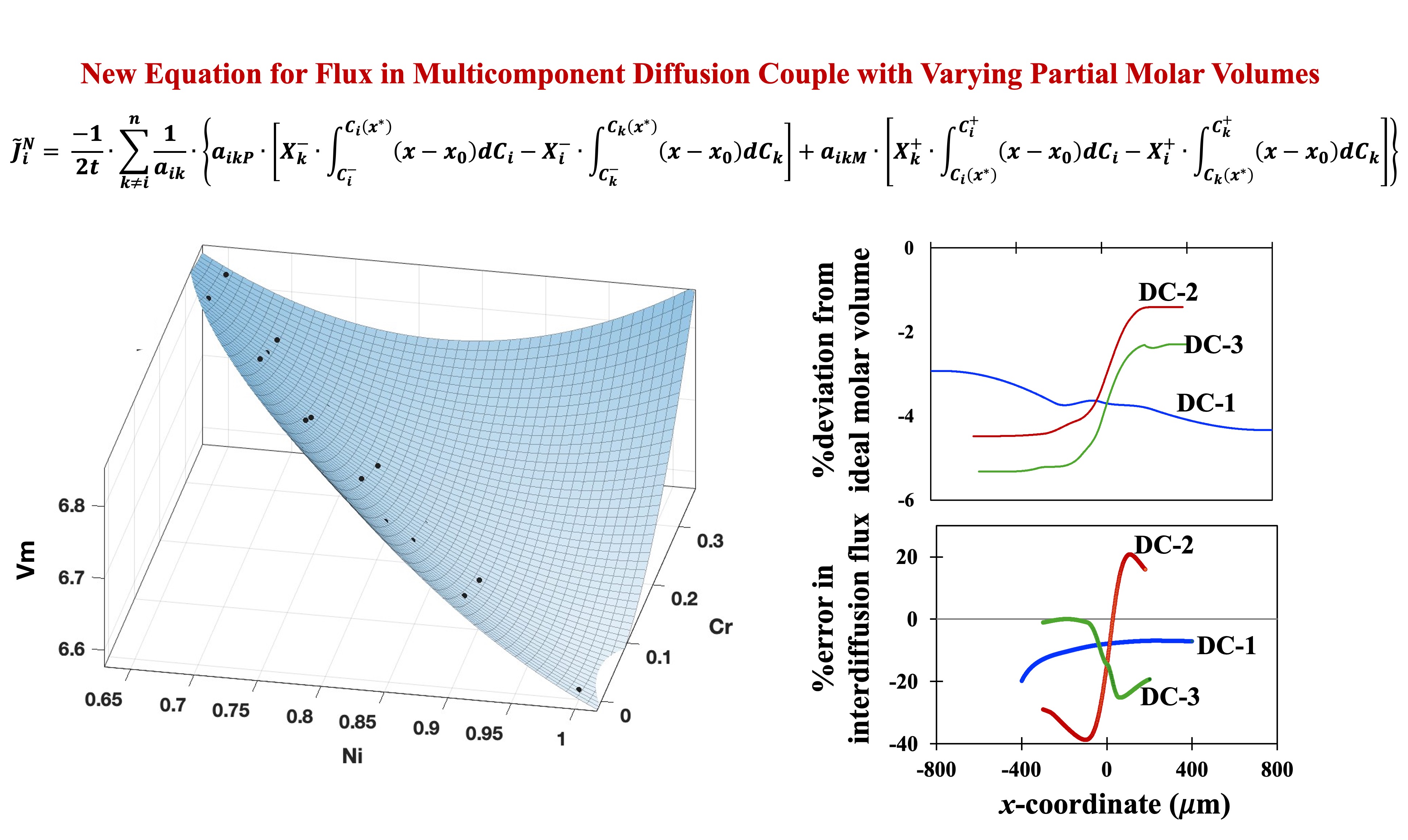
New equations are derived for determination of interdiffusion fluxes from experimental concentration profiles of multicomponent diffusion couples with composition dependent partial molar volumes of the diffusing components. The newly derived equations are applied to determine interdiffusion fluxes in experimental diffusion couples of FCC Ni-Cr-Al system. It is shown that for the case of varying partial molar volumes, the expressions discerned from the popular works of Sauer- Freise and Wagner are valid only for binary systems. Their use in determination of interdiffusion fluxes in ternary and higher order systems may lead to large errors; in the Ni-Cr-Al couple studied here, a mere 3% variation in deviation from ideality of molar volume is seen to give as high as -40% errors in interdiffusion fluxes, which may propagate to greater than 100% errors in interdiffusion coefficients determined from such fluxes. The newly derived expressions for fluxes in number fixed and volume fixed frames of reference are independent of the reference coordinate and they are also valid for multicomponent multiphase diffusion couples. In the absence of data on composition dependent molar volumes in ternary and higher order systems, the interdiffusion analysis so far has been carried out with assumption of constant molar volume. However, the newly developed equations in the present study and the observed large effect of molar volume on the flux analysis are expected to correct this trend.
Keywords:
interdiffusion
; flux
; molar volume
; frame of reference
1. Introduction
Experimental diffusion studies in multicomponent solids have so far been carried out with the assumption of constant partial molar volumes of components [1–16]. However, most of the real systems are non-ideal, in which case the partial molar volumes of individual components are dependent on composition. Thus, there is invariably a net volume change associated with the interdiffusion process. In a typical infinite diffusion couple, this leads to a non-zero velocity of the two terminal ends as well as a contribution to the interdiffusion flux at every plane in the diffusion couple from the non-Fickian drift associated with the volume change. This has been ignored so far due to the assumption of constant partial molar volume. Recent work by the present author [17,18] has highlighted the significance of considering composition dependent partial molar volumes in the interdiffusion analysis of experimental diffusion profiles developed in binary as well as multicomponent diffusion couples.
The method for extraction of interdiffusion coefficients from the experimental concentration profiles was first proposed by Boltzmann [19]. Matano first applied the Boltzmann’s analysis to solid-solid binary diffusion couple [20]. The crucial aspect of Matano’s analysis was the determination of the interdiffusion coefficients with respect to the location of initial contact plane, which in turn was determined with the simple mass balance. The method, which is popularly known as Boltzmann-Matano (BM) method, was primarily proposed for and applicable to binary systems and, for the assumption of constant molar volumes. Sauer and Freise [21] were the first ones to derive an expression for binary interdiffusion coefficients in terms of relative concentration variables as obtained from experimental diffusion profiles for composition dependent partial molar volumes. Wagner [22] and de Broeder [23] derived the similar equation for binary interdiffusion coefficient with different approaches. Various other authors [24–26] also attempted to address the problem of varying partial molar volumes, again, in binary interdiffusion analysis. A detailed review of all these methods is presented in [27]. The main success of Sauer-Freise [SF] equation [21] is that it does not need the location of the initial contact plane. However, the equation is applicable for binary analysis only. Roper and Whittle [28], without giving proper reasoning for the case of molar volume variation, proposed that the SF equation can be extended to even multicomponent systems.
Manning extensively worked on developing analytical relations between tracer diffusion coefficients and interdiffusion coefficients through the thermodynamic factors in multicomponent systems [29]. Manning’s model was applicable to the case of constant molar volume. Paul [30] has recently extended Manning’s model to include varying molar volumes. Manning’s model is essentially based on the assumption of random mixing of components, which means the binding energies and effect of neighboring atoms on jump frequencies are not considered. Most importantly, the model predictions of interdiffusion coefficients require the knowledge of thermodynamic factors as well as tracer diffusion coefficients at the desired composition. There are several restrictions on producing experimental tracer diffusivity data as it requires the use of radioactive isotopes. Although thermodynamic databases are now available for several systems, they are mostly based on extrapolating thermodynamic information from unary and binary (and in rare cases ternary) to higher order systems. Hence, the thermodynamic factors extracted from these have large errors, which are further propagated into predicted interdiffusion coefficients. Experimentally determined interdiffusion coefficients, on the other hand, inherently consist of all such contributions viz. vacancy wind effects, thermodynamic interactions and correlation effects. Hence, the experimental determination of interdiffusion coefficients from diffusion couple experiments currently has no matching alternative.
“Interdiffusion flux” is an important quantity in the phenomenological analysis of multicomponent diffusion. Dayananda [7,31] was the first one to emphasize the significance of flux determination from diffusion profiles. Dayananda and coworkers also developed various methodologies to utilize the fluxes in determining various phenomenological aspects of multicomponent diffusion including interdiffusion coefficients, average effective interdiffusion coefficients, diffusion depths and various constraints on the interdiffusion process [7,31–34]. Dayananda also provided a graphical proof for validity of SF equation to ternary and higher order systems but only for the assumption of constant molar volume [31]. So far, there is no attempt in the literature to check whether the expression for interdiffusion flux as discerned from SF or Wagner’s analysis is valid in the case of multicomponent diffusion with varying partial molar volumes. Still, it has been (wrongly) considered to be valid by numerous studies over the years. Hence, the objective of the present work is to analytically derive the expression for interdiffusion flux in a multicomponent diffusion couple with the composition dependent partial molar volumes. Earlier all such attempts were for binary systems only. However, the method used in the present study is valid in general for multicomponent systems with varying partial molar volumes. It is shown that the binary SF equation is not valid for multicomponent systems with composition dependent partial molar volumes. The newly derived equations are further applied to determine interdiffusion fluxes in three single-phase FCC Ni-Cr-Al diffusion couples reported in the literature [8,9].
2. Derivation of New Expression for Multicomponent Systems with Composition Dependent Partial Molar Volumes
2.1. Frame of Reference
In the interdiffusion analysis, it is of utmost importance to recognize and state the frame of reference that one is dealing with [35–38]. In a multicomponent system with composition dependent partial molar volumes, the continuity equation is applicable only in a stationary or lab-fixed frame of reference [35–38] and is expressed as.
where is the interdiffusion flux in moles/cm2-s measured with respect to the stationary frame (), is the concentration of the component i in moles/cm3, x is the distance coordinate and t is the time. Two of the most important frames of reference often used in the literature are the number fixed frame () and the volume fixed frame (). In , the fluxes are measured with respect to the local center of total number of moles of all components such that the net flux in number of moles per unit area per unit time is zero across all planes at all times [37]. In , the fluxes are measured with respect to the local center of total volume such that the net flux expressed in volume of the material is zero across all planes at all times [37]. The local center of number of moles and the local center of volume move with velocities and respectively, with respect to the stationary frame. Both and are functions of x and t.
By the definitions of and , the interdiffusion fluxes in these frames, and respectively, are constrained by the equations [35–38]:
and
where is the partial molar volume of the component i.
The interrelation between and can be written as
and that between and is given by
Summing Eq. (4) over all components, using constraint in Eq. (2) and knowing the relation for molar volume (),
one can write [35–37]
Similarly, multiplying Eq. (5) with , then summing it over all components, using Eq. (3) and knowing the relation,
one can write [35–38]
Substituting for from Eq. (7) into Eq. (4),
However,
where, denotes the mole fraction of i.
Thus, we get
Similarly, from Eq. (5) and (9), one obtains
Eqs. (12) and (13) will be used in further analysis to get expressions for and as determined directly from the experimental concentration profiles of a multicomponent diffusion couple.
2.2. Component Velocities and Fluxes at the Terminal Ends of a Diffusion Couples
In an infinite diffusion couple, the compositions at the two terminal ends are unaffected. Thus, the interdiffusion fluxes in and are zero in the two terminals, where the composition gradients are zero. However, in a non-ideal system, which most systems are, the partial molar volume of a component changes with composition and hence, the diffusion is associated with a net volume change, leading to net motion of each terminal end. Thus, the interdiffusion fluxes measured in are not zero in the two terminals. Let and denote the concentrations of component i in the left and right terminal alloys, respectively. In each of the terminals, the interdiffusion fluxes () of the individual components are constant. Also, the average atom velocity should be same for all components in each terminal [22]; let them be and in the left and the right terminals respectively. Let and denote the interdiffusion fluxes of components i and k in in the left terminal alloy. Since, and , one can write for any two given components i and k,
Based on Eq. (11), multiplying both sides of Eq. (14a) by , the molar volume of left terminal alloy, one can also write
where, and are mole fractions of components i and k respectively in the left terminal alloy.
Similarly, in the right terminal alloy, with and being the mole fractions of i and k in it, one can write
The significance of Eqs. (14 a-b) and (15 a-b) will be clearer in the analysis to follow.
2.3. Interdiffusion Flux in Number Fixed Frame in Terms of Molar Concentrations
In an infinite diffusion couple, a given composition is a function of the Boltzmann parameter [19] λ, which is given by
where, is the reference plane in a stationary frame, which is typically considered to be the initial weld plane. Thus, Eq. (1) can be written as
Substituting for and based on Eq. (16) we get
Integrating Eq. (18) between and the desired location x in the diffusion zone at a fixed time t,
where, and are the interdiffusion fluxes in R0 at and at x respectively. Similarly, we can write for any other Component k,
Multiplying Eq. (19a) by and subtracting Eq. (19b) multiplied by from it,
However, the term in second square bracket on right hand side of Eq. (20) is zero on account of Eq. (14b). Thus, one can write
On a similar line, integrating Eq. (18) between x and , we get for components i and k respectively,
Multiplying Eq. (22a) by and subtracting Eq. (22b) multiplied by from it,
However, the term in second square bracket on right hand side of Eq. (23) is zero on account of Eq. (15b). Thus, one can write
Let, denote the concentration of a component i at the desired location . Now, multiplying Eq. (21) by and adding Eq. (24) multiplied by to it one obtains,
provided , where,
The mathematical treatment applied from Eq. (19a) through Eq. (28) can also be extended to any pair of component i and any component m other than i and k to get
provided . Summing all such equations written for each pair of the component i and a component k other than i, i.e. Eq (25a), (25b) etc., and using Eq. (12), one can write,
provided any of . Eq. (29) gives an exact expression for interdiffusion flux measured in number fixed frame in a multicomponent diffusion couple with composition dependent partial molar volumes.
2.4. Interdiffusion Flux in Volume Fixed Frame in Terms of Molar Concentrations
Based on Eq. (11), Eq. (25a) and (25b) can be written as
Multiplying (30a) by and adding to it (30b) multiplied by ,
Thus, writing Eq. (30a) for each pair of the component i and a component k other than i, multiplying throughout by and then summing them all and, using Eq. (13), we get
Eq. (32) gives an exact expression for interdiffusion flux measured in volume fixed frame in a multicomponent diffusion couple with composition dependent partial molar volumes.
2.5. Interdiffusion Fluxes ( and ) in Terms of Relative Concentration Variables
In terms of , the expression for i.e. Eq. (29) can be reduced to the form
where, and provided, any of the . The derivation of Eq. (34) from Eq. (29) is presented in Supporting Data File. On a similar line, it can be shown that the expression for , Eq. (32), can be reduced to the form
provided, any of the . It should be noted that Eq. (29) and (32) are equivalent to Eq. (34) and (35) respectively. Eq. (34) and (35) are independent of the coordinate system used for the analysis. Hence, Eq. (29) and (32) are also independent of the coordinate system. Thus, x0 in Eq. (29) and (32) can be replaced with any convenient coordinate in the experimental diffusion profiles.
2.6. Interdiffusion Fluxes for Binary Systems
In a binary system of component 1 and 2, it can be easily shown that (say) and that the determinants in Eq. (29) reduce to the form , and . Thus, Eq. (29) for a binary system reduces to
Eq. (36) and (37) show that as expected in a binary system. Further, Eq. (34) and (35) can be shown to reduce for a binary system to
It should be noted that Eq. (36) and (38) are equivalent. Also, the factor of should not be ignored that is required for converting binary interdiffusion flux from to as observed from Eq. (38) and (39). Although Sauer and Freise [21] and Wagner [22] did not explicitly list the equation for interdiffusion flux, the equation that can be discerned from the one proposed for interdiffusion coefficient by them is similar to Eq. (38) in RN or Eq. (39) in RV. We will refer to Eq. (38) as SF equation as it has often been suggested to be valid for multicomponent systems too [7,28]. However, the analysis presented here clearly shows that the SF equation is not valid for ternary and higher order systems exhibiting composition dependent partial molar volumes. Based on Eq. (38) and (39), it is easily discerned that the binary interdiffusion coefficient as suggested by Eq. (14) of Wagner [22], corresponds to the volume fixed frame of reference. For the assumption of constant molar volume though, Eq. (38) and (39) are identical because all partial molar volumes are constant and equal to molar volume of the alloy.
2.7. Case of Constant Partial Molar Volumes
In the absence of data on partial molar volumes as functions of compositions in multicomponent systems, they are generally assumed constant for multicomponent diffusion analysis. In case of constant partial molar volumes, there is no net change in the volume after diffusion and hence, the two terminal ends do not move with respect to the stationary frame. Thus, both the number fixed frame and volume fixed frame coincide with the stationary frame leading to (say) at any plane in an infinite diffusion couple. Since the interdiffusion fluxes at the two terminals i.e. and are zero, Eq. (19a) and (22a) can simply be written as
Eq. (40) matches with the one derived by Dayananda and Kim [7] and the superscript CV in denotes that it is applicable for the assumption of constant partial molar volume.
Further, it can be shown that (only) for the assumption of constant partial molar volumes, both Eq. (34) and (35) can reduce to
It should be noted here that Eq. (40) and (41) are valid in a multicomponent system but only for the assumption of constant partial molar volumes. For composition dependent partial molar volumes, the correct equations for interdiffusion fluxes in multicomponent systems are those given by Eq. (29) and (34) in RN and, by Eq. (32) and (35) in RV.
3. Application of New Equations to Determination of Interdiffusion Fluxes in Ni-Cr-Al Diffusion Couples
For applying the newly developed equations in the present work to a multicomponent system, it is essential to have extensive data on lattice parameters as function of composition available in the system. This would enable the determination of the molar volumes at various compositions as desired in the equations. Additionally, there should be data on diffusion profiles available in the literature. Ni-Cr-Al is one of the very few systems in which both the desired data are available and hence, it is used for demonstrating the application of newly developed equations in the present work.
The lattice parameters in FCC phase of the ternary Ni-Cr-Al systems were taken from the work of Taylor and Floyd [39] as summarized in [40]. The molar volumes were determined from the lattice parameters at several different compositions of the FCC phase and were fitted to a quadratic equation in the ternary composition space () as
where, is in cm3/mol and and are mole fractions of Ni and Cr respectively. The tabular data on the molar volumes at various compositions and the 3-D plots of the molar volume versus composition based on Eq. (42) are presented in Table S1 and Figure S1 respectively of Supporting Data File. The partial molar volumes of the individual components were evaluated as functions of compositions from Eq. (42) with the procedure outlined by the present author in a recent work [18] and the supplementary file therein.
Nesbitt and Heckel [8,9] extensively worked on the interdiffusion analysis in FCC Ni-Cr-Al system by utilizing solid-solid infinite diffusion couples. However, all their analysis was based on the assumption of constant molar volume. The experimental data from three of their reported diffusion couples were used in the present work for determination of interdiffusion fluxes by the application of the newly developed equations. The designations of the diffusion couples, their terminal alloy compositions, isothermal annealing temperatures and time as listed by Nesbitt and Heckel are presented in Table 1.
The concentration data for the three couples (DC-1, DC-2 and DC-3) were extracted from the concentration profiles presented by Nesbitt and Heckel [8,9] by using a digital data-extraction software, DigitizeIt. The concentration data were then fitted with the computer program MultiDiFlux, the working of which has been explained in various earlier works [14,16,41]. The fitted concentration profiles of the couples DC-1, DC-2 and DC-3 are presented in Figures 1(a), 2(a) and 3(a) respectively. The interdiffusion fluxes in number fixed frame as determined using the newly derived equation, Eq. (29) are presented as solid lines for the three couples in Figures 1(b), 2(b) and 3(b) respectively. Similarly, the interdiffusion fluxes in volume fixed frame as determined using the newly derived equation Eq. (32) are presented in Figures 1(c), 2(c) and 3(c) as solid lines. The interdiffusion fluxes as determined by the Sauer-Friese equation, Eq. (38), which has been shown here to be not correct for multicomponent systems with varying partial molar volumes, are shown as dashed lines for a comparison. It can be seen from Figure (1b) that the values of as determined from the newly developed equation, Eq. (29) are almost similar to those determined by S-F equation, Eq. (38) for all three components in DC-1. However, Figures 2 (b) and 3 (b) show that, in DC-2 and DC-3, the two sets of values show large differences, especially for Ni and Al. A similar trend is observed from Figures 1 (c), 2 (c) and 3 (c) for comparison of as determined from the newly developed equation, Eq. (32) and the flux determined form S-F equation, Eq. (38) with the differences being slightly larger for than for . This is a critical observation as it shows that the S-F analysis is generally valid for determining interdiffusion fluxes only in the systems with constant molar volumes. Its use for determining interdiffusion fluxes, in the multicomponent systems with composition dependent partial molar volumes should lead to errors in estimation of the fluxes. Such errors would be further propagated when the fluxes are used for evaluating interdiffusion coefficients leading to larger errors in the values of the latter.
Figure 1.
(a) Fitted concentration profiles developed in Couple DC-1. (b) Interdiffusion flux profiles in as determined by newly developed Eq. (29) shown as solid lines. (c) Interdiffusion flux profiles in as determined by newly developed Eq. (32) shown as solid lines. In (b) and (c) the dashed lines show the fluxes determined by SF equation Eq. (38).
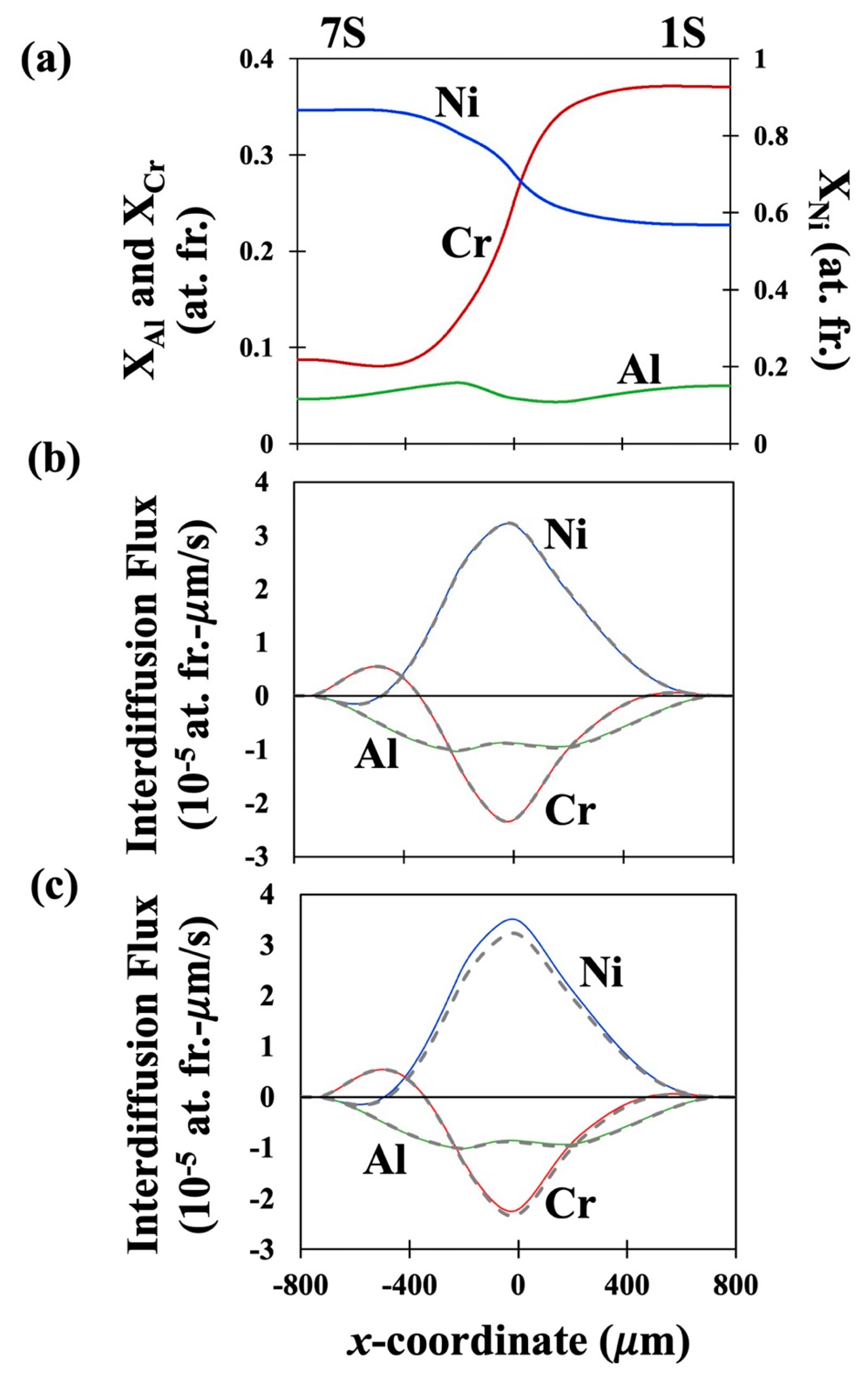
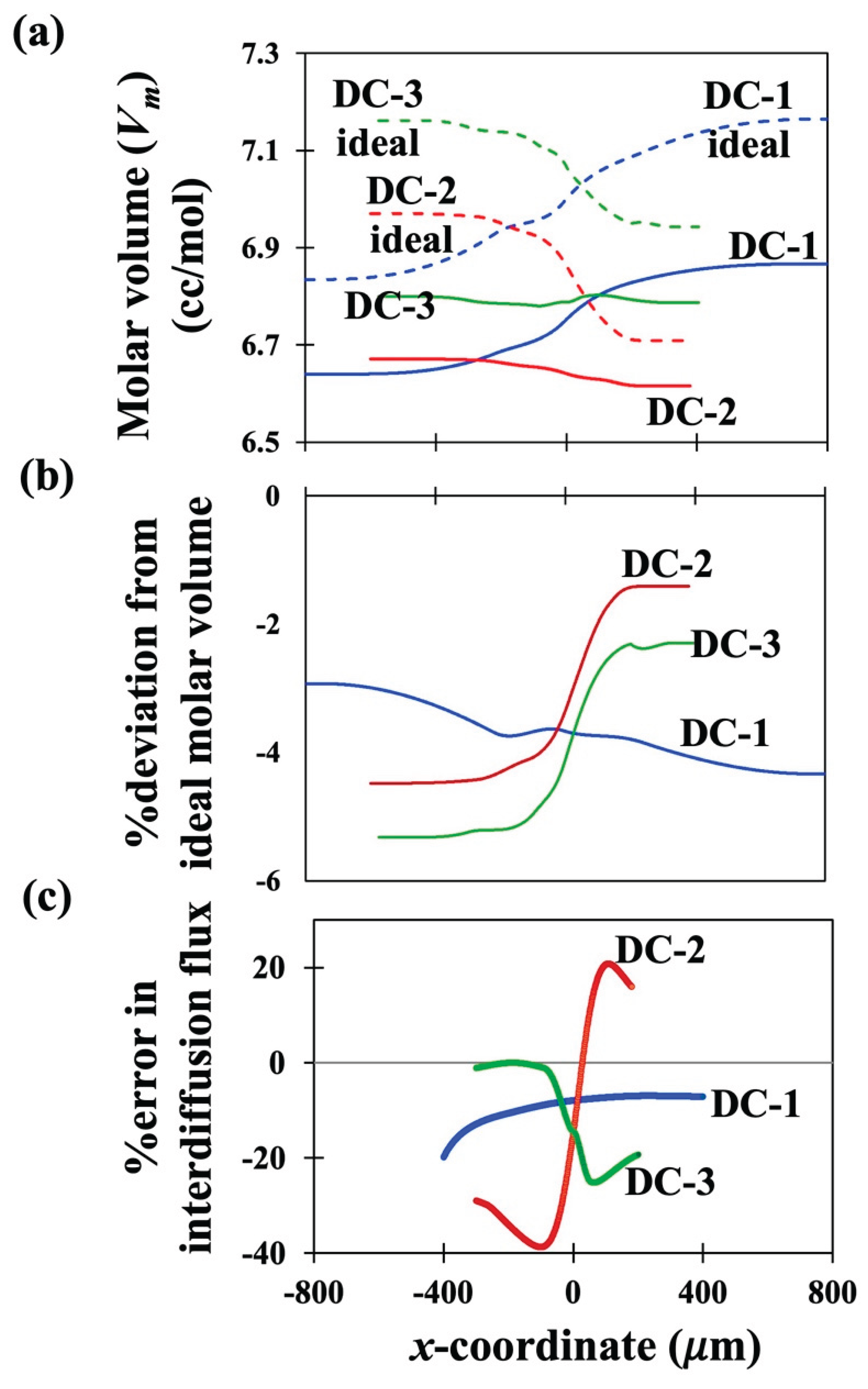
Figure 4 (a) presents the variation of molar volumes in the diffusion zones of the three couples DC-1, DC-2 and DC-3 as represented by solid lines. Variation of ideal molar volume is also shown on Figure 4 (a) by dashed lines for the three couples. The deviation of the actual molar volume from ideal values (in %) is shown for all three couples in Figure 4 (b). Figure 4 (c) presents the errors in the evaluation of interdiffusion fluxes of Ni, if determined by S-F formula, Eq. (38) over the correct formula, Eq. (32) derived in this work for all three couples.
Only Ni-fluxes are presented in Figure 4 (c) because Ni is seen to exhibit the largest errors of all three components. Since the errors involved with the end regions where the concentration gradients are approaching zero are generally large, only the errors in fluxes in the central part of the diffusion zones are presented in Figure 4 (c). It can be qualitatively seen that the errors in the fluxes are larger for a given couple, if the variation of deviation from ideal molar volume in the diffusion zone of the couple is larger. Figure 4 (a) shows that the molar volume for Couple DC-1 varies almost parallelly with the variation shown by its ideal molar volume. Thus, in Figure 4 (b), the overall variation in deviation from ideal molar volume varies by small amount (~1.4% points) over the diffusion zone. However, variation in deviation from ideality for the molar volumes of DC-2 and DC-3 in their respective diffusion regions is ~3.1 and 3 % points respectively. Correspondingly, the errors in fluxes are largest for DC-2 followed by DC-3 and the smallest for DC-1. It is interesting to note that the overall variation of molar volume is highest in DC-1 but the deviation from ideality is lowest for DC-1. On the other hand, DC-2 and DC-3 show much lesser overall variation in the molar volume but their deviation from ideality is larger. Thus, the deviation of the molar volume from ideal molar volume plays the most dominant effect in determining the local interdiffusion fluxes than the absolute variation in molar volume within the diffusion zone. This highlights the necessity of the newly derived equations for interdiffusion analysis of multicomponent diffusion couples exhibiting composition dependent partial molar volumes.
4. Discussion
The newly developed equations, Eq. (29) and (34), are the exact expressions for interdiffusion flux of a component with respect to the number fixed frame and Eq. (32) and (35) are those for the interdiffusion fluxes with respect to volume fixed frame as determined from experimental concentration profiles of a multicomponent diffusion couple with composition dependent partial molar volumes. By definition, Eq. (29) gives the interdiffusion flux with respect to the local center of number of moles and Eq. (32) gives that with respect to the local center of volume. Thus, both these equations are naturally independent of the reference coordinate (x0) used for the analysis. Moreover, since the variation in molar volume is accounted for, the equations are also applicable for the analysis of multicomponent multiphase diffusion couples.
The most significant outcome of the present work is that it proves that the popular SF equation for varying partial molar volumes is applicable only for binary interdiffusion analysis and its use, as it is, in the analysis of multicomponent systems leads to errors in the determination of fluxes. This is against the popular belief otherwise. In the Ni-Cr-Al couples studied here, it is observed that a mere 3-4% variation in deviation of molar volume from ideality leads to errors of -40 to 20% in the interdiffusion fluxes; see Figure (4). A rough estimate, as described in Supporting Data File, suggests that this would further propagate to more than 100% errors in interdiffusion coefficients evaluated from these fluxes if errors in all the fluxes add up. On the other hand, for small variations of molar volumes in the diffusion zone, the fluxes evaluated by the binary SF equation, Eq. (38) are almost similar to those evaluated based on constant molar volume, Eq. (41). A comparison in this regard for the three studied couples is presented in Figure 2S of Supporting Data File. Thus, the use of binary SF equation, Eq. (38) to determination of fluxes in ternary and higher order systems is akin to the assumption of the constant molar volumes, at least in couples with not too large variations in molar volumes. This shows that the variation in partial molar volumes should not be ignored in the interdiffusion analysis of the multicomponent diffusion couples and that only the newly developed equations here must be used for the accurate analysis. This also calls for an urgent need for experimental determination of molar volumes as functions of compositions in various multicomponent systems; this point is also highlighted through the present author’s previous works [17,18].
With the increasing demand for accurate experimental data for use in advanced technology development such as artificial intelligence (AI), machine learning (ML) and integrated computational materials engineering (ICME), considering composition-dependent molar volumes in multicomponent interdiffusion analysis is the need of the hour. However, there have been lack of such analysis so far, because of both the lack of experimental data on molar volumes in multicomponent systems and the lack of appropriate equations that can account for varying partial molar volumes while analyzing interdiffusion in multicomponent couples. Thus, the newly developed equations in the present work are expected to pave the way for detail experimental investigations of molar volumes of multicomponent systems as functions of compositions and to have a phenomenal impact on the experimental interdiffusion analysis of the multicomponent diffusion couples.
5. Conclusions
In the absence of the data on molar volumes as functions of compositions in the multicomponent systems, the analysis of experimental concentration profiles developed in a multicomponent diffusion couple for interdiffusion fluxes and coefficients has so far been carried out in the literature with the assumption of constant molar volume. However, it has been, albeit wrongly, generally suggested, without any analytical work, that the binary SF equations Eq. (38) can straight be used for ternary and higher order systems with composition dependent partial molar volumes to determine the interdiffusion fluxes in multicomponent diffusion couples. In the present work, new equations are derived for determination of interdiffusion fluxes from experimental concentration profiles of multicomponent diffusion couples. Application of the newly developed equations to diffusion couples in FCC Ni-Cr-Al system shows that a mere 3% variation in deviation from ideality of the molar volume in the diffusion zone may lead to about 40% errors in fluxes if assumption of constant molar volume is employed or if the SF equation proposed for binary diffusion is used. This may further translate to more than 100% errors in the interdiffusion coefficients determined from such fluxes. This emphasizes the need for development of databases for molar volumes in multicomponent systems and also, the necessity of the use of the newly developed equations in interdiffusion analysis of the multicomponent diffusion couples with varying partial molar volumes. The newly developed equations are independent of the reference coordinate used i.e. they do not need the location of the initial contact plane and, they are also applicable for the analysis of multicomponent multiphase diffusion couples.
Supplementary Materials
The following supporting information can be downloaded at the website of this paper posted on Preprints.org.
Acknowledgement
This work is financially supported by internal grants of IIT Kanpur.
References
- L. S. Darken; “Diffusion, Mobility and Their Interrelation through Free Energy in Binary Metallic Systems”; Transactions of AIME; Vol. 175; 1948; pp. 184-201.
- L. S. Darken; “Formal Basis of Diffusion Theory” in Atom Movements; ASM, Cleveland, Ohio; 1951; pp. 1-25.
- J. S. Kirkaldy, J. E. Lane and G. R. Meson; “Diffusion in Multicomponent Metallic Systems VII. Solutions of the Multicomponent Diffusion Equations with Variable Coefficients”; Canadian Journal of Physics; Vol. 41; 1963; pp. 2174-2186.
- J. S. Kirkaldy and J. E. Lane; “Diffusion in Multicomponent Metallic Systems IX. Intrinsic Diffusion Behavior and Kirkendall Effect in Ternary Substitutional Solutions”; Canadian Journal of Physics; Vol. 44; 1966; pp. 2059-2072.
- P. T. Carlson, M. A. Dayananda and R. E. Grace; “Diffusion in Ternary Ag-Zn-Cd Solid Solutions”; Metallurgical Transactions; Vol. 3; 1972; pp. 819-826.
- T. D. Moyer and M. A. Dayananda; “Diffusion in β2 Fe-Ni-Al Alloys”; Metallurgical Transactions A; Vol. 7A; 1976; pp. 1035-1040.
- M. A. Dayananda and C. W. Kim; “Zero Flux Planes and Flux Reversals in Cu-Ni-Zn Diffusion Couples”; Metallurgical Transactions A; Vol. 10A; 1979; pp. 1333-1339.
- J. A. Nesbitt and R. W. Heckel; “Interdiffusion in Ni-Rich Ni-Cr-Al Alloys at 1100 and 1200 °C: Part I. Diffusion Paths and Microstructures”; Metallurgical Transactions A; Vol. 18A; 1987; pp. 2061-2073.
- J. A. Nesbitt and R. W. Heckel; “Interdiffusion in Ni-Rich Ni-Cr-Al Alloys at 1100 and 1200 °C: Part II. Diffusion Coefficients and Predicted Concentration Profiles”; Metallurgical Transactions A; Vol. 18A; 1987; pp. 2075-2086.
- R. Bouchet and R. Mevrel; “A Numerical Inverse Method for Calculating the Interdiffusion Coefficients Along a Diffusion Path in Ternary Systems”; Acta Materialia; Vol. 50; 2002; pp. 4887-4900.
- M. S. A. Karunaratne and R. C. Reed; “Interdiffusion of the Platinum Group Metals in Nickel at Elevated Temperatures”; Acta Materialia; Vol. 51; 2003; pp. 2905-2919.
- L. R. Ram-Mohan and M. A. Dayananda; “A Transfer Matrix Method for the Calculation of Concentrations and Fluxes in Multicomponent Diffusion Couples”; Acta Materialia; Vol. 54; 2006; pp. 2325-2334.
- M. A. Dayananda; “A Direct Derivation of Fick’s Law from Continuity Equation for Interdiffusion in Multicomponent Systems”; Scripta Materialia; Vol. 210; 2022; pp. 114430.
- V. Verma, A. Tripathi, T. Venkateswaran, K. N. Kulkarni; “First Report on Entire Sets of Experimentally Determined Interdiffusion Coefficients in Quaternary and Quinary High-Entropy Alloys”; Journal of Materials Research; Vol. 35 (2); 2020; pp. 162-171.
- Vivek Verma and Kaustubh N. Kulkarni; “Square Root Diffusivity Analysis of Body-Diagonal Diffusion Couples in FeNiCoCr quaternary and FeNiCoCrMn quinary systems”; Journal of Phase Equilibria and Diffusion; 43 (6); 2022; pp. 903-915.
- G. P. S. Chauhan and Kaustubh N. Kulkarni; “Investigations of Ternary Interdiffusion in β-(BCC) Phase Field of Ti-Al-Mo System”; Metallurgical and Materials Transactions A; Vol. 52A; 2021; pp. 413-425.
- Kaustubh N. Kulkarni; “Derivation of expressions for interdiffusion and intrinsic diffusion flux in presence of chemical potential gradient in a multicomponent system with composition dependent molar volume”; Oxford Open Materials Science; 3 (1); 2023; itad018.
- Kaustubh N. Kulkarni; “Velocity of Volume Fixed Frame and Its Application in Simulating Concentration Profiles in Multicomponent Diffusion”; Journal of Phase Equilibria and Diffusion; 45 (4); 2024; pp. 757-763.
- L. Boltzmann; “Zur Integration der Diffusionsgleichung bei variable Diffusionscoefficienten”; Annual Review of Physical Chemistry; Vol. 53; 1894; pp. 959-964.
- C. Matano; “On the Relation between Diffusion-Coefficients and Concentrations of Solid Metals (The Nickel-Copper System)”; Japanese Journal of Physics; Vol. 8; 1935; pp. 109-113.
- F. Sauer and V. Freise; “Diffusion in binären Gemischen mit Volumenänderung”; Vol. 66 (4); 1962; pp. 353-362.
- C. Wagner; “The Evaluation of Data Obtained with Diffusion Couples for Binary Single-Phase and Multiphase Systems”; Acta Metallurgica; Vol. 17; 1969; pp. 99-107.
- F. J. A. den Broeder; “A General Simplification and Improvement of the Matano-Boltzmann Method in the Determination of the Interdiffusion Coefficients in Binary Systems“; Scripta Materialia; Vol. 3; 1969; pp. 321-326.
- R. Balluffi; “On the Determination of Diffusion Coefficients in Chemical Diffusion”; Acta Metallurgica; Vol. 8; 1960 pp. 871–873.
- A.G. Guy, R.T. DeHoff, and C. Smith; “Calculation of Interdiffusion Coefficients Considering Variations in Atomic Volume”; ASM Transactions Quarterly; Vol. 61; 1968; pp. 314–20.
- M. Danielewski and H. Leszczynski; “Generalization of Matano’s Method: Interdiffusion in Solutions with Volume Change”; International Journal of Mathematical Analysis; Vol. 9 (30); 2015; pp. 1463–1476.
- A. Tripathi and K. N. Kulkarni; “Effect of Varying Molar Volume on Interdiffusion Analysis in a Binary System”; Metallurgical and Materials Transactions A; Vol. 52A; 2021; pp. 3489-3502.
- G. W. Roper and D. P. Whittle; “Interdiffusion in Ternary Co-Cr-Al Alloys”; Metal Science; Vol. 14 (1); 1980; pp. 21-28.
- J. R. Manning; “Cross Terms in the Thermodynamic Diffusion Equations for Multicomponent Alloys”; Metallurgical Transactions; Vol. 1; 1970; pp. 499-505.
- A. Paul; “Effect of Molar Volume of Diffusing Elements and Cross Terms of Onsager Formalism (Vacancy Wind Effect) on Estimated Diffusion Coefficients in Ternary and Multicomponent Solid Solutions”; Materialia; Vol. 40; 2025; 102400. [CrossRef]
- M. A. Dayananda; “An analysis of Concentration Profiles for Fluxes, Diffusion Depths, and Zero Flux Planes in Multicomponent Systems”; Metallurgical Transactions A; Vol. 14A; 1983; pp. 1851-1858.
- M. A. Dayananda and D. A. Behnke; “Effective Interdiffusion Coefficients and Penetration Depths”; Scripta Materialia; Vol. 25; 1991; pp. 2187-2191.
- M. A. Dayananda; “Average Effective Interdiffusion Coefficients and the Matano Plane Composition”; Metallurgical and Materials Transactions A; Vol. 27A; 1996; pp. 2504-2509.
- M. A. Dayananda; “Determination of Eigenvalues, Eignevectors, and Interdiffusion Coefficients in Ternary Diffusion From Diffusional Constraints at the Matano Plane”; Acta Materialia; Vol. 129; 2017; pp. 474-481.
- J.G. Kirkwood, R.L. Baldwin, P.J. Dunlop, L.J. Gosting, and G.Kegeles; “Flow Equations and Frames of Reference for Isothermal Diffusion in Liquids”; Journal of Chemical Physics; Vol. 33 (5); 1960; pp. 1505–1513.
- J. Brady; “Reference Frames and Diffusion Coefficients”; American Journal of Science; Vol. 275; 1975; pp. 954–983.
- J. Philibert; “Atom movements- Diffusion and mass transport in solids”; Les Editions de Physique, France; 1991, pp. 233-241.
- K. N. Kulkarni, B. Samantaray, and S. K. Nayak; “”; Metallurgical and Materials Transactions A; Vol. 55A; 2024; pp. 4882-4898.
- A. Taylor and R. W. Floyd; “The Constitution of Nickel-Rich Alloys in the Nickel-Chromium-Aluminum System”; Journal of the Institute of Metals; Vol. 81; 1953; pp. 451-464.
- W. B. Pearson; “A Handbook of Lattice Spacings and Structures of Metals and Alloys”; International Series of Monographs on Metal Physics and Physical Metallurgy, Volume 4; ed. G. V. Raynor; Pergamon Press; 1964; pp. 324-326.
- K. M. Day, L. R. Ram-Mohan and M. A. Dayananda; “Determination and Assessment of Interdiffusion Coefficients from Individual Diffusion Couples”; Journal of Phase Equilibria and Diffusion; Vol. 26; 2005; pp. 579-590.
Figure 2.
(a) Fitted concentration profiles developed in Couple DC-2. (b) Interdiffusion flux profiles in as determined by newly developed Eq. (29) shown as solid lines. (c) Interdiffusion flux profiles in as determined by newly developed Eq. (32) shown as solid lines. In (b) and (c) the dashed lines show the fluxes determined by SF equation Eq. (38).
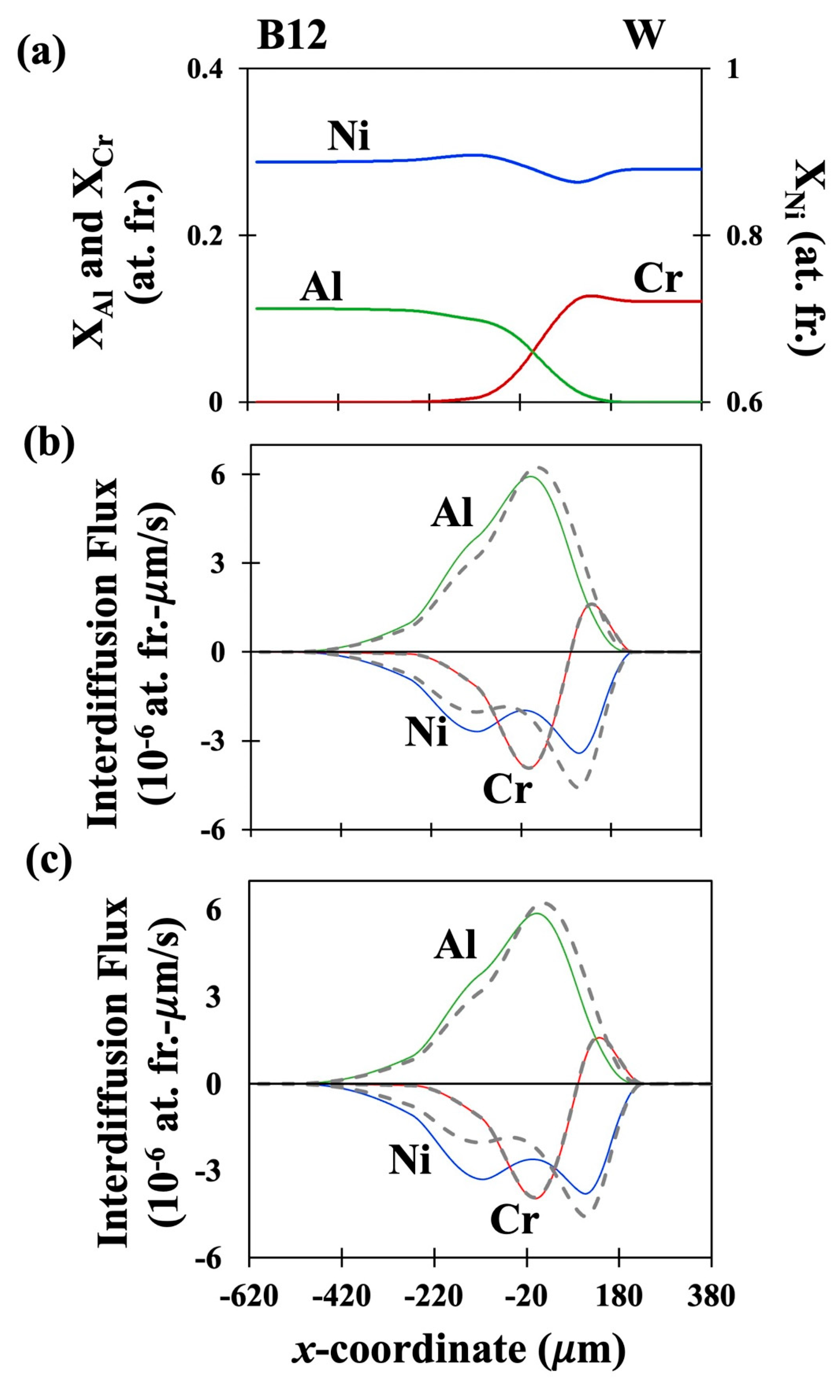
Figure 3.
(a) Fitted concentration profiles developed in Couple DC-3. (b) Interdiffusion flux profiles in as determined by newly developed Eq. (29) shown as solid lines. (c) Interdiffusion flux profiles in as determined by newly developed Eq. (32) shown as solid lines. In (b) and (c) the dashed lines show the fluxes determined by SF equation Eq. (38).
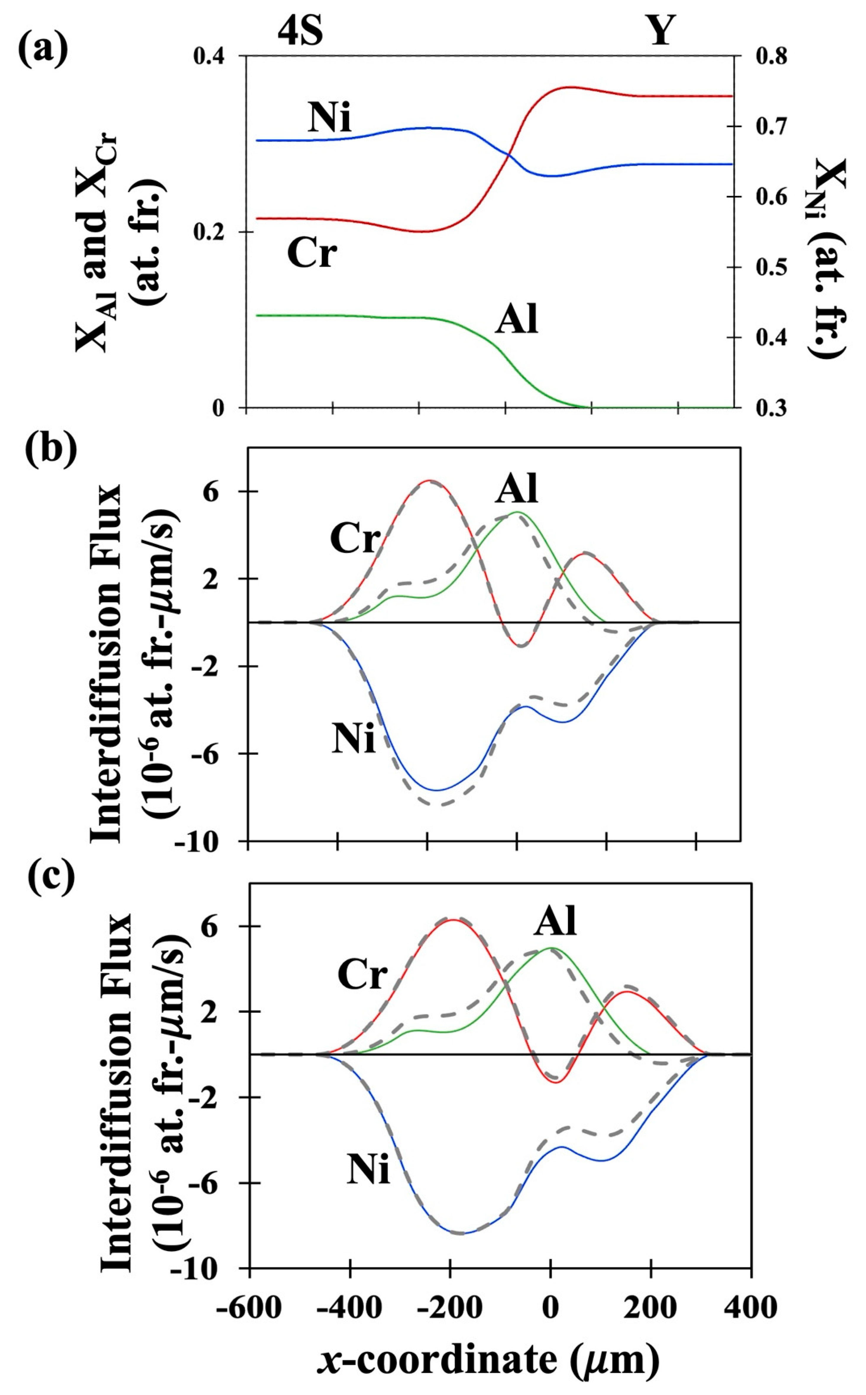
Figure 4.
(a) Variation of molar volume in the diffusion zone for three couples DC-1, DC-2 and DC-3. Solid lines are the actual molar volume and dashed lines are the ideal molar volume variation. (b) Percent variation of actual molar volume from ideality (c) Percent errors observed in interdiffusion flux if determined by SF Eq. (38) as against the correct and newly developed equation.

| Couple Designation | Terminal Alloys Composition (at%) as per [9] | Diffusion Annealing Temperature (°C) | Diffusion Annealing Time (hours) | ||||||
| Present Work | As per [9] | Left Terminal | Right Terminal | ||||||
| Ni | Cr | Al | Ni | Cr | Al | ||||
| DC-1 | 7S/1S | 86.9 | 7.7 | 5.4 | 57.9 | 35.9 | 6.2 | 1200 | 100 |
| DC-2 | B12/W | 88.8 | 0 | 11.2 | 88 | 12 | 0 | 1100 | 100 |
| DC-3 | 4S/Y | 70.1 | 18.6 | 11.3 | 64.8 | 35.2 | 0 | 1100 | 100 |
Disclaimer/Publisher’s Note: The statements, opinions and data contained in all publications are solely those of the individual author(s) and contributor(s) and not of MDPI and/or the editor(s). MDPI and/or the editor(s) disclaim responsibility for any injury to people or property resulting from any ideas, methods, instructions or products referred to in the content. |
© 2025 by the author. Licensee MDPI, Basel, Switzerland. This article is an open access article distributed under the terms and conditions of the Creative Commons Attribution (CC BY) license (https://creativecommons.org/licenses/by/4.0/).
Copyright: This open access article is published under a Creative Commons CC BY 4.0 license, which permit the free download, distribution, and reuse, provided that the author and preprint are cited in any reuse.


