
Submitted:
10 May 2025
Posted:
13 May 2025
You are already at the latest version
Abstract
This study examines the impact of Village Community Banks (VICOBA) on household welfare in Kilosa District, Tanzania. While VICOBA is recognized for improving livelihoods, concerns remain about its effectiveness on the welfare outcome of the participants. Using data from a randomly selected sample of 99 VICOBA members and 203 non-members, the research employed Propensity Score Matching (PSM) and Endogenous Switching Regression (ESR) methods to examine the impacts of VICOBA membership on welfare status of the households in Tanzania. Results showed a significant positive effect of VICOBA membership on household consumption, a key welfare indicator, with a 1% significance level. The ESR analysis confirmed these findings. The study concludes that VICOBA membership positively impacts household welfare and recommends that policymakers enhance operational systems and regulatory frameworks to better integrate these community banks into local development initiatives.
Keywords:
Village Community Banks
; household’s welfare
; Endogenous Switching Regression
; Propensity Score Matching
; Tanzania
1. Background
Globally, saving and credit institutions for the poor people have been there for several years, giving clients an alternative to get financial services as they were customarily ignored accessing such services by commercial banks (Ngalemwa, 2013). In fact, the fast growing need of financial services constrained by bureaucracy, remoteness and ignoring the poor who build a major group of world population alerts that something needed to be done about the suffering of the poor. With the difficulties of accessing financial services through financial institutions, microfinance models had developed to address the issue over that period since one among the common and well known microfinance institutions (The Bangladesh Grameen bank) was established by social entrepreneur, banker and economist Professor Muhammad Yunus in 1976, where VICOBA being one of them emerged. Though early idea was that of cooperative bank (i.e., Raiffeisen Bank) formed in Germany in 1864 so as to launch and spread the awareness of “self-help” in rural communities through offering savings and microcredit services, the Bangladesh experience is more relevant to VICOBA and operates worldwide as it is named in Asia as Self Help Groups (SHG) (Mashigo & Kabir, 2016; Ngalemwa, 2013).
In developing countries of Africa and Tanzania in particular there had been the same issue of minority exclusion in formal financial institutions. To address the challenge, microfinance model was adopted in early 1990s by CARE International starting in Niger and spread to other countries like Zimbabwe, Mozambique and Eritrea. Then it spread further to East African countries particularly in West Nile Uganda and in Zanzibar through CARE Tanzania in year 2000 (CEDIT, 2021). The model during its initial operation in these countries was given different names such asd OPHIVELLA in Mozambique, JENGA in Uganda and JOSACA in Zanzibar (Ngalemwa, 2013; Bakari et al., 2014). In Tanzania, VICOBA was first adopted from Niger, where the model was popularly known as “Mata Masu Dubara” (MMD) named in Hausa language which literally means “Women on the Move” as initiated by CARE Niger focusing on Women economic empowerment and poverty reduction. It was reformed by Social and Economic Development Initiatives of Tanzania (SEDIT) and registered as Village Community Banks, abbreviated as VICOBA (Bakari et al., 2014). According to the recent FinScope Surveys, there is significant share of Community Microfinance Groups led by VICOBA of about 12% in 2023 though dropped from 16% (2017) of the adults but absolutely greater from 12% of 2013 unlike formal saving groups (referring to SACCOs) whose share of the total adults is 1% in 2023 declined from 2% in 2017 and 3% of 2013 in Tanzania, and that 73% of those in community microfinance groups are found in members’ self-established saving groups (FinScope Tanzania, 2017, 2023). This means community self-established saving groups including VICOBA are significant in microfinance subsector hence financial sector in the country
Moreover, previous studies inadequately establish clear lines whether the celebrated impacts are really resulted from VICOBA program and not otherwise. Evidence from previous studies (for instance Kihongo, 2005; Ngalemwa, 2013; Ollotu, 2017; Massawe, 2020 and Dyanka, 2020) found that VICOBA has a positive relation to improvement of livelihood of low-income earners. But did not show the empirical analysis of VICOBA as a microfinance model on welfare status and how the impacts genuinely resulted from VICOBA. To assess its merit to propensity to save and invest; this study thought to employ impact evaluation where average treatment effects is assessed by establishing counterfactual to see actual changes brought by VICOBA in terms of welfare. Also, for the sake of the community to get out of viscous poverty there must be a seed for saving which is important for maintaining a level of investment, a key element of economic uplift. So, the research established a topic to deal with, that regardless of households struggle to put food on the plate and sustain today’s life, VICOBA should further be assessed as a bridge to get out of poverty, by looking at the practice of putting money aside to invest as the outcome of it. This study aims at filling the gap by analyzing the impact of VICOBA membership on the household welfare as measured by consumption expenditure while hypothesizing that consumption expenditures of the members’ households who are in VICOBA do not differ significantly from those who are non-members of VICOBA.
2. Methods and Material
2.1. Area of the Study
This study targeted to examine impact of VICOBA by taking a case from Kilosa district, one of the seven districts in Morogoro region, Tanzania located at latitude 60 50՛ 0՛՛S and longitude 360 59՛ 0՛՛E. The district has a total area of 12,394 square kilometers (17.5% of 70,624 km2 covering Morogoro region), out of that total land, 536,580 hectares are used for agriculture. The district is administratively divided into 7 Divisions, 40 Wards, 138 Villages and 814 Hamlets, having two township authorities of Kilosa and Mikumi (Kilosa District Council, 2020). The rationale of selecting Kilosa District lies on the fact that before the study the district had greater representation as it is one of the areas with concentrated VICOBA activities, having more than 200 registered groups with more than 4,300 members (Kilosa Distict Council, 2021).
2.2. Study Population and Sample
Referencing to the Population and Housing Census of 2012, Kilosa District had a population of 438,175 but 2018 population projection is 511,130, which is a 17% increase in population size over 6 years period (NBS, 2013; Kilosa District Council, 2020). This study had VICOBA participants as experiment group, from more than 200 registered groups with about 4,300 members (Kilosa Distict Council, 2021). But considering non-members as the reference population from which the program’s counterfactual will be drawn, observing that they both possess some shared characteristics and regarded as household in terms of unit of analysis. A total of 305 individuals were involved whose determination in this study was steered by a preset sample frame which based upon the population size, compositions, margin of error and number of other considerations. The sample size for this impact evaluation was estimated using the following formula;
where N = total sample size, = corresponding value for set level of confidence, P=proportion of event of interest for the study, E=margin of error and D=designed effect which is 1 for simple random sampling; this study used 95% level of confidence within 1% margin on error, so =1.96, P=0.008 i.e (4,300/511,130); E=0.01
To obtain sample of treatment (n1) and control (n2) for effective matching and maximizing power, most literatures suggest increasing the ration of control to treatment, so ratio of 1:2 was used to have n1= 102 and n2= 203. However, 302 successful observations were used as shown in Table 1, having 99 from experiment and 203 from control group after cleaning and dropping sample observations with some missing data.
2.3. Variables Definitions
This study uses a variety of variable in the estimation of the impact of Village Community Banks on household welfare. The variables have been selected based on the theories, empirical studies and common intuitions by the author. Table 2 presents the variables (outcome and covariates), their definition, measurements and expected signs.
2.4. Model Specification
To capture the impact of VICOBA consumption expenditure as dependent variables, we run the outcome on membership status including control variables such as dependents, training, education, employment, age, gender, married, working experience and microcredit. The general equation is,
Assuming that household is rational to membership, the utility gain from membership is conveyed as a function of observable characteristics (X) in a probit model as:
Such that
where is a binary variable; = 1 if household representative i is a VICOBA member and = 0 otherwise. is a cumulative standard normal distribution function, = vector of coefficients to be estimated and is a vector of household characteristics; and µi is a random error term assumed to be normally distributed.
Regression equation for outcome:
Yi =outcome variables consumption expenditure in different regressions for i, = membership dummy (it takes 1 if VICOBA member, 0 if not), =household characteristics, α is a constant, = effect of VICOBA (main parameter of interest), =coefficients to be estimated and is an error term.
2.5. Econometric Model Estimation
2.5.1. Propensity Score Matching (PSM)
Probit regression was used to obtain propensity scores on membership to enable matching the observations and then impact estimates by nearest neighborhood, radius matching and weighting as the joint consideration conveys a better way to assess robustness of the estimates in observational research. Conditional Independence assumption (CIA) or uncofoundedness is the central assumption of PSM to be met. This imply that, given a set of observable covariates which are not affected by treatment (membership), potential outcome of VICOBA non-members and members would have the same distribution, independent of membership. Also, common support or overlap condition to ensure that both treated and controls have common range of propensity scores was taken into account. According to Duvendack (2010) this ensures that individuals with the same values have positive probability of being members and non-members. However, in a particular case, it is satisfactory to assume that and such that the ATT be obtained as follows
where is the mean outcomes of treated individuals and is the calculation for the matches from control individuals (Duvendack, 2010). By weighing, the outcome regression equations are estimated by equation 3.2.
2.5.2. Endogenous Switching Regression (ESR)
The first step is decision to join VICOBA, which is a choice equation (equation 3.1), then it follows that the two regime outcome equations are:
where =household characteristics, and represent outcome variables for VICOBA members and non-members and are Error terms, and are the parameters to be estimated. Then; average treatment effect on treated (ATT) and average treatment effect on untreated (ATU) are given as;
where;
=expected outcome of members with membership of VICOBA (real)
= expected outcome of members if they were without membership of VICOBA (counterfactual)
= expected outcome of non-members if had membership of VICOBA (counterfactual)
= expected outcome of non-members without membership of VICOBA (real).
3. Results and Discussion
3.1. Descriptive Statistics
In general, 302 household representatives were observed with 99 from treatment group and 203 respondents from control group. Overall, 238 (81 from treatment and 157) who made 78.81 percent of the observations were female and remaining 21.19 percent were male, with an average of 43.95 years of age having a minimum of 18 years and maximum of 76 years. 75.83 percent of the sample were married and had an average of 3 dependents per household. The statistics imply that most households are coupled and sometimes headed by both young and old people, but on average, the population is active middle-aged which is economically productive.
The study also found that only 12.25 percent of the respondents had salaried employment (Table 3), meaning that the majority of the households depended on self-income generating activities led by 60.6 percent in crop cultivation and 17.88 percent in livestock keeping, with an average of about 20 and maximum of 55 years of working experience. These results are in line with available statistics that 79 percent of Kilosa district’s employment positions are within agriculture (NBS, 2013), meaning that people’s livelihood depend highly on agriculture and likely to have seasonal income fluctuations which affects individual household welfare status.
On average, respondents had an education level equivalent of standard III, with the highest level being a diploma level; meaning that the education level was generally low which also reflect the employment status of the households (Table 4). About 33.44 percent of all respondents hadn’t attained education at all while 47 percent had attended at least standard four to standard seven primary school education. The rest of about 20 percent had had a minimum of form two secondary education level and the maximum of ordinary diploma level.
The access to financial services is not quite easy since about 75.5 percent admitted that they (and other household members) neither own nor use bank accounts and rely on public transport with an average of more than 31 kilometers to reach any nearest bank. The 25.5 percent who have or use bank services is above average of 12.3 percent presented by 2017-18 household budget survey and only 16 percent shown in National Financial Inclusion Framework 2018-2022, but within a maximum average of 31.3 percent of households which have at least one person who operates a bank account (National Council for Financial Inclusion, 2018; NBS, 2019). On the other hand, only 17.88 percent declared to have got financial related training in the study area. These statistics indicate that many households incur substantive costs in terms of time and finances to access formal financial services and thus limited their usage of financial services and little is covered on financial literacy in the area. On VICOBA banking operations, members had an average share value contribution of TZS 6040, the minimum share value bought was TZS 1,000 and the maximum was TZS 15,000 per week per member. This means on average a person saves TZS 24,160 with VICOBA alternative per month. A mean value of loan provided was TZS 112,626.3 where maximum loan from VICOBA obtained was TZS. 600,000. Table A1 and Table A2 in appendices provides more of these descriptive and t-test means comparisons.
In terms of outcome variables, the descriptive as presented in Table 5 shows that on average monthly income spent on household consumption was used as an indicator of household welfare, where on average, household’s monthly income spent to finance the basic needs was TZS 133,698.7, where average for members was TZS 162030.3 and for non-members TZS 119881.8. Generally, a minimum monthly income spent was TZS 30,000 and a maximum of TZS 450,000, which is the daily average of TZS 4,456.62. Considering an average consumption per household per month in rural Tanzania mainland of TZS 361,956 (NBS, 2019), the result implies that on average, households in the study area are low income earners and thus limits their consumption opportunities, hence deprive their welfare attainments.
Table 6 indicate that a total of 203 non-members, which is 67.22 percent of the whole sample, and 99 VICOBA members, which makes 32.78 percent of the whole sample were observed. The PSM models matched the treated individuals with the untreated individuals based on the propensity score which was calculated based on the covariates thought to affect treatment status.
The individuals on treatment (VICOBA Members) were matched with corresponding untreated counterpart (non-members) which had a similar propensity score in a given range depending on the matching process. The propensity score in this study was estimated using a probit model as the results are shown in Table 4 with their marginal effects.
3.2. Econometric Results
In order to achieve the impact of VICOBA on household welfare (Consumption), the estimation procedures start with determining the probability to belong to VICOBA. This was done by estimating a probit model which is equation 3.1 estimated at 1%, 5% and 10% significant level. Results of estimation indicate that membership in VICOBA is significantly influenced by the marital status of the household head and the number of household’s dependents. The household dependency size has also a positive and significant effect on membership in VICOBA groups, where the household’s dependents increase has a higher probability (5%) of being members of VICOBA groups, this goes in contrast to estimation by Cintina & Love (2017), but concurs with the results by Ghalib et al (2011) who found that households with greater dependency ratio had a positive and statistically significant effect on the probability of joining microfinance programme. This reflects the fact that household members are in deprivation, inciting one of the members to join VICOBA may be with an expectation of gaining relief to smooth household consumption and accommodate the dependents. Other covariates which are age, gender, employment status, training and access to microcredit as well as working experience were found insignificant individually, partly contrary to Cintina & Love (2017) who found significant positive influence of age and gender (female) and negative influence of education on probability of joining microfinance programme. The other study found gender to have positive and other loans (microcredit) to have negative significant influence (Farida et al., 2016).

Table 7.
Probit estimation of membership in VICOBA.
| Variable | Coefficients | Marginal effects |
| Age | - 0.0037826 (0.0091624) |
-0.0013497 (0.00327) |
| Gender | -0.1758753 (0.1995059) |
-0.0611343 (0.06732) |
| Marital status | 0.4869904** (0.1896883) |
0.1614229** (0.05743) |
| Dependents | 0.1423543** (0.0580818) |
0.0507938** (0.02073) |
| Training | 0.1872583 (0.2027853) |
0.0685346 (0.07593) |
| Education | -0.0036312 (0.0099277) |
-0.0012957 (0.00354) |
| Employment | -0.0649559 (0.2686466) |
-0.0229002 (0.09355) |
| Microcredit | 0.1789046 (0.1577475) |
0.0640343 (0.05651) |
| Work Experience | -0.0068434 (0.0090912) |
-0.0024418 (0.00324) |
| Constant | -0.9467986** (0.4499891) |
|
| Log Likelihood | -182.54163 | |
| Prob > chi2 | 0.0399 | |
| Pseudo R2 | 0.0445 | |
| Number of obs. | 302 |
Standard errors in parentheses ***p<0.01, **p<0.05, *p<0.1. Source: Author’s computation of field data.
3.2.1. Testing the Assumption of the Model
For the PSM model to be sound, some assumptions or conditions of overlap or regions of common support, the balancing property and unconfoundness have to be met. Although these assumptions are not generally testable, the checking processes in the propensity score estimation procedure were done in this study to ensure the robustness of the estimated propensity scores. In the PSM procedure, the region of common support is selected by identifying the minimum and maximum propensity scores that are observed in both the treatment and control groups. The test for the balancing property is performed by comparing the means of propensity scores as well as covariates across both VICOBA members and non-members after matching algorithm is incorporated in the propensity score estimation procedure to ensure that the households are no longer different in covariates and the average propensity score between members and non-members and hence treatment effect on the treated can be estimated with no selection bias (Pantaleo & Chagama, 2018). Table 8 and Figure 2 and Figure 3 shows the test procedures.
Table 8.
Common support for propensity score matching.
| Treatment assignment | On support | Off support | Total |
|---|---|---|---|
| Untreated | 203 | 0 | 203 |
| Treated | 98 | 1 | 99 |
| Total | 301 | 1 | 302 |
Source: Author’s computation of field data.
Figure 1.
Kernel density of the estimated propensity score. Source: Author’s Computations based on filed data described in the text
Figure 1.
Kernel density of the estimated propensity score. Source: Author’s Computations based on filed data described in the text
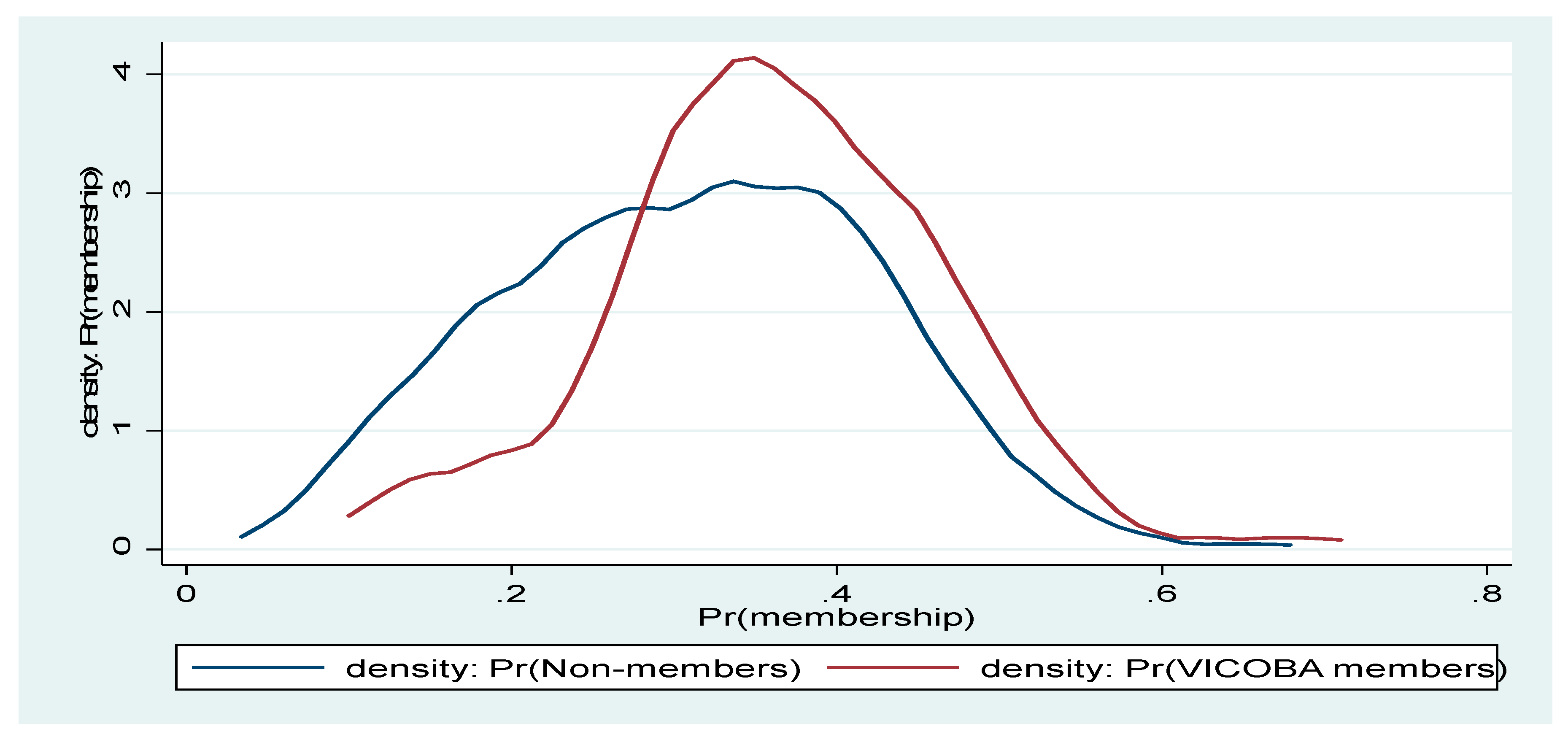
Figure 2.
Propensity score graph for both VICOBA members and Non-members. Source: Author’s Computations based on filed data.
Figure 2.
Propensity score graph for both VICOBA members and Non-members. Source: Author’s Computations based on filed data.
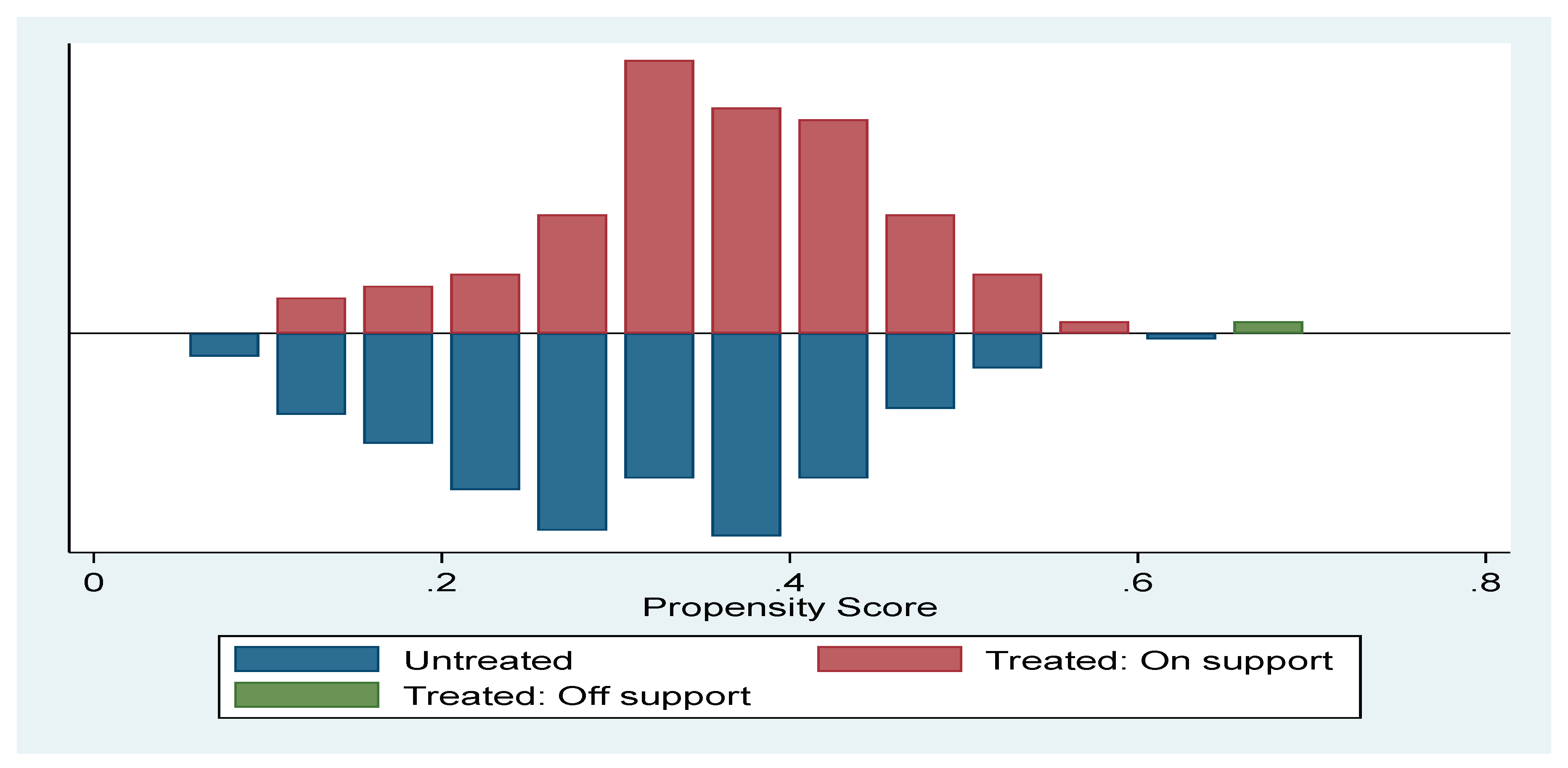
The two graphs (Figure 2 and Figure 3) show that there was overlapping of the propensity score between the treated and the control observations, suggesting that PSM estimation is possible as the two groups are comparable based on the described covariates. Further diagnostic approach of ensuring that the propensity scores can be used to assess the effect of treatment and addressing confounding is stratification. The observations were divided into strata/blocks based on the propensity score in a cross-tabulation of membership having both treatment and control observations by quintile. The results are presented in Table 9 showing that there are some treated and some untreated observations in every quintile of the propensity score, suggesting that it is possible to evaluate the effect of VICOBA membership in each block(quintile). Since the smaller the strata are, the better the balance of covariates and more confounding they remove, so it was then divided into deciles of the propensity score and it was still found to have both treated and untreated in each stratum as shown in appendix 5.
3.2.2. Estimating the Propensity Score Matching (PSM)
In order to have a potential counterfactual of the treated and then calculate ATT and test its significance using t statistical test we present the treatment effects estimated from the PSM models to match the treated and the control groups with similar observable. The validity and quality of this evaluations procedure depends on matching of the calculated propensity score between treated and the untreated observations (Austin, 2011). Therefore, several analyses were carried out to ensure that the propensity score satisfy the required property and hence the calculation of ATT is selection bias free. After ensuring that the conditions are met, impact was estimated using Nearest Neighbor caliper matching, then radius matching and linear regressions of weighted averages in common support as follows;
Nearest Neighborhood Matching (NNM) Estimations
The NNM method chooses the closest score from the covariate of the control group. The process is good for treatment group and control group that tend to be similar (Farida et al., 2016). In the matching process of PSM, the number of covariates that got paired in the matching or that got common support (Table 8) are 301 observations, of which 203 are for control group and 98 for the treatment group, only 1 treated observation was out of common support so not used in matching. Since the common support hypothesis is achieved with almost all units being reliable for matching, except one from treatment group, the NNM technique was possible and provides results similar to kernel with 0.05 bandwidth. The empirical estimations of the average treatment effect on the treated (ATT) within common support based on the equation 3.7 developed in the methodology section are as displayed in Table 10 with Nearest Neighbor Caliper matching within 0.05 caliper.
ATT is the difference in the outcome between the treatment and control groups, after controlling for covariates. It can only be estimated at the population or sample level and not at an individual level because it is the average effect of the treatment on the entire population, and not the effect of the treatment on any one individual.
Radius Matching Estimations:
Nearest-neighbor matches each treated unit with the control unit that has the most similar propensity score, therefore covering shortfalls of stratification matching which can lead to some treated units being discarded if there are no control units in their block. But NNM can lead to poor matches if the nearest neighbor has very different characteristics or propensity score from the treated unit. So, radius matching can address the limitations of stratification and nearest-neighbor matching. Radius matching matches each treated unit with control units that have propensity scores within a predefined radius of the treated unit's propensity score. This allows for more flexibility in matching treated units with control units, and it can lead to better covariate balance(Austin, 2011, 2014). Nevertheless, radius matching can also lead to some treated units not being matched if there are no control units within the radius; therefore, some treated units may be discarded from the analysis. So far, their joint consideration brings a better way to assess robustness of the estimates. In this case radius matching estimated the impacts with default radius size of 0.1 and the results are in Table 11.
3.2.3. Endogenous Switching Regression (ESR)
Estimation of impacts by most of non-experimental methods fails to capture observable and/or unobservable characteristics that affect choice and outcome variables, For example, Propensity Score Matching controls for observable covariates under the assumptions of overlapping or regions of common support, the balancing property and unconfoundness assumption (Austin, 2011). In comparison to, using regression models to analyze the impact using pooled samples of members and non-members might be improper since it gives the similar effect on both groups (Sileshi et al., 2019). So an estimation approach that overcomes these limitations is endogenous switching regression (ESR). According to Adlin et al., (2020) ESR models have a very strong exclusion restriction and the falsification test may not be sufficient to confirm identification, so results may be sensitive to selection of instrumental variables. Therefore, the use binary PSM is helpful to further robustness check of the results obtains from ESR as it adjusts for initial differences between treated and control groups by constructing a statistical comparison group using observed covariates on a probit model of selection decision.
The impact of VICOBA membership on household welfare under the ESR approach follows two stages. The first stage, decision to join VICOBA is estimated using a binary probit model as selection. After estimating a probit model which is for equation 3.1 (choice equation), the second step for ESR estimation to bear results is to estimate the two regime outcome equations which are equations 3.8 for treatment group and 3.9 for control group.
To ensure the validity of the instruments to be used before running ESR with full-information maximum likelihood, the probit model for the equation 3.1 was estimated and OLS regressions for outcome equations (3.8), and (3.9) separately and checked in which equation these variables were effectually significant considering only 1% and 5% significance level to check for endogeneity and satisfying exclusion restriction. Marital status and number of dependents were found strongly influencing selection equation. In consumption expenditure equation these instruments did not satisfy exclusion restriction as they were found to influence choice and outcome equations.
Nevertheless, the endogenous switching regression model is appropriate and valid method if the covariance and are significantly different from zero and/or if one of the estimates of correlation coefficients or is statistically significant, which show the existence of selection bias due to unobserved covariates (Hasebe, 2020; Christophe et al., 2020). So, for this case the method was valid to be used given the results in Table 12. The results derived by Endogenous Switching Regression model in estimating the impacts of VICOBA membership on household’s welfare (consumption expenditure) are shown in Table 12, where amounts are in TZS.
The average treatment effect on the treated (ATT) and the average treatment effect on untreated (ATU) were obtained by estimating equations 3.10 and 3.11 respectively for each outcome variable. The ATT provides average effects attributed by the programme on those involved in it (treated) as the difference between actual and its counterfactual, while ATU provides anticipated average effects of the programme on those who are not involved (control) as the difference between its counterfactual (what would have been the results for untreated if they were treated) and actual (as they are untreated) as shown in Table 13. The system of choice and two regime equations, that is equation (3.1), (3.8), and (3.9) are estimated simultaneously using full-information maximum likelihood method (Christophe et al., 2020).
The Impact of VICOBA Membership on Household Welfare
Impacts of VICOBA membership on household welfare was captured on monthly income spent on household basic consumption which was significant across both methods. Nearest neighbor matching results (Table 9) indicate monthly consumption expenditure difference after matching was TZS 27,183.67, where the average monthly income of treatment group was TZS 160,622.45 and the control groups was TZS 133,438.78, meaning that VICOBA members had higher expenditure than comparable non-members. These are supported by radius matching results (Table 10) with ATT of TZS 26624.49. ESR estimation shows results of the same direction though difference in magnitude, as Table 12 illustrate that ATT was TZS 126,787.7 where the average monthly expenditure of the treatment group was TZS 162,030.3 and its counterfactual had average of TZS. 35,242.64. The results are concurring with Chemin (2008) who found that joining microfinance had consumption smoothing effects in Bangladesh, similar to Ghalib et al., (2011) whose application of propensity score matching approach on evaluating the impact of microfinance on easing Poverty of rural households showed that microfinance significantly improve household income. Therefore supporting other descriptive and OLS results like those done by Ngalemwa (2013), Ollotu (2017) and Massawe (2020) in assessing VICOBA in Tanzania. The ATU presented in ESR results (Table 13) shows that VICOBA membership would have no significant impacts on income of non-members if they had received the treatment, since the observed difference of decrease by TZS 1125279 is not statistically significant.
In general, the results show that VICOBA affects households’ welfare through increased household incomes spent on basic consumptions, indicating that members increase their monthly income spent on household consumption which could be due to borrowing, profit from shares contribution or investment from the group, and hence are expected to have a better welfare compared to its counterfactual.
4. Conclusions
This study examined the impact of Village Community Banks (VICOBA) on households’ welfare status in Tanzania, citing Kilosa District as a case. An impact evaluation was done by employing Propensity Score Matching (PSM) and Endogenous Switching Regression (ESR) to reduce the effects of self-select bias due to both observable and unobservable covariates and ensure consistence of the results. In the first stage, the probit model indicates that marital status and number of household dependents are significantly associated with joining VICOBA, that married have a probability of joining VICOBA by 16 percent higher than those who are not married and an increase in the number of household dependents have higher probability of joining the program by 5 percent compared to their counterfactuals. The empirical results obtained from both estimation methods suggests rejecting the null hypotheses, revealing that VICOBA membership significantly contributes to improving welfare of the members of households. Although the magnitude of impacts is minimal considering level of investment, the positive results indicate evidence that if VICOBA is improved in practice, individual households’ welfare can be higher than the findings observed.
Policy Implication and Recommendations
Referring to findings of the study from literature to empirical results, it is vivid that financial institutions alone can’t achieve welfare of the people in improving economic growth as well as poverty reduction as the country’s and global goal. Microfinance subsector’s broader change is required towards demand and access-based models that affect the majority in time, of which VICOBA is the lead community microfinance model to cover financial inclusion gap. It also implies that there is operational gap which means Government and development partners should pay more attention on integrating VICOBA not just improved financial practices but also the business development services to advance their occupational practices and other income generating activities that will help to reduce vulnerability of unbanked population to external shocks. There is a need to add effort on technical, expertise and financial assistance through integrating VICOBA activities in Local Government Authorities’ development plans, this can provide easy and effective link between government’s credit schemes and unbanked low-income segments of the population because the groups are clear and ease to manage (self-managed) and run financial services to members with low costs.
Appendix A
Table A1.
Descriptive statistics of household covariates and outcome variables.
| Characteristics | Description | Members Nt=99 |
Non-members Nc=203 |
Total sample N=302 |
|||
|---|---|---|---|---|---|---|---|
| Mean | SD | Mean | SD | Mean | SD | ||
| Age | Age of head in years | 43.2 | 11.3 | 44.3 | 11.5 | 43.9 | 11.4 |
| Gender | Dummy of gender (1=male) | 0.18 | .39 | 0.23 | 0.42 | 0.21 | 0.41 |
| Marital status | Dummy of marriage (1=married) | 0.85*** | 0.36 | 0.714 | 0.453 | 0.758 | 0.429 |
| Dependents | Number of dependents | 2.98 ** | 1.355 | 2.576 | 1.349 | 2.709 | 1.362 |
| Training | Dummy for financial training (1=Yes) | 0.212 | 0.411 | 0.163 | 0.369 | 0.179 | 0.384 |
| Education | Level of education in number of year | 12.485 | 9.571 | 12.897 | 9.679 | 12.762 | 9.629 |
| Employment | Dummy for employment (1=Salaried employment) | 0.121 | 0.328 | 0.123 | 0.329 | 0.123 | 0.328 |
| Microcredit | Dummy for obtaining microcredit (1=Yes) | 0.475 | 0.502 | 0.438 | 0.497 | 0.45 | 0.498 |
| Experience | Working experience in years | 19.162 | 11.896 | 20.379 | 11.896 | 19.98 | 11.89 |
| Outcome variables | |||||||
| Cons. expenditure | Monthly income in consumption expenditure (in TZS) | 162030.3*** | 92645.3 | 119881.8 | 65175.21 | 133698.7 | 77704.3 |
***Significant 1%, **significant 5% and *significant 10%.
Table A2.
T-test mean comparison between VICOBA members and non-members.
| Non-members Nc=203 |
Members Nt=99 |
T-test N=302 |
||
| Mean | Mean | Mean difference | t-statistics | |
| Characteristics | ||||
| Age | 44.31 | 43.222 | 1.088 | 0.78 |
| Gender | 0.227 | 0.182 | 0.045 | 0.89 |
| Marital status | 0.714 | 0.848 | 0.134 | -2.58*** |
| Dependents | 2.576 | 2.979 | 0.403 | -2.44** |
| Training | 0.163 | 0.212 | 0.049 | -1.05 |
| Education | 12.897 | 12.485 | 0.412 | 0.35 |
| Employment | 0.123 | 0.121 | 0.002 | 0.05 |
| Microcredit | 0.438 | 0.475 | 0.037 | -0.59 |
| Experience | 20.379 | 19.162 | 1.217 | 0.83 |
|
Easy of access to bank services | ||||
| Use/ownership of bank account | 0.227 | 0.283 | 0.056 | -1.06 |
| Distance to nearest Bank | 31.502 | 30.808 | 0.694 | 0.26 |
|
Outcome variables | ||||
| Saving | 17965.52 | 29979.8 | 12014.28 | -2.93*** |
| Investment | 117576.4 | 355000 | 237423.6 | -3.98*** |
| Cons. expenditure | 119881.8 | 162030.3 | 42148.5 | -4.57*** |
***Significant 1%, **significant 5% and *significant 10% for mean difference.
Table A3.
Summary of VICOBA banking services (share and loans).
| Variable | Observations | Mean | Std. Dev. | Min | Max |
| VICOBA share | 99 | 6040.404 | 3559.75 | 1000 | 15000 |
| VICOBA loan | 99 | 112626.3 | 161210.9 | 0.000 | 600000 |
Mean, Minimum and Maximum values in TZS.
References
- Austin, P. C. (2011). An introduction to propensity score methods for reducing the effects of confounding in observational studies. Multivariate Behavioral Research, 46(3), 399–424. [CrossRef]
- Austin, P. C. (2014). A Comparison of 12 Algorithms for Matching on the Propensity Score, (September 2013). [CrossRef]
- Bakari, V., Magesa, R., & Akidda, S. (2014). Mushrooming Village Community Banks in Tanzania: Is it really making a difference? International Journal of Innovation and Scientific Research. ISSN 2351-8014, Vol. 6 No. 2, PP. 127-135.
- Cintina, I., & Love, I. (2017). Re-Evaluating Microfinance Evidence from Propensity Score Matching, (April). Policy Research Working Paper 8028.
- Duvendack, M. (2010). Smoke and Mirrors: Evidence from Microfinance Impact Evaluations in India and Bangladesh. 1–271.
- Dyanka, E.W (2020). The Role of Village Community Banks (VICOBA) on Economic Empowerment to Women Smallholder Farmers in Kilosa District, Tanzania. 2507(February), 1–9.
- Farida, F., Siregar, H., & Nuryartono, N. (2016). An Impact Estimator Using Propensity Score Matching: People’s Business Credit Program to Micro Entrepreneurs in Indonesia, 20(4), 599–615.
- FinScope Tanzani (2017). “SACCOs and Savings Groups: Who do they serve and what do members utilize them for?” Financial Sector Deepening Trust, Dar es salaam, Tanzania.
- FinScope Tanzania (2023). Insights that Drive Innovation.
- Ghalib, A. K., Malki, I., & Imai, K. S. (2011). The Impact of Microfinance and its Role in Easing Poverty of Rural Households: Estimations from Pakistan. Discussion Paper Series-Kobe University, 1–33.
- Kihongo, R. M. (2005). Impact Assessment of Village Communitity Bank (VICOBA), a Microfinance Project at Ukonga Mazizini. 81pp.
- Kilosa District Council (2020). Kilosa District Investment Profile Opportunities and Promotion Strategies; April 2020. Accessed at http://kilosadc.go.tz on 20 November, 2021.
- Mashigo, P., & Kabir, H. (2016). Village banks: A financial strategy for developing the South African poor households. Banks and Bank Systems, 11(2), 8–13. [CrossRef]
- Massawe, J. J. (2020). The Role of VICOBA in Improving Livelihood Among Low Income. National Council for Financial Inclusion. (2018). National financial inclusion framework, 2018 - 2022.
- NBS. (2013). 2012 Population and Housing Census: Population Distribution by Administrative Areas. Dar Es Salaam, Tanzania.
- NBS. (2019). The 2017-18 Household Budget Survey: Key Indicators Report. Dodoma, Tanzania.
- Ngalemwa, D. M. (2013). The Contribution of Village Community Banks to Income Poverty Alleviation in Rufiji Delta. Sokoine University of Agriculture, Tanzania.
- Ollotu, A. A. (2017). Contribution of Village Community Banks (VICOBA) to economic development of women in Tanzania: a case of Dodoma. http://repository.udom.ac.tz/handle/20.500.12661/305.
- Pantaleo, I. M., & Chagama, A. M. (2018). Impact of Microfinance Institutions on Household Welfare in Tanzania: Propensity Score Matching Approach. The African Review, 45(2), 168–203.
- SEDIT (2021). Social and Economic Development Initiatives of Tanzania - Home (seditvicoba.or.tz) cited on 24 November 2021 at 10.55am.
- Sileshi, M., Kadigi, R., Mutabazi, K., & Sieber, S. (2019). Impact of Soil and Water Conservation Practices on Household Vulnerability to Food Insecurity in Eastern Ethiopia: Endogenous Switching Regression and Propensity Score Matching Approach. [CrossRef]
- Hasebe, T. (2020). Endogenous Switching Regression model and treatment effects of count-data outcome. The Stata Journal, 627–646. [CrossRef]
- Adjin, K. Christophe; Goundan, Anatole; Henning, Christian H. C. A.; Sarr, Saer (2020) : Estimating the impact of agricultural cooperatives in Senegal: Propensity score matching and endogenous switching regression analysis, Working Papers of Agricultural Policy, No. WP2020-10, Kiel University, Department of Agricultural Economics, Chair of Agricultural Policy, Kiel, https://nbn-resolving.de/urn:nbn:de:gbv:8:3-2021-00299-3.
Table 1.
Sample distribution by locality.
|
Locality/ward |
Group |
Total sample |
Percent |
|
| Control | Treatment | |||
| Magomeni | 18 | 19 | 27 | 8.94 |
| Rudewa | 20 | 10 | 30 | 9.93 |
| Madoto | 22 | 19 | 41 | 13.58 |
| Mabwerebwere | 26 | 9 | 35 | 11.59 |
| Kimamba B | 14 | 14 | 28 | 9.27 |
| Mvumi | 43 | 8 | 51 | 16.89 |
| Dumila | 37 | 17 | 54 | 17.88 |
| Msowero | 23 | 13 | 36 | 11.92 |
| Total | 203 | 99 | 302 | 100.00 |
Source: Author’s computation of field data.
Table 2.
Variables definition, measurements and their expected signs.
| Type | Name | Definition | Measurement | Exp. sign |
| Outcome variable | Consumption expenditure | Household income spent on potential consumption | TZS | |
| Independent variables | Membership | If VICOBA member or not | Dummy, 0-1 | |
| Education | Years of schooling | Numbers | + | |
| Dependents | Number of dependents | Numbers | - /+ | |
| Age | Respondent’s age | years | +/- | |
| Gender | If female or male | Dummy, 0-1 | +/- | |
| Training | Financial trainings | Dummy, 0-1 | + | |
| Married | If married or otherwise | Dummy, 0-1 | + | |
| Employment | If salaried employment or not | Dummy, 0-1 | + | |
| Experience | Years of working | Numbers | + | |
| Microcredit | If received Microloans out of VICOBA or not | Dummy, 0-1 | + |
Source: Author based on literature.
Table 3.
Employment status of the respondents.
| Employment category | VICOBA Membership | Total | ||||
| Non-members | Members | |||||
| n | % | n | % | n | % | |
| Crop Farming | 131 | 64.53 | 52 | 52.53 | 183 | 60.60 |
| Livestock keeping | 31 | 15.27 | 23 | 23.23 | 54 | 17.88 |
| Salaried employment-in government | 19 | 9.36 | 6 | 6.06 | 25 | 8.28 |
| Salaried employment-private sector | 6 | 2.96 | 6 | 6.06 | 12 | 3.97 |
| Self-employed | 11 | 5.42 | 9 | 9.09 | 20 | 6.62 |
| Casual labourer | 5 | 2.46 | 3 | 3.03 | 8 | 2.65 |
| Total | 203 | 100 | 99 | 100 | 302 | 100 |
Source: Author’s Computations of field data.
Table 4.
Educational status of the respondents.
| Education level | VICOBA Membership | Total | ||||
| Non-members | Members | |||||
| n | % | n | % | n | % | |
| No education | 67 | 33.00 | 34 | 34.34 | 101 | 33.44 |
| Standard four | 5 | 2.46 | 2 | 2.02 | 7 | 2.32 |
| Standard seven | 90 | 44.33 | 45 | 45.45 | 135 | 44.70 |
| Form two | 9 | 4.43 | 2 | 2.02 | 11 | 3.64 |
| Form three | 0 | 0.00 | 1 | 1.01 | 1 | 0.33 |
| Form four | 16 | 7.88 | 8 | 8.08 | 24 | 7.95 |
| Form four (+training course) | 12 | 5.91 | 6 | 6.06 | 18 | 5.96 |
| Ordinary diploma | 4 | 1.97 | 1 | 1.01 | 5 | 1.66 |
| Total | 203 | 100 | 99 | 100 | 302 | 100 |
Source: Author’s Computations of field data.
Table 5.
Summary statistics of outcome variables (monthly consumption expenditure).
| Consumption expenditure | ||
|---|---|---|
| Percentile | Smallest | |
| 1% | 30000 | 30000 |
| 5% | 45000 | 30000 |
| 10% | 60000 | 30000 |
| 25% | 90000 | 30000 |
| 50% | 120000 | |
| Largest | ||
| 75% | 150000 | 450000 |
| 90% | 240000 | 450000 |
| 95% | 300000 | 450000 |
| 99% | 450000 | 450000 |
| Obs. | 302 | |
| Sum of Wgt. | 302 | |
| Mean | 133698.7 | |
| Std. Dev. | 77704.3 | |
Source: Author’s Computations of field data.
Table 6.
Summary of Treatment Status.
| VICOBA membership | Frequency | Percent | Cum. percent |
|---|---|---|---|
| Non-members | 203 | 67.22 | 67.22 |
| Members | 99 | 32.78 | 100 |
| Total | 302 | 100 |
Source: Author’s computation of field data.
Table 9.
Blocks of propensity score for treatment.
| Quintile of pscore | Membership | Total | |
|---|---|---|---|
| Non-members | Members | ||
| 1 | 54 88.52 |
7 11.48 |
61 100.00 |
| 2 | 45 75.00 |
15 25.00 |
60 100.00 |
| 3 | 32 51.61 |
30 48.39 |
62 100.00 |
| 4 | 38 64.41 |
21 35.59 |
59 100.00 |
| 5 | 34 56.67 |
26 43.33 |
60 100.00 |
| Total |
203 67.22 |
99 32.78 |
302 100.00 |
Numbers in rows are in frequency and percentage. Source: Author’s computations based on field data.
Table 10.
PSM impact estimator using Nearest Neighbor Matching.
| Variable | Sample | Treated | Controls | Difference | S.E. | T-stat |
|---|---|---|---|---|---|---|
| Consumption expenditure | Unmatched | 162030.30 | 119881.77 | 42148.53 | 9225.72 | 4.57 |
| ATT | 160622.45 | 133438.78 | 27183.67 | 13238.14 | 2.05** | |
| Number of obs | = 302 | |||||
| LR chi2(9) | = 17.02 | |||||
| Prob > chi2 | = 0.0484 | |||||
| Pseudo R2 | =0.0445 | |||||
| Log likelihood | -82.54163 | |||||
***significant 1%, **significant 5% and *significant 10%. Unmatched=before matching, ATT=Average treatment on the treated Source: Author’s computation of field data.
Table 11.
PSM impact estimator using Radius Matching.
| Variable | Sample | Treated | Controls | Difference | S.E. | T-stat |
|---|---|---|---|---|---|---|
| Consumption expenditure | ATT | 160622.45 | 133997.96 | 26624.49 | 11639.74 | 2.29** |
| Number of obs | = 302 | |||||
| LR chi2(9) | = 17.02 | |||||
| Prob > chi2 | = 0.0484 | |||||
| Pseudo R2 | =0.0445 | |||||
| Log likelihood | -82.54163 | |||||
***significant 1%, **significant 5% and *significant 10%. Source: Author’s computation of field data.
Table 12.
ESR Regression of Consumption expenditure (Full Information Maximum Likelihood).
| Variable | Consumption expenditure | ||
| Selection Equation | Members | Non-Members | |
| Constant | -0.9468 (0.00003)** | -634052 (341564.8)* | 132498.1 |
| Age | -0.0038 (0.0025) |
-5038.499 (6339.976) | -1698.267 (522.0136) *** |
| Gender | -0.1759 (0.1697) |
-77502.38 (147830.4) | -6015.495 (35569.7) |
| Marital status | 0.487 (0.00003)** |
236546.5 (165425.4) | 74357.94 |
| Dependents | 0.1424 (0.000006)** | 82583.39 (45303.07)* | 37695.41 |
| Experience | -0.0068 (0.000006) |
-1031.306 (6113.879) | 461.6654 |
| Education level | -0.0036 (0.0073) |
-2199.628 (6807.299) | -6.642257 (1532.195) |
| Employment | -0.065 (0.2408) |
-9243.064 (193235.8) | 21395.46 (50478.54) |
| Financial training | 0.1873 (0.1915) |
113010.3 (143808.1) | 19008.09 (40145.44) |
| Microcredit | 0.1789 (0.1422) |
44692.56 (127297.3) |
13882.36 (29805.9) |
| σ0 | 209648.8 | ||
| σ1 | 556431.7 | ||
| ρ0 | -1.0000** | ||
| ρ1 | 1.0000 | ||
| Log likelihood | -77893.73 | ||
| Number of obs | 302 | ||
***p<0.01, **p<0.05 and * p<0.1. Standard errors in parentheses. Source: Author’s computation of field data.
Table 13.
Average treatment effects using Endogenous Switching Regression.
| Outcome variable | Treatment effect type | Decision stage | Treatment effect | |
| To be a member | Not be a member | |||
| Consumption expenditure | ATT | 162030.3 | 35242.64 | 126787.7*** |
| ATU | -790665.3 | 334613.8 | -1125279 | |
***Significant 1%, **significant 5% and *significant 10%. Source: Author’s computation of field data,.
Disclaimer/Publisher’s Note: The statements, opinions and data contained in all publications are solely those of the individual author(s) and contributor(s) and not of MDPI and/or the editor(s). MDPI and/or the editor(s) disclaim responsibility for any injury to people or property resulting from any ideas, methods, instructions or products referred to in the content. |
© 2025 by the authors. Licensee MDPI, Basel, Switzerland. This article is an open access article distributed under the terms and conditions of the Creative Commons Attribution (CC BY) license (http://creativecommons.org/licenses/by/4.0/).
Copyright: This open access article is published under a Creative Commons CC BY 4.0 license, which permit the free download, distribution, and reuse, provided that the author and preprint are cited in any reuse.


