Submitted:
12 May 2025
Posted:
13 May 2025
You are already at the latest version
Abstract
The SPICAV IR spectrometer on board the Venus Express mission measured spectra of the 1.1- and 1.18-μm atmospheric transparency windows at the Venus night side. The H2O volume mixing ratio in the deep Venus atmosphere at about 10-16 km has been retrieved for the entire SPICAV IR dataset using a radiative transfer model with multiple scattering. One of the challenges in modeling Venus’ night-side thermal emission in transparency windows is the deviation of the far wings of H2O and CO2 absorption lines from the Lorentz profile. Depending on the chosen approach to calculate the H2O absorption, the volume mixing ratio is: 27.1±1.1 ppmv for the Voigt profile, 26.9 ± 1.0 for the semi-empirical MT_CKD water vapor continuum model, 23.6±1.0 ppmv for the super-Lorentzian line profile. The zonal mean of the water vapor VMR do not vary significantly from 60°S to 70°N. Observations of polar latitudes are characterized by the increased noise level and might show a slight H2O mixing ratio decrease of 2 ppmv. No prominent long-term change on the time scale of 8 years nor local time variations of water vapor were detected.
Keywords:
Venus atmosphere
; infrared spectroscopy
; acousto-optical tunable filter spectrometer
1. Introduction
Venus has a dense CO2-atmosphere with a very low water content. Whether liquid water has ever existed on Venus remains unresolved. The presence of significant amounts of water in some form in the past is supported by the anomalous isotopic ratio of HDO to H2O. In the lower atmosphere of Venus, the HDO/H2O ratio is approximately 150 times higher than on Earth [1], and above the clouds it has been measured to be 240±25 terrestrial values [2]. The loss of water from Venus can be attributed to the dissociation of its molecules into oxygen and hydrogen. In the absence of a magnetic field on Venus, the loss of light hydrogen molecules by the atmosphere is significant [3]. Water vapor contained in the lower atmosphere plays a crucial role in the formation of sulfuric acid (H2SO4) clouds, which enshroud the planet by a layer extending from 47 to 70 km. A potential supply of water vapor is volcanic degassing [4]. Thus, study of the abundance and distribution of water vapor in the lower atmosphere allows us to gain a comprehensive understanding of the chemistry and evolution of Venus.
The contribution of water vapor to the present greenhouse effect is relatively minor on Venus, which is the opposite of what occurs on the Earth. However, H2O absorption regulates the transmission of several infrared (IR) transparency windows of the Venus atmosphere. The atmospheric windows are narrow spectral intervals between strong CO2 absorption bands and were discovered by Allen and Crawford in 1983 [5]. Thermal radiation escaping to outer space in transparency windows provides one of the most effective remote sensing tools to investigate composition of the Venus near-surface atmosphere. Spectral windows at 1.1, 1.18, 1.74 and 2.3 μm are overlapped by the H2O absorption bands and correspond to thermal emission originating at different altitudes in the Venus atmosphere. The 1.1- and 1.18-μm windows allow sensing the Venus surface and the altitudes of 0-15 km. Thermal emission in the 1.74-µm and 2.3-μm windows is formed at 15-30 km and 30-45 km correspondingly [6].
The water vapor is well mixed below the clouds. Its volume mixing ratio (VMR) in the Venus lower atmosphere was obtained close to 30 ppmv (parts per million) without vertical evolution in remote observations. Spectra obtained during descent of Venera 13 and 14 landers proposed two H2O profiles: (1) a uniform distribution with VMR of 30 ppmv, (2) a decrease from 30 ppmv at the lower cloud boundary down to 20 ppm at 10-20 km and then an increase up to 50-70 ppmv below 5 km [7]. It was not possible to distinguish between the two conclusions due to experimental uncertainties [7]. Sensitivity to H2O absorption at altitudes of 0-5 km is low for observations in transparency windows [8,9], and it is discussed in Section 3. Table 1 presents the summary of the H2O observations in the transparency windows. Spatial variations of water vapor have not been observed in the 1.18 µm [10,11] and 1.74 µm [11] windows. At higher altitudes, spatial inhomogeneity of water vapor was detected [11,12], and an anti-correlation between H2O and cloud opacity was suggested [12].
We present the first complete analysis of observations in the 1.1 and 1.18 µm transparency windows by the SPICAV (SPectroscopy for the Investigation of the Characteristics of the Atmosphere of Venus) spectrometer on board Venus Express [27]. The abundance of water vapor in the deep atmosphere of Venus was studied over a period of 8 years, updating and extending the results of previous studies [8,9]. The data coverage corresponds almost to the whole night hemisphere and is described in Section 2. The developed forward radiative transfer model and retrieval algorithm are presented in Section 3. The retrieved water vapor abundance is reported in Section 4 and discussed in Section 5. Conclusions are presented in Section 6.
2. Observational Dataset
The IR channel of the SPICAV spectrometer operated on board the Venus Express spacecraft from April 2006 to December 2014 [27,28]. The instrument was based on the acousto-optical tunable filter (AOTF) technology, and the spectrum was recorded sequentially by tuning the AOTF to a specific wavelength. The full spectral range of the instrument was 0.65-1.7 μm with the ability to limit a spectral range and to choose sampling. The filter split the incoming light into two beams with orthogonal polarizations, which were focused onto two Si-InGaAs photodiode detectors. The silicon and InGaAs sensors were sensitive to radiation in the spectral ranges of 0.65-1.05 μm and 1.05-1.7 μm. The spectral resolution within these ranges was 7.8 cm-1 and 5.2 cm-1, respectively. The detectors could be cooled by integrated Peltier elements to increase the signal-to-noise ratio. Venus transparency windows required a long exposure time, which was 44.8 and 89.6 ms per spectral point. The signal-to-noise ratio (SNR) was 50 for 89.6 ms exposure time and cooled detectors, and the noise doubled without cooling [27]. For each observation, the signal noise was determined as the standard deviation of the radiance at 1.21-1.24 μm, where the atmosphere is opaque. When this spectral interval was not observed to reduce the duration of a measurement, spectrum uncertainties were estimated based on the SNR proportionally to the square root of the exposure time. The wavelength was assigned to the spectral point based on the AOTF parameters, and the calibration uncertainty is less than 0.2 nm. Radiance calibration accuracy was estimated to be better than 20%. The details on the SPICAV IR calibration can be found in Ref. [27].
The field of view (FOV) of the SPICAV spectrometer was circular with an angular size of 2°. The Venus Express orbit was elongated with a pericenter near the North Pole, and the spacecraft altitude varied from 250 km to 66000 km. Thus, the SPICAV footprint diameter varied from 9 km to 2300 km from northern to southern latitudes, and the observations of the Southern Hemisphere had lower spatial resolution. The spatial coverage, with an indication of the SPICAV footprint at the surface, is shown in Figure 1.
The instrument could observe the Venus transparency windows at 1.0, 1.1, 1.18, 1.28 and 1.31 μm. Due to the long integration time of one spectral point, the measurements of the transparency windows are spatially separated in the northern hemisphere. To minimize the influence of spatial shifts in the data analysis, we limit the analyzed spectral range to 1.06-1.21 μm, covering the 1.1 and 1.18 μm windows to study the water vapor content in the lower atmosphere of Venus.
Figure 1.
Spatial distribution of the 1.1- and 1.18-µm transparency window observations analyzed in this study. (A) Color indicates the orbit number. (B) Color codes for the diameter of the instrument’s footprint in kilometers. The data is overlaid with a topographic map from the Magellan space mission [29,30].
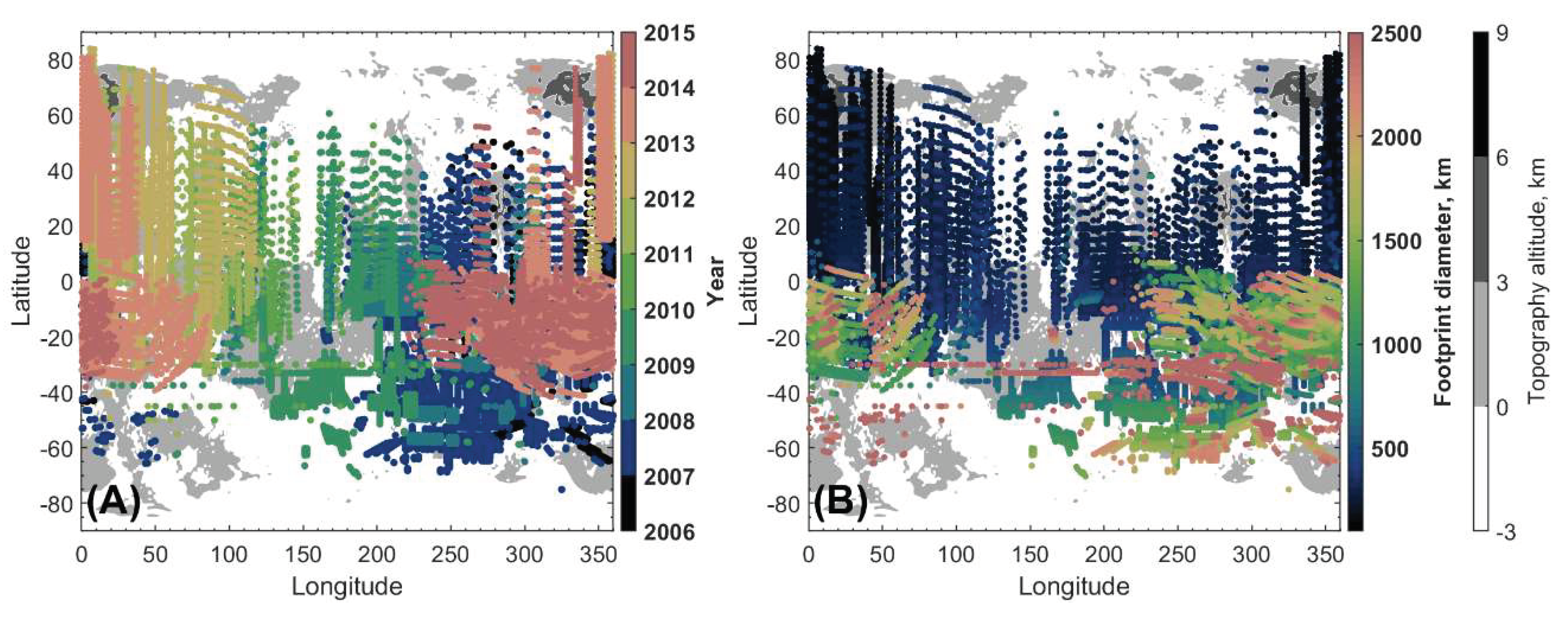
When measurements are made with large footprints or close to the terminator, the spectra may contain a fraction of scattered solar light that appears as a continuous background. This contribution was removed from the data by linear interpolation based on the 1.21-1.24 μm interval. In the case of strong contamination, linear interpolation is inefficient and the spectrum was not considered in the analysis. The selected observations overlap the Venus solar local times from 18:20 to 5:40. During 8 years of the Venus Express mission, the latitude range from 75°S to 84°N and almost the entire longitude range was observed. Due to Venus’ slow rotation, longitude coverage depends on the year of the space mission (Figure 1). The total dataset consists of more than 2600 observation sessions, corresponding to approximately 27000 spectra.
3. Methods
3.1. Radiative Transfer Model
A radiative transfer model including multiple scattering is developed to synthesize transparency window spectra. The radiative transfer equation is solved using the discrete ordinate method in a pseudo-spherical geometry implemented in the DISORT4 program package [31,32]. Emission angles of 60-75° constitute 1% of the analyzed dataset where the pseudo-spherical approximation is necessary. Sixteen streams were used.
The atmospheric structure is set by vertical profiles of temperature and optical properties (optical depth of computational layers, single scattering albedo and Legendre series expansion of the scattering phase function). The upper boundary is set at 100 km above the reference sphere, and the atmosphere is divided into discrete homogeneous layers of 1 km. For altitude profiles of temperature, pressure, and density, the Venus International Reference Atmosphere (VIRA) [33] is used, which is based on the descend probe measurements. The surface temperature is set equal to the atmospheric temperature at the altitude of local elevation, which is calculated from Magellan data [29,30] as an average within the SPICAV IR footprint.
Clouds are modeled according to a three-layer cloud model based on the Ref. [34], where the aerosol particles are represented by four modes: 1, 2, 2’ and 3. Each mode follows a log-normal size distribution with the effective radius of 0.3, 1.0, 1.4, 3.65 μm and the dimensionless dispersion of 1.56, 1.29, 1.23, 1.28, respectively [6,34]. The real part of the refractive index and its dependence on the wavelength are very close for different acidity of H2SO4-solution in the spectral range 1.06-1.21 μm, and the concentration in the cloud model is fixed to 75%. Wavelength-dependent microphysical parameters, as aerosol extinction, single-scattering albedo and the Legendre expansion coefficients of the scattering phase function, are computed using the Mie theory [35] for each mode.
The radiance of the 1.1- and 1.18-μm transparency windows forms at 0-15 km (Figure 2A). The deep atmosphere has a large thermal inertia preventing diurnal variations of temperature. Based on the multispectral images by the Near-Infrared Mapping Spectrometer on board the Galileo spacecraft, horizontal temperature variations were constrained to ±2 K on the Venus night side [36]. Surface emissivity also affects radiance in the spectral windows. Decreasing the emissivity from 0.95 to 0.4 results in 16% and 15% attenuation in 1.1- and 1.18-μm transparency windows, respectively (Figure 2C). Absolute emissivity values of the Venus surface in the near-infrared (NIR) range are poorly known, and it is difficult to retrieve them [37]. Nevertheless, the emissivity variation over the surface was observed and linked to the different geological areas: tesserae, basaltic plains or recent lava flows [38]. A general decrease in emissivity was also associated with a higher elevation area [36,38]. In the current analysis surface emissivity was set to 0.95, and the sensitivity of the retrieval water vapor volume mixing ratio to this parameter is discussed in Section 4.
The absorption of CO2, H2O and HDO is included in the model. The CO2 mixing ratio is set to 0.965. H2O and HDO are assumed to be uniformly mixed under clouds. The radiance of the 1.1- and 1.18-μm transparency windows is sensitive to variations in the H2O volume mixing ratio (VMR) in altitude range of 4-22 km with peak sensitivity at 10 km. The core of the H2O absorption band is between two spectral windows at 1.12-1.16 μm, and radiance sensitivity to the H2O abundance extends from 7 to 30 km with peak at 16 km. The sensitivity is evaluated as the radiance change at each wavelength induced by water vapor VMR increase of 1 ppmv (Figure 2B). The limits of model sensitivity to H2O VMR change are defined as a full width at half maximum of the obtained radiance change profile. Consequently, the spectrum exhibits minimal sensitivity to a potential gradient within the range of 0-5 km. HDO should contribute to at least 7% of gaseous absorption in the 1.18-μm window [8,9]. It is included in the model with the D/H ratio fixed to 127 times the terrestrial value [9,39]. The CO2 Rayleigh scattering cross-section is calculated according to [40,41].
3.2. CO2 and H2O Absorption
Modeling of the gaseous absorption at high pressure and temperature is a complicated problem. In order to account for weak absorption lines with the spectral line intensity down to 10-45 cm-1/(molecule cm-2), an updated carbon dioxide line list for the HITEMP spectroscopic database [42] is used. The absorption of H2O is modeled based on the BT2 line list [43] with CO2-pressure broadening coefficients [44]. The VTT line list [45] with CO2-pressure broadening coefficients [46] is used to compute the HDO absorption.
A deviation of a spectral line wings from the Lorenz profile also introduces an uncertainty in the determination of gaseous absorption at high pressure and temperature. The absorption in the far wings of the CO2 lines is less than determined by the Lorentzian profile, i.e., the sub-Lorentzian line shape, and the opposite effect occurs for water vapor, i.e., the super-Lorentzian line shape. In this study, we assess three approaches to describe the far wings of the CO2 and H2O absorption lines. As will be demonstrated below, the line shape model affects the retrieved value of the water vapor content in the deep Venus atmosphere.
Model 1 follows the absorption line shapes representation by Ref. [8], where a sub-Lorentzian profile is used for CO2 and the Voigt profile is set for the H2O absorption (Figure 3).
Model 2 follows the CO2 far wing determination of Model 1. For H2O, the MT_CKD (Mlawer-Tobin_Clough-Kneizys-Davies) water vapor continuum model is used [47]. The MT_CKD model provides a superimposed absorption in the H2O line wings besides the ±25 cm-1 interval from the line center. The H2O foreign continuum is developed and experimentally verified for the Earth atmospheric conditions in the range of 8100-8500 cm−1 [48], which correspond to the range of the Venus 1.18-μm transparency window. The MT_CKD model is integrated into the HITRAN molecular spectroscopic database [47]. HITRAN2020 [49] is used to compute the absorption in the line center within ±25 cm-1 and to subtract the line “pedestal” at 25 cm-1 for the correct continuum implementation [47]. The MT_CKD model and HITRAN2020 are developed for the Earth-atmosphere conditions, and therefore, the broadening by air pressure is implied. For Venus CO2-rich atmosphere, we use the MT_CKD model foreign continuum evaluation without any possible change due to the broadening by the CO2 pressure. Air-broadened half widths (γair) of HITRAN2020 are multiplied by a coefficient of 1.5. Thus, in the Model 2 we combine the MT_CKD H2O model and the HITRAN2020 line parameters to compute the total absorption. The resulting H2O absorption in the core of the absorption band is higher in the Model 2 than in the Model 1, modifying the absorption in the spectral range of 1.12-1.15 μm (Figure 3).
The formulation of the MT_CKD H2O continuum model is close to the single line shape correction approach. This differs from the CO2 continuum definition, which is proportional to the square of the atmospheric density, and will be discussed below. To prevent any potential ambiguity between these two terms, we will refer to the MT_CKD H2O continuum model as “H2O far-wings correction by the MT_CKD model”.
Model 3 provides the highest absorption for both CO2 and H2O among three approaches. Model 3 follows the absorption line shapes representation by Ref. [15]. The CO2 spectral shape in Model 3 is wider than in Model 1, providing more absorption in the far wings, and it mainly influences the spectral shape of the 1.18-μm transparency window (Figure 3). The H2O line wings are defined according to a super-Lorentzian profile [50]. Despite the implementation of the considered super-Lorentzian profile in the analysis of Venus transparency windows by Ref. [15], its shape for foreign broadening, as defined by [49], corresponds to water-air molecular broadening. Nevertheless, the resulting H2O absorption is higher in the whole spectral interval 1.06-1.21 μm (Figure 3).
The absorption line wings extend from the center of each line up to 250 cm-1 for CO2 and up to 180 cm-1 for H2O (Model 1 and 3) and HDO. The Voigt profile is used for HDO.
A superposition of collision-induced transitions, far wings of strong CO2 bands, and absorption by molecule dimers form a carbon dioxide continuum absorption at high temperatures and pressures, which is proportional to the squared density [56,61]. This fraction of the CO2 absorption is set by a binary coefficient α. Its values were constrained for the 1.1- and 1.18-µm transparency windows in the ranges (0.29-0.66)×10-9 cm-1amagat-2 and (0.30-0.78)×10-9 cm-1amagat-2, respectively, for the “High-T” spectral database [9]. For the transparency window of 1.18 μm, the laboratory-determined absorption coefficient is α ~0.3×10⁻⁹ cm-1amagat-2 [9,51] for the “High-T” spectral database [6,8]. We have recomputed this value for the HITEMP spectroscopic database, which includes more spectral lines than “High-T”, and the line shape parameters of Model 1, 2 and 3. We fix the CO2 continuum coefficient to a value of 0.3×10⁻⁹ cm-1amagat-2 for Model 1 and 2 and 0.1×10⁻⁹ cm-1amagat-2 for Model 3. One amagat density unit corresponds to 2.687×10¹⁹ molec/cm3.
3.3. Fitting Algorithm and Variable Parameters
Spectrum analysis involves two iterations. First, it is necessary to eliminate the background, which is formed due to scattered solar light or remaining dark current signal. The background level is low yet comparable to the signal in the water vapor absorption band (1.1-1.6 μm). The signal in the ranges of 1.06-1.07 μm and 1.205-1.24 μm is approximated by a linear function, and then eliminated from the spectrum. After removing the background, the spectrum is fit to a model with two variable parameters.
Cloud optical depth is highly variable, and this affects the whole 1.06-1.21 μm spectral range. Following the approach used to characterize spectra of the 1.28- and 1.31-μm transparency windows [61], cloud variations are fitted adjusting a scaling factor applied to the vertical profiles of aerosol particles’ number densities of modes 2, 2’ and 3. Distribution parameters of each mode remain fixed as described in the Section 3.1. The H2SO4-concentration in the cloud droplets is assumed to be 75%.
The second variable parameter of the radiative transfer model is volume mixing ratio of water vapor, which is constant with altitude. The HDO volume mixing ratio is computed in accordance with the value of D/H ratio fixed in the model to 127 times the terrestrial value [9,39]. A summary of all the model parameters is presented in Table 2.
Transparency windows spectra are fitted to the measurements using a look-up table, where the radiance is calculated for parameter values in the intervals: 40-240% for the aerosol particle number density scaling factor with a 20% step, 16-40 ppmv for the H2O VMR with one ppmv step. Spectra are modeled for various initial heights and emission angles. Surface heights are set from -2 to 9 km with a 1 km step. Emission angles are considered from 0° to 80° with a step of 10°. Synthetic spectra are computed on a wavelength grid with a step of 0.1 cm-1. The model spectra are then convolved using the SPICAV IR point spread function [61].
Large footprint observations can be affected by atmospheric curvature or spatial inhomogeneity. SPICAV IR integrated an average signal over the FOV. We assume that the cloud opacity is constant, and the topography elevation is equal to the mean height of the area. To account for atmospheric curvature, the model is averaged along the spread of emission angles defined by the spacecraft’s distance from Venus and the angular size of the instrument’s FOV [61].
Reduced χ2-value of the experimental and modelled spectra, computed by multilinear interpolation over the look-up table, is minimized by varying parameters by the simplex algorithm [53]. Figure 4 presents various spectra fitted by the radiative transfer model with the CO2 and H2O line profile of Model 1, 2 and 3. Examples of analyzed observations show observations of low and high topography elevations under different emission angles.
The radiative transfer modeling and an observed spectrum comparison shows that spectral shape of the 1.18-μm transparency window depends on the CO2 line shape approximation. Nevertheless, a non-zero residual of ~0.005 W/m2/μm/sr in the spectral range of 1.18-1.2 μm remains. This pattern is systematic and can be observed if the spectrum noise level is below 0.005 W/m2/μm/sr threshold. Therefore, the further investigation of CO2 spectroscopy, including the CO2 continuum absorption and line profile, is important for better description of the Venus transparency window spectra. The line shapes of Model 2 and 3 provide stronger absorption in the core of the H2O band, leading to a small reduction on the resulting reduced χ2-value.
The benefit of correction of the H2O line shape is particularly pronounced when successive spectra are averaged, thereby reducing the noise level in the data. Figure 5 demonstrates that for the mean spectrum of the 2383A02 observing session, encompassing 52 measurements, the range of 1.11-1.16 μm is more accurately characterized by models incorporating the H2O far-wings correction. For the average spectrum, the χ² value decreased when using Model 3, i.e., the widest absorption line profiles. However, the 1.18-μm transparency window is not fully described by the models, unlike the 1.1-μm window.
3.4. H2O VMR Retrieval Uncertainties
H2O VMR retrieval uncertainties are defined by (1) experiment error bars and (2) uncertainty of the background elimination. To estimate the influence of the background elimination uncertainty to the H2O VMR retrievals, we consider so-called “spot-tracking” observations. SPICAV IR have conducted ~1000 distant observational sessions where 4 or more sequential spectra are obtained in the same location, i.e., the footprint (“spot”) shift is negligible. One spectrum is recorded for about 1 minute and the whole observational session lasts several minutes. This time scale is small enough to neglect water vapor variations, and link obtained spread of the values to the algorithm uncertainties. The obtained spread of the retrieved values was compared with the H2O VMR retrieval uncertainties computed from the χ² function. The computed uncertainties are in good correspondence with the STD of the H2O VMR in “spot-tracking” observations. Therefore, the obtained scatter of values (Section 4) represents the uncertainty rather than the variability of water vapor.
4. Results
4.1. Water Vapor Volume Mixing Ratio at Altitudes of 10-16 km
The H2O volume mixing ratio in Venus lower atmosphere was retrieved from the nadir spectra obtained for 8 years, from April 2006 to December 2014, by SPICAV IR/VEx. About 27000 spectra from ~2600 observations were analyzed (Figure 1). The radiative transfer model was computed for three far wings approximations of the CO2 and H2O absorption lines (Table 2). The weighted average of H2O VMR for all observations, using the measurement error as weight, is presented in Table 3. The standard deviation of the values is ~1 ppmv for all the absorption line approximations.
The error bars of the H2O VMR computed by the fitting algorithm ranges between 0.5 to 5.7 ppmv, with an average value of 1.1 ppmv. The values and their associated uncertainties depend on the H2O line shape approximation, the signal noise, and any residual background signal. It has been found that higher noise levels generally result in slightly lower VMRs, since the residual background signal is also determined with the increased uncertainty. When considering spectra with signal uncertainties below 0.006 W/m2/μm/sr, the variability of H2O VMR is reduced to ±15% of the mean. This filtering results in a slight increase of mean values to 27.4±0.9, 27.1±0.9 and 23.7±0.8 ppmv for the CO2 and H2O absorption line shape approximations of Model 1, 2 and 3, respectively. In general, elevated noise levels lead to decreased VMR values. The VMR error bars are close to the obtained standard deviation, strongly suggesting that there is no significant variability of water vapor at 10-16 km.
The line wing approximation introduces a systematic uncertainty to the results (Figure 5). This uncertainty exceeds both the H2O VMR error bars and the resulting standard deviation of the values (Table 3). It is challenging to select a particular model from among the others based on the individual observations due to the minimal change in the reduced χ2-value.
4.2. H2O Spatial Distribution
The obtained H2O latitude behavior does not change for different approximations of gaseous absorption line shapes. The zonal mean of the water vapor VMR do not vary significantly from 60°S to 70°N. Latitudinal profile presented in Figure 6 was averaged taking into account the footprint size (Figure 1). At latitudes above 60°S the VMR zonal mean exhibits a decrease of 2 ppmv. SPICAV IR was only capable of observing these latitudes from a large distance, resulting in a footprint diameter of 1000-2000 km (Section 2). The radiative transfer model accounts for the atmospheric curvature, i.e., the variation in emission angles across the SPICAV IR FOV. Other parameters are set uniform across the footprint, including the surface elevation. With this assumption, there is no correlation between the retrieval parameters and the footprint diameter or the emission angle (linear correlation coefficient 0.01). Consequently, the radiative transfer model demonstrates robust performance. Distant observations of latitudes above 60°S are characterized by the elevated noise level (>0.007 W/m2/μm/sr), resulting in increased VMR error bars >1 ppmv. Similarly, a decrease by 2 ppmv is obtained at latitudes of 75-85°N, where observations had noise levels greater than 0.006 W/m2/μm/sr. As previously discussed, an increase in spectrum uncertainty can result in lower VMR. Moreover, these latitudinal intervals are distinguished by a reduced statistics of the observations (Figure 6D-F). The zonal mean of the water vapor VMR, computed for observations with a footprint diameter less than 1000 km and a noise level below 0.006 W/m2/μm/sr, demonstrates no latitude dependence. This sampling does not provide further details on a VMR decrease at polar latitudes.
The observation statistics accumulated over 8 years allow us to compile the geographic distribution of water vapor in the lower atmosphere of Venus. When the data is binned by 10° of latitude and 10° of longitude, 63% of the Venus globe is covered (Figure 7). Since the line-shape approximation for H2O and CO2 introduces systematic uncertainty into the results, the geographic distribution was computed for the mean of the three outputs obtained using Models 1, 2, and 3 (Figure 7A). For each of the output sets, the absolute values are scaled, but the distribution characteristics are retained. The geographic distribution of the H2O VMR is uniform. The latitudinal decrease at polar latitudes is evenly distributed along longitude in the Southern Hemisphere. The standard deviation in a map bin (Figure 7C) is also estimated for these values, which is in the range of 0.8-1 ppmv almost for the entire map. This value is in perfect correspondence with the STD for all the available data, corroborating uniform distribution of H2O in the lower atmosphere.
The vertical gradient of the water vapor mixing ratio was measured by Venera-13 and Venera-14 below 5 km. Transparency window spectra have poor sensitivity for this altitude range. In order to address any correlation with altitude, we study a correlation between all the retrieved values and surface elevation of the observed location. A corresponding linear correlation coefficient is 0.1. The mean geographic distribution of water vapor accumulated for 8 years shows a 0.4 ppmv increase of VMR over Ovda Regio (longitude of 75-105°, latitude of 10°S-8°N, maximum elevation of 5 km) and Atla Regio (latitude of 10°S-25°N, longitude of 180°-215°, maximum elevation, i.e., Maat Mons, of 8 km) (Figure 7A). This increase is however below significance level since the STD of the values in one bin is 0.8-1 ppmv (Figure 7C). However, no persistent correlation with the relief could be established due to the experimental uncertainties (Supplementary material, Figure S1). A dependence on the solar local time could not be established either (Supplementary material, Figure S2). A comprehensive evaluation of the eight-year data set revealed no apparent long-term trend (Supplementary material, Figure S3).
4.3. Surface Emissivity Uncertainty
The emission in the 1.1- and 1.18-μm windows is also sensitive to the surface emissivity (Figure 1C) which value is poorly known in the NIR range. The Magellan radar mission measured microwave emissivity on average of ∼0.85 with variations from ∼0.35 at Maxwell to ∼0.95 northeast of Gula Mons and other locations [54]. Lowest emissivity appeared in elevated areas [54]. Analysis of emissivity based on albedo measurements by the Venera 9 and 10 landers provided a value of 0.85-0.9 at 0.9 μm [55,56]. In our basic model a constant surface emissivity of 0.95 is assumed and the results are presented in Section 4.1 and 4.2. It is impossible to include surface emissivity as a variable parameter to the minimization problem for the SPICAV IR spectra. The scaling factor of aerosol number density is highly correlated with the emissivity for the narrow spectral range of 1.06-1.21 μm. The correlation exceeds 0.9, while the cloud scaling factor and VMR are not correlated. Thus, we analyzed the experimental spectra assuming a constant emissivity reduced to 0.4, in order to investigate the VMR uncertainty related to this parameter.
Figure 8 shows the same spectra as Figure 4 analyzed with a new surface emissivity value. The observation #2595A06 shown in Figure 8D-F was conducted in the Maxwell Montes region (60-70°N latitude, longitude from 350° to 14°) where a reduced microwave emissivity was obtained [54]. For the spectra under consideration, both emissivity values show the same quality of fit with the reduced χ2-value of 0.7. For measurements exhibiting lower noise levels (see Figure 8A-C, 7G-I), the reduced χ2-value shows an increase (<10%) with lower emissivity value. The systematic non-zero residual at 1.18-1.2 μm in these observations increases from 0.005 W/m2/μm/sr to 0.006-0.007 W/m2/μm/sr. However, the data fitting for a lower emissivity did not show significant improvement, and the determination of this parameter is beyond the scope of this study.
Decrease of emissivity in the model results in a systematic increase of retrieved H2O VMR. The retrievals were performed for each approximation of gaseous absorption line (Table 2). For CO2 and H2O line shape approximation of Model 1, 2 and 3, the weighted mean H2O VMR is 27.7 ± 1.2 ppmv, 27.0 ± 1.1 ppmv and 24.0 ± 1.0 ppmv, respectively (Table 3). The increase is below a standard deviation of the obtained mean values. Distributions of retrieved H2O mixing ratios obtained for two values of surface emissivity are presented in Supplementary material, Figure S4.
5. Discussion
We investigated the influence of different model parameters that determine the spectrum of the 1.1- and 1.18-μm transparency windows. Previously, the influence of different approximations of the sub-Lorentzian CO2 line profile on the 1.1- and 1.18-μm windows has been studied in detail using the “High-T” database [8]. In our work, we use an updated CO2 spectral line database, incorporating approximately 50 times more spectral lines [42]. The CO2 continuum coefficient was adjusted to this database and both CO2 line profiles (Table 2). However, an absolute description of the 1.18-μm transparency window spectrum was not achieved for either CO2 line shape approximations. However, the 1.1 μm window is described with reasonable accuracy using the sub-Lorentzian profile (Model 1, 2) [8]. The intensity of this window is slightly overestimated in the model when using a Model 3 for CO2 line profile [15]. This result is due to the substantial suppression of the 1.18-μm transparency window when employing this line profile, a factor that disrupts the equilibrium between the windows. The model improvement of the spectrum in the 1.1-μm transparency window is achieved by adjusting line intensities and incorporation of new lines of HITEMP [42]. The SPICAV IR data were obtained with the highest resolution of all space instruments observing Venus. Obtained outside the Earth atmosphere, spectra are free from the uncertainties of telluric water vapor absorption. Therefore, for the first time, this work studies the effect of the H2O line profile correction in detail. Prior studies have indicated insufficient absorption of H2O near 1.125 and 1.140 μm in the model [8]. A comparison of Models 1 and 2, using the same CO2 line shape approximation (see Figure 5), reveals that this discrepancy is attributable to insufficiency of the Voigt profile for H2O absorption computation.
The water vapor line shape correction has the largest effect on the result. It should be noted that in this paper the super-Lorentz profile [15,50] was applied to a considerably larger number of spectral lines than in Ref. [15]. Consequently, this model probably overestimates the water vapor absorption in combination with the BT2 line list [43]. Model 2 and 3 use the findings of the H2O line shape for the air pressure conditions. Recent laboratory studies have obtained that the H2O line broadening by CO2 should be stronger than predicted by the MT_CKD model in the range of 100-1500 cm-1 [57]. The H2O line profile correction used in [57,58] have not applied in the current study. This correction was obtained for temperatures of 296-366 K, that correspond to altitudes of 48-56 km in the atmosphere of Venus, and no temperature dependency was concluded. Preliminary computations showed greater H2O absorption using the findings of [58] than the MT_CKD model at 48-56 km. However, the MT CKD model, which takes into account the change in temperature, gives the H2O absorption greater at 10-16 km in the Venus atmosphere than Ref. [58]. This demonstrates the importance of further laboratory studies of the H2O absorption parameterization, including the temperature dependency, in the NIR transparency windows of Venus.
The water vapor volume mixing ratio retrieved from the 1.1- and 1.18-μm transparency windows, using Model 1 and 2 to compute H2O absorption, are in good correspondence with recently published results of ground based observations [11], previous partial analysis of the SPICAV IR dataset [9] and reanalysis of [15,16] using a high-temperature BT2 H2O line list. The mean H2O VMR are a little lower than the 30+ 10−5 ppmv by [8] and 31+9−6 ppmv [18] but within the error limits of these experiments. Model 3 provides slightly lower results (Table 3) than previously obtained. This also suggests that the Model 3 may overestimate the H2O absorption in the transparency windows. For the complete SPICAV IR dataset we found that the surface emissivity discrepancy does not introduce a large uncertainty to the retrieved values.
Observations of water vapor in higher atmospheric layers below the clouds also show VMR values similar (Table 1) to the results of Models 1 and 2 retrievals. The dataset of the VIRTIS-H spectrometer aboard the Venus Express spacecraft, accumulated from 2006 to 2011, obtained H2O VMR of 27±3.5 at ~35 km [26]. Therefore, the vertical distribution of water vapor is uniform below the clouds. Venus atmosphere models also reproduce a uniform H2O mixing ratio below the altitude ~30 km because no source or sink is expected [59,60].
Thanks to the SPICAV IR dataset almost the whole latitude range was overviewed. Values of H2O VMR at polar latitudes over 70° in both hemispheres were obtained for the first time. In the Southern Hemisphere, the VMR zonal mean exhibits a decrease of 2 ppmv above 60°S and in the Northern hemisphere, a decrease by 2 ppmv is obtained at latitudes of 75-85°N. Spectra obtained at these latitudes are characterized by an increased noise level, which may interfere with the values obtained, and statistics of the observations is very low (Figure 6). Also, observations above 75°S were performed with switched-off Peltier cooling, and have an error of ~1.5 ppm. The zonal mean of the water vapor VMR, computed for observations with the footprint diameter smaller than 1000 km and a noise level below 0.006 W/m2/μm/sr, demonstrates no latitude dependence. A two-dimensional circulation model of the Venus atmosphere does not predict any latitude variations of the water vapor at 10-16 km [60]. The Venus Planetary Climate Model (Venus PCM), a three-dimensional general circulation model, demonstrates the influence of the Hadley cell circulation to water vapor at ~35 km [59], which is about 20 km higher than the altitudes, observed by SPICAV. The simulated mixing ratio at low and mid-latitudes is close to 30 ppmv and decreases to 27 ppmv at high latitudes at 35 km [59].
6. Conclusions
We have analyzed nadir observations of the Venus night side by the SPICAV IR spectrometer on board the Venus Express mission in 2006-2014. The dataset contains about 27000 spectra of Venus thermal emission in the 1.1- and 1.18-μm atmospheric transparency windows. In this spectral range, thermal emission originates from 0-15 km. The signal is modeled by a radiative transfer model with multiple scattering, and allows us to retrieve the H2O volume mixing ratio in the lower atmosphere of Venus at 10-16 km.
We compare, for the first time, different approaches to describe the water vapor absorption at high pressures and study their influence on the retrieved values. When the Voigt profile is applied, the absorption is underestimated at 1.125 and 1.140 μm. The optimal fit of the data in the range of 1.1-1.18 μm is shown by Models 2 and 3 (see Table 2). Model 2 is based on the MT_CKD H2O continuum model [47], and Model 3 uses the super-Lorentzian correction to each H2O absorption line [15,50]. Depending on the chosen approach to calculate the H2O absorption, the volume mixing ratio is: 27.1±1.1 ppmv for the Voigt profile, 26.9 ± 1.0 for the MT_CKD model, 23.6±1.0 ppmv for the super-Lorentzian line profile. Absorption line model introduces more uncertainty in the retrieved values than the surface emissivity discrepancy.
Water vapor spatial distribution is rather uniform in the lower atmosphere of Venus. The zonal mean of the water vapor VMR does not demonstrate prominent variation across the range of 60°S-70°N. It is noted that there might be a slight H2O decrease of 2 ppmv. Mean values at polar latitudes are obtained from the observations with the increased noise level, so the present data set does not allow the confirmation of this decrease within the specified latitude range. However, if observations are characterized by reduced experimental uncertainties and smaller footprint diameter, no latitude dependence is obtained within 70°S-80°N. Moreover, standard deviation of VMR averaged in bins of 10° latitude and 10° longitude shows values of 0.8-1 ppmv, which are in perfect correspondence with the STD for the entire dataset. There is no long-term trend and no local time dependence of water vapor in the lower atmosphere for 8 years.
Supplementary Materials
Figure S1: Longitude distribution of the water vapor volume mixing ratio; Figure S2: Diurnal distribution of the water vapor volume mixing ratio; Figure S3: Water vapor volume mixing ratio from 2006 to 2014; Figure S4: Distribution of H2O mixing ratio retrieved for different model parameters.
Author Contributions
Conceptualization, D.E. and A.F.; methodology, D.E., A.F., N.I. and J.-L. B.; software, D.E.; validation, D.E.; investigation, D.E.; resources, O.K.; data curation, D.E.; writing—original draft preparation, D.E.; writing—review and editing, D.E., A.F., N.I., O.K., F.M., J.-L. B.; visualization, D.E.; supervision, A.F. and F.M.; project administration, O.K. and F.M.; funding acquisition, D.E. All authors have read and agreed to the published version of the manuscript.
Funding
This work was financially supported by the Russian Science Foundation grant № 23-72-01064.
Institutional Review Board Statement
Not applicable.
Informed Consent Statement
Not applicable.
Conflicts of Interest
The authors declare no conflicts of interest.
Abbreviations
The following abbreviations are used in this manuscript:
| IR, NIR | InfraRed, Near-InfraRed |
| SPICAV | SPectroscopy for the Investigation of the Characteristics of the Atmosphere of Venus |
| AOTF | Acousto-Optical Tunable Filter |
| VIRA | Venus International Reference Atmosphere |
| FOV | Field Of View |
| VMR | Volume Mixing Ratio |
References
- Donahue, T.M.; Hoffman, J.H.; R. R. Hodges, J.; Watson, A.J. Venus Was Wet: A Measurement of the Ratio of Deuterium to Hydrogen. Science 1982. [CrossRef]
- Fedorova, A.; Korablev, O.; Vandaele, A.-C.; Bertaux, J.-L.; Belyaev, D.; Mahieux, A.; Neefs, E.; Wilquet, W.V.; Drummond, R.; Montmessin, F.; et al. HDO and H2O Vertical Distributions and Isotopic Ratio in the Venus Mesosphere by Solar Occultation at Infrared Spectrometer on Board Venus Express. 2008, 113. [CrossRef]
- Gérard, J.-C.; Bougher, S.W.; López-Valverde, M.A.; Pätzold, M.; Drossart, P.; Piccioni, G. Aeronomy of the Venus Upper Atmosphere. Space Sci. Rev. 2017, 212, 1617–1683. [CrossRef]
- Wilson, C.F.; Marcq, E.; Gillmann, C.; Widemann, T.; Korablev, O.; Mueller, N.T.; Lefèvre, M.; Rimmer, P.B.; Robert, S.; Zolotov, M.Y. Possible Effects of Volcanic Eruptions on the Modern Atmosphere of Venus. Space Sci. Rev. 2024, 220, 31. [CrossRef]
- Allen, D.A.; Crawford, J.W. Cloud Structure on the Dark Side of Venus. Nature 1984, 307, 222–224. [CrossRef]
- Pollack, J.B.; Dalton, J.B.; Grinspoon, D.; Wattson, R.B.; Freedman, R.; Crisp, D.; Allen, D.A.; Bezard, B.; DeBergh, C.; Giver, L.P.; et al. Near-Infrared Light from Venus’ Nightside: A Spectroscopic Analysis. Icarus 1993, 103, 1–42. [CrossRef]
- Ignatiev, N.I.; Moroz, V.I.; Moshkin, B.E.; Ekonomov, A.P.; Gnedykh, V.I.; Grigoriev, A.V.; Khatuntsev, I.V. Water Vapor in the Lower Atmosphere of Venus: A New Analysis of Optical Spectra Measured by Entry Probes. Planet. Space Sci. 1997, 45, 427–438. [CrossRef]
- Bézard, B.; Fedorova, A.; Bertaux, J.-L.; Rodin, A.; Korablev, O. The 1.10- and 1.18-Μm Nightside Windows of Venus Observed by SPICAV-IR Aboard Venus Express. Icarus 2011, 216, 173–183. [CrossRef]
- Fedorova, A.; Bézard, B.; Bertaux, J.-L.; Korablev, O.; Wilson, C. The CO2 Continuum Absorption in the 1.10- and 1.18-Μm Windows on Venus from Maxwell Montes Transits by SPICAV IR Onboard Venus Express. Planet. Space Sci. 2015, 113–114, 66–77. [CrossRef]
- Bézard, B.; Tsang, C.C.C.; Carlson, R.W.; Piccioni, G.; Marcq, E.; Drossart, P. Water Vapor Abundance near the Surface of Venus from Venus Express/VIRTIS Observations. J. Geophys. Res. Planets 2009, 114. [CrossRef]
- Arney, G.; Meadows, V.; Crisp, D.; Schmidt, S.J.; Bailey, J.; Robinson, T. Spatially Resolved Measurements of H2O, HCl, CO, OCS, SO2, Cloud Opacity, and Acid Concentration in the Venus near-Infrared Spectral Windows. J. Geophys. Res. Planets 2014, 119, 1860–1891. [CrossRef]
- Tsang, C.C.C.; Wilson, C.F.; Barstow, J.K.; Irwin, P.G.J.; Taylor, F.W.; McGouldrick, K.; Piccioni, G.; Drossart, P.; Svedhem, H. Correlations between Cloud Thickness and Sub-cloud Water Abundance on Venus. Geophys. Res. Lett. 2010, 37. [CrossRef]
- Drossart, P.; Bézard, B.; Encrenaz, Th.; Lellouch, E.; Roos, M.; Taylor, F.W.; Collard, A.D.; Calcutt, S.B.; Pollack, J.; Grinspoon, D.H.; et al. Search for Spatial Variations of the H2O Abundance in the Lower Atmosphere of Venus from NIMS-Galileo. Planet. Space Sci. 1993, 41, 495–504. [CrossRef]
- de Bergh, C.; Bézard, B.; Crisp, D.; Maillard, J.P.; Owen, T.; Pollack, J.; Grinspoon, D. Water in the Deep Atmosphere of Venus from High-Resolution Spectra of the Night Side. Adv. Space Res. 1995, 15, 79–88. [CrossRef]
- Meadows, V.S.; Crisp, D. Ground-Based near-Infrared Observations of the Venus Nightside: The Thermal Structure and Water Abundance near the Surface. J. Geophys. Res. Planets 1996, 101, 4595–4622. [CrossRef]
- Bailey, J. A Comparison of Water Vapor Line Parameters for Modeling the Venus Deep Atmosphere. Icarus 2009, 201, 444–453. [CrossRef]
- Haus, R.; Arnold, G. Radiative Transfer in the Atmosphere of Venus and Application to Surface Emissivity Retrieval from VIRTIS/VEX Measurements. Planet. Space Sci. 2010, 58, 1578–1598. [CrossRef]
- Chamberlain, S.; Bailey, J.; Crisp, D.; Meadows, V. Ground-Based near-Infrared Observations of Water Vapor in the Venus Troposphere. Icarus 2013, 222, 364–378. [CrossRef]
- Carlson, R.W.; Baines, K.H.; Encrenaz, Th.; Taylor, F.W.; Drossart, P.; Kamp, L.W.; Pollack, J.B.; Lellouch, E.; Collard, A.D.; Calcutt, S.B.; et al. Galileo Infrared Imaging Spectroscopy Measurements at Venus. Science 1991, 253, 1541–1548. [CrossRef]
- Bezard, B.; de Bergh, C.; Crisp, D.; Maillard, J.-P. The Deep Atmosphere of Venus Revealed by High-Resolution Nightside Spectra. Nature 1990, 345, 508–511. [CrossRef]
- 21. Iwagami, N.; Ohtsuki, S.; Tokuda, K.; Ohira, N.; Kasaba, Y.; Imamura, T.; Sagawa, H.; Hashimoto, G.L.; Takeuchi, S.; Ueno, M.; et al. Hemispheric Distributions of HCl above and below the Venus’ Clouds by Ground-Based 1.7 Μm Spectroscopy. Planet. Space Sci. 2008, 56, 1424–1434. [CrossRef]
- Bell, J.F.; Crisp, D.; Lucey, P.G.; Ozoroski, T.A.; Sinton, W.M.; Willis, S.C.; Campbell, B.A. Spectroscopic Observations of Bright and Dark Emission Features on the Night Side of Venus. Science 1991, 252, 1293–1296. [CrossRef]
- Marcq, E.; Encrenaz, T.; Bézard, B.; Birlan, M. Remote Sensing of Venus’ Lower Atmosphere from Ground-Based IR Spectroscopy: Latitudinal and Vertical Distribution of Minor Species. Planet. Space Sci. 2006, 54, 1360–1370. [CrossRef]
- Marcq, E.; Bézard, B.; Drossart, P.; Piccioni, G.; Reess, J.M.; Henry, F. A Latitudinal Survey of CO, OCS, H2O, and SO2 in the Lower Atmosphere of Venus: Spectroscopic Studies Using VIRTIS-H. J. Geophys. Res. Planets 2008, 113. [CrossRef]
- Barstow, J.K.; Tsang, C.C.C.; Wilson, C.F.; Irwin, P.G.J.; Taylor, F.W.; McGouldrick, K.; Drossart, P.; Piccioni, G.; Tellmann, S. Models of the Global Cloud Structure on Venus Derived from Venus Express Observations. Icarus 2012, 217, 542–560. [CrossRef]
- Marcq, E.; Bézard, B.; Reess, J.-M.; Henry, F.; Érard, S.; Robert, S.; Montmessin, F.; Lefèvre, F.; Lefèvre, M.; Stolzenbach, A.; et al. Minor Species in Venus’ Night Side Troposphere as Observed by VIRTIS-H/Venus Express. Icarus 2023, 405, 115714. [CrossRef]
- Korablev, O.; Fedorova, A.; Bertaux, J.-L.; Stepanov, A.V.; Kiselev, A.; Kalinnikov, Yu.K.; Titov, A.Yu.; Montmessin, F.; Dubois, J.P.; Villard, E.; et al. SPICAV IR Acousto-Optic Spectrometer Experiment on Venus Express. Planet. Space Sci. 2012, 65, 38–57. [CrossRef]
- Bertaux, J.-L.; Nevejans, D.; Korablev, O.; Villard, E.; Quémerais, E.; Neefs, E.; Montmessin, F.; Leblanc, F.; Dubois, J.P.; Dimarellis, E.; et al. SPICAV on Venus Express: Three Spectrometers to Study the Global Structure and Composition of the Venus Atmosphere. Planet. Space Sci. 2007, 55, 1673–1700. [CrossRef]
- Saunders, R.S.; Spear, A.J.; Allin, P.C.; Austin, R.S.; Berman, A.L.; Chandlee, R.C.; Clark, J.; Decharon, A.V.; De Jong, E.M.; Griffith, D.G.; et al. Magellan Mission Summary. J. Geophys. Res. Planets 1992, 97, 13067–13090. [CrossRef]
- Ford, P.G.; Pettengill, G.H. Venus Topography and Kilometer-scale Slopes. J. Geophys. Res. Planets 1992, 97, 13103–13114. [CrossRef]
- Stamnes, K.; Tsay, S.-C.; Wiscombe, W.; Jayaweera, K. Numerically Stable Algorithm for Discrete-Ordinate-Method Radiative Transfer in Multiple Scattering and Emitting Layered Media. Appl. Opt. 1988, 27, 2502. [CrossRef]
- Lin, Z.; Stamnes, S.; Jin, Z.; Laszlo, I.; Tsay, S.-C.; Wiscombe, W.J.; Stamnes, K. Improved Discrete Ordinate Solutions in the Presence of an Anisotropically Reflecting Lower Boundary: Upgrades of the DISORT Computational Tool. J. Quant. Spectrosc. Radiat. Transf. 2015, 157, 119–134. [CrossRef]
- Seiff, A.; Schofield, J.T.; Kliore, A.J.; Taylor, F.W.; Limaye, S.S.; Revercomb, H.E.; Sromovsky, L.A.; Kerzhanovich, V.V.; Moroz, V.I.; Marov, M.Ya. Models of the Structure of the Atmosphere of Venus from the Surface to 100 Kilometers Altitude. Adv. Space Res. 1985, 5, 3–58. [CrossRef]
- Haus, R.; Kappel, D.; Tellmann, S.; Arnold, G.; Piccioni, G.; Drossart, P.; Häusler, B. Radiative Energy Balance of Venus Based on Improved Models of the Middle and Lower Atmosphere. Icarus 2016, 272, 178–205. [CrossRef]
- Mishchenko, M.I.; Travis, L.D.; Lacis, A.A. Scattering, Absorption, and Emission of Light by Small Particles; Cambridge University Press: Cambridge, 2002;
- Hashimoto, G.L.; Roos-Serote, M.; Sugita, S.; Gilmore, M.S.; Kamp, L.W.; Carlson, R.W.; Baines, K.H. Felsic Highland Crust on Venus Suggested by Galileo Near-Infrared Mapping Spectrometer Data. J. Geophys. Res. Planets 2008, 113. [CrossRef]
- Kappel, D. Multi-Spectrum Retrieval of Maps of Venus’ Surface Emissivity in the Infrared, Universität Potsdam, 2015.
- Gilmore, M.; Treiman, A.; Helbert, J.; Smrekar, S. Venus Surface Composition Constrained by Observation and Experiment. Space Sci. Rev. 2017, 212, 1511–1540. [CrossRef]
- De Bergh, C.; Bézard, B.; Owen, T.; Crisp, D.; Maillard, J.-P.; Lutz, B.L. Deuterium on Venus: Observations From Earth. Science 1991, 251, 547–549. [CrossRef]
- Luginin, M.; Fedorova, A.; Belyaev, D.; Montmessin, F.; Korablev, O.; Bertaux, J.-L. Scale Heights and Detached Haze Layers in the Mesosphere of Venus from SPICAV IR Data. Icarus 2018, 311, 87–104. [CrossRef]
- Sneep, M.; Ubachs, W. Direct Measurement of the Rayleigh Scattering Cross Section in Various Gases. J. Quant. Spectrosc. Radiat. Transf. 2005, 92, 293–310. [CrossRef]
- Hargreaves, R.J.; Gordon, I.E.; Huang, X.; Toon, G.C.; Rothman, L.S. Updating the Carbon Dioxide Line List in HITEMP. J. Quant. Spectrosc. Radiat. Transf. 2025, 333, 109324. [CrossRef]
- Barber, R.J.; Tennyson, J.; Harris, G.J.; Tolchenov, R.N. A High-Accuracy Computed Water Line List. Mon. Not. R. Astron. Soc. 2006, 368, 1087–1094. [CrossRef]
- Lavrentieva, N.N.; Voronin, B.A.; Fedorova, A.A. H216O Line List for the Study of Atmospheres of Venus and Mars. Opt. Spectrosc. 2015, 118, 11–18. [CrossRef]
- Voronin, B.A.; Tennyson, J.; Tolchenov, R.N.; Lugovskoy, A.A.; Yurchenko, S.N. A High Accuracy Computed Line List for the HDO Molecule. Mon. Not. R. Astron. Soc. 2010, 402, 492–496. [CrossRef]
- Lavrentieva, N.N.; Voronin, B.A.; Naumenko, O.V.; Bykov, A.D.; Fedorova, A.A. Linelist of HD16O for Study of Atmosphere of Terrestrial Planets (Earth, Venus and Mars). Icarus 2014, 236, 38–47. [CrossRef]
- Mlawer, E.J.; Cady-Pereira, K.E.; Mascio, J.; Gordon, I.E. The Inclusion of the MT_CKD Water Vapor Continuum Model in the HITRAN Molecular Spectroscopic Database. J. Quant. Spectrosc. Radiat. Transf. 2023, 306, 108645. [CrossRef]
- Koroleva, A.O.; Kassi, S.; Mondelain, D.; Campargue, A. The Water Vapor Foreign Continuum in the 8100-8500 Cm−1 Spectral Range. J. Quant. Spectrosc. Radiat. Transf. 2023, 296, 108432. [CrossRef]
- Gordon, I.E.; Rothman, L.S.; Hargreaves, R.J.; Hashemi, R.; Karlovets, E.V.; Skinner, F.M.; Conway, E.K.; Hill, C.; Kochanov, R.V.; Tan, Y.; et al. The HITRAN2020 Molecular Spectroscopic Database. J. Quant. Spectrosc. Radiat. Transf. 2022, 277, 107949. [CrossRef]
- Clough, S.A.; Kneizys, F.X.; Davies, R.W. Line Shape and the Water Vapor Continuum. Atmospheric Res. 1989, 23, 229–241. [CrossRef]
- Snels, M.; Stefani, S.; Piccioni, G.; Bèzard, B. Carbon Dioxide Absorption at High Densities in the 1.18μm<math><mn Is=“true”>1.18</Mn><mspace Width=“0.25em” Is=“true”></Mspace><mi Mathvariant=“normal” Is=“true”>μ</Mi><mi Mathvariant=“normal” Is=“true”>m</Mi></Math> Nightside Transparency Window of Venus. J. Quant. Spectrosc. Radiat. Transf. 2014, 133, 464–471. [CrossRef]
- Palmer, K.F.; Williams, D. Optical Constants of Sulfuric Acid; Application to the Clouds of Venus? Appl. Opt. 1975, 14, 208–219. [CrossRef]
- Lagarias, J.C.; Reeds, J.A.; Wright, M.H.; Wright, P.E. Convergence Properties of the Nelder--Mead Simplex Method in Low Dimensions. SIAM J. Optim. 1998, 9, 112–147. [CrossRef]
- Tyler, G.L.; Ford, P.G.; Campbell, D.B.; Elachi, C.; Pettengill, G.H.; Simpson, R.A. Magellan: Electrical and Physical Properties of Venus’ Surface. Science 1991, 252, 265–270. [CrossRef]
- Ekonomov, A.P.; Golovin, Yu.M.; Moshkin, B.E. Visible Radiation Observed near the Surface of Venus: Results and Their Interpretation. Icarus 1980, 41, 65–75. [CrossRef]
- Helbert, J.; Maturilli, A.; Dyar, M.D.; Alemanno, G. Deriving Iron Contents from Past and Future Venus Surface Spectra with New High-Temperature Laboratory Emissivity Data. Sci. Adv. 2021, 7, eaba9428. [CrossRef]
- Fakhardji, W.; Tran, H.; Pirali, O.; Hartmann, J.-M. The H2O–CO2 Continuum around 3.1, 5.2 and 8.0 Μm: New Measurements and Validation of a Previously Proposed χ Factor. Icarus 2023, 389, 115217. [CrossRef]
- Tran, H.; Turbet, M.; Hanoufa, S.; Landsheere, X.; Chelin, P.; Ma, Q.; Hartmann, J.-M. The CO2–Broadened H2O Continuum in the 100–1500 Cm-1 Region: Measurements, Predictions and Empirical Model. J. Quant. Spectrosc. Radiat. Transf. 2019, 230, 75–80. [CrossRef]
- Stolzenbach, A.; Lefèvre, F.; Lebonnois, S.; Määttänen, A. Three-Dimensional Modeling of Venus Photochemistry and Clouds. Icarus 2023, 395, 115447. [CrossRef]
- Kuwayama, S.; Hashimoto, G.L. Meridional Distribution of CO, H2 O, and H2 SO4 in the Venus’ Atmosphere: A Two-Dimensional Model Incorporating Transport and Chemical Reaction. J. Geophys. Res. Planets 2025, 130, e2024JE008596. [CrossRef]
- Evdokimova, D.; Fedorova, A., Ignatiev, N., Korablev, O., Montmessin, F., Bertaux, J.-L. Cloud opacity variations from nighttime observations in Venus transparency windows. Atmosphere 2025, submitted.
Figure 2.
(A) Radiance increment caused by a temperature rise of 1 K within a 1-km layer centered at a given altitude. (B) Radiance decrease caused by a H2O VMR increase by 1 ppmv within a 1-km layer centered at a given altitude. (C) Relative radiance attenuation due to surface emissivity reduction. Synthetic spectrum with the emissivity value of 0.95 is a reference.
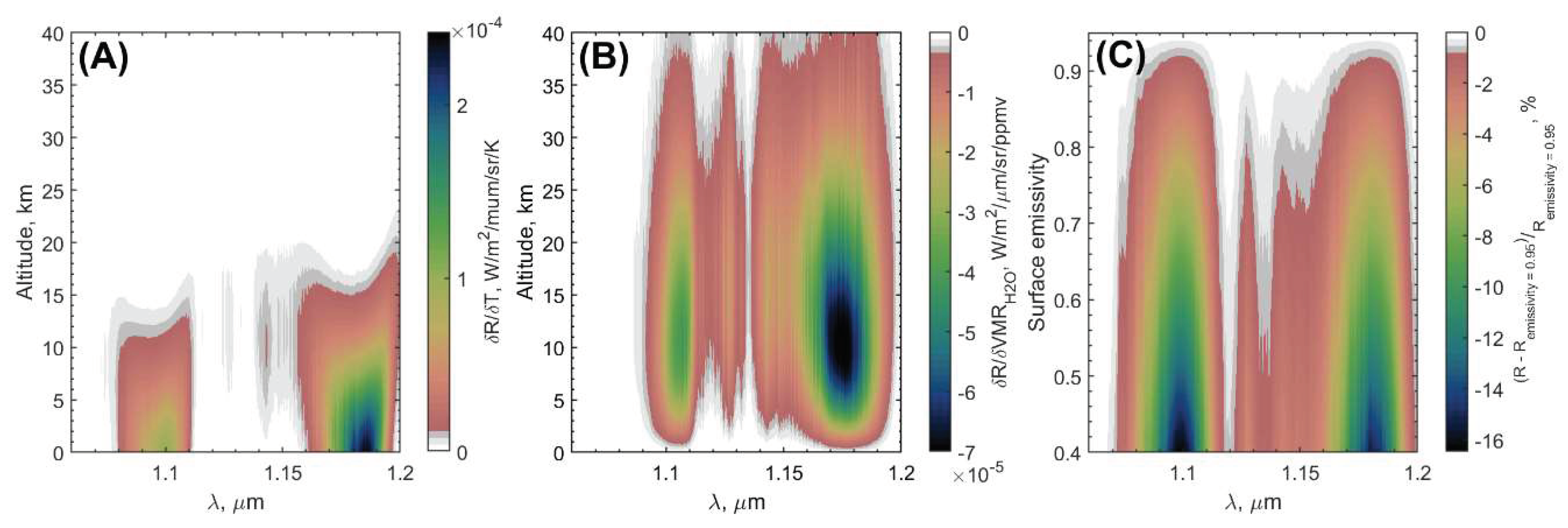
Figure 3.
CO2 and H2O cross-sections computed at the altitude of 10 km (44.2 atm, 651K) computed for different approximations of absorption in far wings. CO2 sub-Lorentzian line profile of Model 1 and Model 2 is based on Ref. [8]. The Voigt profile is used in Model 1 for H2O. H2O absorption in Model 2 is computed based on the H2O far-wings correction MT_CKD model and the HITRAN2020 [47,49]. Model 3 incorporates a sub-Lorentzian line profile for CO2 and the super-Lorentzian line profile for H2O based on Ref. [15,50].
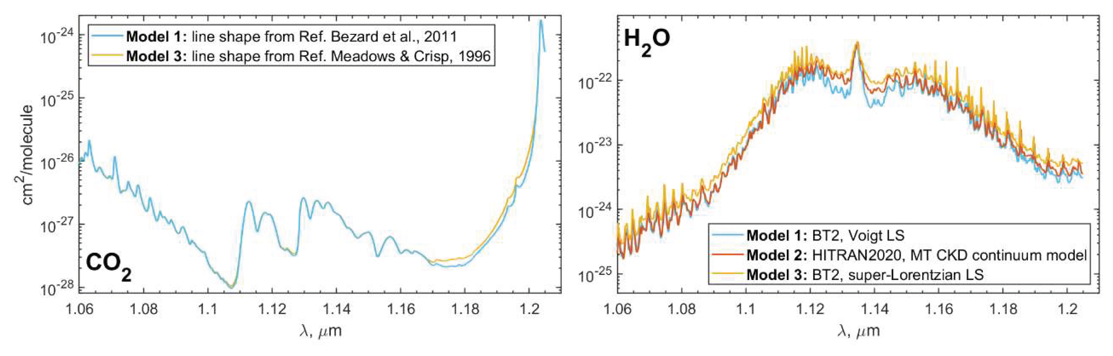
Figure 4.
Examples of measured spectra of 1.1- and 1.18-μm transparency windows fitted by the radiative transfer model computed for the CO2 and H2O line profiles of Model 1, 2 and 3. Surface emissivity is set to 0.95. (A-C) Orbit #0025A10 observed on the 16th of May 2006 at latitude of 7.1°N, longitude of 333.9° and local time of 1H17. (D-F) Orbit #2595A06 observed on the 29th of May 2013 at latitude of 67.7°N, longitude of 358.2° and local time of 23H59. (G-I) Orbit #3098A01 observed on the 6th of October 2014 at latitude of 9.1°S, longitude of 11.2° and local time of 5H05. Experimental data is fitted by the radiative transfer model (Table 2) with the CO2 and H2O absorption line shapes of Model 1 (A, D, G), Model 2 (B, E, H) and Model 3 (C, F, I). The panel legends indicate the surface height in the observed area and the emission angle (∠) value.

Figure 5.
(A) Mean of 52 spectra measured during the #2383A02 orbit fitted by the radiative transfer model computed for the CO2 and H2O line profiles of Model 1, 2 and 3. Surface emissivity is set to 0.95. Orbit #2383A02 observed on the 29th of October 2012 at latitudes from 14.9°S to 33.0°N, longitude of 44.1° and local time of 1H20. (B) Residuals of the Models 1, 2 and 3. (C) Same as Panel A for the spectral range of 1.11-1.16 μm. The panel A legend indicates the emission angle (∠) value.
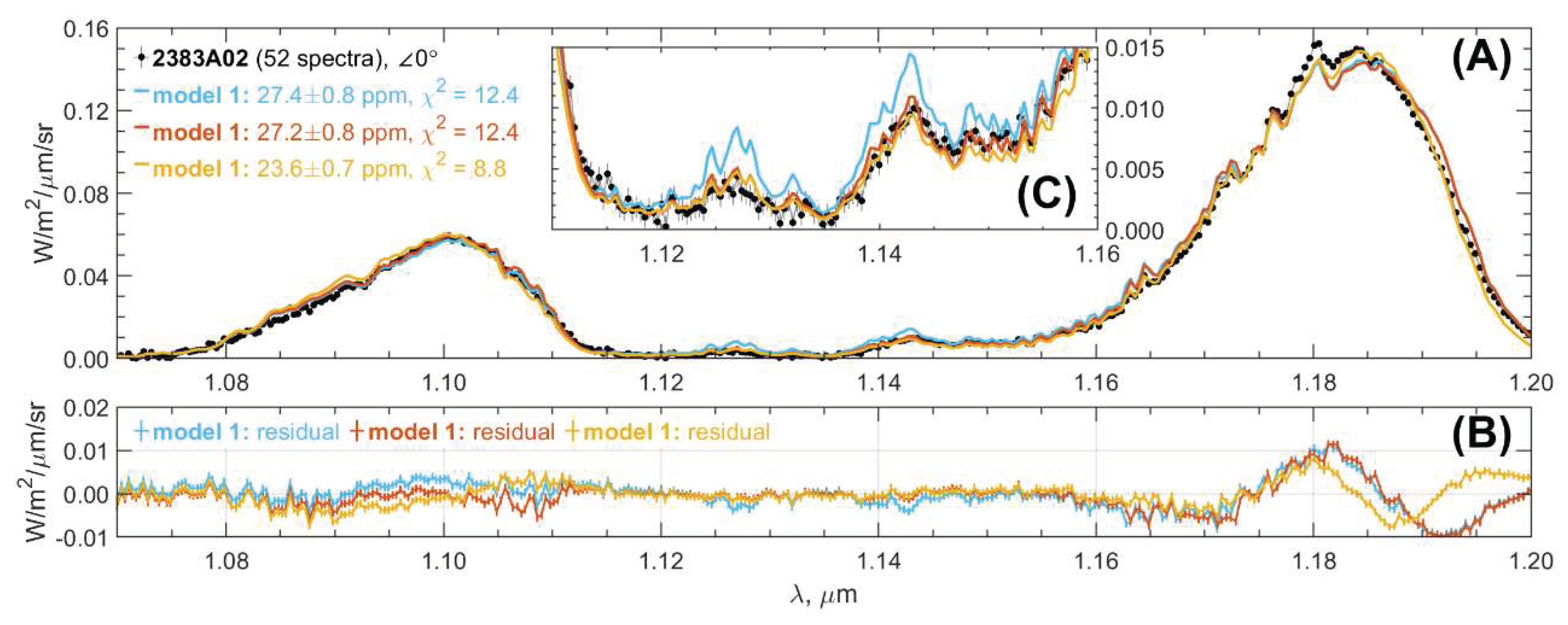
Figure 6.
(A-C) Water vapor volume mixing ratio with respect to latitude. Values were retrieved using the CO2 and H2O absorption line approximation of Model 1 (A), Model 2 (B) and Model 3 (C) presented in detail in Table 2. Color represents the percentage of retrievals in the corresponding VMR bin of 0.5 ppmv relative to all retrievals in the same latitudinal bin of 3°. The black line is the latitudinal distribution of the H2O VMR weighted mean in the latitudinal bin. The magenta line is a similar distribution for a set of values obtained in spectra with signal noise less than 0.006 W/m2/μm/sr and a footprint diameter smaller than 1000 km. Error bars represent a standard deviation within one bin. (D-F) Histogram representing the number of values in one latitudinal bin. Black color corresponds to the latitudinal distribution based on the whole set of observations. Pink color shows distribution of measurements with signal noise <0.006 W/m2/μm/sr and a footprint diameter <1000 km.
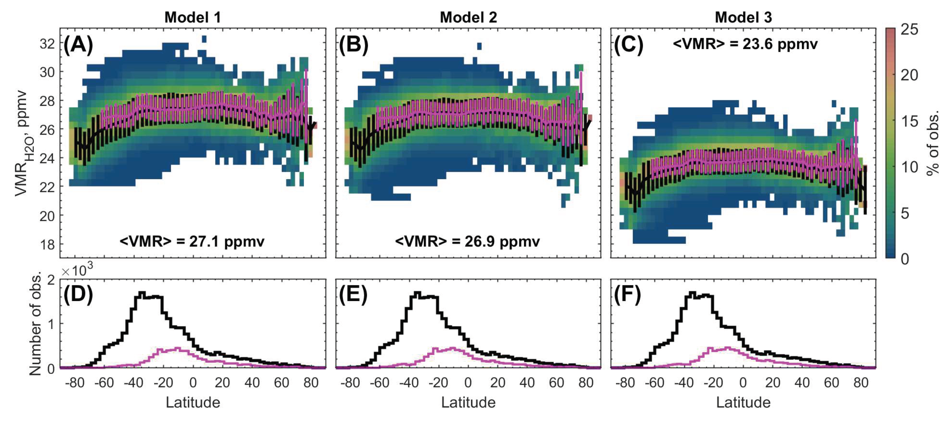
Figure 7.
(A) Geographic distribution of the weighted mean value of H2O VMR obtained on a grid with a 10° latitude and 10° longitude step. (B) Statistics of observations in each 10° latitude-longitude bin. (C) STD of H2O VMR in each 10° latitude-longitude bin. Contour plots are overlaid on the Venus topographic map obtained by the Magellan space mission.
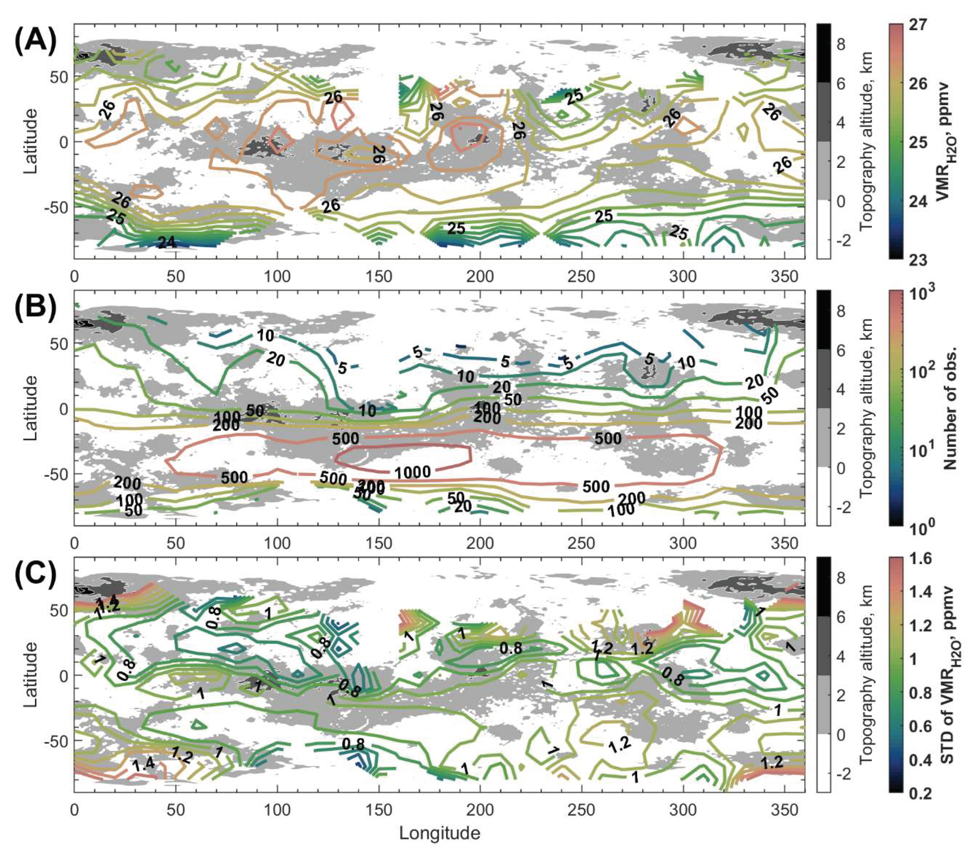
Figure 8.
Examples of measured spectra of 1.1- and 1.18-μm transparency windows fitted by the radiative transfer model computed for the CO2 and H2O line profiles of Model 1, 2 and 3. Surface emissivity is set to 0.4. (A-C) Orbit #0025A10 observed on the 16th of May 2006 at latitude of 7.1°N, longitude of 333.9° and local time of 1H17. (D-F) Orbit #2595A06 observed on the 29th of May 2013 at latitude of 67.7°N, longitude of 358.2° and local time of 23H59. (G-I) Orbit #3098A01 observed on the 6th of October 2014 at latitude of 9.1°S, longitude of 11.2° and local time of 5H05. Experimental data is fitted by the radiative transfer model (Table 2) with the CO2 and H2O absorption line shapes of Model 1 (A, D, G), Model 2 (B, E, H) and Model 3 (C, F, I). The panel legends indicate the surface height in the observed area and the emission angle (∠) value.
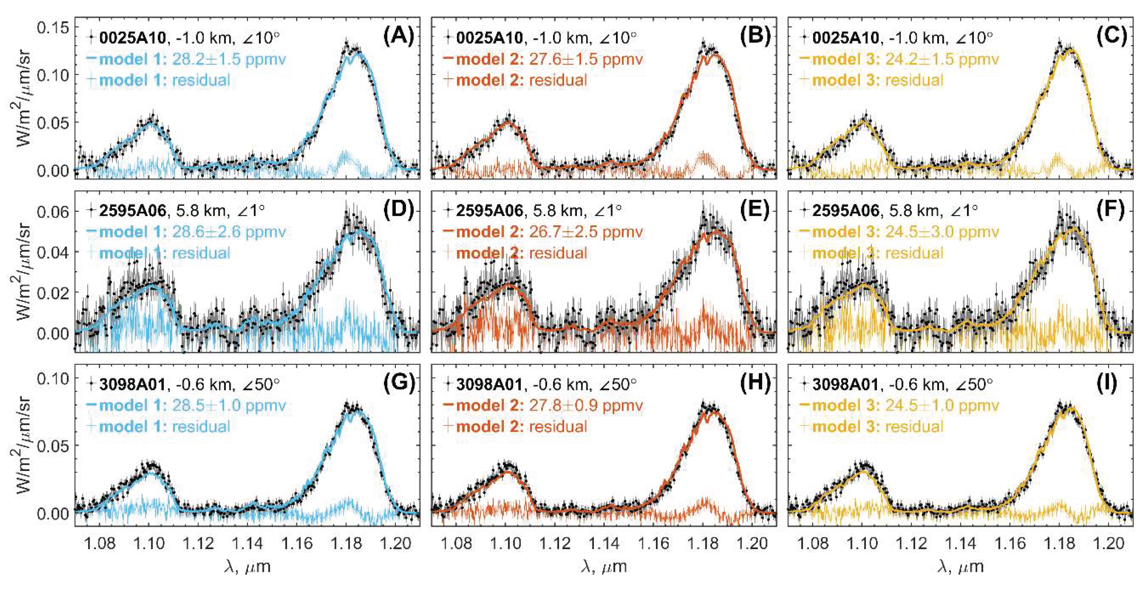

Table 1.
Overview of water vapor measurements in the Venus transparency windows.
| Transparency window | Altitude, km | H2O content, ppmv |
| 1.1 & 1.18 µm | 0-15 | 30 ± 15 [13] 30 ± 15 [14] 45 ± 10 [15] 44 ± 9 [10] 27 ± 6 [16] 32.5 [17] 30 + 10−5 [8] 31 +9−6 [18] 25.7+ 1.4−1.2 (surface emissivity of 0.95) [9] 29.4+ 1.6−1.4 (surface emissivity of 0.6) [9] 29 ± 2 (2009), 27 ± 2 (2010) [11] |
| 1.74 µm | 15-30 | 50 +50-25 [19] 40 [20] 30 ± 7.5 [6] 30 ± 10 [14] 25 ± 5 [21] 33 ± 2 in 2009, 32 ± 2 in 2010 [11] |
| 2.3 µm | 30-45 | ~40 [20] 25 +25-13 [19] 40 (dry profile), 200 (wet profile) [22] 30 ± 6 [6] 30 +15-10 [14] 26 ± 4 [23] 31 ± 2 [24] (22-35) ± 4 [12] ~30-45 (35 km), ~50 (50 km) [25] 34 ± 2 (2009), 33 ± 3 (2010) [11] 27 ± 3.5 [26] |
Table 2.
Summary of parameters and methods used in the radiative transfer model.
| Radiative transfer solver | DISORT4 in the pseudo-spherical geometry with 16 streams [31,32] Line-by-line computation on the wavelength grid with a step of 0.1 cm-1 |
||
| Atmosphere structure | Venus International Reference Atmosphere (VIRA) [33] | ||
| Cloud model | Aerosol number density from Ref. [34] Effective radius of aerosol modes 1, 2, 2’ and 3: 0.3, 1.0, 1.4, 3.65 μm [6,34] Dispersion of aerosol modes 1, 2, 2’ and 3: 1.56, 1.29, 1.23, 1.28 [6,34] Aerosol composition: water solution of H2SO4 with concentration of 75% Aerosol particle shape: spherical H2SO4 refractive index from Ref. [52] Optical depth, single scattering albedo and Legendre series expansion of the scattering phase function are calculated using Mie theory[35] |
||
| Surface emissivity (ε) | 0.95 | ||
| Surface topography | Magellan global topography map [29,30] | ||
| Model 1 | Model 2 | Model 3 | |
| CO2 absorption and molecular scattering | Line list: HITEMP [42] Line profile: sub-Lorenztian of [8] Line cut-off: 250 cm-1 CO2 continuum coef.: 0.30×10⁻⁹ cm-1amagat-2CO2 volume mixing ratio: 0.965 Rayleigh scattering [40,41] |
Line list: HITEMP [42] Line profile: sub-Lorenztian of [8] Line cut-off: 250 cm-1 CO2 continuum coef.: 0.30×10⁻⁹ cm-1amagat-2CO2 volume mixing ratio: 0.965 Rayleigh scattering [40,41] |
Line list: HITEMP [42] Line profile: sub-Lorenztian of [15] Line cut-off: 250 cm-1 CO2 continuum coef.: 0.10×10⁻⁹ cm-1amagat-2CO2 volume mixing ratio: 0.965 Rayleigh scattering [40,41] |
| H2O absorption | Line list: BT2 [43] Line shape: Voigt profile Line cut-off: 180 cm-1 |
Line list: HITRAN2020 [49] Line shape: Voigt profile Line cut-off: 25 cm-1 H2O far-wings correction: MT_CKD model [47] |
Line list: BT2 [43] Line shape: super-Lorenztian [15,50] Line cut-off: 180 cm-1 |
| HDO absorption | Line list: VTT [45] Line shape: Voigt profile Line cut-off: 180 cm-1 D/H ratio: 127 times the terrestrial value |
||
| Model free parameters |
(1) scaling factor applied on particle number density vertical profiles of modes 2, 2’ and 3 (2) H2O volume mixing ratio |
||
Table 3.
Weighted mean of the water vapor volume mixing ratio in the lower atmosphere of Venus retrieved using different approximations of the CO2 and H2O absorption line shape and surface emissivity of 0.95 and 0.4. Radiative transfer model details can be found in Table 2.
Table 3.
Weighted mean of the water vapor volume mixing ratio in the lower atmosphere of Venus retrieved using different approximations of the CO2 and H2O absorption line shape and surface emissivity of 0.95 and 0.4. Radiative transfer model details can be found in Table 2.
| CO2 and H2O line shape model | ε = 0.95 | ε = 0.40 |
| Model 1. H2O Voigt profile | 27.1 ± 1.1 ppmv | 27.7 ± 1.2 ppmv |
| Model 2. H2O line profile correction by the MT_CKD model[47] | 26.9 ± 1.1 ppmv | 27.0 ± 1.1 ppmv |
| Model 3. H2O super-Lorenztian profile [15,49] | 23.6 ± 1.0 ppmv | 24.0 ± 1.0 ppmv |
Disclaimer/Publisher’s Note: The statements, opinions and data contained in all publications are solely those of the individual author(s) and contributor(s) and not of MDPI and/or the editor(s). MDPI and/or the editor(s) disclaim responsibility for any injury to people or property resulting from any ideas, methods, instructions or products referred to in the content. |
© 2025 by the authors. Licensee MDPI, Basel, Switzerland. This article is an open access article distributed under the terms and conditions of the Creative Commons Attribution (CC BY) license (http://creativecommons.org/licenses/by/4.0/).
Copyright: This open access article is published under a Creative Commons CC BY 4.0 license, which permit the free download, distribution, and reuse, provided that the author and preprint are cited in any reuse.


