Submitted:
09 May 2025
Posted:
12 May 2025
You are already at the latest version
Abstract
Nonlinear partial differential equations (PDEs) form the mathematical backbone for modeling phenomena across diverse fields such as physics, biology, engineering, and finance. Traditional numerical methods have limitations, particularly for high- dimensional or parameterized problems, due to the "curse of dimensionality" and computational expense. Artificial Intelligence (AI) is currently a valuable tool and has extensive applications in various fields. AI-driven approaches offer a promising alternative by leveraging machine learning techniques to efficiently approximate solutions, especially in high-dimensional or complex problems. This paper surveys state-of-the-art AI techniques for solving nonlinear PDEs, including Physics-Informed Neural Networks (PINNs), Deep Galerkin Methods (DGM), and Neural Operators. Symbolic computation methods, Hirota bilinear methods, bilinear neural network methods. We explore their theoretical foundations, architectures, advantages, limitations, and applications. Finally, we discuss open challenges and future directions in the field.
Keywords:
Nonlinear partial differential equation
; Artificial Intelligence
; Neural network
; Physics‐Informed
; Symbolic computation
; Bilinear method
1. Introduction
1.1. Background
Nonlinear Partial Differential Equations (PDEs) are used to describe complex, dynamic systems in fluid mechanics, heat transfer, quantum mechanics, and more. These equations model systems where relationships between variables are inherently nonlinear. Their nonlinearity arises from terms like products of derivatives or nonlinear functions of the solution, leading to phenomena such as shocks, turbulence, and chaos. While traditional methods like finite element methods (FEM), finite difference methods (FDM), and spectral methods, solve PDEs by discretizing the problem into manageable subdomains or points, which are powerful for low-dimensional problems, these methods face scalability issues in high-dimensional scenarios or parameterized problems. As a result, they face challenges such as: 1) High-dimensional Problems: Computational cost scales exponentially with dimension. 2) Complex Boundary Conditions: Irregular domains or dynamic boundaries increase solver complexity. 3) Real-Time Applications: Time-sensitive problems (e.g., weather forecasting) require faster solutions.
Artificial Intelligence (AI), particularly Machine Learning (ML) and Deep Learning (DL), offers a new paradigm for addressing these challenges, and provide flexible and scalable alternatives to traditional methods. AI techniques provide efficient, flexible, and scalable methods to approximate, analyze, and solve nonlinear PDEs, often outperforming traditional numerical methods in specific contexts. So AI-driven methods are very important research directions for solving the nonlinear PDEs.
1.2. Motivation
AI methods are attractive due to:
-
Mesh-free nature: Mesh-free nature: AI-driven methods like Physics-Informed Neural Networks (PINNs) and Deep Galerkin Methods (DGM) for solving nonlinear PDEs operate without the need for a predefined grid or mesh. This is a significant departure from traditional numerical methods such as finite element methods (FEM), finite difference methods (FDM), and finite volume methods (FVM), which rely on discretizing the computational domain. Instead:(1) Point-Based Learning: These methods evaluate the solution at scattered points across the domain, which can be sampled randomly or strategically.(2) Neural Representation: The solution u(x,t) is represented as a continuous function, parameterized by the weights of a neural network. For example: PINNs approximate u(x,t) directly by minimizing the residuals at the sampled points. Points do not need to follow any specific spatial organization (e.g., grid).
- High-dimensional scalability: AI-driven methods can handle problems with a large number of spatial, temporal, or parameter dimensions without significantly increasing computational complexity. Traditional numerical approaches, like finite element methods (FEM) or finite difference methods (FDM), struggle with high-dimensional problems due to the curse of dimensionality, whereas AI methods, particularly neural network-based approaches, excel in this regard.
- Learning capabilities: AI-driven approaches, particularly neural network-based models, combine data-driven and physics-informed strategies. This allows them to handle noisy data or unknown parameters, making them well-suited for solving nonlinear PDEs. These capabilities enable them to generalize across complex domains, learn representations of solutions efficiently, and adapt to variations in physical systems.
The remainder of this paper is organized as follows: Section 2 provides the survey of AI Techniques for Nonlinear PDEs, Section 3 give out the survey of AI methods for solving exact analytical solutions of nonlinear PDEs, and Section 4 proposes challenges in AI-driven nonlinear PDE Solvers, Section 5 provides conclusion and future directions.
2. AI Techniques for Nonlinear PDEs
Solving nonlinear PDEs is a complex task due to their inherent challenges, such as nonlinearity, high dimensionality, and the sensitivity of solutions to boundary and initial conditions. Artificial Intelligence (AI) offers a diverse range of techniques for tackling these challenges, providing efficient and scalable methods for solving nonlinear PDEs across different domains. Below, we explore the main AI techniques used for solving nonlinear PDEs, along with their methodologies, applications, and strengths.
2.1. Deep Learning Models for Nonlinear PDEs
2.1.1. Physics-Informed Neural Networks (PINNs)
PINNs [1] are a specific deep learning approach that integrates the governing PDE into the training process. PINNs leverage the physics of the problem by embedding the PDE residual into the loss function.
- Physics-Based Loss Function: Instead of relying solely on data, PINNs directly encode the differential equation into the loss function, ensuring that the model’s predictions adhere to the governing physical laws.
- Example: For solving fluid dynamics problems (e.g., Navier-Stokes equations), PINNs use both boundary/initial conditions and the PDE residual in the loss function to enforce physical constraints, where PINN Loss Function is:
PINNs embed the physical laws governing the PDE as soft constraints into the loss function of a neural network. The network predicts the solution u(x,t) by minimizing the residuals of the PDE, boundary conditions, and initial conditions.
where is to measures how well the solution satisfies the PDE, is to ensure adherence to boundary conditions, is to handle initial conditions.
Its advantages are:
- No need for labeled data.
- Solves forward and inverse problems.
In 2020, Pang et al. [11] extended PINNs to parameter and function inference of integral equations, such as non-local Poisson and non-local turbulence models, and referred to them as non-local PINNs. Non-local physical information neural network nPINNs called parameterized non local pan Laplacian operator. Meng et al. [17] developed the quasi-real physics-informed neural network (PPNN), which decomposes long-time problems into independent short-time problems. In 2022, Jagtap et al. [18] proposed a general framework for neural networks with adaptive activation capabilities called Deep Kronecker neural networks. They also introduced local adaptive activation functions for deep and physical information neural networks with slope recovery [19] and adaptive activation functions to accelerate the convergence of deep and physical information neural networks [20]. Lu et al. [21] developed DeepXDE, a deep learning library for solving differential equations based on the Tensorflow version, and Haghighat et al. [22] developed SciANN, an artificial neural network wrapper based on the Keras/TensorFlow version for deep learning of scientific computing and physical information, at the same time, Zubov et al. [23] developed an automation software package based on Julia called NeuralPDE to implement physical information neural networks. Jin et al. [24] simulated incompressible fluids using physical neural networks. In 2021, Hennigh et al. [25] developed a physical machine learning neural network model development framework (called SimNet) to accelerate simulations across various disciplines in science and engineering. Araz et al. [26] developed a Python package called Elvet, which used machine learning methods to solve differential equations and variational problems, which is a neural network-based solver for differential equations and variation problems. McClenny et al. [27] developed a scalable multi GPU forward and backward solver, TensorDiffEq, based on TensorFlow 2.x, which provides an intuitive Keras style interface for problem domain definition, model definition, and the use of physics aware deep learning methods for physical information neural networks. Koryagin et al. [28] developed a Python framework called PyDEns, which uses neural networks to solve differential equations. Kidger et al. [29] presented Faster ODE Adjointsvia Seminorms, at ICML 2021. Rackauckas et al. [30] described a mathematical object (alled Universal Differential Equations (UDEs) ) as a unified framework for connecting ecosystems. Xiang et al. [31] introduced the adaptive loss balance neural network of incompressible Navier Stokes equation. Peng et al. [32] developed a physics based neural network framework – IDRLnet, which is a Python toolbox used for modeling and solving problems systematically through PINN. IDRLnet provides a structured approach to merge geometric objects, data sources, artificial neural networks, loss metrics, and optimizers into Python. Wang et al. [33] introduced data-driven rogue waves and discovered parameters in the defocused nonlinear Schrödinger equation using PINN deep learning. Xu et al. [34] presented a conditional parameterized and discretized perception neural network for grid based modeling of physical systems. Krishnapriyan et al. [35] introduced the characterization of possible failure modes in physical information neural networks at the 35th Conference on Neural Information Processing Systems (NeurIPS 2021), achieving error reduction of up to 1-2 orders of magnitude. In 2023, Penwarden et al. [36] studied a unified and scalable framework for causal scanning strategies in physical informed neural networks and its temporal decomposition. Yang et al. [37] studied the dynamics of collaborative robots based on human-machine physical interaction and parameter identification based on PINN. Tian et al. [38] studied data-driven non degenerate bound state solitons in multi-component Bose Einstein condensates based on mixed training PINN. Saqlain et al. [39] used PINN to discover the governing equations in discrete systems. Liu et al. [40] studied the adaptive transmission of PINN. Son et al. [41] studied the physical information neural network (AL-PIN) with enhanced Lagrangian relaxation method. Batuwatta Gamage et al. [42] proposed a new physical information neural network method (PINN-MT) to address mass transfer in plant cells during the drying process. Meng et al. [43] proposed a new physics based neural network for reliability analysis of partial differential equations (PINN-FORM). Liu et al. [44] proposed efficient learning of variational physical information neural network based on region decomposition (cv PINN). Pu et al. [45] proposed a new method called Time Segmented Physical Information Neural Networks (PINNs) to study the complex dynamics of one-dimensional quantum droplets by solving the modified Gross Pitaevskii equation. Huang et al. [46] proposed a free physics informed neural network (bif PINN) using boundary and initial conditions to solve non shallow water free surface problems. Penwarden et al. [47] investigated the application of meta learning methods for physics informed neural networks in parameterized partial differential equations. Guo et al. [48] developed a hydraulic tomography physical information neural network (HT-PINN) for inverting two-dimensional large-scale spatial distribution transmittance. P. Villarino et al. [49] developed a new strategy using PINNs to handle the boundary conditions of multidimensional nonlinear parabolic partial differential equations. He et al. [50] combined a multi axis fatigue interface model with a neural network and proposed a physically informed neural network (MFLP-PINN) for life prediction. Zhang et al. [51] integrated computational fluid dynamics with our customized analysis framework based on multi-attribute point cloud dataset and physical information neural network assisted deep learning module. Yin et al. [52] conducted dynamic analysis of optical pulses based on improved PINN, including soliton solutions, strange waves, and parameter discovery of CQ-NLSE. Zhang et al. [53] studied the physics informed neural network with generalized conditional symmetry enhancement and its application in the forward and inverse problems of nonlinear diffusion equations. Peng et al. [54] studied the PINN deep learning method for the Chen Li Liu equation: rogue waves under periodic background. Wang et al. [55] proposed a method of modifying boundary problems through deep learning algorithms for long-term simulation of NLSE rogue waves or aerator solutions with high numerical errors. Zhu et al. [56] used WL tsPINN to predict the dynamic process and model parameters of vector solitons under high-order coupling effects. Li et al. [57] proposed a hybrid training physics informed neural network and studied the strange waves of the Schr ö dinger equation based on it. Pu et al. [58] studied the discovery of vector local waves and parameters in data-driven Manakov systems based on deep learning methods. Zhang et al. [59] applied deep learning methods to study the nonlinear wave solutions of the LPD model describing the evolution of ultra short optical pulses in optical fibers. Meng et al. [17] developed a quasi real physics informed neural network (RPINN) to decompose a long-term problem into many independent short-term problems. Yuan et al. [60] proposed an auxiliary physical neural network (A-PINN) for the forward and inverse problems of nonlinear integral differential equations. Gao et al. [61] proposed a unified framework for solving the forward and inverse problems of PDE control, based on a physical graph neural Galerkin network. Yang et al. [62] proposed Bayesian Physical Informed Neural Networks (B-PINNs) for forward and backward PDE problems on noisy data. Zhang et al. [63] used the continuous symmetry in physical information neural networks to solve the forward and inverse problems of partial differential equations. Guo et al. [64] studied a pre training strategy for solving evolutionary equations based on physical information neural networks. Guan et al. [65] proposed a high-precision and high-efficiency augmented physical informed neural network (DaPINN). Luo et al. [66] proposed a hybrid adaptive (HA) sampling method and a feature embedding layer for PINN for dealing with the accuracy and efficiency of PINNs. Wang et al. [67] extended a multi-layer physics informed neural network and successfully learned data-driven multi soliton solutions, and discovered the coefficients of the fifth order Kaup Kuperschmidt equation using multi soliton data. Tang et al. [68] used a combination of physical informed neural networks and interpolation polynomials to solve nonlinear partial differential equations, and referred to it as Polynomial Interpolation Physical Informed Neural Network (PI-PINN). Zhong et al. [69] used deep physics information neural networks to study the forward and inverse problems of generalized Gross Pitaevskii equations with complex symmetric potentials. Song et al. [70] extended physics informed neural networks to learn data-driven stationary and non-stationary solitons of nonlinear Schrödinger equations. Zhou et al. [71] studied the logarithmic nonlinear Schr ö dinger equation with even and odd time P-symmetric harmonic potentials. Wang et al. [72] applied multi-layer physics informed neural networks for deep learning and successfully studied data-driven peak and periodic peak solutions of some well-known nonlinear dispersion equations with initial boundary conditions. Lin et al. [73] designed a two-stage PINN method that adapts the properties of equations by introducing the characteristics of physical systems into neural networks. Wu et al. [74] conducted a comprehensive study on non-adaptive and residual based adaptive sampling of physics informed neural networks. Qin et al. [75] combined the Weighted Physics Informed Neural Network (WPNN) with the Adaptive Residual Point Distribution (A-WPNN) algorithm to provide an effective deep learning framework for predicting vector soliton solutions and their collisions in coupled nonlinear systems of equations. Lin et al. [76] proposed two physics informed neural network schemes based on Miura transform and obtained new local wave solutions. Chen et al. [77] proposed a physics informed neural network that calculates the most likely transition path by computing the Euler Lagrange equation. Hao et al. [78] used graph neural networks to predict the three-dimensional unsteady multiphase flow field in a coal supercritical fluidized bed reactor. Zhang et al. [79] studied the dual phase field model of composite materials with multiple failures. Wu et al. [80] proposed an unsupervised data-driven method (Seq SVF) for automatically identifying hidden control equations. Peng et al. [66,81] studied graph convolutional neural networks based on physical information for modeling geometric adaptive steady-state natural convection. Li et al. [82] studied the motion estimation and system recognition of mooring buoys based on physical information neural networks. Cui et al. [83] developed numerical inverse scattering transformations for the focusing and defocusing Kundu Eckhaus equations. Mei et al. [273] discussed a unified approach combining finite-volume discretization with physics-informed neural networks to solve heterogeneous PDEs efficiently. Cohen etal. [274] introduced a physics -informed genetic programming approach to discover underlying PDEs from limited and noisy datasets.
The significance of PINNs lies in providing a new approach to handle complex physical problems, especially in the absence of large amounts of data. By combining physical equations and neural networks, PINNs can learn the behavior of a system from a small amount of data and be used for prediction and optimization. This method has potential applications in many fields, including fluid mechanics, materials science, astronomy, and more. The advantage of PINNs is that they can improve prediction accuracy by learning physical equations and can be modeled under different boundary conditions and constraints. In addition, PINNs can improve model performance through adaptive learning and can be combined with traditional numerical methods to provide more accurate and efficient solutions. In summary, the significance of PINNs lies in their provision of a new approach for the fields of science and engineering, which can better handle complex physics problems and still provide accurate predictions and optimizations in situations where data is scarce.
2.1.2. Artificial Neural Networks (ANNs)
Artificial Neural Networks (ANNs) are a fundamental tool in AI-based PDE solvers. These networks, particularly deep feed-forward networks, are used to approximate solutions to nonlinear PDEs. ILagaris et. al [2] demonstrated how feed-forward neural networks can be used to solve both ordinary and partial differential equations, highlighting the effectiveness of ANNs in approximating complex solution. Kumar et al. [271] presented GrADE, a graph-based data-driven solver designed to address time-dependent nonlinear PDEs, showcasing its effectiveness through various applications.
- Nonlinear Mapping: ANNs can approximate highly nonlinear functions due to their layered structure, where each layer transforms the input data nonlinearly.
- Approach: The general approach involves using neural networks to represent the unknown solution u(x,t) of a nonlinear PDE. The network learns to satisfy the PDE by minimizing the residual of the equation during training.
- Example: For a nonlinear heat equation:
,an ANN can be trained to approximate u(x,t) by minimizing the residual:
2.1.3. Deep Galerkin Method (DGM)
DGM [3] solves PDEs by approximating the solution u(x,t) with a deep neural network. The network minimizes the variational form of the PDE by sampling points from the domain. Unlike PINNs, DGM focuses on stochastic sampling, making it particularly suited for high-dimensional PDEs [4]. Beck et al. [5] extended the concept of stochastic methods in solving high-dimensional PDEs, discussing DGM as a specific approach. It emphasizes the use of neural networks and stochastic sampling for efficient computation in high-dimensional settings.
Thus DGM has itself advantages such as Scalability to high-dimensional problems, avoids grid discretization, and efficient sampling strategies for complex domains, and is applied to option pricing in finance (Black-Scholes equation), and reaction-diffusion systems in biology, and so on.
2.1.4. Convolutional Neural Networks (CNNs)
- CNNs are particularly useful in solving PDEs that involve image-based data or spatiotemporal dynamics. These networks can capture local features and spatial patterns efficiently. Zhu et al [7] discussed using CNNs for modeling high-dimensional, spatiotemporal PDEs while enforcing physical constraints, making them ideal for image-based data. Long [8] introduced PDE-Net, which uses CNNs to learn differential operators and approximate solutions to PDEs, showcasing the suitability of CNNs for spatiotemporal dynamics. CNNs are widely used in fluid dynamics, image-based simulation problems, and tasks where the solution exhibits local spatial correlations. They can be used to approximate solution fields directly from data, such as predicting velocity or temperature fields. For example: Solving a convection-diffusion equation using CNNs:
2.2. Neural Operators for PDEs
Neural operators (e.g., Fourier Neural Operators(FNOs), DeepONet) learn the solution mapping of PDEs by directly learning the mapping from input functions to output solutions.
2.2.1. Fourier Neural Operators (FNOs)
FNOs are a class of neural networks that operate in the Fourier space, learning the solution operator of PDEs. They transform the PDE’s spatial domain into the frequency domain, applying learned operations in this domain, making them particularly powerful for nonlinear PDEs. FNOs aim to approximate the solution operator of a PDE, , which maps an input function (e.g., initial condition, boundary condition, or forcing term) to the solution u(x): . There are key characteristics such as (1) Global Representation: FNOs utilize the Fourier transform to represent the function in the frequency domain, capturing both local and global dependencies. (2) Efficiency: The Fourier transform reduces the complexity of handling high-dimensional inputs and outputs. (3) Flexibility: Applicable to parametric, high-dimensional, and nonlinear PDEs.
FNOs are particularly well-suited for solving nonlinear PDEs due to their ability to efficiently capture complex interactions in high-dimensional spaces. Examples include: (1) Navier-Stokes Equations: Modeling fluid flow, including turbulence and vortex dynamics. (2) Burgers’ Equation: Solving for shock waves in nonlinear advection-diffusion processes. (3) Reaction-Diffusion Systems: Simulating pattern formation in chemical and biological systems. (4) Nonlinear Elasticity: Stress-strain modeling for complex materials. (5) Wave Propagation: Solving nonlinear wave equations in acoustics and electromagnetics. Li et al [9] introduced Fourier Neural Operators (FNOs) to demonstrates their ability to efficiently learn solution operators for a variety of parametric PDEs by leveraging the Fourier transform. Kovachki et al. [10] provided a comprehensive overview of neural operators, including FNOs, and their application to solving nonlinear PDEs in various domains by transforming the problem into the Fourier space. Xu et al. [275] considered solving complex spatiotemporal dynamical systems governed by partial differential equations (PDEs) using frequency domain-based discrete learning approaches, such as Fourier neural operators.
2.2.2. DeepONet (Deep Operator Network)
DeepONet is a deep learning framework designed to learn operators between function spaces, enabling it to approximate the solution to a wide class of PDEs. Unlike traditional methods that approximate a solution for a single instance of a PDE, DeepONet learns to approximate the operator itself, enabling rapid solution generation for varying initial conditions, parameters, or source terms. Lu et al [12] introduced DeepONet, leveraging the universal approximation theorem for operators to solve a wide range of PDEs and learning mappings between infinite-dimensional spaces. Wang et al [13] extended DeepONet by incorporating physics-informed learning to improve the efficiency and accuracy of approximating solutions to parametric PDEs. Mouton et al. [269] explored the potential for enhancing a classical deep-learning-based method for solving high-dimensional nonlinear PDEs with suitable quantum subroutines, and constructed a deep-learning architecture based on variational quantum circuits without provable guarantees.
DeepONet consists of two key networks, one for input functions (e.g., initial conditions) and one for output solutions, to learn the operator between these spaces.
(1) Branch Network:
- ✓
- Encodes the input function f into a low-dimensional representation.
- ✓
- Input: Discretized or sampled points of f(x).
- ✓
- Output: Latent features representing the input function.
(2) Trunk Network:
- ✓
- Encodes the evaluation points x into another feature space.
- ✓
- Input: Coordinates where the solution u(x) is to be computed.
- ✓
- Output: Latent features representing the evaluation points.
Finally, combining outputs from the branch and trunk networks to compute the final solution:
where are the outputs of the branch network and are the outouts of the trunk network.
Still, DeepONet has the following key features.
- ✓
- Operator Learning: Directly learns a mapping , where f is an input function (e.g., boundary conditions, initial conditions, or source terms), and u(x) is the solution.
- ✓
- Flexibility: Applicable to linear and nonlinear PDEs, and handles parametric PDEs with variable coefficients or source terms.
- ✓
- Efficiency: Once trained, DeepONet provides real-time solutions for any valid input function fff, bypassing traditional iterative solvers.
- ✓
- Scalability: Applied to high-dimensional PDEs or systems of PDEs.
The loss function can defined as the difference between the predicted solution and the true solution , typically expressed as:
Additional terms may include regularization or physics-informed constraints for PDE consistency.
Applications of DeepONet: Particularly useful for problems where the input function has varying parameters or complex boundary conditions, such as fluid-structure interactions. For example, Navier-Stokes Equations, Burgers’ Equation, Reaction- Diffusion Systems, Nonlinear Elasticity, Quantum Mechanics, and so on.
2.3. Reinforcement Learning for PDEs
Reinforcement Learning (RL) is useful for solving optimal control problems involving nonlinear PDEs, where the goal is to find a control policy that maximizes or minimizes a specific objective function while satisfying the governing PDEs.
- Approach: In this setting, the agent explores possible solutions by interacting with the environment (the PDE), receiving feedback (the objective function), and adjusting its strategy over time. For example, Han et al [14] demonstrated how RL techniques can solve stochastic control problems, which often involve nonlinear PDEs, by approximating value functions using deep learning methods. Rabault et al [15] applied deep reinforcement learning to optimal control problems in fluid dynamics, showcasing its capability to handle nonlinear PDEs governing such systems. Bucci et al [16] explored how RL methods can be adapted for the control of systems described by PDEs, particularly nonlinear dynamics, by framing the control as an optimization problem.
- Applications: Used in control problems such as inverse design of systems governed by PDEs, where the goal is to optimize parameters subject to physical constraints.
- Example: Solving a PDE in a control context, such as optimizing the shape of a membrane subject to dynamic forces.
2.4. Evolutionary Algorithms and Genetic Programming
Evolutionary algorithms, such as genetic programming (GP), are used to discover the form of PDEs or approximate solutions through a process of evolution, and optimize mesh structures or adaptive discretization for numerical solvers, and are particularly, well-suited when the problem involves complex landscapes, unknown parameters, or symbolic representation of solutions.
- Approach: GP evolves mathematical expressions or programs over generations, selecting those that best satisfy the PDE’s conditions. For example, Jin et al [84] reviewed multi-objective optimization techniques, including evolutionary approaches, and discusses their application to discovering and solving PDEs in complex parameter landscapes. Schmid et al [85] introduced an approach using genetic programming to discover symbolic representations of governing equations, including PDEs, from data. Bongard et al [86] demonstrated how genetic programming can uncover the structure of nonlinear dynamical systems, which often involve PDEs, through evolutionary exploration. Deb et al [87] discussed how genetic algorithms can optimize mesh structures and discretization strategies, providing insights for numerical solvers of PDEs.
- Applications: Discovering new, unknown forms of nonlinear PDEs or solving highly complex problems where traditional methods may struggle.
2.5. Hybrid AI-Numerical Methods
Hybrid methods combine AI techniques with traditional numerical solvers (e.g., FEM, FDM), leveraging the strengths of both to improve accuracy and efficiency. This approach can improve accuracy, efficiency, and scalability in applications where classical numerical methods face challenges due to complexity, high-dimensionality, or nonlinearity.
- AI techniques such as deep learning are used to extract important features or optimize initial guesses for numerical solvers. And numerical solvers operate on a reduced basis, enhancing efficiency.
- For data-driven correction, we use numerical methods to solve a coarse version of the PDE, and AI models learn the residual errors and correct the solution iteratively. For example, Raissi et al. [88] demonstrated how AI models, such as neural networks, can be integrated with traditional solvers to approximate fine-scale features by learning residuals. Bar-Sinai et al [89] illustrated how AI can learn corrections to coarse-grid discretizations for PDEs, blending data-driven methods with traditional numerical solvers. Geneva et al. [903] introduced a framework where AI models learn the discrepancy between numerical solutions and true solutions, iteratively refining the accuracy. Kashinath et al. [91] explored hybrid approaches where traditional solvers provide a base solution and AI models learn residuals to enhance the accuracy, especially for real-time applications. Rolfo et al. [270] highlighted the integration of machine learning techniques with numerical methods to solve PDEs more efficiently.
- Applications: In multi-physics problems or where traditional methods are computationally expensive, AI can help reduce the computational burden or enhance accuracy.
2.6. Transfer Learning for Nonlinear PDEs
Transfer learning enables the reuse of previously learned models for solving similar PDEs with different parameters or domains. By leveraging models trained on a related task, transfer learning reduces the amount of data needed for new problems and accelerates learning. Gupta et al [92] discussed the application of transfer learning in Physics-Informed Neural Networks (PINNs) to efficiently solve parametric PDEs by reusing pre-trained models. Li et al [9] also demonstrated how Fourier Neural Operators (FNOs) can employ transfer learning to solve PDEs with different parameter distributions, enhancing efficiency and accuracy. Ruthotto et al [93] highlighted transfer learning’s potential in neural network models inspired by PDEs, reusing knowledge from related domains to accelerate training for new problems. Jin et al [94] showcases the use of transfer learning in neural networks for solving PDEs across different domains or parameter sets, reducing computational costs significantly.
Steps for applying transfer learning to nonlinear PDEs are as follows:
(1). Source Task Training: Select a nonlinear PDE for which you have sufficient training data or can solve numerically. Train a neural network to approximate the solution using supervised learning or physics- informed approaches (e.g., PINNs). Save the trained model, including learned weights and biases.
(2). Target Task Setup: Identify the target PDE, which is related to the source PDE (e.g., similar boundary conditions, domain geometry, or governing equations with slight parameter changes). Define a new model, often based on the architecture used for the source task.
(3). Weight Initialization: Initialize the target model with the weights from the source model. This provides a good starting point, especially for shared patterns between the source and target PDEs.
(4). Fine-Tuning: Train the target model on the new problem using limited data or domain- specific loss functions. Use a smaller learning rate during fine-tuning to retain useful features from the source model.
Example for solving Navier - Stokes Variants:
(A) Source Task: Train on the incompressible Navier-Stokes equations for a specific Reynolds number.
(B) Target Task: Transfer to a higher Reynolds number or a slightly different forcing term.
(5) Implementation:
(A)Use convolutional neural networks (CNNs) or Fourier neural operators (FNOs).
(B)Pre-train on the source task.
(C)Fine-tune on limited data or residuals from the target PDE.
2.7. Supervised Learning for PDE Solutions
In supervised learning, neural networks are trained using labeled data consisting of PDE input conditions (e.g., boundary values) and corresponding solutions. The model learns the mapping from inputs to solutions directly. For example, Raissi et al. [1] demonstrated how neural networks can map input conditions to solutions using supervised learning techniques. Lusch et al. [95] explored using neural networks to discover embedding of nonlinear dynamics, with applications to solving PDEs through supervised learning on labeled datasets of input conditions and solutions. Bhattachary et al. [96] discussed supervised learning techniques for mapping parametric PDE inputs to their solutions, emphasizing neural networks for model reduction. Zhang et al. [97] explored a framework where neural networks learn to solve PDEs without labeled data, using a loss function that incorporates the PDE and boundary conditions. The model generalizes across various domains and boundary conditions, effectively learning the mapping from inputs to solutions. Using supervised learning, its main steps are as follows.
(A). Generate Training Data: We use analytical solutions (if available) or numerical solvers like Finite Difference, Finite Element, or Spectral methods to compute ground truth solutions, and then create input-output pairs (x,t) and u(x,t) over the domain of interest.
(B). Model Design: Input is coordinates x, t; Output: Predicted solution . Then use fully connected neural networks, convolutional neural networks (CNNs), or Fourier neural operators depending on the problem.
(C). Loss Function: The loss function combines data loss and physics loss. Its data loss is to enforce closeness to the ground truth.
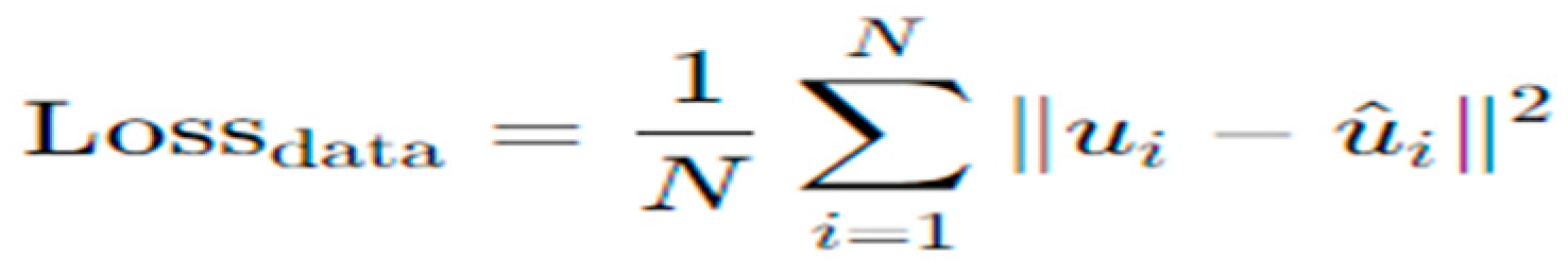 and its physics loss (optional) is to ensure the model satisfies the PDE.
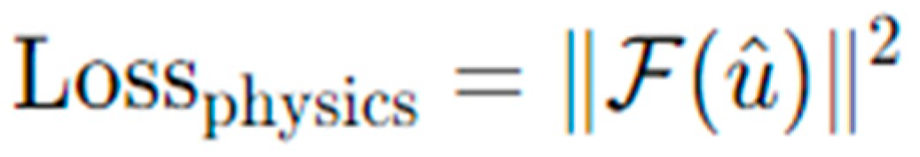
Note that total loss is:

(D) Training: Train the model using a standard optimizer like Adam or SGD, and evaluate performance on validation and test datasets.
(E) Comparison with Physics-Informed Neural Networks (PINNs): Supervised learning requires labeled data (true solutions), while PINNs incorporate the governing equations as part of the loss function, reducing dependency on labeled data. Combining the two methods is also possible for better accuracy.
2.8. Generative Adversarial Networks (GANs)
GANs can be used for solving PDEs by treating the PDE solution process as a generative problem. The generator network produces candidate solutions, and the discriminator network evaluates their validity based on the PDE constraints. For example, Zhu et al. [98] introduced the use of GANs for solving high-dimensional PDEs by generating solutions consistent with physical constraints. Yang et al. [99] explored the use of GANs in inverse problems for PDEs, where the generative model predicts solutions that satisfy the governing equations and boundary conditions. Xie et al [100] developed a framework using GANs to approximate PDE solutions while enforcing physical constraints during training. Sun et al. [101] applied GANs to fluid flow problems governed by PDEs, treating the solution generation as a generative problem with embedded physics constraints. Lu et al. [102] proposed a Physics-Guided Diffusion Model (PGDM) for downscaling PDE solutions. The model generates high-fidelity approximations from low-fidelity inputs, demonstrating the generative approach to solving PDEs under partial observations. Mehdi et al. [103] presented a multi-fidelity physics-informed GAN (MF-PIGAN) that utilizes data from various fidelity levels to solve PDEs. The generative model captures complex solution behaviors across different fidelities, enhancing the accuracy of PDE solutions. These studies illustrated the application of GANs in solving PDEs by modeling the solution process as a generative task, effectively capturing complex solution spaces and integrating physical laws into the learning framework.
GANs have key features as follows: (1) The generator learns to produce solutions that minimize the PDE residuals. (2) The discriminator ensures adherence to physical laws by evaluating whether the generated solution satisfies the PDE. Its applications include: turbulence modeling and other high-dimensional stochastic PDEs, and enhancing resolution in numerical simulations. Its advantages include: (1) Handle complex, high-dimensional PDEs. (2) Provides a probabilistic approach, useful for uncertainty quantification. At the same time, there are challenges such as training GANs is notoriously difficult due to mode collapse and instability, and requires careful design of the discriminator to enforce PDE constraints effectively.
The following is the comprehensive comparison table (see Table 1) for the above techniques across Advantages, Challenges, and Best Use Cases:
3. AI Methods for Solving Exact Analytical Solutions of Nonlinear PDEs
Nonlinear partial differential equations are mathematical models for many practical problems, but their solutions are often very difficult. As we know, the prerequisite for nonlinear partial differential equations to have exact analytical solutions is that the equation is integrable. The classical neural network methods for solving nonlinear partial differential equations (such as PINNs) can only obtain approximate solutions when used to solve nonlinear partial differential equations in integrable systems.
3.1. Symbolic Computation
Symbolic computation is an important mathematical calculation method that utilizes computers to process and manipulate symbols rather than numerical values. The core idea of symbolic computation is to transform mathematical problems into symbolic expressions and solve them through algebraic operations on these symbols. This method has wide applications in fields such as mathematics, physics, and engineering.
Symbolic computation can also be used for equation solving, differentiation, integration, and other operations, which have important applications in mathematical research and engineering practice. In addition to algebraic operations, symbolic computation can also be applied in fields such as calculus, linear algebra, and discrete mathematics. In calculus, symbolic calculations can be used for limit calculations, derivative calculations, integral calculations, and other operations, helping people better understand the concepts and principles of calculus. Although symbolic computing has a wide range of applications in mathematics and engineering, it also faces some challenges and limitations. Firstly, symbol computation requires a significant amount of computational resources and time, especially when dealing with complex symbol expressions. Secondly, the results of symbolic computation are often in symbolic form and need to be further converted into numerical form in order to be applied to practical problems. In addition, the correctness of symbol calculation also needs to be manually verified to ensure the accuracy of the results. Researchers have developed a large number of symbolic computation methods to solve exact analytical solutions of nonlinear sheet differential equations. For example, Hereman et al. [104] proposed two direct methods for solving solitary wave and soliton solutions and applied them to various nonlinear partial differential equations. In addition, there are also F-expansion method [105,106], Darboux transform method [107], homogeneous balance method [108,109,110], Hirota bilinear method [111], Backlund transform [112,113], Tanh expansion method [114], etc. In general, symbolic computation is an important mathematical method that solves various mathematical problems by performing algebraic operations on symbols.
Due to the complexity of the classical analysis method based on bilinear transformation, many existing neural network symbolic computation techniques typically require bilinear transformations to linearize nonlinear PDEs before solving them. However, not all integrable nonlinear PDEs have a bilinear form, so analytical methods based on bilinear transformations may not be applicable to all integrable nonlinear PDEs. In order to address this issue, Zhang et al. [250] proposes a direct neural network symbolic computation method based on nonlinear transformation to directly construct and obtain the exact analytical solutions of nonlinear PDEs. As we know and Kurt has proven in [219], Multilayer perceptron is a universal approximator, it leads that the direct neural network method based on nonlinear transformation will be a universal approach for solving nonlinear partial differential equations (such as (3+1) dimension BLMP equation (see equation (3.1) and (2+1) dimension CBS equation(3.2) below) in integrable systems.


Based on the multiple exponential function method, Darvishi et al. [246] studied the multi wave solutions of equation (3.1). Liu [247] studies the biperiodic soliton solutions of equation (3.1). Liu et al. [241] studied the three wave solution of equation (3.1). Muhammad et al. [248] studied equation (3.2) based on improved (G ’/G) and extended tanh methods. Chen et al. [249] studied the lump solution of the generalized CBS equation system based on the Hirota bilinear form of the generalized CBS equation (3.2). Zhang et al. [250] obtained exact analytical solutions for the (3+1) dimensional BLMP equation and (2+1) dimensional CBS equation by using single hidden layer, double hidden layer, and triple hidden layer neural network models. These results supplement the exact analytical solutions of the (3+1) dimensional BLMP equation and (2+1) dimensional CBS equation in existing literatures
3.2. Hirota Bilinear Methods
Hirota bilinear method is a commonly used mathematical technique in the study of nonlinear partial differential equations. It was developed by Japanese mathematician Hirota [115] and is widely used for analytical solutions and studying the properties of nonlinear partial differential equations. The core idea of Hirota’s bilinear method is to transform nonlinear partial differential equations into a product form of a set of linear partial differential equations. By introducing a special variable transformation and a set of appropriate constraints, the original nonlinear equation can be expressed in the product form of a set of linear equations, commonly referred to as Hirota bilinear equations. The Hirota bilinear method has important applications in the integrability, soliton solutions, conservation laws, and other aspects of nonlinear partial differential equations. It provides a powerful tool for studying nonlinear partial differential equations, enabling researchers to gain a deeper understanding and solve these equations. Yao et al. [116] studied the multi soliton solutions of the (2+1) dimensional Sawada Kotera equation using bilinear methods. Zhang et al. [117] studied the rogue waves and a pair of resonant fringe solitons of the degenerate (3+1) dimensional Jimbo Miwa equation, among others. Wang et al. [118] studied a class of non isospectral and isospectral integrable couplings and their Hamiltonian systems. Yao et al. [119] studied the conservation laws and soliton solutions of the generalized seventh order KdV equation. An et al. [120] studied the general MM-LUMP, high-order respiration, and local interaction solutions of the (2+1) dimensional Sawada Kotera equation. Li et al. [121] studied the extended Hirota bilinear method and the new wave structure of the (2+1) - dimensional Sawada Kotera equation. Wang et al. [122] studied the decay mode solutions of the column/sphere nonlinear Schr ö dinger equation. Zhang et al. [123] studied the dynamic characteristics of vector breathing waves and high-order anomalous waves in the Gerdjikov Ivanov coupling equation. Zhao et al. [124] studied the explosion criterion for the solution of the horizontal viscous primitive equation with horizontal vortex diffusion rate. Wang et al. [125] further improved the F-expansion method and obtained a new exact solution for the Konopelchenko Dubrovsky equation. Xia et al. [126] studied a new family of symbolic calculations and exact soliton like solutions for the Konopelchenko Dubrovsky equation. Zhang et al. [127] applied an improved long wave limit method to study the mechanism of generating high-order rogue waves: NLS case. Zhang et al. [128] studied the periodic solutions of the Lakshman Porcezian Daniel equation and the Whitham modulation equation. Wu et al. [129] studied the degenerate lump chain solutions of the (4+1) dimensional Fokas equation. Yao et al. [130] studied the multi- soliton of non isospectral (2+1) - dimensional soliton equations. Li et al. [131] studied the soliton decomposition process of complex short pulse equations with weighted Sobolev initial data in spatiotemporal soliton regions. Lv et al. [132] studied multiple high-order pole solutions for modified complex short pulse equations. Tian et al. [133] provided an annotation on the Bäcklund transformation of the Harry Dym equation. Zang et al. [134] studied the Bäcklund transformation of a super KdV equation for Kupershmidt, Lax pairs, and related discrete systems. Wen Xiu Ma studied (2+1) dimensional N-soliton solutions and Hirota conditions [135], and proposed an extended bilinear method [136] and linear superposition principle [137,138]. Feng et al. [139] used the Hirota bilinear method to study multiple rogue wave solutions of the (2+1) dimensional YTSF equation. Wazwaz et al. [140] studied the complex simplified Hirota form and Lie symmetry analysis of multiple real soliton and complex soliton solutions of the modified KdV Sine Gordon equation. Wazwaz et al. [141] studied the Hirota direct method and tanh coth method for multi soliton solutions of the seventh order equation of Sawada Kotera Ito. Wazwaz et al. [142] studied the Hirota bilinear method and tanh coth method for multiple soliton solutions of the Sawada Kotera Kadomtsev Petviashvili equation. Osman et al. [143] studied the propagation of light waves in non autonomous Schrödinger Hirota equations with power-law nonlinearity. Zhou et al. [144] studied the composite solutions, Lump, and Lump soliton solutions of the Hirota Satsuma Ito equation. Hua et al. [145] studied the interaction behavior of nonlinear wave generalized (2+1) - dimensional Hirota bilinear equations. Liu et al. [146] studied different complex wave structures described by the variable coefficient Hirota equation in non-uniform optical fibers. Fang et al. [147] studied the interaction solutions of a class of reduced dimensional Hirota bilinear equations. Peng et al. [148] studied the Riemann Hilbert method and PINN algorithm for N-bipolar solutions of non-local Hirota equations under non-zero boundary conditions. In addition, researchers also used this method to study soliton solutions [149,150,151,152,153,154,155], traveling wave solutions [156], non-traveling wave solutions [157], rogue waves [158,159,160,161], rational function solutions [162,163,164,165,166], Lump solutions [167,168,169,170,171,172,173,174,175,176,177,178,179,180,181,182,183,184,185,186,187,188], Lump type solutions [189,190,191,192,193,194,195,196], reactive solutions [197,198,199,200,201,202,203,204,205,206,207,208,209,210,211,212,213], periodic soliton solutions [214,215,216,217,218], and so on.
3.3. Bilinear Neural Network Methods
As we know, the multilayer perceptron model can be seen as a mathematical mapping. Input the independent variable (x; y; z; t), and then map the result f according to the model. In order to obtain exact analytical solutions for nonlinear partial differential equations, Zhang et al [220,221] first proposed a bilinear neural network method (BNNM) for solving exact analytical solutions of nonlinear partial differential equations. This BNNM used the mathematical expression of the multilayer perceptron model as the test function and employ a sign based heuristic function method to solve for the exact analytical solution.
Note that BNNM has some shortcomings such as its trial and error cost with relatively high. Thus, by providing different neural network model structures and some generalized activation functions, many authors constructed various novel heuristic trial functions to improve the BNNM so that BNNM can be extended and applied to high-dimensional equations, integral differential equations, and other nonlinear partial differential equations. For example, by constructing various trial functions with stronger nonlinearity so that BNNM can be applied to more nonlinear equations, Zhang et al [252,253,254,255,256] obtained exact analytical solutions for the (2+1)-dimensional CDGKS like equation, (3+1) - dimensional Jimbo-Miwa equation, BLMP like equation, gBS like equation, and generalized soliton equation. And Zhang et al [258,259] respectively obtained multiple exact solutions for the dimensionally reduced p-gBKP equation and rogue waves, classical lump solutions and generalized lump solutions for Sawada-Kotera-like equation. Qiao et al. [260] obtained three types of periodic solutions of new (3 + 1)-dimensional Boiti-Leon-Manna- Pempinelli equation by BNNM. Gai et al. [222] studied the rich multilayer network model solutions and bright dark solitons of the (3+1) dimensional p-gBLPM equation. Zhu et al. [223] used the bilinear neural network method to solve various solutions of the (2+1) dimensional Hirota Satsuma Ito equation. Lv et al. [224] studied the fission and annihilation phenomena, as well as the interaction phenomena, of respiration/anomalous waves under the non-constant background of two KP equations. Shen et al. [225] used bilinear neural network methods to study the periodic solitons and periodic solutions of the (3+1) dimensional Boiti Leon Manna Pembinelli equation. Qiao et al. [226] used bilinear neural network methods to solve three periodic solutions of the new (3+1) - dimensional Boiti Leon Manna Pempinelli equation. Liu et al. [207] studied the application of multivariate bilinear neural network methods in fractional order partial differential equations. Feng et al. [228] studied the resonant multi soliton and multi anomalous wave solutions of the (3+1) dimensional Kudryashov Sinelshchikov equation and Feng et al. [229] explored the evolution behavior of various wave solutions of the (2+1) dimensional Sharma Tasso Oliver equation. Zeynel et al. [230] used bilinear neural network methods to study the periodic, rogue, and bright dark waves of a new (3+1) dimensional Hirota bilinear equation. Cao et al. [231] studied the respiratory wave, block, and interaction solutions of high-dimensional evolution models. Bai et al. [232] studied high-dimensional evolution models and their anomalous wave solutions, respiratory solutions, and mixed solutions. Zhang et al. [233] studied a neural network-based analytical solver for the Fokker Planck equation. Zhu [257] explored the bilinear residual network method to applied to construct analytical solutions for Nonlinear PDEs.
In order to overcome the shortcomings of BNNM, experts construct various trial functions. Zhang and Li et al. [251] proposed a bilinear residual network method (BRNM) to improve the corresponding trial function. As we know, the activation function of the last layer in fully connected neural network models cannot interact with the neurons inside the network. However, through residual networks, shallow neurons can be transmitted to the inside of the neural network model, achieving internal interactions within the network. By utilizing this characteristic, the trial function constructed using residual network models can provide more interactive results, thereby increasing the probability of obtaining accurate explicit solutions.
This BRNM belongs to the intelligent symbolic computing technology for solving exact analytical solutions of nonlinear partial differential equations, and has the following three advantages: (1). It has higher accuracy than classical neural network methods for solving PDEs, and can obtain 100% accurate analytical solutions; (2). Unify a large number of classic probing letters Numerical method; (3). This lays the foundation and provides a path for the universal solution of symbolic computation for nonlinear partial differential equations in integrable systems. In addition, based on the bilinear neural network method, this method utilizes a residual network model to improve the corresponding trial function. And also Zhang and Li et al. [251] used the bilinear residual network method to applied for the (2+1) dimensional CDGKS equation, and obtained the "3-2-2-1" residual network model and the "3-2-3-1" residual network model, and corresponding exact analytical solutions. More results for various equations can be found at [261]-[268,272].
4. Challenges in AI-Driven Nonlinear PDE Solvers
AI-driven methods for solving nonlinear partial differential equations (PDEs) have demonstrated significant promise, but they also face several challenges. These hurdles range from computational complexity to limitations in generalization and scalability. Addressing these challenges is essential for the widespread adoption of AI-based PDE solvers in real-world applications. Traditional numerical methods may face many issues such as convergence, stability, and computational complexity when dealing with nonlinear equations. In addition, there is currently no universal method for traditional analytical solutions. The method based on neural network symbolic computation (symbolic reasoning) provides a new approach to better solve the challenges of nonlinear partial differential equations, which can make deep learning more interpretable and explainable, providing new ideas for the application of deep learning in scientific research (such as the solving of nonlinear partial differential equations) and engineering applications.
4.1. Challenges
- (1).
- Computational Complexity
(A) Training Time: Training deep neural networks for complex nonlinear PDEs can be computationally expensive, especially for large domains or high-dimensional problems.
Example: PINNs require solving the PDE over many points iteratively, which can result in slow convergence for stiff PDEs like the Navier-Stokes equations.
(B) Memory Requirements: Handling high-dimensional PDEs or large neural networks requires significant memory, especially for methods relying on automatic differentiation.
(C) Resource-Intensive Optimization: Optimizing neural networks involves large-scale matrix operations and gradients computation, which can be resource-intensive for multi-physics PDEs or fine-grained solutions.
- (2).
- Generalization and Extrapolation
(A) Limited Generalization to Unseen Domains: AI models may generalize well within the training domain but struggle to extrapolate to new or unseen domains.
Example: A PINN trained on one geometry may require retraining to adapt to different boundary conditions or domain shapes.
(B) Overfitting to Sampling Points: Poor sampling strategies can lead to overfitting to specific sampled regions, resulting in inaccuracies elsewhere in the domain.
- (3).
- Data Dependency
(A) Data-Driven Models: Methods that rely heavily on data (e.g., supervised neural networks) are only as good as the quality and quantity of available data.
Example: Sparse or noisy experimental data can lead to poorly learned solutions.
(B) Balancing Data and Physics: Striking a balance between data-driven and physics-informed components is challenging, especially for hybrid approaches.
- (4).
- Handling Stiffness and Nonlinearity
(A) Stiff PDEs: characterized by widely varying scales or rapid changes, pose significant training difficulties. Neural networks may struggle to learn stable solutions in such cases.
Example: The Burgers’ equation with a small viscosity parameter results in sharp gradients that are hard to capture.
(B) Strong Nonlinearities: Highly nonlinear PDEs can lead to unstable training and convergence issues. Loss landscapes for such problems may contain many local minima, making optimization challenging.
- (5).
- Loss Function Design and Balancing
(A) Multi-Term Loss Functions: Loss functions in AI-driven solvers often involve multiple terms: residuals, boundary conditions, initial conditions, etc. Balancing these terms during training is non-trivial.
Example: Weighting boundary condition losses too heavily may compromise accuracy in the interior of the domain.
(B) Vanishing Gradients: Loss terms for certain conditions may diminish during training, causing imbalanced optimization and affecting solution accuracy.
- (6).
- Sampling Strategies
(A) Uniform vs Adaptive Sampling: Uniform sampling may miss critical regions like high-gradient areas, while adaptive sampling increases computational complexity.
Example: In turbulent flow simulations, under-sampling near vortices can lead to inaccurate solutions.
(B) High-Dimensional Sampling: Sampling effectively in high-dimensional spaces is challenging, as the number of required samples grows exponentially with dimensionality.
- (7).
- Scalability to Real-World Problems
(A) Large-Scale Domains: Scaling AI solvers to large domains or complex geometries often requires significant computational resources.
Example: Climate models with large domains and multi-scale interactions are computationally demanding.
(B) Multi-Scale and Multi-Physics Problems: Solving PDEs with phenomena occurring across different scales or involving coupled physics (e.g., fluid-structure interactions) remains a challenge.
- (8).
- Numerical Stability and Convergence
(A) Training Instability: Training neural networks for PDE solutions can suffer from instability due to exploding or vanishing gradients.
Example: Oscillatory solutions in wave equations are prone to unstable training dynamics.
(B) Convergence Guarantees: Unlike traditional numerical solvers with well-established convergence theories, AI-driven methods lack robust theoretical guarantees of convergence and accuracy.
- (9).
- Interpretability
(A) Black-Box Nature: Neural networks are often criticized for being black boxes, offering little insight into how solutions are generated or what features are being captured.
Example: Understanding how a neural network captures boundary layer phenomena in fluid dynamics is non-trivial.
(B) Diagnostic Tools: AI-driven solvers lack reliable tools for diagnosing and interpreting errors in learned solutions.
- (10).
- Integration with Existing Frameworks
(A) Hybrid Methods: Integrating AI methods with traditional solvers (e.g., FEM, FDM) introduces compatibility issues.
Example: Transitioning between AI-generated and FEM-based solutions for different regions of a domain can lead to inconsistencies.
(B) Legacy Systems: Many industries rely on well-established numerical frameworks. Adopting AI methods requires significant infrastructure changes.
- (11).
- Lack of Standardization: There is no standardized framework for AI-based PDE solvers, leading to variations in implementations and results. Thus developing unified benchmarks and evaluation metrics is essential for consistency.
- (12).
- Ethical and Practical Concerns
(A) Reliability in Safety-Critical Applications: AI methods must demonstrate high reliability for applications like medical simulations, aerospace engineering, or nuclear reactor modeling.
(B) Energy and Resource Usage: Training large-scale models for PDE solutions can have a significant environmental footprint due to energy consumption.
4.2. Strategies to Address Challenges
(1). Enhanced Sampling: Use adaptive sampling to focus on critical regions, reducing computational cost while maintaining accuracy.
(2). Advanced Optimization Techniques: Leverage advanced optimization methods like second-order optimizers, adaptive learning rates, or reinforcement learning for better training stability.
(3). Hybrid Approaches: Combine AI methods with traditional numerical solvers to exploit the strengths of both.
(4). Explainable AI: Develop interpretable AI models that provide insights into learned solutions and decision-making processes.
(5). Transfer Learning and Pretraining: Use transfer learning to leverage pretrained models, reducing training time for similar PDEs or domains.
(6). Parallelization and High-Performance Computing: Employ GPUs, TPUs, or distributed computing frameworks to accelerate training and inference.
5. Conclusion and Future Directions
AI-driven methods for solving nonlinear PDEs represent a transformative shift in computational science. By combining physics-informed learning with data-driven approaches, these methods offer solutions to problems previously intractable with traditional solvers. However, challenges like interpretability, stability, and scalability need to be addressed for broader adoption.
(1) Hybrid Approaches: Combining AI with traditional numerical methods for enhanced accuracy and stability.
(2) Transfer Learning: Using pretrained models for related PDEs to reduce computational cost.
(3) Explainable AI: Developing interpretable architectures to improve trust in AI solvers.
(4) Real-Time Applications: Optimizing AI solvers for time-critical applications like weather forecasting.
Acknowledgments
This paper is supported by Nature Science Foundation of China under grant number:62466025.
References
- M. Raissi, P.Perdikaris, & G. E.Karniadakis, Physics-informed neural networks: A deep learning framework for solving forward and inverse problems involving nonlinear partial differential equations. Journal of Computational Physics, 2019, 378, 686–707. [CrossRef]
- I. E.Lagaris, A.Likas, & D. I.Fotiadis, Artificial neural networks for solving ordinary and partial differential equations. IEEE Transactions on Neural Networks, 1998, 9(5), 987-1000. [CrossRef]
- J. Sirignano, & K. Spiliopoulos, DGM: A deep learning algorithm for solving PDEs. Journal of Computational Physics, 2018, 375, 1339–1364.
- Han J, Jentzen A, E W. Solving high-dimensional partial differential equations using deep learning, Proceedings of the National Academy of Sciences, 2018, 115(34), 8505-8510. [CrossRef]
- Beck, C., E, W., & Jentzen, A., Machine learning approximation algorithms for high-dimensional fully nonlinear partial differential equations and second-order backward stochastic differential equations. Journal of Nonlinear Science, 2019, 29(4), 1563-1619. [CrossRef]
- Nian, X., & Zhang, Y., A review on reinforcement learning for nonlinear PDEs. Journal of Scientific Computing, 2020, 85, 28.
- Zhu, Y., Zabaras, N., Koutsourelakis, P. S., & Perdikaris, P. (2019). Physics-constrained deep learning for high-dimensional surrogate modeling. Journal of Computational Physics, 394, 56–81. [CrossRef]
- Long, Z., Lu, Y., Ma, X., & Dong, B., PDE-Net: Learning PDEs from data[C], Proceedings of the 35th International Conference on Machine Learning (ICML), 2018. https://proceedings.mlr.press/v80/long18a.html.
- Li, Z., Kovachki, N. B., Azizzadenesheli, K., Liu, B., Bhattacharya, K., Stuart, A., & Anandkumar, A. (2021). Fourier Neural Operator for Parametric Partial Differential Equations. International Conference on Learning Representations (ICLR). https://arxiv.org/abs/2010.08895.
- Kovachki, N. B., Li, Z., Liu, B., Azizzadenesheli, K., Bhattacharya, K., Stuart, A. M., & Anandkumar, A. (2023). Neural operator learning for PDEs. Nature Machine Intelligence, 5, 356–365.
- Pang G, D’Elia M, Parks M, et al. nPINNs: Nonlocal physics-informed neural networks for a parametrized nonlocal universal Laplacian operator. Algorithms and applications, Journal of Computational Physics, 2020, 422: 109760. [CrossRef]
- Lu, L., Jin, P., Pang, G., Zhang, Z., & Karniadakis, G. E., Learning nonlinear operators via DeepONet based on the universal approximation theorem of operators. Nature Communications, 2021,12, Article 6138.
- Wang, S., Yu, X., & Perdikaris, P.. Learning the solution operator of parametric partial differential equations with physics-informed DeepONets. Science Advances, 2021, 7(40), eabi8605. [CrossRef]
- Han, J., & E, W., Deep learning approximation for stochastic control problems. Deep Learning and Applications in Stochastic Control and PDEs Workshop, NIPS. 2016. https://arxiv.org/abs/1611.07422.
- Rabault, J., Kuchta, M., Jensen, A., Reglade, U., & Cerardi, N., Artificial neural networks trained through deep reinforcement learning discover control strategies for active flow control. Nature Machine Intelligence, 2019, 1, 317–324.
- Bucci, M., & Kutz, J. N.. Control of partial differential equations using reinforcement learning. Chaos: An Interdisciplinary Journal of Nonlinear Science, 2021, 31(3), 033148.
- Meng X, Li Z, Zhang D, et al. PPINN: Parareal physics-informed neural network for time- dependent PDEs [J]. Computer Methods in Applied Mechanics and Engineering, 2020, 370: 113250. [CrossRef]
- Jagtap A D, Shin Y, Kawaguchi K, et al. Deep Kronecker neural networks: A general framework for neural networks with adaptive activation functions [J]. Neurocomputing, 2022, 468: 165–180. [CrossRef]
- Jagtap A D, Kawaguchi K, Em Karniadakis G. Locally adaptive activation functions with slop recovery for deep and physics-informed neural networks [J]. Proceedings of the Royal Society A, 2020, 476 (2239): 20200334. [CrossRef]
- Jagtap A D, Kawaguchi K, Karniadakis G E. Adaptive activation functions accelerate convergence in deep and physics-informed neural networks [J]. Journal of Computational Physics, 2020, 404: 109136. [CrossRef]
- Lu L, Meng X, Mao Z, et al. DeepXDE: A deep learning library for solving differential equations [J]. SIAM Review, 2021, 63 (1): 208–228. [CrossRef]
- Haghighat E, Juanes R. SciANN: A Keras/TensorFlow wrapper for scientific computations and physics-informed deep learning using artificial neural networks [J]. Computer Methods in Applied Mechanics and Engineering, 2021, 373: 113552. [CrossRef]
- Zubov K, McCarthy Z, Ma Y, et al. NeuralPDE: Automating Physics-Informed Neural Networks (PINNs) with Error Approximations [J]. arXiv preprint arXiv:2107.09443, 2021.
- Jin X, Cai S, Li H, et al. NSFnets (Navier-Stokes flow nets): Physics-informed neural net works for the incompressible Navier-Stokes equations [J]. Journal of Computational Physics, 2021, 426: 109951. https://www.sciencedirect.com/science/article/pii/S0021999120307257. [CrossRef]
- Hennigh O, Narasimhan S, Nabian M A, et al. NVIDIA SimNet™: An AI-Accelerated Multi-Physics Simulation Framework [C] // Paszynski M, Kranzlmüller D, Krzhizhanovskaya V V, et al. In Computational Science – ICCS 2021, Cham, 2021: 447–461.
- Araz J Y, Criado J C, Spannwosky M. Elvet – a neural network-based differential equation and variational problem solver. 2021.
- McClenny L D, Haile M A, Braga-Neto U M. TensorDiffEq: Scalable Multi-GPU Forward and Inverse Solvers for Physics Informed Neural Networks [J]. arXiv preprint arXiv:2103.16034, 2021.
- Koryagin A, Khudorozhkov R, Tsimfer S. PyDEns: a Python Framework for Solving Differential Equations with Neural Networks [J]. CoRR, 2019, abs/1909.11544. http://arxiv.org/ abs/1909.11544.
- Kidger P, Chen R T Q, Lyons T. “Hey, that’s not an ODE”: Faster ODE Adjoints via Seminorms [J]. International Conference on Machine Learning, 2021.
- Rackauckas C, Ma Y, Martensen J, et al. Universal Differential Equations for Scientific Machine Learning [J]. CoRR, 2020, abs/2001.04385. https://arxiv.org/abs/2001.04385.
- Xiang Z, Peng W, Zheng X, et al. Self-adaptive loss balanced Physics-informed neural networks for the incompressible Navier-Stokes equations[J]. Acta Mechanica Sinica, 2021,37(1):47–52.
- Peng W, Zhang J, Zhou W, et al. IDRLnet: A Physics-Informed Neural Network Library, eprint arXiv:2107.04320, 2021.
- Wang L, Yan Z. Data-driven rogue waves and parameter discovery in the defocusing nonlin ear Schrödinger equation with a potential using the PINN deep learning [J]. Physics Letters A, 2021, 404: 127408. https://www.sciencedirect.com/science/article/pii/S0375960121002723.
- Xu J, Pradhan A, Duraisamy K. Conditionally Parameterized, Discretization-Aware Neural Networks for Mesh-Based Modeling of Physical Systems. arXiv:2012, 2109.09510.
- Krishnapriyan A S, Gholami A, Zhe S, et al. Characterizing possible failure modes in physics informed neural networks [J]. Advances in Neural Information Processing Systems, 2021, 34.
- Penwarden M, Jagtap A D, Zhe S, et al. A unified scalable framework for causal sweeping strategies for Physics-Informed Neural Networks (PINNs) and their temporal decompositions [J]. Journal of Computational Physics, 2023: 112464. [CrossRef]
- Yang X, Zhou Z, Li L, et al. Collaborative robot dynamics with physical human–robot interaction and parameter identification with PINN [J]. Mechanism and Machine Theory, 2023, 189: 105439. [CrossRef]
- Tian S, Cao C, Li B. Data-driven nondegenerate bound-state solitons of multicomponent Bose-Einstein condensates via mix-training PINN [J]. Results in Physics, 2023, 52: 106842. [CrossRef]
- Saqlain S, Zhu W, Charalampidis E G, et al. Discovering governing equations in discrete systems using PINNs [J]. Communications in Nonlinear Science and Numerical Simulation, 2023: 107498. [CrossRef]
- Liu Y, Liu W, Yan X, et al. Adaptive transfer learning for PINN [J]. Journal of Computational Physics, 2023, 490: 112291. [CrossRef]
- Son H, Cho S W, Hwang H J. Enhanced physics-informed neural networks with Augmented Lagrangian relaxation method (AL-PINNs) [J]. Neurocomputing, 2023, 548: 126424. [CrossRef]
- Batuwatta-Gamage C P, Rathnayaka C, Karunasena H C, et al. A novel physics-informed neural networks approach (PINN-MT) to solve mass transfer in plant cells during drying [J]. Biosystems Engineering, 2023, 230: 219–241. [CrossRef]
- Meng Z, Qian Q, Xu M, et al. PINN-FORM: A new physics-informed neural network for reliability analysis with partial differential equation [J]. Computer Methods in Applied Mechanics and Engineering, 2023, 414: 116172. [CrossRef]
- Liu C, Wu H. cv-PINN: Efficient learning of variational physics-informed neural network with domain decomposition [J]. Extreme Mechanics Letters, 2023, 63: 102051.
- Pu J, Chen Y. Complex dynamics on the one-dimensional quantum droplets via time piecewise PINNs [J]. Physica D: Nonlinear Phenomena, 2023, 454: 133851. [CrossRef]
- Huang Y H, Xu Z, Qian C, et al. Solving free-surface problems for non-shallow water using boundary and initial conditions-free physics-informed neural network (bif-PINN) [J]. Journal of Computational Physics, 2023, 479: 112003.
- Penwarden M, Zhe S, Narayan A, et al. A metalearning approach for Physics-Informed Neural Networks (PINNs): Application to parameterized PDEs [J]. Journal of Computational Physics, 2023, 477: 111912. [CrossRef]
- Guo Q, Zhao Y, Lu C, et al. High-dimensional inverse modeling of hydraulic tomography by physics informed neural network (HT-PINN) [J]. Journal of Hydrology, 2023, 616: 128828. [CrossRef]
- P Villarino J, Álvaro Leitao, García Rodríguez J. Boundary-safe PINNs extension: Application to non-linear parabolic PDEs in counterparty credit risk [J]. Journal of Computational and Applied Mathematics, 2023, 425: 115041.
- He G, Zhao Y, Yan C. MFLP-PINN: A physics-informed neural network for multiaxial fatigue life prediction [J]. European Journal of Mechanics - A/Solids, 2023, 98: 104889. [CrossRef]
- Zhang X, Mao B, Che Y, et al. Physics-informed neural networks (PINNs) for 4D hemodynamics prediction: An investigation of optimal framework based on vascular morphology [J]. Computers in Biology and Medicine, 2023, 164: 107287. [CrossRef]
- Yin Y-H, Lü X. Dynamic analysis on optical pulses via modified PINNs: Soliton solutions, rogue waves and parameter discovery of the CQ-NLSE [J]. Communications in Nonlinear Science and Numerical Simulation, 2023, 126: 107441. [CrossRef]
- Zhang Z-Y, Zhang H, Liu Y, et al. Generalized conditional symmetry enhanced physics-informed neural network and application to the forward and inverse problems of nonlinear diffusion equations [J]. Chaos, Solitons & Fractals, 2023, 168: 113169. [CrossRef]
- Peng W-Q, Pu J-C, Chen Y. PINN deep learning method for the Chen–Lee–Liu equation: Rogue wave on the periodic background [J]. Communications in Nonlinear Science and Numerical Simulation, 2022, 105: 106067.
- Wang R-Q, Ling L, Zeng D, et al. A deep learning improved numerical method for the simulation of rogue waves of nonlinear Schrödinger equation [J]. Communications in Nonlinear Science and Numerical Simulation, 2021, 101: 105896. [CrossRef]
- Zhu B-W, Fang Y, Liu W, et al. Predicting the dynamic process and model parameters of vector optical solitons under coupled higher-order effects via WL-tsPINN [J]. Chaos, Solitons & Fractals, 2022, 162: 112441. [CrossRef]
- Li J, Li B. Mix-training physics-informed neural networks for the rogue waves of nonlinear Schrödinger equation [J]. Chaos, Solitons & Fractals, 2022, 164: 112712. [CrossRef]
- Pu J-C, Chen Y. Data-driven vector localized waves and parameters discovery for Manakov system using deep learning approach [J]. Chaos, Solitons & Fractals, 2022, 160: 112182. [CrossRef]
- Zhang Y, Wang L, Zhang P, et al. The nonlinear wave solutions and parameters discovery of the Lakshmanan-Porsezian-Daniel based on deep learning [J]. Chaos, Solitons & Fractals, 2022, 159: 112155. [CrossRef]
- Yuan L, Ni Y-Q, Deng X-Y, et al. A-PINN: Auxiliary physics informed neural networks for forward and inverse problems of nonlinear integro-differential equations [J]. Journal of Computational Physics, 2022, 462: 111260. [CrossRef]
- Gao H, Zahr M J, Wang J-X. Physics-informed graph neural Galerkin networks: A unified framework for solving PDE-governed forward and inverse problems [J]. Computer Methods in Applied Mechanics and Engineering, 2022, 390: 114502. [CrossRef]
- Yang L, Meng X, Karniadakis G E. B-PINNs: Bayesian physics-informed neural networks for forward and inverse PDE problems with noisy data [J]. Journal of Computational Physics, 2021, 425: 109913. [CrossRef]
- Zhang Z Y, Zhang H, Zhang L S, et al. Enforcing continuous symmetries in physics- informed neural network for solving forward and inverse problems of partial differential equations [J]. Journal of Computational Physics, 2023, 492: 112415. [CrossRef]
- Wei Guo J, zhong Yao Y, Wang H, et al. Pre-training strategy for solving evolution equations based on physics-informed neural networks [J]. Journal of Computational Physics, 2023, 489: 112258.
- Long Guan W, han Yang K, sheng Chen Y, et al. A dimension-augmented physics-informed neural network (DaPINN) with high level accuracy and efficiency [J]. Journal of Computational Physics, 2023, 491: 112360.
- Luo, K., Liao, S., Guan, Z. et al. An enhanced hybrid adaptive physics-informed neural network for forward and inverse PDE problems. Appl Intell. , 2025,55, 255. [CrossRef]
- Li Wang X, kang Wu Z, jing Han W, et al. Deep learning data-driven multi-soliton dynamics and parameters discovery for the fifth-order Kaup–Kuperschmidt equation [J]. Physica D: Nonlinear Phenomena, 2023, 454: 133862.
- Ping Tang S, long Feng X, Wu W, et al. Physics-informed neural networks combined with polynomial interpolation to solve nonlinear partial differential equations [J]. Computers & Mathematics with Applications, 2023, 132: 48–62.
- Zhong M, bo Gong S, Tian S-F, et al. Data-driven rogue waves and parameters discovery in nearly integrable PT-symmetric Gross–Pitaevskii equations via PINNs deep learning [J]. Physica D: Nonlinear Phenomena, 2022, 439: 133430.
- Song J, Yan Z Y. Deep learning soliton dynamics and complex potentials recognition for 1D and 2D PT-symmetric saturable nonlinear Schrödinger equations [J]. Physica D: Nonlinear Phenomena, 2023, 448: 133729.
- Jian Zhou Z, Yan Z Y. Solving forward and inverse problems of the logarithmic nonlinear Schrödinger equation with PT-symmetric harmonic potential via deep learning [J]. Physics Letters A, 2021, 387: 127010.
- Wang L, Yan Z Y. Data-driven peakon and periodic peakon solutions and parameter discovery of some nonlinear dispersive equations via deep learning [J]. Physica D: Nonlinear Phenomena, 2021, 428: 133037.
- Lin S N, Chen Y. A two-stage physics-informed neural network method based on conserved quantities and applications in localized wave solutions [J]. Journal of Computational Physics, 2022, 457: 111053.
- Wu C X, Zhu M, Tan Q Y, et al. A comprehensive study of non-adaptive and residual-based adaptive sampling for physics-informed neural networks [J]. Computer Methods in Applied Mechanics and Engineering, 2023, 403: 115671.
- Qin S-M, Li M, Xu T, et al. A-WPINN algorithm for the data-driven vector-soliton solutions and parameter discovery of general coupled nonlinear equations [J]. Physica D: Nonlinear Phenomena, 2023, 443: 133562. [CrossRef]
- Lin S, Chen Y. Physics-informed neural network methods based on Miura transformations and discovery of new localized wave solutions [J]. Physica D: Nonlinear Phenomena, 2023, 445: 133629. [CrossRef]
- Chen X, Duan J, Hu J, et al. Data-driven method to learn the most probable transition pathway and stochastic differential equation [J]. Physica D: Nonlinear Phenomena, 2023, 443: 133559. [CrossRef]
- Hao Y, Xie X, Zhao P, et al. Forecasting three-dimensional unsteady multi-phase flow fields in the coal-supercritical water fluidized bed reactor via graph neural networks [J]. Energy, 2023, 282: 128880. [CrossRef]
- Zhang P, Tan S, Hu X, et al. A double-phase field model for multiple failures in composites [J]. Composite Structures, 2022, 293: 115730. [CrossRef]
- Wu Z, Ye H, Zhang H, et al. Seq-SVF: An unsupervised data-driven method for automatically identifying hidden governing equations [J]. Computer Physics Communications, 2023, 292: 108887. [CrossRef]
- Peng J-Z, Aubry N, Li Y-B, et al. Physics-informed graph convolutional neural network for modeling geometry-adaptive steady-state natural convection [J]. International Journal of Heat and Mass Transfer, 2023, 216: 124593. [CrossRef]
- Li H-W-X, Lu L, Cao Q. Motion estimation and system identification of a moored buoy via physics informed neural network [J]. Applied Ocean Research, 2023, 138: 103677.
- Cui S, Wang Z. Numerical inverse scattering transform for the focusing and defocusing Kundu-Eckhaus equations [J]. Physica D: Nonlinear Phenomena, 2023, 454: 133838. [CrossRef]
- Jin, Y., & Sendhoff, B., Pareto-based multi-objective machine learning: An overview and case studies. IEEE Transactions on Systems, Man, and Cybernetics, Part C: Applications and Reviews, 2009, 38(3), 397-415.
- Schmidt, M., & Lipson, H., Distilling free-form natural laws from experimental data. Science, 2009, 324(5923), 81-85. [CrossRef]
- Bongard, J., & Lipson, H., Automated reverse engineering of nonlinear dynamical systems. Proceedings of the National Academy of Sciences, 2007, 104(24), 9943-9948. [CrossRef]
- Deb, K., & Goyal, M., Optimizing engineering designs using a combined genetic search. Complex Systems, 1997, 9, 213-230.
- Raissi, M., Yazdani, A., & Karniadakis, G. E., Hidden fluid mechanics: Learning velocity and pressure fields from flow visualizations. Science, 2020, 367(6481), 1026-1030. [CrossRef]
- Bar-Sinai, Y., Hoyer, S., Hickey, J., & Brenner, M. P., Learning data-driven discretizations for partial differential equations. Proceedings of the National Academy of Sciences, 2019,116(31), 15344-15349. [CrossRef]
- Geneva, N., & Zabaras, N., Modeling the dynamics of PDE systems with physics-constrained deep auto-regressive networks. Journal of Computational Physics, 2020, 403, 109056. [CrossRef]
- Kashinath, K., Mustafa, M., Albert, A., et al. , Physics-informed machine learning for real-time PDE solutions. Proceedings of the Royal Society A, 2021, 477, 20210400.
- Gupta, S., & Jacob, R. A. (2021).Transfer learning in physics-informed neural networks for solving parametric PDEs. Computer Methods in Applied Mechanics and Engineering, 384, 113938. [CrossRef]
- Ruthotto, L., & Haber, E., Deep neural networks motivated by partial differential equations.Journal of Mathematical Imaging and Vision, 2020, 62, 352–364. [CrossRef]
- Jin, X., Chen, Y., & Li, Z. , Transfer learning for accelerated discovery of PDE solutions using neural networks. Scientific Reports, 2022, 12, Article 3267.
- Lusch S., Kutz J. N., Brunton S. L., Deep learning for universal linear embeddings of nonlinear dynamics, Nature Communications (2018).
- Bhattacharya, K., Hosseini, B., Kovachki, N., & Stuart, A. M., Model reduction and neural networks for parametric PDEs. The SMAI Journal of Computational Mathematics, 2021, 7, 121-157. [CrossRef]
- Xiaoxuan Zhang and Krishna Garikipati, Label-free learning of elliptic partial differential equation solvers with generalizability across boundary value problems, Computer methods in applied mechanics and engineering, 2023, 417, p.116214. [CrossRef]
- Zhu, Y., Zabaras, N., Koutsourelakis, P.-S., & Perdikaris, P., Physics-Constrained Deep Learning for High-Dimensional Surrogate Modeling and Uncertainty Quantification Without Labeled Data. Journal of computational physics, 2019-10, Vol.394, p.56-81. [CrossRef]
- Yang, L., Zhang, D., & Karniadakis, G. E., Physics-Informed Generative Adversarial Networks for Stochastic Differential Equations, SIAM journal on scientific computing, 2020-02, 42 (1). [CrossRef]
- Xie, X., Zheng, C., Li, X., & Xu, L. , Physics-informed generative adversarial networks for solving inverse problems of partial differential equations. Journal of Computational Physics, 2020, 416, 109560.
- Sun, L., Gao, H., Pan, S., & Wang, J.-X., Physics-constrained generative adversarial network for parametric fluid flow simulation. Theoretical and Applied Mechanics Letters, 2020, 10(3), 161-169.
- 2024; Yulong Lu, Wuzhe Xu , Generative Downscaling of PDE Solvers with Physics-Guided Diffusion Models, Journal of scientific computing, 2024, 101 (3), 71. [CrossRef]
- Mehdi Taghizadeh, Mohammad Amin Nabian, Negin Alemazkoor., Multi-Fidelity Physics-Informed Generative Adversarial Network for Solving Partial Differential Equations, Journal of computing and information science in engineering, 2024, 24 (11) 111003. [CrossRef]
- Lu, Lu ; Meng, Xuhui ; Mao, Zhiping ; Karniadakis, George Em, DeepXDE: A Deep Learning Library for Solving Differential Equations, SIAM review, 2021, 63 (1), p.208-228. [CrossRef]
- Hereman W, Nuseir A. Symbolic methods to construct exact solutions of nonlinear partial differential equations [J]. Mathematics and Computers in Simulation, 1997, 43 (1): 13–27. [CrossRef]
- Borg M, Badra N M, Ahmed H M, et al. Solitons behavior of Sasa-Satsuma equation in birefringent fibers with Kerr law nonlinearity using extended F-expansion method [J]. Ain Shams Engineering Journal, 2023: 102290. [CrossRef]
- Rabie W B, Ahmed H M. Cubic-quartic solitons perturbation with couplers in optical metamaterials having triple-power law nonlinearity using extended F-expansion method [J]. Optik, 2022, 262: 169255. [CrossRef]
- Yu J P, Ma W X, Sun S Y L, et al. N–fold Darboux transformation and conservation laws of the modified Volterra lattice [J]. Mod. Phys. Lett. B, 2018, 32: 1850409.
- Abdel Rady A, Osman E, Khalfallah M. The homogeneous balance method and its application to the Benjamin–Bona–Mahoney (BBM) equation [J]. Applied Mathematics and Computation, 2010, 217 (4): 1385–1390.
- Eslami M, Fathi vajargah B, Mirzazadeh M. Exact solutions of modified Zakharov–Kuznetsov equation by the homogeneous balance method [J]. Ain Shams Engineering Journal, 2014, 5 (1): 221–225. [CrossRef]
- Nguyen L T K. Modified homogeneous balance method: Applications and new solutions [J]. Chaos, Solitons & Fractals, 2015, 73: 148–155.
- Hirota R. The direct method in soliton theory [M]. Cambridge University Press, 2004.
- Lü X, Lin F H, Qi F H. Analytical study on a two–dimensional Korteweg–de Vries model with bilinear representation, Bäcklund transformation and soliton solutions [J]. Appl. Math. Model., 2015, 39: 3221–3226.
- Chen S J, Ma W X, Lü X. Bäcklund transformation, exact solutions and interaction behaviour of the (3+1)–dimensional Hirota–Satsuma–Ito–like equation [J]. Commun Nonlinear Sci Numer Simulat, 2020, 83: 105135.
- Wazwaz A-M. The extended tanh method for new compact and noncompact solutions for the KP–BBM and the ZK–BBM equations [J]. Chaos, Solitons Fractals, 2008, 38 (5): 1505–1516.
- Hirota R. The direct method in soliton theory [M]. Cambridge University Press, 2004.
- Yao R X, Li Y, Lou S Y. A new set and new relations of multiple soliton solutions of (2 + 1)- dimensional Sawada–Kotera equation [J]. Communications in Nonlinear Science and Numerical Simulation, 2021, 99: 105820.
- Zhang X E, Chen Y. Rogue wave and a pair of resonance stripe solitons to a reduced (3+1)- dimensional Jimbo–Miwa equation [J]. Communications in Nonlinear Science and Numerical Simulation, 2017, 52: 24–31.
- Wang H F, Zhang Y F. A kind of nonisospectral and isospectral integrable couplings and their Hamiltonian systems [J]. Communications in Nonlinear Science and Numerical Simulation, 2021, 99: 105822.
- Yao R X, Xu G Q, Li Z B. Conservation laws and soliton solutions for generalized seventh order KdV equation [J]. Communications in Theoretical Physics, 2004, 41 (4): 487–492.
- An H L, Feng D L, Zhu y j N v p d d, Hua Xing title= General MM-lump, high-order breather and localized interaction solutions to the 2+12+1-dimensional Sawada–Kotera equation.
- Li Y, Yao R X, Lou S Y. An extended Hirota bilinear method and new wave structures of (2+1)-dimensional Sawada–Kotera equation [J]. Applied Mathematics Letters, 2023, 145: 108760.
- Wang M, Zhang J, Li L. The decay mode solutions of the cylindrical/spherical nonlinear Schrödinger equation [J]. Applied Mathematics Letters, 2023, 145: 108744. [CrossRef]
- Zhang T T, Zhang L D. Dynamic behaviors of vector breather waves and higher-order rogue waves in the coupled Gerdjikov–Ivanov equation [J]. Applied Mathematics Letters, 2023, 143: 108691. [CrossRef]
- Zhao B, Huang D W, Guo B. L., Blow-up criterion of solutions of the horizontal viscous primitive equations with horizontal eddy diffusivity [J]. Applied Mathematics Letters, 2023, 145: 108743.
- Wang D S, Zhang H Q., Further improved F-expansion method and new exact solutions of Konopelchenko–Dubrovsky equation [J]. Chaos, Solitons & Fractals, 2005, 25 (3): 601–610.
- Xia T C, Lü Z S, Zhang H Q., Symbolic computation and new families of exact soliton-like solutions of Konopelchenko-Dubrovsky equations [J]. Chaos, Solitons and Fractals, 2004, 20 (3): 561-566.
- Zhang Z, Yang X Y, Li B, et al. Generation mechanism of high-order rogue waves via the improved long-wave limit method: NLS case [J]. Physics Letters A, 2022, 450: 128395. [CrossRef]
- Zhang Y, Hao H Q, Guo R. Periodic solutions and Whitham modulation equations for the Lakshmanan–Porsezian–Daniel equation [J]. Physics Letters A, 2022, 450: 128369.
- Wu J J, Sun Y J, Li B. Degenerate lump chain solutions of (4+1)-dimensional Fokas equation [J]. Results in Physics, 2023, 45: 106243.
- Yao Y Q, Chen D Y, Zhang D J. Multisoliton solutions to a nonisospectral (2+1)- dimensional breaking soliton equation [J]. Physics Letters A, 2008, 372 (12): 2017–2025.
- Li Z Q, Tian S F, Yang J J, et al. Soliton resolution for the complex short pulse equation with weighted Sobolev initial data in space-time solitonic regions [J]. Journal of Differential Equations, 2022, 329: 31–88.
- Lv C, Liu Q P. Multiple higher-order pole solutions of modified complex short pulse equation [J]. Applied Mathematics Letters, 2023, 141: 108518.
- Tian K, Cui M Y, Liu Q P. A note on Bäcklund transformations for the Harry Dym equation [J]. Partial Differential Equations in Applied Mathematics, 2022, 5: 100352.
- Zang L M, Liu Q P. A super KdV equation of Kupershmidt: Bäcklund transformation, Lax pair and related discrete system [J]. Physics Letters A, 2022, 422: 127794.
- Ma W X. N-soliton solutions and the Hirota conditions in (2+1)-dimensions [J]. Opt Quant Electron, 2020, 52: 511.
- Ma W X. Generalized bilinear differential equations [J]. Stud. Nonlinear Sci., 2011, 2 (4): 140–144.
- Ma W X, Fan E G. Linear superposition principle applying to Hirota bilinear equations [J]. Comput. Math. Appl., 2011, 61: 950–959.
- Ma W X. Bilinear equations, Bell polynomials and linear superposition principle [J]. J. Phys. Conf. Ser., 2013, 411: 012021.
- Feng Y, Bilige S. Multiple rogue wave solutions of (2+1)-dimensional YTSF equation via Hirota bilinear method [J]. Waves in Random and Complex Media, 2021. [CrossRef]
- Wazwaz A M, Kaur L. Complex simplified Hirota’s forms and Lie symmetry analysis for multiple real and complex soliton solutions of the modified KdV-Sine-Gordon equation [J]. Nonlinear Dyn., 2019, 95: 2209–2215.
- Wazwaz A-M. The Hirota’s direct method and the tanh-coth method for multiple-soliton solutions of the Sawada-Kotera-Ito seventh-order equation. [J]. Appl. Math. Comput., 2008, 199 (1): 133–138.
- Wazwaz A-M. The Hirota’s bilinear method and the tanh-coth method for multiple-soliton solutions of the Sawada-Kotera-Kadomtsev-Petviashvili equation [J]. Appl. Math. Comput., 2008, 200 (1): 160–166.
- Osman M S, Lu D C, Khater M M A. A study of optical wave propagation in the nonautonomous Schrödinger–Hirota equation with power–law nonlinearity [J]. Results Phys., 2019, 13: 102157.
- Zhou Y, Manukure S, Ma W X. Lump and lump–soliton solutions to the Hirota–Satsuma–Ito equation [J]. Commun. Nonlinear Sci., 2019, 68: 56–62.
- Hua Y F, Guo B L, Ma W X, et al. Interaction behavior associated with a generalized (2+1)–dimensional Hirota bilinear equation for nonlinear waves [J]. Appl. Math. Modell., 2019, 74: 184–198.
- Liu J G, Osman M S, Zhu W H, et al. Different complex wave structures described by the Hirota equation with variable coefficients in inhomogeneous optical fibers [J]. Appl. Phys. B, 2019, 125:175. [CrossRef]
- Fang T, Wang Y H. Interaction solutions for a dimensionally reduced Hirota bilinear equation [J]. Comput. Math. Appl., 2018, 76: 1476–1485.
- Peng W-Q, Chen Y. N-double poles solutions for nonlocal Hirota equation with nonzero boundary conditions using Riemann–Hilbert method and PINN algorithm [J]. Physica D: Nonlinear Phenomena, 2022, 435: 133274.
- Wazwaz A M. Multiple complex soliton solutions for integrable negative-order KdV and integrable negative-order modified KdV equations [J]. Appl. Math. Lett., 2019, 88: 1–7. [CrossRef]
- Wazwaz A M. A two–mode modified KdV equation with multiple soliton solutions [J]. Appl. Math. Lett., 2019, 70: 1–6. [CrossRef]
- Wazwaz A M. Multiple–soliton solutions for extended (3+1)-dimensional Jimbo-Miwa equations [J]. Appl. Math. Lett., 2017, 64: 21–26.
- Wazwaz A M. Kadomtsev–Petviashvili hierarchy: N-soliton solutions and distinct dispersion relations [J]. Appl. Math. Lett., 2016, 52: 74–79.
- Wazwaz A M, El–Tantawy S A. New (3+1)-dimensional equations of Burgers type and Sharma-Tasso-Olver type: multiple–soliton solutions [J]. Nonlinear Dyn., 2017, 87 (4): 2457–2461.
- Osman M S. One–soliton shaping and inelastic collision between double solitons in the fifth-order variable-coefficient Sawada–Kotera equation [J]. Nonlinear Dyn., 2019, 96: 1491–1496. [CrossRef]
- Osman M S, Wazwaz A M. An efficient algorithm to construct multi-soliton rational solutions of the (2+ 1)-dimensional KdV equation with variable coefficients [J]. Appl. Math. Comput., 2018, 321: 282–289. [CrossRef]
- Lu D C, Seadawy A R, Ali A. Applications of exact traveling wave solutions of Modified Liouville and the Symmetric Regularized Long Wave equations via two new techniques [J]. Results in Physics, 2018, 9: 1403–1410.
- Liua J G, Tian Y, Hu J G. New non-traveling wave solutions for the (3+1)-dimensional Boiti-Leon-Manna-Pempinelli equation [J]. Appl. Math. Lett., 2018, 79: 162-168.
- Cui WY, Zha QL, The third and fourth order rogue wave solutions of the (2+1) dimensional generalized Camassa Holm Kadomtsev Petviashvili equation [J]. Practice and Understanding of Mathematics, 2019, 49 (5), 273-281.
- Lü Z S, Chen Y N. Construction of rogue wave and lump solutions for nonlinear evolution equations [J]. Eur. Phys. J. B, 2015, 88: 187.
- Yang J J, Tian S F, Peng W Q, et al. The lump, lump off and rouge wave solutions of a (3+1)–dimensional generalized shallow water wave equation [J]. Mod. Phys. Lett. B, 2019, 33: 1950190.
- Wu X Y, Tian B, Chai H P, et al. Rogue waves and lump solutions for a (3+1)–dimensional generalized B–type Kadomtsev Petviashvili equation in fluid mechanics [J]. Mod. Phys. Lett. B, 2017, 31 (22): 1750122.
- Du Y H, Yun Y S, Ma W X. Rational solutions to two Sawada Kotera-like equations [J]. Mod. Phys. Lett. B, 2019, 33: 1950108.
- Zhang Y, Dong H H, Zhang X E, et al. Rational solutions and lump solutions to the generalized (3+1)-dimensional Shallow Water-like equation [J]. Comput. Math. Appl., 2017, 73: 246–252.
- Sun Y L, Ma W X, Yu J P, et al. Exact solutions of the Rosenau-Hyman equation, coupled KdV system and Burgers-Huxley equation using modified transformed rational function method [J]. Mod. Phys. Lett. B, 2018, 33: 1850282.
- Feng R Y, Gao X S, Huang Z Y. Rational solutions of ordinary difference equations [J]. Journal of Symbolic Computation, 2008, 43: 746–763.
- Feng R Y, Gao X S. A polynomial time algorithm for finding rational general solutions of first order autonomous ODEs [J]. Journal of Symbolic Computation, 2006, 41: 739–762.
- Ma W X. Lump and interaction solutions to linear (4+1)-dimensional PDSE[J]. Acta Math. Sci., 2019, 39B (2): 498–508.
- Lü J Q, Bilige S D, Chaolu T. The study of lump solution and interaction phenomenon to (2+1)–dimensional generalized fifth–order KdV equation [J]. Nonlinear Dyn., 2018, 91: 1669–1676.
- Lü J Q, Bilige S D. Lump solutions of a (2+1)–dimensional bSK equation [J]. Nonlinear Dyn., 2017, 90: 2119–2124.
- Lü J Q, Bilige S D. The study of lump solution and interaction phenomenon to (2+1) – dimensional Potential Kadomstev – Petviashvili Equation [J]. Anal. Math. Phys., 2018. [CrossRef]
- Lü J Q, Bilige S D, Gao X Q. The study of lump solution and Interaction Phenomenon to (2+1)–dimensional Potential Kadomstev–Petviashvili Equation [J]. Int. J. Nonlinear Sci. Num. Sim., 2018, 20.
- Lü J Q, Bilige S D, Gao X Q, et al. Abundant lump solutions and interaction phenomena to the Kadomtsev–Petviashvili–Benjamin–Bona–Mahony equation [J]. J. Appl. Math. Phys., 2018, 6: 1733–1747.
- Gao X Q, Bilige S D, Lü J Q, et al. Abundant Lump solutions and interaction solutions of The (3+1)–dimensional KP equation [J]. Thermal Science, 2019, 22 (4): 287–294.
- Kaur L, Wazwaz A M. Lump, breather and solitary wave solutions to new reduced form of the generalized BKP equation [J]. Int. J. Numer. Method H., 2019, 29 (2): 569–579. [CrossRef]
- Liu W, Wazwaz A M, Zhang X X. High–order breathers, lumps, and semirational solutions to the (2+1)–dimensional Hirota–Satsuma–Ito equation [J]. Phys. Scr., 2019, 94: 075203.
- Wang H, Wang Y H, Ma W X, et al. Lump solutions of a new extended (2+1)–dimensional Boussinesq equation [J]. Mod. Phys. Lett. B, 2019, 33: 1850376.
- Ma W X, Qin Z Y, Lü X. Lump solutions to dimensionally reduced p–gKP and p–gBKP equations [J]. Nonlinear Dyn., 2016, 84: 923–931.
- Yu J, Ma W X, Chen S T. Lump solutions of a new generalized Kadomtsev-Petviashvili equation [J]. Mod. Phys. Lett. B, 2019, 33: 1950126.
- Manukure S, Zhou Y, Ma W X. Lump solutions to a (2+1)-dimensional extended KP equation [J]. Comput. Math. Appl., 2018, 75: 2414–2419.
- Lü X, Wang J P, Lin F H, et al. Lump dynamics of a generalized two-dimensional Boussinesq equation in shallow water [J]. Nonlinear Dyn., 2018, 91: 1249–1259.
- Gao L N, Zi Y Y, Yin Y H, et al. Bäcklund transformation, multiple wave solutions and lump solutions to a (3 + 1)-dimensional nonlinear evolution equation [J]. Nonlinear Dyn., 2017, 89: 2233–2240.
- Hu C C, Tian B, Yin H M, et al. Dark breather waves, dark lump waves and lump wave–soliton interactions for a (3+1)-dimensional generalized Kadomtsev-Petviashvili equation in a fluid [J]. Comput. Math. Appl., 2019, 78: 166–177.
- Wu X Y, Tian B, Chai H P, et al. Rogue waves and lump solutions for a (3+1)–dimensional generalized B–type Kadomtsev Petviashvili equation in fluid mechanics [J]. Mod. Phys. Lett. B, 2017, 31 (22): 1750122.
- Yang J Y, Ma W X. Lump solutions to the BKP equation by symbolic computation [J]. INT. J. MOD. PHYS. B, 2016, 30: 1640028.
- Chen F P, Chen W Q, Wang L, et al. Nonautonomous characteristics of lump solutions for a (2+1)-dimensional Korteweg-de Vries equation with variable coefficients [J]. Appl. Math. Lett., 2019, 96: 33–39.
- Li W T, Zhang Z, Yang X Y, et al. High-order breathers, lumps and hybrid solutions to the (2+1)-dimensional fifth-order KdV equation [J]. INT. J. MOD. PHYS. B, 2019, 33: 1950255.
- Manukure S, Zhou Y. A (2+1)–dimensional shallow water equation and its explicit lump solutions [J]. INT. J. MOD. PHYS. B, 2019, 33: 1950038. [CrossRef]
- Wang H, Tian S F, Zhang T T, et al. Lump wave and hybrid solutions of a generalized (3+1)-dimensional nonlinear wave equation in liquid with gas bubbles [J]. Front. Math. China, 2019, 14 (3): 631–643. [CrossRef]
- Liu J G. Lump–type solutions and interaction solutions for the (2+1)–dimensional generalized fifth–order KdV equation [J]. Appl. Math. Lett., 2018, 86: 36–41.
- Ma W X, Zhouy Y, Dougherty R. Lump–type solutions to nonlinear differential equations derived from generalized bilinear equations [J]. INT. J. MOD. PHYS. B, 2016, 30: 1640018.
- Liu J G. Lump-type solutions and interaction solutions for the (2+1)–dimensional asymmetrical Nizhnik-Novikov-Veselov equation [J]. Eur. Phys. J. Plus, 2019, 134: 56.
- Ma W X. Lump–Type Solutions to the (3+1)-Dimensional Jimbo-Miwa Equation [J]. Int. J. Sci. Num., 2017, 17: 355–359.
- Fang T, Gao C N, Wang H, et al. Lump–type solution, rogue wave, fusion and fission phenomena for the (2+1)-dimensional Caudrey-Dodd-Gibbon-Kotera-Sawada equation [J]. Modern Physics Letters B, 2019, 33: 1950198.
- Fang T, Wang H, Wang Y H, et al. High-Order Lump-Type Solutions and Their Interaction Solutions to a (3+1)-Dimensional Nonlinear Evolution Equation [J]. Commun. Theor. Phys., 2019, 71: 927–934. [CrossRef]
- Manafian J, Lakestani M. Lump-type solutions and interaction phenomenon to the bidirectional Sawada-Kotera equation [J]. Pramana, 2019, 92: 41. [CrossRef]
- Manafian J, Mohammadi-Ivatloo B, Abapour M. Lump-type solutions and interaction phenomenon to the (2+1)–dimensional Breaking Soliton equation [J]. Appl. Math. Comput., 2019, 356: 13–41. [CrossRef]
- Liu Y Q, Wen X Y. Fission and fusion interaction phenomena of mixed lump kink solutions for a generalized (3+1)-dimensional B-type Kadomtsev-Petviashvili equation [J]. Mod. Phys. Lett. B, 2018, 32: 1850161.
- Dong M J, Tian S F, Wang X B, et al. Lump-type solutions and interaction solutions in the (3+1)-dimensional potential Yu-Toda-Sasa-Fukuyama equation [J]. Anal. Math. Phys., 2018. [CrossRef]
- Zhang R F, Bilige S D, Bai Y X, et al. Interaction phenomenon to dimensionally reduced p–gBKP equation [J]. Mod. Phys. Lett. B, 2018, 32: 1850074.
- Lü J Q, Bilige S D. Diversity of interaction solutions to the (3+1)-dimensional Kadomtsev-Petviashvili-Boussinesq-like equation [J]. Mod. Phys. Lett. B, 2018, 32: 1850311.
- Liu W J, Zhang Y J, Wazwaz A M, et al. Analytic study on triple–S, triple–triangle structure interactions for solitons in inhomogeneous multi-mode fiber [J]. Appl. Math. Comput., 2019, 361: 325–331.
- Zhang J B, Ma W X. Mixed lump-kink solutions to the BKP equation [J]. Comput. Math. Appl., 2017, 74: 591–596.
- Chen J, Yu J P, Ma W X, et al. Interaction solutions of the first BKP equation [J]. Mod. Phys. Lett. B, 2019, 33: 1950191.
- Hu C C, Tian B, Wu X Y, et al. Mixed lump-kink and rogue wave-kink solutions for a (3+1)-dimensional B-type Kadomtsev-Petviashvili equation in fluid mechanics [J]. Eur. Phys. J. Plus, 2018, 133: 40.
- Fang T, Wang H, Wang Y H, et al. Lump–stripe interaction solutions to the potential Yu–Toda–Sasa–Fukuyama equation [J]. Anal. Math. Phys., 2019, 9: 1481–1495.
- Ma W X. Interaction solutions to Hirota–Satsuma–Ito equation in (2+1)–dimensions [J]. Front. Math. China, 2019, 14: 619–629.
- Sun Y L, Ma W X, Yu J P, et al. Lump and interaction solutions of nonlinear partial differential equations [J]. Mod. Phys. Lett. B, 2019, 33: 1950133.
- Ma W X, Yong X L, Zhang H Q. Diversity of interaction solutions to the (2+1)–dimensional Ito equation [J]. Comput. Math. Appl., 2018, 75: 289–295.
- Lin F H, Wang J P, Zhou X W, et al. Observation of interaction phenomena for two dimensionally reduced nonlinear models [J]. Nonlinear Dyn., 2018, 94: 2643–2654.
- Chen S J, Yin Y H, Ma W X, et al. Abundant exact solutions and interaction phenomena of the (2+1)–dimensional YTSF equation [J]. Anal.Math.Phys., 2019. [CrossRef]
- Lan Z Z. Dark solitonic interactions for the (3+1)–dimensional coupled nonlinear Schrödinger equations in nonlinear optical fibers [J]. Optics and Laser Technology, 2019, 113: 462–466.
- Huang L L, Yue Y F, Chen Y. Localized waves and interaction solutions to a (3+1)–dimensional generalized KP equation [J]. Comput. Math. Appl., 2018, 89: 831–844.
- Yue Y F, Huang L L, Chen Y. Localized waves and interaction solutions to an extended (3+1)-dimensional Jimbo–Miwa equation [J]. Appl. Math. Lett., 2019, 89: 70–77.
- Liu J G, He Y. New periodic solitary wave solutions for the (3+1)-dimensional generalized shallow water equation [J]. Nonlinear Dyn., 2017, 90.
- Liu J G, Zhu W H, Zhou L, et al. New periodic solitary wave solutions for the (3+1)–dimensional generalized shallow water equation [J]. Nonlinear Dyn., 2019, 97.
- Zhang R F, Bilige S D, Fang T, et al. New periodic wave, cross–kink wave and the interaction phenomenon for the Jimbo- Miwa- like equation [J]. Comput. Math. Appl., 2019, 78: 754–764.
- Zhao Z L, Chen Y, Han B. Lump soliton, mixed lump stripe and periodic lump solutions of a (2+1)-dimensional asymmetrical Nizhnik-Novikov-Veselov equation [J]. Mod. Phys. Lett. B, 2017, 31: 1750157.
- Zhang R F, Bilige S D. New interaction phenomenon and the periodic lump wave for the Jimbo-Miwa equation [J]. Mod. Phys. Lett. B, 2019, 33: 1950067.
- Hornik K. Approximation capabilities of multilayer feedforward networks [J]. Neural Networks,1991, 4 (2): 251-257. [CrossRef]
- Zhang R F, Bilige S D. Bilinear neural network method to obtain the exact analytical solutions of nonlinear partial differential equations and its application to p–gBKP equatuon [J]. Nonlinear Dyn.,2019, 95: 3041-3048.
- Zhang R F. Multiple exact analytical solutions of nonlinear partial differential equations based on bilinear transformation [D]. Master Thesis,Inner Mongolia University of Technology 2020.
- Gai L T, Bilige S D, Abundant multilayer network model solutions and bright-dark solitons for a (3 + 1)-dimensional p-gBLMP equation [J]. Nonlinear Dynamics, 2021, 106: 867-877.
- Zhu G Z, Wang H L, ao Mou Z, et al. Various solutions of the (2+1)-dimensional Hirota–Satsuma–Ito equation using the bilinear neural network method [J]. Chinese Journal of Physics, 2023, 83:292-305.
- Lv N, Yue Y C, Zhang R F, et al. Fission and annihilation phenomena of breather/rogue waves and interaction phenomena on nonconstant backgrounds for two KP equations [J]. Nonlinear Dynamics, 2023, 111: 10357-10366.
- Shen J L, Wu X Y. Periodic-soliton and periodic-type solutions of the (3+1)-dimensional Boiti–Leon–Manna–Pempinelli equation by using BNNM [J]. Nonlinear Dynamics, 2021, 106: 831–840.
- Qiao J-M, Zhang R-F, Yue R-X, et al. Three types of periodic solutions of new (3 + 1)-dimensional Boiti –Leon-Manna-Pempinelli equation via bilinear neural network method [J]. Mathematical Methods in the Applied Sciences, 2022, 45 (9): 5612–5621.
- Liu J-G, Zhu W-H, Wu Y-K, et al. Application of multivariate bilinear neural network method to fractional partial differential equations [J]. Results in Physics, 2023, 47: 106341. [CrossRef]
- Feng Y Y, Bilige S D. Resonant multi-soliton and multiple rogue wave solutions of (3+1)-dimensional Kudryashov-Sinelshchikov equation [J]. Phys. Scr., 2021, 96: 095217.
- Feng Y Y, Bilige S D, Zhang R F. Evolutionary behavior of various wave solutions of the (2+1)-dimensional Sharma–Tasso–Olver equation [J]. Indian J. Phys., 2022, 96: 2107–2114.
- Zeynel M, Yaşar E. A new (3 + 1) dimensional Hirota bilinear equation: Periodic, rogue, bright and dark wave solutions by bilinear neural network method [J]. Journal of Ocean Engineering and Science, 2022.
- Cao N, Yin X, Bai S, et al. Breather wave, lump type and interaction solutions for a high dimensional evolution model [J]. Chaos, Solitons & Fractals, 2023, 172: 113505.
- Bai S T, jun Yin X, Cao N, et al. A high dimensional evolution model and its rogue wave solution, breather solution and mixed solutions [J]. Nonlinear Dynamics, 2023, 111: 12479–12494.
- Zhang Y, Zhang R F, Yuen K V. Neural network-based analytical solver for Fokker–Planck equation[J]. Engineering Applications of Artificial Intelligence, 2023, 125: 106721. [CrossRef]
- Zhang R F, Li M C, Albishari M, et al. Generalized lump solutions, classical lump solutions and rogue waves of the (2+1)–dimensional Caudrey-Dodd-Gibbon-Kotera-Sawada-like equation [J]. Appl. Math. Comput., 2021, 403: 126201.
- Zhang R F, Li M C, Yin H M. Rogue wave solutions and the bright and dark solitons of the (3+1)-dimensional Jimbo–Miwa equation [J]. Nonlinear Dyn., 2021, 103: 1071-1079.
- Konopelchenko B, Dubrovsky V. Some new integrable nonlinear evolution equations in 2+1 dimensions [J]. Phys. Lett. A, 1984, 102 (1): 15–17. [CrossRef]
- Manafian J, Lakestani M. N-lump and interaction solutions of localized waves to the (2+1)-dimensional variable-coefficient Caudrey-Dodd-Gibbon-Kotera-Sawada equation [J]. J. Geom. Phys., 2020, 150: 103598.
- Cheng X P, Yang Y Q, Ren B, et al. Interaction behavior between solitons and (2+1)-dimensional CDGKS waves [J]. Wave Motion, 2019, 86: 150–161.
- Tang Y, Tao S, Guan Q. Lump solitons and the interaction phenomena of them for two classes of nonlinear evolution equations [J]. Comput. Math. Appl., 2016, 72 (9): 2334–2342. [CrossRef]
- Wazwaz A-M. Painlevé analysis for new (3+1)-dimensional Boiti-Leon-Manna-Pempinelli equations with constant and time-dependent coefficients [J]. International Journal of Numerical Methods for Heat and Fluid Flow, 2020, 30: 4259–4266.
- Liu J G, Du J Q, Zeng Z F, et al. New three-wave solutions for the (3+1)-dimensional Boiti-Leon-Manna-Pempinelli equation [J]. Nonlinear Dyn., 2017, 88.
- Hu L, Gao Y T, Jia T T, et al. Higher-order hybrid waves for the (2 + 1)-dimensional Boiti-Leon-Manna-Pempinelli equation for an irrotational incompressible fluid via the modified Pfaffian technique[J]. Z. Angew. Math. Phys., 2021, 72.
- Gai L T, Ma W X, Li M C. Lump-type solutions, rogue wave type solutions and periodic lump-stripe interaction phenomena to a (3+1)-dimensional generalized breaking soliton equation [J]. Phys. Lett. A, 2020, 384: 126178.
- Chen R D, Gao Y T, Yu X, et al. Periodic-wave solutions and asymptotic properties for a (3+1)-dimensional generalized breaking soliton equation in fluids and plasmas [J]. Mod. Phys. Lett. B, 2021, 35: 2150344.
- Niwas M, Kumar S, Kharbanda H. Symmetry analysis, closed-form invariant solutions and dynamical wave structures of the generalized (3+1)-dimensional breaking soliton equation using optimal system of Lie subalgebra [J]. Ocea. Eng. Sci., 2021. https://www.sciencedirect.com/science/article/pii/S2468013321000693. [CrossRef]
- Darvishi M, Najafi M, Kavitha L, et al. Stair and Step Soliton Solutions of the Integrable (2+1) and (3+1)-Dimensional Boiti-Leon-Manna-Pempinelli Equations [J]. Communications in Theoretical Physics, 2012, 58 (6): 785–794.
- Liu J G. Double-periodic soliton solutions for the (3+1)-dimensional Boiti-Leon- Manna- Pempinelli equation in incompressible fluid [J]. Comput. Math. Appl., 2018, 75: 3604–3613.
- Shakeel M, Mohyud-Din S T. Improved (G’/G)-expansion and extended tanh methods for (2+1)-dimensional Calogero-Bogoyavlenskii-Schiff equation [J]. Alexandria Engineering Journal, 2015, 54 (1): 27–33.
- Chen S T, Ma W X. Lump solutions of a generalized Calogero-Bogoyavlenskii-Schiff equation [J]. Comput. Math. Appl., 2018, 76 (7): 1680-1685.
- Zhang RF, The Neural Network Method for Solving Exact Solutions of Nonlinear Partial Differential Equations[D], Ph.D thesis, Dalian University of Technology, 2023.
- Zhang RF, Li MC, Bilinear residual network method for solving the exactly explicit solutions of nonlinear evolution equations [J]. Nonlinear Dynamics, 2022, 108: 521- 531. [CrossRef]
- Zhang RF, Li MC, Cherraf A, Vadyala SR. The interference wave and the bright and dark soliton for two integro-differential equation by using BNNM [J]. Nonlinear Dynamics, 2023, 111: 8637–8646. [CrossRef]
- Zhang RF, Li MC, Gan JY, Li Q, Lan ZZ. Novel trial functions and rogue waves of generalized breaking soliton equation via bilinear neural network method [J]. Chaos, Solitons & Fractals, 2022, 154: 111692. [CrossRef]
- Zhang RF, Li MC, Albishari M, Zheng FC, Lan ZZ. Generalized lump solutions, classical lump solutions and rogue waves of the (2+1)-dimensional Caudrey Dodd Gibbon Kotera Sawada like equation [J]. Applied Mathematics Computation, 2021, 403:126201.
- Zhang RF, Li MC, Yin HM. Rogue wave solutions and the bright and dark solitons of the (3+1)-dimensional Jimbo–Miwa equation [J]. Nonlinear Dynamics, 2021, 103: 1071–1079. [CrossRef]
- Zhang RF, Bilige SD, Liu JG, Li MC. Bright-dark solitons and interaction phenomenon for p-gBKP equation by using bilinear neural network method [J]. Physica Scripta, 2021, 96:055224. [CrossRef]
- 2024; Zhu Guangzheng, Constructing Analytical Solutions for Nonlinear Partial Differential Equations Using Bilinear Neural Network Method[D], Master Thesis, Guangxi Normal University 2024.
- [258]Zhang RF*, Li MC, Fang T, Zheng FC, Bilige SD. Multiple exact solutions for the dimensionally reduced p-gBKP equation via bilinear neural network method [J]. Modern Physics Letters B, 2022, 36:2150590. [CrossRef]
- [259]Zhang RF*, Li MC, Esmail AM, Zheng FC, Bilige SD. Rogue waves, classical lump solutions and generalized lump solutions for Sawada-Kotera-like equation [J]. International Journal of Modern Physics B, 2022, 36:2250044.
- Qiao JM, Zhang RF*, Yue RX*, Rezazadeh H, Seadawy AR. Three types of periodic solutions of new (3 + 1)-dimensional Boiti–Leon–Manna–Pempinelli equation via bilinear neural network method [J]. Mathematical Methods in Applied Sciences, 2022, 45: 5612-5621.
- Zhang Y, Zhang RF*, Yuen KV*, Rezazadeh H, Seadawy AR. Neural network-based analytical solver for Fokker–Planck equation [J]. Engineering Applications of Artificial Intelligence, 2023, 125: 106721 (SCI Q1). [CrossRef]
- Lv N, Yue YC, Zhang RF, Yuan XG, Wang R. Fission and annihilation phenomena of breather/rogue waves and interaction phenomena on non-constant backgrounds for two KP equations [J]. Nonlinear Dynamics, 2023, 111: 10357-10366 (SCI Q1).
- Gai LT, Qian YH, Zhang RF, Qin YP. Periodic bright-dark soliton, breather-like wave and roguewave solutions to a p-GBS equation in (3+1)-dimensions [J]. Nonlinear Dynamics, 2023, 111: 15335–15346.
- Liu JG, Wazwaz AM, Zhang RF, Lan ZZ, Zhu WH. Breather-wave, multiwave and interaction solutions for the (3+1)-dimensional generalized solition equation [J]. Journal of Applied Analysis & Computation, 2022, 12: 2426-2440.
- Li MY, Bilige SD*, Zhang RF, Han LH. Diversity of interaction phenomenon, crosskink wave, and the bright-dark solitons for the (3+1)-dimensional Kadomtsev-Petviashvili–Boussinesq- like equation [J]. International Journal of Nonlinear Sciences and Numerical Simulation, 2022, 23: F623-634.
- .
- Feng YY, Bilige SD, Zhang RF. Evolutionary behavior of various wave solutions of the (2+1)-dimensional Sharma-Tasso-Olver equation [J]. Indian Journal of Physics, 2022, 96: 2107–2114. [CrossRef]
- Han LH, Bilige SD, Wang XM, Li MY, Zhang RF. Rational Wave Solutions and Dynamics Properties of the Generalized (2+1)-Dimensional Calogero-Bogoyavlenskii-Schiff Equation by Using Bilinear Method [J]. Advances in Mathematical Physics, 2021, 2021: 9295547. [CrossRef]
- Lukas Mouton, Florentin Reiter, Ying Chen, Patrick Rebentrost, Deep-Learning-Based Quantum Algorithms for Solving Nonlinear Partial Differential Equations[J], Physical Review A, 2024,110, 022612. [CrossRef]
- 2024; Rolfo S, Machine Learning-Driven Numerical Solutions to Partial Differential Equations[J], Journal of Applied & Computational Mathematics, 2024, 13(4), 1-2.
- Yash Kumar, Subhankar Sarkar & Souvik Chakraborty, GrADE: A graph based data-driven solver for time-dependent nonlinear partial differential equations[J], Mach. Learn. Comput. Sci. Eng., 2025,1, 7. [CrossRef]
- Abdul Mueed Hafiz, Irfan Faiq & Hassaballah M., Solving partial differential equations using large-data models: a literature review[J], Artif Intell Rev. 2024, 57, 152. [CrossRef]
- Di Mei, Kangcheng Zhou, Chun-Ho Liu, Unified finite-volume physics informed neural networks to solve the heterogeneous partial differential equations[J], Knowledge-Based Systems, 2024, Vol. 295, No. C.
- Benjamin G. Cohen, Burcu Beykal, George M. Bollas, Physics-informed genetic programming for discovery of partial differential equations from scarce and noisy data[J], Journal of Computational Physics, Vol. 514, No. C. [CrossRef]
- Qingsong Xu, Yilei Shi, Jonathan Bamber, Chaojun Ouyang, Xiao Xiang Zhu, Physics- embedded Fourier Neural Network for Partial Differential Equations, arXiv:2024, 2407.11158.
- Sachin Kumar, Setu Rani, Nikita Mann, Analytical Soliton Solutions to a (2 + 1)- Dimensional variable Coefficients Graphene Sheets Equation Using the Application of Lie Symmetry Approach: Bifurcation Theory, Sensitivity Analysis and Chaotic Behavior[J], Qualitative Theory of Dynamical Systems, 2025, 24(2),80. [CrossRef]

Table 1.
Comparison among methods.
| Method | Advantages | Challenges | Best Use Cases |
|---|---|---|---|
| Physics-Informed Neural Networks (PINNs) | - Integrates physical laws into training. - Reduces dependence on labeled data. - Solves forward and inverse problems simultaneously. - Handles high-dimensional PDEs. |
- Computationally expensive, especially for complex systems. - Struggles with stiff PDEs or noisy data. - Requires careful balance of loss terms (physics vs. data). |
- Solving PDEs with limited or no data. - Inverse problems in engineering (e.g., finding material properties). - Multi-physics simulations. |
| Artificial Neural Networks (ANNs) | - General-purpose and flexible. - Effective for both linear and nonlinear mappings. - Can approximate any continuous function (universal approximation theorem). |
- Requires large datasets for accurate training. - Lacks interpretability for scientific applications. - Prone to overfitting on small datasets without regularization. |
- Function approximation in nonlinear systems. - Prediction in time-series models. - General data-driven PDE solutions. |
| Deep Galerkin Method (DGM) | - Efficient for high-dimensional PDEs (avoids grid-based methods). - Trains on scattered data points. - Adaptive and flexible for non-standard boundary conditions. |
- Computational overhead for high-dimensional parameter spaces. - Sensitive to hyperparameter tuning. - May struggle with non-smooth solutions or sharp gradients. |
- Financial modeling (e.g., Black-Scholes equation). - High-dimensional Hamilton-Jacobi-Bellman equations. - Quantum systems with many variables. |
| Convolutional Neural Networks (CNNs) | - Effective for spatially structured data. - Learns hierarchical features (local-to-global patterns). - Translational invariance improves generalization for grid-based data. |
- Limited for irregular geometries or unstructured data. - Requires data in grid format. - Computationally intensive for high resolutions. |
- Image-based PDEs (e.g., seismic inversion). - Structured grid problems (e.g., fluid dynamics on a uniform grid). |
| Fourier Neural Operators (FNOs) | - Captures global dependencies efficiently. - Resolution-independent once trained. - Suitable for high-dimensional problems and long-range correlations. - Fast inference after training. |
- Training can be computationally intensive. - Requires large, diverse datasets for generalization. - Sensitive to frequency mode selection and domain configurations. |
- Parametric PDEs with varying initial/boundary conditions. - Fluid dynamics (e.g., Navier-Stokes equations). - Problems with global spatial dependencies. |
| DeepONet (Deep Operator Network) | - Learns operators, not just solutions. - Real-time inference for varying input functions. - Handles parametric PDEs with ease. - Generalizes across multiple configurations. |
- High computational cost for generating training data. - Requires diverse input-output pairs. - May struggle with rare or out-of-distribution inputs. |
- Learning mappings between function spaces. - Operator discovery in physics. - Control systems with varying conditions. |
| Reinforcement Learning (RL) | - Adaptive to changing environments. - Solves sequential decision-making problems. - Handles dynamic systems and optimization tasks naturally. - Requires no labeled data. |
- High computational cost for training. - Sparse rewards lead to slower convergence. - May struggle with stability in high-dimensional spaces. |
- Optimal control problems. - Adaptive boundary condition modeling. - Dynamic systems with feedback loops. |
| Evolutionary Algorithms (EAs) | - Gradient-free optimization. - Robust to noisy and discontinuous landscapes. - Handles black-box problems effectively. - Avoids local minima traps. |
- Computationally expensive for large search spaces. - Slow convergence for complex or high-dimensional systems. - Requires well-defined fitness functions. |
- Parameter optimization for complex PDE solvers. - Adaptive mesh generation. - Solving non-differentiable or discrete problems. |
| Genetic Programming (GP) | - Discovers symbolic, interpretable solutions. - Effective for problems with missing terms. - Can evolve functional forms directly. - Handles nonlinear dynamics naturally. |
- High computational cost. - Risk of premature convergence. - Requires careful design of crossover and mutation operators. |
- Symbolic PDE discovery. - Closed-form solution generation. - Data-driven discovery of governing equations. |
| Hybrid AI-Numerical Methods | - Combines accuracy of numerical methods with flexibility of AI. - Reduces computational overhead for large-scale problems. - Enhances solution stability and accuracy. |
- Complex implementation. - Integration of AI and traditional solvers can be non-trivial. - Potential for increased computational overhead in hybrid systems. |
- Multiscale simulations. - Coupling turbulence models with AI. - Large-scale fluid dynamics and material simulations. |
| Transfer Learning | - Reduces training time by reusing pre-trained models. - Effective for low-data scenarios. - Leverages knowledge from related domains. |
- Risk of negative transfer if source and target domains differ significantly. - Fine-tuning can introduce overfitting. - Requires careful domain analysis. |
- Low-data PDE problems. - Domain adaptation for scientific applications. - Transfer of pretrained physics models to new scenarios. |
| Supervised Learning | - Straightforward training process. - Handles labeled data effectively. - Can use standard loss functions for clear optimization goals. |
- Requires large labeled datasets. - Prone to overfitting without careful regularization. - Less effective when dealing with partial or noisy data. |
- Classification and regression problems. - Learning mappings for time-dependent or steady-state PDEs. - General numerical PDE approximation. |
| Generative Adversarial Networks (GANs) | - Learns complex distributions effectively. - Generates high-quality synthetic data. - Effective for data augmentation and pattern discovery. - Stochastic PDE modeling is possible. |
- Training instability and mode collapse issues. - Requires careful tuning of generator-discriminator balance. - Computationally expensive to train. |
- Generating synthetic data for physics-based problems. - Stochastic PDEs or uncertainty modeling. - Discovering hidden patterns in datasets. |
Disclaimer/Publisher’s Note: The statements, opinions and data contained in all publications are solely those of the individual author(s) and contributor(s) and not of MDPI and/or the editor(s). MDPI and/or the editor(s) disclaim responsibility for any injury to people or property resulting from any ideas, methods, instructions or products referred to in the content. |
© 2025 by the authors. Licensee MDPI, Basel, Switzerland. This article is an open access article distributed under the terms and conditions of the Creative Commons Attribution (CC BY) license (http://creativecommons.org/licenses/by/4.0/).
Copyright: This open access article is published under a Creative Commons CC BY 4.0 license, which permit the free download, distribution, and reuse, provided that the author and preprint are cited in any reuse.


