Submitted:
09 May 2025
Posted:
10 May 2025
Read the latest preprint version here
Abstract
General covariance is tested controversial after the investigations on gravitational redshift and acceleration. Further inspections on differential geometry indicate the opportunities of inequality of mixed derivatives of bases for the transformations between Riemannian spaces that will then lead to failure of the classical equations of Christoffel symbols, that is the main reason that causes controversies on general covariance. In fact, Christoffel symbols and base derivatives are both valid methodologies for analysis in gravitational fields. Measurable experiments on gravitational redshifts and accelerations have been sponsored to support the theoretical results. Conclusions have been drawn that light speed keeps general covariance in gravitational fields, but light energy momentum would not, while massive matters in gravitational fields do not travel in general covariance. Consequently, inferences on kinematics and relativistic release were put into research, which have got surprising verifications in applications. The problems in classical equations of light ray deflection, time delay of radar echoes and motion of massive matters have been revisited in details, which would help to kick off the errors and help us to find out real kinematics. Relativistic releases reveal the mechanism of evolutions of active galactic nuclei. Relativistic emissions and relativistic absorptions with giant redshifts would have involved with fantastic myths of intrinsic structures of matters that we perhaps know less. Theoretical researches, tremendous experimental and observational verifications would have resulted in comprehensive supports to the conclusions and inferences.
Keywords:
general covariance
; general relativity
; gravitational redshift
; gravitational acceleration
; differential geometry
; covariant differential
; Lagrangian
; energy momentum conservation
; kinematics
; relativistic release
1. Preface
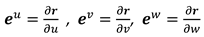
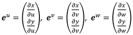
Einstein carried out the equivalence principle
after discussing the equivalence of gravitational mass and inertial mass, and
then he generalized the equivalent principle to create general relativity [1], which predicts same physics in curve space of
gravity geometrization as that in no gravity space, that could be called
general covariance. Theoretically, general covariance should include but not be
limited in the performances of motion inertia, energy and momentum
conservations as well as equilibrium states in complicated systems. However, we
will find out that quite amount of observations and evidences perform against
general covariance.
It is believed that Riemannian geometry has been
employed in general relativity for gravity geometrization [2]. But in fact, a transformation of a space does
not really determine physics, what on earth the realities do. It is said that
it is not the geometry but only the general covariance that matters. In fact,
we could find out plenty of contradictions in classical theory of general
relativity. It could be verified that even the motions of matter’s freefalling
on the Earth cannot be well interpreted in the frames of the classical theory.
So that it is time to sponsor a series of inspections and perceptions to
insight into the topics on general covariance.
The gravitational redshift and gravitational
acceleration are of the two typical effects that gravity acts on the light rays
and massive matters respectively. Hence researches on these topics would be
highly powerful to probe into the investigations and realizations on general
covariance.
To discover realities is more important than to
carry out new equations and theorems.
2. Contradictions on Gravitational Redshift and Acceleration
2.1. Newtonian Gravitational Redshift
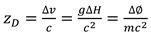
The equation of gravitational redshift can be drawn
via Doppler redshift in a thought experiment that a light ray be emitted from
the ceiling to the bottom or that is reversely performed from bottom to the
ceiling, in a freely falling elevator cabin in a center source field [3]. It could be verified that any observer in the
cabin would detect no frequency shift whatever the ways the light emitted.
Suppose another observer outside the cabin keeping rest so that to have a
relative velocity against the cabin, who will then detect a frequency shift
other than the freefalling observer. What I want to say is that whoever
freefalling will detect no frequency shift, no matter inside or outside the
cabin. It is relative motion that eliminates the gravitational frequency shift.
Once the relative velocities catch up to a relativistic velocity, the
gravitational frequency shift will then cannot be eliminated anymore.
As
a light ray is down ward emitted from a cabin ceiling and at the same time the
cabin is released to freely fall down, the light front should spend a time
interval to reach the bottom that
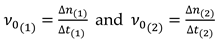
 where is the distance that the light travels from the
start to the end which may approximately equal to the height of the cabin, is light speed.
where is the distance that the light travels from the
start to the end which may approximately equal to the height of the cabin, is light speed.
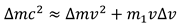
Thus, the cabin velocity increase is
 where is gravitational acceleration, which approximately
equals to gravity case velocity does not reach relativistic level.
We know it exactly has a minus value as its direction pointing to center
source.
where is gravitational acceleration, which approximately
equals to gravity case velocity does not reach relativistic level.
We know it exactly has a minus value as its direction pointing to center
source.
Doppler redshift is frequency shift between two
observers that one has a relative motion to another, to detect frequency. Here
the rest observer outside would have a relative velocity or to the cabin so that when they receive light ray
at the same time with the inner, the Doppler redshift could be calculated as
With the calculation of Doppler redshift we know
that the gravitational redshift has happened in the same value.
Notwithstanding, I prefer to suggest a new methodology to get an equation for gravitational
redshift, in which a proposal should be given that every photon at any position
in a center source field could be assumed to have experienced a travel from a
farthest point to the current position. This attempt may bring about more
physical significances and comprehensive understandings.
A photon in one source field at position with frequency is set to have a virtual primary frequency at a farthest point, so that a so called primary
dynamic energy is
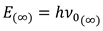 where is Planck’s constant. NB, we are not talking about
quantum character of photons so that photonic mass momentum we are talking
refers to statistic quantities.
where is Planck’s constant. NB, we are not talking about
quantum character of photons so that photonic mass momentum we are talking
refers to statistic quantities.
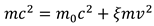
The corresponding dynamic mass comes from the
mass-energy equation is
 where is light speed.
Then the gravitational potential at position , especially as is in weak field with , could be written as
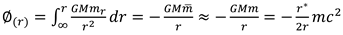 where is gravitational constant, is the mass of the center source, is photonic mass at position , is the mean mass for the integral and it could be approximately replaced by case in weak field, and is Schwarzschild radius written as .
The current dynamic energy is the summation of primary dynamic energy and released potential

Case a light ray travels from positions to , as is shown in Figure 1, gravitational redshift happens.
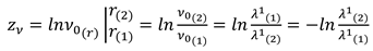
Gravitational redshift will be defined as
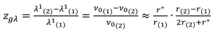
Considering weak field effects, the gravitational redshift is
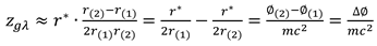
They are the forms of frequency shift of wave length based expression in weak fields, called redshift, where and are wave length and frequency tensors in contra variant space. Of course, a frequency shift could also be defined based on frequency. But we have been used to the forms based on wave length in traditions. In this equation, redshift may go up to more than 1.0, while blueshift must have been limited in -1 to 0. Case in the form of frequency based equations, one could get blueshift greater than 1.0 but redshift limited in -1 to 0.
We could also carry out new forms of frequency shift for conveniences in special discussions, that a differential of wave length based redshift could be defined as
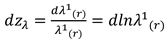
So that the integral form for to
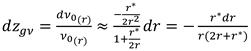
Or a differential form of frequency based
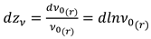
So that
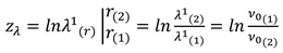
It is said that after the definitions of Eq. (11) and Eq. (13) there is

We have seen that they have shown difference from traditional equation. But for small frequency shift, both the two integral equations could be use instead of traditional equation.
Moreover, with Eq. (7), the gravitational frequency differential
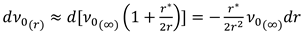
Then the differential frequency shift goes
This equation will be also taken into further discussions in the next sections. In next sections, the subscripts of frequency shift symbols will be neglected for convenience and in most cases we use the concept redshift to present frequency shifts.
2.2. Errors in the Equation of so Called Revisit Gravitational Redshift
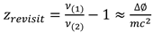
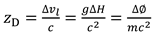
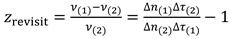
A thought experiment has ever been employed to present the conception of the so called revisit gravitational redshift [3,4], in which a pulse of photons are supposed to be emitted from position 1, lasting for a time interval , and be received at position 2 within a time interval . The world lines of the of photons are shown in Figure 2. We then know that the two drawn lines are literally the world lines of the first photon and the final photon of the light pulse.
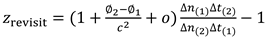
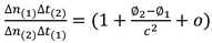
Believing that the two world lines besides the and are parallel, it is known that the time interval equals to that of . As the light frequency being inversely proportional to proper time interval , the proper forms of frequency ratio were written in some textbooks as [3,4]
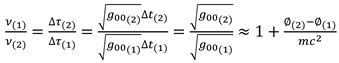 where and are proper frequencies corresponding to position 1 and position 2, is time metric. The right hand side of this equation is an approximate result with Schwarzschild solution of metric in condition that .
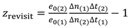
Thus the so called revisit redshift is
It is seemingly that the revisit form of equation for gravitational redshift was worked out.
But there are quite many errors in above equations. (i) The two world lines are belong to the first photon and the final photon, thus they might be controlled by emitter, so that the time intervals between the two lines do nothing with any light frequencies. (ii) Any time intervals between neighboring photons could be randomly assigned, so that these intervals also do nothing with any light frequencies. (iii) Frequency of a photon is the reciprocal of its photonic period and is the intrinsic property of a photon, so that it is independent to its positions relating to other photons and any variation of the frequency will not change its position in the pulse of photons. (iv) Detections of frequencies must involve with wave numbers and time intervals together, this equation has made a mistake by comparing time intervals only.
2.3. Further Investigation into the Revisit Gravitational Redshift
Following the rules in classical frames, the tensor of light wave period is a tensor with upper index
 where, is contra variant period that is described by coordinate time, and is coordinate time lasting in which the number of waves may have traveled across a specific position. And the proper form of wave period
 where, is proper time lasting for number of waves to cross the position. So that there is
 where, is the first component of covariant time base, and it should be noted that the base is a vector but the component is not vector even though it is still a tensor. One can get more understandings for these expressions I would sponsor here and in followings.
In this way, we know that different values of the contra variant period and proper period corresponding to a same physical issue. Then it leads to a frequency tensor
We have seen that, is called covariant tensor traditionally, and is a proper tensor. This may have brought about confusions in that is actually covariant and yet has been named the name. I am not going to change the naming methodology thoroughly right now because that may cause more difficulties and sounds more trivial.
Generally, some pure one-order tensors seem to be infinite small quantities such as, but for , it is divided by , so that it is not an infinite small quantity. As for velocity tensors, they are really mixed tensors.
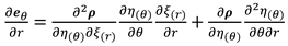
Theoretically, the covariant derivative of a frequency in a falling process into a center source can be written as
 where, is Christoffel symbols.
We know that, as has been presented in Eq. (15), the contra variant derivative is
Let us calculate the Christoffel symbols in Eq. (23) that
The Einstein summation convention has been and will be adopt unless additional declarations.
It is found that only in the condition of there is a nonvanishing item in the bracket of right hand side of Eq. (25), so that with Schwarzschild metrics it turns to be

The covariant derivative will be calculated to be
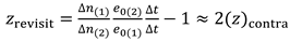
We could get an approximate solution for weak field that

As we have seen, it shows that the values of covariant redshift doubles that of the contra variant redshift.
2.4. Additional Discussions on the Thought Experiment of Freefalling Elevator Cabin
The thought experiment that observer in freefalling elevator cabin will detect no frequency shift is usually employed to discuss the equivalent principle for the support of general covariance. But in fact, that issue does nothing with covariance. It is just because that the gravitational redshift happens to be offset by Doppler redshift. In fact, this experiment is a comprehensive event that relates both to gravitational redshift and gravitational acceleration.
We know that in a freefalling cabin, freefalling observer will not detect any frequency shift no matter the light ray emitter is on the bottom or on the top to emit up or down to the receiver. Nevertheless, even if the light ray is not vertical, freefalling observer would also observe no frequency shift in the cabin.
For a case that a light ray is emitted to the top with an angle to the vertical line
The time interval for light ray from bottom to the top is

And the velocity increase of freefall cabin is
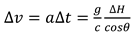
Then the velocity increase component at the direction of light ray
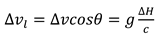
So that we get the Doppler redshift again as
In fact, the Doppler redshift for the detector in freefalling cabin could eliminate the gravitational frequency shift, even if the emitter is either outside of the cabin or with any low initial velocity. The real reason for non-detectable frequency shift in freefalling cabin is that the relative motion formed Doppler redshift just has a minus approximate value of gravitational frequency shift.
I prefer to put forward the case that the gravitational frequency shift cannot be eliminated by Doppler redshift. In the case that cabin has a relativistic initial velocity, the geometrical acceleration is not the total gravitational acceleration again that
Thus, for light rays passing across the cabin there is the Doppler velocity of detector
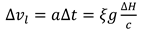
so that
While the gravitational frequency is still the form
 so that in this case

We now know that in some situations in freefalling cabin one could detect frequency shift again, so that the thought experiment cannot support general covariance thoroughly. Of course, one can continue to argue that relativistic motion may bring about more sophisticated conditions on frequency shift.
2.5. An Investigation into Gravitational Acceleration
For a freefalling massive matter in gravitational field, the component of the velocity at the direction of radius of center source is

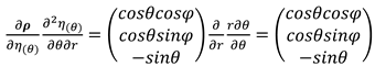
There is the covariant derivative at one of coordinate direction
Because , and , where is the nonvanishing component of the base . Thus, the covariant derivative by is
 where, is the contra variant acceleration of the matter, is light speed.
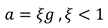
NB, accelerations we have and will discuss refer to geometrical accelerations, which will be something different from gravity , in that the latter sometimes may also be called gravitational accelerations in some writings but in fact matters may not experience accelerating up to that.
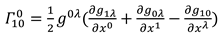
With the equation of Christoffel symbols
case in this equation, there is . Then considering the condition of , it is
In this condition, only in the case of there is the nonvanishing item in the bracket of right hand side, so that

And with , Eq. (40) turns to be
As a matter freefalls on to the earth, its acceleration could be calculated to be
Thus, there is the weak field solution

2.6. Discussions and Controversies
Now we have got more complex results that the revisit gravitational redshift calculated doubles that of contra variant value while covariant acceleration of freefalling goes to zero. The latter seems to fit with general covariance but the previous does not. And there is still a problem that revisit gravitational redshift solved in the way of covariant derivation goes contradictory to classical solution. Moreover, the minus form of also involves more matters that have cause the result of zero acceleration, deserving further discussions in next sections.
It is extraordinary that the covariant derivative of light frequency goes nonvanishing in the view of general covariance. Even more, it is investigated that covariant derivative analysis shows that the classical solution of revisit redshift may be false in that the frequency has been wrong defined. Some ones may argue that the frequency is not a tensor, but that makes no sense because light frequency is the reciprocal of its wave period which involves with time coordinate.
What I urgently want to say is that these discussions are not enough. The most significant problem is that, the item in original covariant differential in Eq. (44) that matter’s velocities multiplied with the base’s differential, has been calculated to do nothing with the realistic velocity. We should know that the multiplied item in Eq. (39) originally indicates a base variation ratio multiplied with the very tensors, but the final equation has given up the effects of initial velocity that does lead to contradictions, and the time speed is a virtual velocity which might have been abused. These contradictions really bothered me until it is occasionally gone through one day, that the real problem is deeply hidden in the equations of Christoffel symbols.
Notwithstanding, a differential of velocity is the differential of that on the trajectory of matter’s motion. Thus, the covariant time derivatives cannot be treated directly as ordinary derivatives anymore as in Eq. (40). We are going to carry out detailed discussions on trajectory derivatives in next sections so that to interpret covariant time derivatives correctly.
3. Theoretical Investigations on Christoffel Symbols
3.1. Classical Equations of Christoffel Symbols
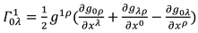
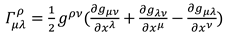
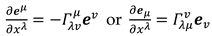
Christoffel symbols have been defined as

There is nothing wrong with the definition in that the derivative of a base must have a direction and so that to be written as a linear combination of the total bases. The key problem is what the Christoffel symbols are.
In this and following sections, all symbols of vectors and matrix would be bold written while their components and that of other quantities may be simplified written, no matter they are tensors or not.
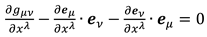
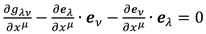
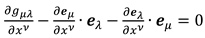
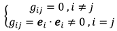
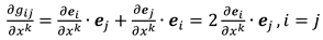
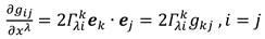
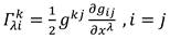
In most conditions, Christoffel symbols could be discussed by the derivation of metrics as

For the derivative forms with alternative indexes mathematically, there will be
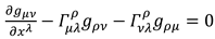
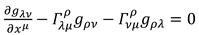
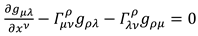
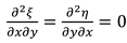
In the case that the so called torsions is set zero, the summation of the previous two equations minus to the last one that
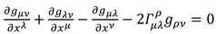
Generally, Eq. 49 - Eq. 51 could also be rewritten as the original forms
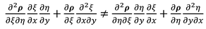
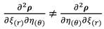
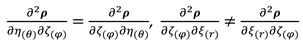
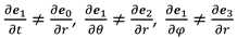
We will find that in some conditions the torsions do not always equal to zero. It is said that the mixed derivatives of bases and do not always equal, and then the Christoffel symbols with mixed subscripts and do not always equal, so that the Eq. (53) might be invalid in those conditions.
3.2. The Inequality of Christoffel Symbols of Mixed Subscripts
In differential geometry, the equality of Christoffel symbols of mixed subscripts is usually adopt the doctrine. But no forceful researches could provide reliable supports. The truth is that the problem of mixed derivatives of bases in a Riemannian space are far different from the problem of normal mixed derivatives of a 3-dimensional surface in Euclidean geometry.
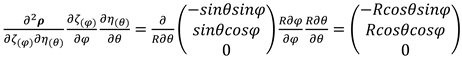
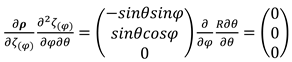
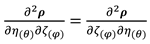
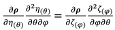
We could find out the truth that in the deduction of in Eq. (43), has been used instead of so that to gain . But we can easily calculate that and are not equal. We might have found out the problems.
3.2.1. Coordinate Transformations and Bases
Any points in a Riemannian space of Riemannian manifold of dimension has a neighborhood homeomorphic to a subset of Euclidean space of dimension , so that there must be probable maps between the neighborhoods and the corresponding subsets. It is just to say that the coordinates of any points in Riemannian space could be expressed with the coordinates of corresponding points of Euclidean space, and reversely. If a part or the entire of a Riemannian space are continuous and differentiable, Euclidean coordinate lines could be drawn in the part or the entire of the Riemannian space. On the other side, coordinate lines of Riemannian space could also be drawn in the corresponding Euclidean space. For convenience, the Riemannian space could be called covariant space, and the corresponding Euclidean space could be called contra variant space. A contra variant space is curved in the view of its covariant space, and the covariant space is also curved in the view of contra variant space.
It is obvious that transformations of spaces are actually coordinate transformations. These transformations could happen between covariant space and contra variant space, as well as they could happen among homeomorphic Riemannian spaces. Coordinate transformations may perform in the way with unequal metrics as well as the way with equal metrics.
The more effective method for coordinate transformation is to define bases and distances for spaces. Two examples would be presented firstly for definitions and for following discussions.
Example 1: Bases of Riemannian manifold of super surface
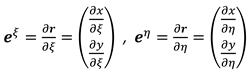
The derivative vectors of 3-dimensional surfaces were usually employed to form bases in classical differential geometry. The curve space has an extra dimension than a plane space that could be called the super surface. The Riemannian manifold of the super surface in the 3-dimensional space would have a homeomorphic Euclidean space in the space . The coordinate lines and in contra variant space could be transformed to be and in covariant space, while , and in covariant space be transformed to be , and in the space as shown in Figure 3 and Figure 4.
The super surface could be determined by a vector function

And the function could also be written as

or

At the same time, the contra variant space could be defined by

There will be varieties of available ways to develop the expressions of bases and distances. I prefer to put forward the followings might as well.
The way in super space:
In super space, the differential has 3 components

That of differential could be simplified to be 2 dimensional because it just locates in the space

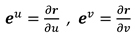
To define a set of covariant bases for a position in covariant space by
It should be pointed out that in some publications coordinate and vector symbols have been used reversely, which is just a kind of treatment, but in the theory of relativity they may bring about confusions.
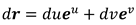
In covariant space, the differential expressed by with covariant bases
Differential distance could be defined as

If the bases are orthogonal, there is
We have seen that the covariant bases are defined in covariant space to help contra variant coordinates to form covariant distances.
There are more complexities for a transformation between a super surface in 3-dimensional space and that the 2 covariant bases would have 3 components
Define the contra variant bases for a point in the plane that
The 3 contra variant bases all have 2 components as
The differential expressed by in contra variant space
Of course, one can create transformation matrix to perform the relationship between and directly.
The distance could be defined as

If the bases are orthogonal

One could imagine that this condition you cannot give the relationship of metrics that equals to , in that the covariant bases have 3 components and contra variant bases have 2.
The way in tangent space:
Consequently, the issues could be simplified in tangent spaces. At a position in the covariant space, there is a neighborhood which will be labeled with coordinate lines of and , at the same time at the position , there is a corresponding neighborhood in contra variant space labeled with coordinate lines of and , as shown in Figure 5 and Figure 6. Generally, coordinate lines could be set orthogonal. In most of publications, and were seen as and , but one should realize that the difference really matters.
One could define the differential vector in covariant space

As a result, the bases
Again, there is the distance

The differential keep the form as Eq. (62), so that the contra variant bases could be defined as
Also, there is

In this case, the relationship of metrics go harmonized that equals to . It should be pointed out that the ways of expressions of bases are all equivalent except that the substitutions of coordinate lines and might have hidden some information of super surface, so that I would like to make analysis within super space in most cases.
Example 2: Bases of Riemannian manifold of equal dimension
As a Riemanian manifold has equal dimension with its contra variant space, it could be called equal dimension manifold. A plane space maps to a plane space could be taken for granted, as shown in Figure 7 and Figure 8.
A differential vector in covariant space is

The differential vector in contra variant space is

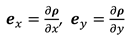
Thus, the definition of contra variant bases could be
To express with
Also, there is the definition of covariant bases
So that the expression of by should be
Something different is that a covariant base has 2 components
And a contra variant base also has 2 components

In the case that bases are orthogonal, the distance
 and
and

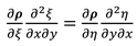
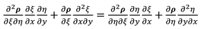
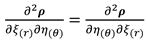
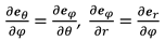
3.2.2. Inequalities of Mixed Derivatives of Bases
Now it is the time to carry out the first discussion on the inequality of mixed derivatives of bases. The mixed derivatives of bases are just special defined for bases alternative derivations. As transformation from contra variant space to covariant space is concerned, the covariant bases could be considered to be derivated by the coordinate lines in chain rule
 where, and are the direction derivatives along the coordinate lines and in covariant space, and and are their differential lengths in covariant space, which could be called the covariant lengths. And there will be a setting that Einstein summation convention does not act on double and double .
It should be pointed out that in most mathematics and physics, mixed derivatives being confirmed to be equal is because in the Eq. (88) and is incorrectly understood to be the differential length in covariant space , but they are really the lengths in contra variant space . That is the reason we have carried out the concept of covariant length and .
Thus, the mixed derivatives will be
 and
and
Consequently 3 conditions could be focused on:
Condition 1:
If there is an equality between the first items of the two equations that

For example, in the super surface, the mixed derivatives of course have the equality just as the equality of normal mixed derivatives of a 3-dimensional surface in a Euclidean space.
In this case and if there is another equality for the last items of the two equations that
Then that must come to the conclusion

Otherwise, that depends.
It should be pointed out that and do not equal in general conditions because they have different directions and in most cases they are usually set orthogonal, so that if that equality Eq. (92) happens, it asks for
We will see that in some cases it is really well satisfied.
Condition 2:
Most special if

that indicate the first items of the two equations are not equal, but at the same time if the total equations are still equal that
We will still obtain the equality that

Condition 3:
This is the condition after the previous two conditions and else to them. Generally if
No matter the first items of the two equations are equal or not, the mixed derivatives will perform inequality

Then, turn to the issue of geometrical influence that the inequality of mixed derivatives will cause closure errors [6,7]. I prefer to give a brief presentation. Consider a differential in a curve line coordinate system expressed by bases along different coordinate paths as shown in Figure 9 that in path 1,
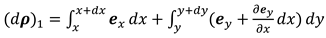
The irregular expressions of same symbols of integral variables and integral range could be adopted in special cases.
By Taylor’s approximation, it could be written as

We could also get the differential in path 2,

Trimming off the 3-order infinite small quantities, the difference of and is
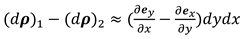
There will be a closure error in close path if the mixed derivatives of bases do not equal.
3.2.3. Verifications and Discussions
Example 1: Polar coordinate system
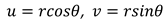
Polar coordinate system that we are familiar with is a transformation from its contra variant space , as shown in Figure 10 and Figure 11.
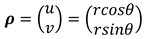
A position in contra variant space could be expressed by vector

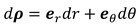
and the differential is

Corresponding position in covariant space, will be expressed by

and the differential is

In the contra variant space, the differential distance between two positions could be defined as
The system we have used to is the one that has experienced transformation from space with
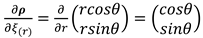
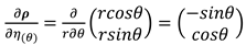
The bases
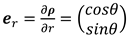
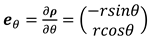
so that
Thus, there is the covariant distance

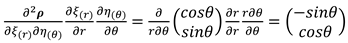
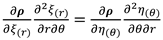
The mixed derivatives of bases
We have seen the mixed derivatives got equal

It could also be verified in Eq. (89) and Eq. (90) that
and
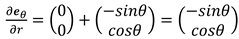
The vector is
Because is radius length , and is arc length , then
Thus, the first item of Eq. (117) is
The second item is
And the first item of Eq. (118)
The second item
so that
and
Obviously there is
and
and then

Again, we have got the equality of mixed derivatives. But to our surprise is that this solution really subject to condition 2. It is said that the first items of Eq. (117) and Eq. (118) do not equal. One of the reasons in this case, is that there is no super surface.
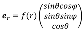
Example 2: Spherical surface coordinate system
A spherical surface coordinate system is also a transformation of the corresponding contra variant space as in Figure 12 and Figure 13, in which
Differential distance is
And the coordinates of covariant space will be expressed with
The spherical coordinates could be transformed to Cartesian coordinates,

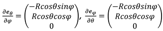
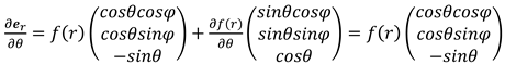
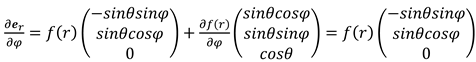
The bases could be defined as
and
Thus, there is the covariant distance

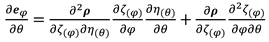
The derivatives
so that

It could also be verified in Eq. (89) and Eq. (90) that
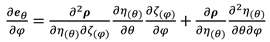
and
The vector is
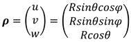
Because is arc length , and is arc length , then
Thus, the first item of Eq. (140) is
The second item is
And the first item of Eq. (141)
The second item
With Eq. (145) to Eq. (148) we found that
and
so that there is

One can see that this is of condition 1.
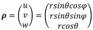
Example 3: Spherical coordinate system
A spherical coordinate system is also a transformation of the corresponding contra variant space as in Figure 14 and Figure 15, in which
Differential distance is
And the coordinates of covariant space will be expressed with
The spherical coordinates could be transformed to Cartesian coordinates,

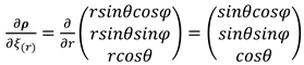
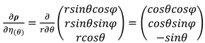
The bases could be defined as
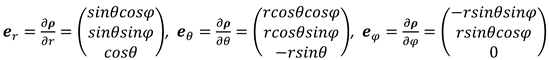
and
Thus, there is the covariant distance

The derivatives
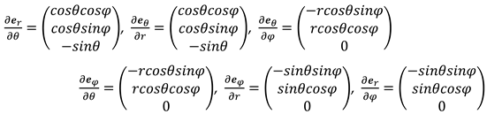
so that
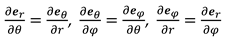
It could also be verified in Eq. (89) and Eq. (90) that
and
The vector is
Because is radius length , is arc length , and is arc length , then
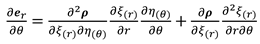
Thus, the first item of Eq. (161) is
The second item is
And the first item of Eq. (162)
The second item
With Eq. (167) and Eq. (170) we found that
but there is

One can also calculate that
At the end we can obtain
One can see that one of them is of condition 1 and the others of them are of condition 2.
Additional discussion: deformed bases of example 3
If one of the bases in example 3 be set deformed as
where, is a function of coordinate .
One will find that the derivatives
and
 while and will still keep the results as in Eq. (159), that will cause

This result reminds us that the same performance would have happened in gravitational space time that will be put into discussions in next section.
4. Metrics and Covariant Derivatives in Space Time
4.1. Metrics in Pseudo Riemannian Space
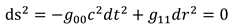
Pseudo Riemannian space is raised for the description of space time for general relativity, after Minkowski space for special relativity [8,9]. For Minkowski space, invariant distance for flat space time could be written as
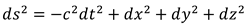
We know that there is a minus signal in the equation. The minus signal does not come from transformations of spaces or coordinates. It is a kind of mathematics and physics setting. Former researchers have made efforts on this topic, for example, the concept of plural employed to reform the base [6]. But plural bases for relativity is not a good idea. Another treatment is to define , which looks like more reasonable [7]. The more important is that the metrics for this condition should be carefully treated so that the metric will not be minus.
In general relativity, spherical coordinates are usually suggested for one source problem. So that there will be contra variant space and covariant space . The invariant distance of Schwarzschild solution is

So that there could be a brief expression of invariant distance
As we have discussed, that will cause plural bases. Anyway, minus metrics is improper. In fact, it is one of the reasons that cause the wrong result of acceleration calculation in Eq. (43).
Considering the above discussions, I prefer to give the invariant distance of one source field as

Thus, we will prevent from plural items. That doesn’t hurt the expressions of relativity. Metrics and bases defined are just employed for the transformation from Minkowski space time to pseudo Riemannian space time. Even if one persists the coordinate the invariant distance will still keep the expression. Additionally, I still suggest in use that will bring about convenience in most cases.
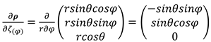
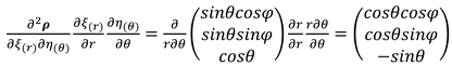
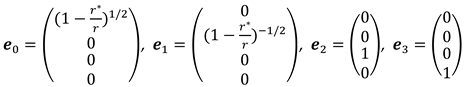
It should be highlighted that the bases still would have sophisticated forms that
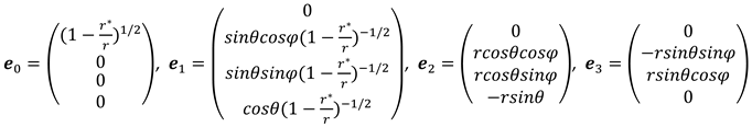
That is because the spherical space we have discussed has already experienced coordinates transformations. The transformed coordinates are not real spherical coordinates, they are the Cartesian coordinates expressed by parameters of , which could be called parameterized Cartesian coordinates. One can learn from previous section for the reasons.
It could be calculated that
there are
In general relativity, it could be suggested to simplify the presentation that we only focus on the gravitational transformation. So that the contra variant space is no longer of real spherical coordinates, which could be set as parameterized Cartesian coordinates, and the covariant space could also be the form of parameterized Cartesian. Thus, the invariant distance could be expressed as

In which, .
These metrics could be called the gravitational metrics, while the metrics previous could be called total metrics and the metrics before gravitational transformation could be called original metrics or spherical transformation metrics.
For gravitational metrics of Schwarzschild solution, we have the bases
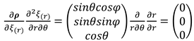
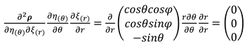
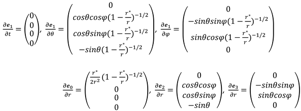
It could be calculated that
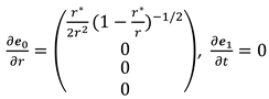
so that

This is of the condition 3 that we have discussed in section 3.2.2. One can also calculate the inequality of mixed derivatives of bases of total metrics.
That reminds us that the inequality of mixed derivatives of bases will cause closure errors in space time, which would be left for more discussions elsewhere.
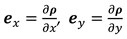
4.2. Discussions on Bases, Tensors and Their Derivatives
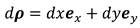
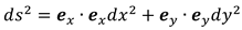
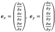
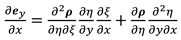
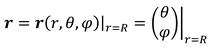
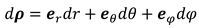
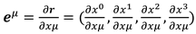
Tensors could be recognized as the quantities relating to coordinates in space time. Case a tensor varies in space time, the variation rate could be inspected by derivation. The simplest tensor is position vector . You have seen that we are going to use middle subscriptions to express coordinates and tensors in covariant space time, though they are rarely mentioned in most of references. To study its variation in space time, one could define the distance variation ratio to form the bases

For any tensors involved with bases, such as a proper tensor

where, is number component of the total contra variant tensor.
The derivatives of the tensor are
The differential of a proper tensor could be defined to be covariant differential labeled as , and then the derivative to be covariant derivative
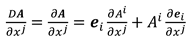
In these equations, the middle subscriptions of proper tensors maybe neglected conventionally so that it is expressed as . And the tensor could be called proper tensor because has already been named covariant tensor conventionally. Because or is just a component, we could imagine that there must be the total quantity. That will be expressed to be or for convenience.
Bases sometimes look like one-order tensors since they have a single index in expressions. But in fact, they really are two-order mixed tensors. For example, a component of contra variant base of collinear transformation,i.e. coordinate lines of contra variant space and covariant space coinciding, could be written as

where the contra variant base and proper coordinate differential are all labeled with middle index .
So that the base really is

If =0 with , we could use instead of for convenience, as it is the only nonvanishing component.
For any one order tensors there is a transformation
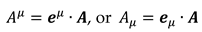
But for two order tensors, there are some things different. For example, a component of contra variant velocity could be transformed from proper velocity
We know that it may be seen as one-order tensor in practice, but it is really two order tensor.
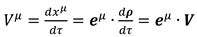
As for velocity totally in contra variant space as , that would not be worked out by direct vector product.
In fact, it could be composed independently by and .
It is impossible to get from and the latter is zero. Notwithstanding, a velocity is a derivative on matter’s trajectory rather than a direct derivative. That will be further discussed in next sections.
4.3. Derivation via Christoffel Symbols
Christoffel symbols were put forward to perform geometrical relationship that takes similar effects with that of bases. They are defined in the equations [3,13]
Taking the first one for example, the purpose of the equation is to consider the derivatives to be a function of bases, so that the right hand item is really a kind of trivial types. In the summation items, just act as direction indicators that would give out whole basic vectors of entire dimensions. And then, provide the coefficients of all directions. It is said, this definition has just provided an error-free frame for the functions of derivatives. It means there may be redundant designs for the coefficients.
Since there is probability of inequality of mixed derivatives of bases, we should define a specific sequence for subscripts of Christoffel symbols. For the traditional reasons, will be defined as the coefficient of a derivative of that is derivated by , on a direction of ,that requires unexchangeable subscripts of .
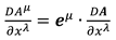
We know that a covariant differential is exactly a differential of a proper tensor

This highlightable concept is essentially carried out to perform general covariance.
The contra variant form also performs the same covariance as that
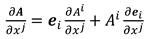
You might have found that the tensor component has been expressed by a total tensor is exactly partial expression. It is just of traditional operations. One can of course carry out whole form expression of expressed by with base matrix . But too more renovations in a performance will bring about more reading difficulties. So I prefer to present equations in traditional forms as far as possible.
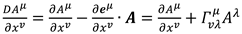
A component of contra variant tensor transformed from covariant one

Its derivatives is

so that
It is easy to study those covariant derivatives for covariant tensors
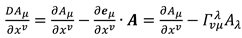
We have seen that the methodologies of Christoffel symbols and the derivation directly from bases are actually equivalent treatments that present the covariant derivatives. That of course may be use to inspect the problems of equations of Christoffel symbols. Since we have known that part of Christoffel symbols with mixed subscripts do not equal in space time, it is necessary to do more discussions.
It is convenient to discuss the case that a space is defined by orthogonal bases. In practice, metrics are usually taken in to Christoffel connections analysis. For a series of bases , there is the metric

For whole orthogonal coordinate spaces,
The nonvanishing derivatives
Then the equation could have nonvanishing value, that
Then
This equation could be called revised equation for Christoffel symbols in general relativity. In the equation, it also need for the to get nonvanishing.
For a result, this equation could be verified in a covariant derivative directly as that in Eq. (206) that

It should be pointed out that the Christoffel symbols are not necessary because that the issue only started from derivatives of bases, as consequences they surely might be taken the place by the operations of bases.
4.4. Derivatives on Matter’s Trajectory
The calculation of time derivatives may cause to another mathematical abuse in classical theory. For a one source field, it could be seen as rest field in general. Thus, a time derivative of a field quantity should be zero. Case a matter moves in a space, it is the issue that the matter changes its position in a time interval and forms a motion trajectory. In this condition, to learn the acceleration is to study the position variation rather than field variation. It is one of the reasons that make errors in covariant derivative calculation in Eq. (43), in that the direct derivative has been used instead of trajectory derivative.
It is valuable to reclassify tensors to be field tensors and motion tensors, thus field tensors may vary with field while motion tensors should vary both with field and matter’s motion. For example, the bases only depend on gravitational field, while velocity of a matter may vary due to positions changed. For example, case in one source field, a space derivative of a base may be nonvanishing, but a time derivative of a base must be zero, nevertheless, the base relating to a matter moving in space time would vary because the coordinates varied on trajectory.
A trajectory of motions of a matter should be a directed curve line in a space, from the start to the end. It is said that the trajectory must be single parametrical curve line. Theoretically, the parameter maybe natural i.e. the line it pass through, and as same it could be time that the motion experienced. What worthy of highlight is that these parameters are simultaneous. That is said a record of the parameter corresponds to a sole record of another. The parameter indicates the sequences.
It is no harm to discuss the trajectory vector as a curve line in contra variant space, in that the trajectory is a function of single variable. There is
 where is the length of trajectory.
It is said that the trajectory is of

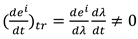
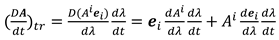
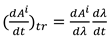
A tensor variation ratio during a time interval on trajectory could be defined to be trajectory derivative that
For example
where, Einstein summation convention does not act on double because trajectory is just a single line. The differential length d is the differential of matter’s trajectory, so that is the covariant differential of tensor between two neighbourhood positions on the trajectory. Thus, the so called trajectory derivative is really a kind of line derivative that is derivated by a parameter.
It should be noted that there is the substantial difference between trajectory derivatives and original derivatives. A differential on trajectory is the distance interval that a matter has past across, so that the velocity is a trajectory derivative
As mentioned above, bases are defined by direct derivatives such as
where, is a proper coordinate differential, so that it is middle labeled.
For the velocity, the differential is exactly defined on a trajectory of a matter, so that there is the probability that

It is said that velocity tensor itself is literally trajectory derivatives.
Trajectory derivatives of general tensor should be labeled for discrepancy.
For example, the bases along a trajectory in rest field
while direct derivatives with

Eq. (216) could be calculated as
and is also time derivative, and there is
where, Einstein summation convention does not act on double .
Thus, we have seen the difference between a trajectory derivative and an original derivative.
On the other hand, the value of matter’s velocity

so that
 where, Einstein summation convention does not act on double , and is the direction cosine on the direction of vector line , so that is of component of on that direction and is vector form of so that it could also be written as equivalently in this equation specially for matter’s motion on the trajectory.
It could be expanded to be
The expression in component forms could also be worked out as

The expression in the way of Christoffel symbols as

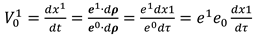
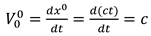
We could find that the first component of 4-dimensional velocity is something special in that it is not true velocity. Generally, a velocity of massive matters in contra variant space is
And velocity composition expressed as
 where .
For light rays, the contra variant velocity will be composed to be nonvanishing
 where .
But their velocity composition in covariant space is zero

in that the summation of the last 3 items is .
We know that invariant light speed is . It is said that the composite velocity does not perform real velocity, so does the contra variant composite velocity. The velocity of or is something virtual quantity, and we have found more complexities in kinematics. One can argue that there are still some issues unsolved. That could be expected in next sections.
In rest fields, there is , so I prefer to suggest the real trajectory derivatives of rest field for discussion that

and

It should be highlighted that the trajectory derivatives could also be defined in distance derivatives as
which just performs a special appearance of trajectory derivatives.
For free falling trajectory, it is
Trajectory derivative is derivative on a curve line in space time. Sometimes it is presented with time because that the time variable is used in the parametric equation. Christoffel symbols in the equations owe to derivatives of space differentials rather than time differentials. We will see that the concept of trajectory derivative help to describe frequency shift and acceleration, as well as to falsify the concept of geodesic line in Section 8.2.
5. Theoretical Verifications on Gravitational Redshifts and Accelerations
Because of the inequality of mixed subscripts of Christoffel symbols, the classical Christoffel symbol equations could not be used any more in the theory of general relativity. The covariant derivatives in gravitational field should be considered in their correct forms.
5.1. On Gravitational Redshifts
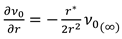
Light rays travelling in gravitational field, are also the issue of matter’s motions. Something special is that we would rather focus more on the frequency derivatives by distance, in that they perform more details of the concept of redshift.
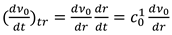
Taking light propagation at vertical direction for example, a distance derivative of contra variant frequency is exactly trajectory derivative
It is sure to consider the tensor of frequency and its derivative to be vectors, but in traditions it is not of a rare necessity. It has been mentioned that Christoffel symbol were employed correctly with the form as has been shown in Eq. (26). As a result, it will lead to a real answer

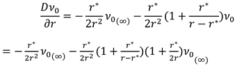
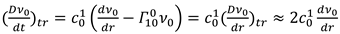
The covariant derivative will be calculated to be
The approximate solution for weak field is that
It is said that the solution Eq. (28) is confirmed again, and in weak field that reveals the covariant redshift is approximately double of the contra variant one.
Notwithstanding, one can also make another derivative as
For light rays, . It becomes
The first item of right hand side can also be transformed to be
so that
5.2. On Accelerations
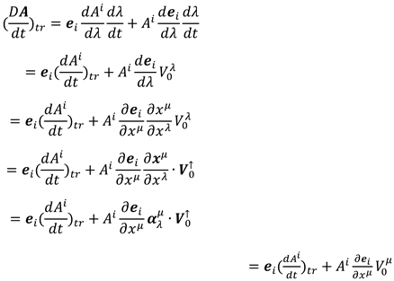
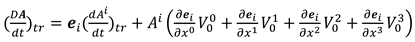
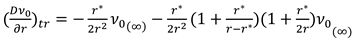
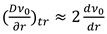
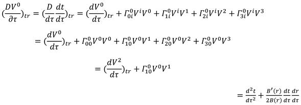
One can take matter’s freefalling for example to study the acceleration in gravitational fields. The entire contra variant acceleration is the derivative of contra variant velocity as that

And entire covariant acceleration is a pure covariant derivative
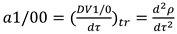
One may find that some tensors have been labeled with detailed middle index hence they may help to provide explicit expressions, in which / is employed to divide middle upper and middle lower indexes.
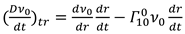
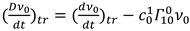
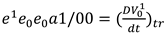
With the relationship between covariant derivatives, it is drawn that
To study the covariant derivatives in the way of Christoffel symbols, there is
With , it becomes
With , , and there is
With Eq. (247), there is

One can find that we have use and in the calculation of , rather than that has been used in Eq. (44). As we have discussed, the value of is really of zero.
As has been said that covariant derivatives could also be developed in a direct way without Christoffel symbols
It could be found that this equation has been far different from the Eq. (44), because errors in Christoffel symbol equation have been eliminated and at the same time the concept of trajectory derivate help to calculate an acceleration in right way. These discussions have presented further verifications for the revised equation of Christoffel symbols of Eq. (211).
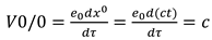
By the way, it is interesting to take some discussions on some trivial concepts such as and the covariant form of massive matters. Since and are the velocities of contra variant time and proper time but not the real velocity of light
and
Then their derivatives are just the accelerations of time coordinates that
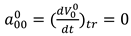
while
so that

As light propagation at a direction of a radius is concerned, we know that light speed keeps invariant in covariant space, so that there is

Case discussing the performance of contra variant light speed, with invariant distance, there is
and then the light speed in contra variant space will be
where, positive is set instead of a minus as has suggested previous.
Then the acceleration

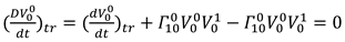
With Eq. (250) the covariant derivative is
Of course, with Eq. (260) and Eq. (247), we could obtain the result only by a judgment that
6. Experimental Verifications on Gravitational Redshifts and Accelerations
Every tensor involved with measurable quantities could have probabilities to be performed in practice with measured quantities to verify their theoretical expressions. In space time, space intervals and time intervals are all measurable quantities so that they surely could be employed to perform the space and time dependent tensors.
The methodology of the so called revisit gravitational redshift encourages me to sponsor a realistic analysis method to further verify the general covariance, which will present solutions all based on physical events of realities. Physical events always have substantial existence so that they can help to create irrefutable conclusions. We know that physical events may be record both in contra variant space and covariant space that might provide different values for physical quantities, but both of them actually represent the same physical realities.
6.1. On Measurable Experiments
Measurable quantities could be used to describe physical events, which may be coordinate independent or not. Coordinate independent quantities of course show invariance in physical events in different spaces, such as wave numbers, which could be record as images or texts at specific times and positions. However, coordinate dependent quantities measured in site maybe really dependent. For examples, distance measurements not only depend on in-site space intervals but also depend on the in-site rulers, so as well, time measurements also depend on both in-site time intervals and the in-site clocks. We imagine that the space rulers and clocks their selves maybe also vary. Logically, records of these quantities are recognizable even if they are in farthest distance to the bystanders.
Case a measurement equipment varies with time space, whether the measurement quantity measured is in contra variant space quantity or covariant space quantity? With general covariance, it has been believed that rulers will shrink when they go closer to the center source corresponding to the space interval to become shorter. And also, it has been expected that clocks will go variant corresponding to their dynamic conditions.
However, after those inspections in previous sections, we know that general covariance does not work in some circumstances. Energy and momentum of a matter may not keep covariant in covariant space, while light speed may keep covariant spectacularly. On another side, our discussions may have led to a theoretical inference that matters may experience relativistic emission when they go to a center source and then shrink because of the variation of energy structure. That could be called covariant deformations.
Once we measure space and time intervals at a position, maybe they are not committed to be contra variant quantities or covariant quantities, because our rulers may vary uncommitted. But we could do made measurements anyway. In another word, we could indeed measure something so that they will correspond to any others. Thus, it is not harmful to suppose one of the series of measurable quantities could be measured in following discussions, for example, the contra variant distances or contra variant time intervals. And then they will be valid to be transformed from one to another. That will help us to do more analysis for comparisons and discussions.
6.2. Measurable Verifications for Gravitational Redshift
For the issue of redshift, we are going to sponsor the physical events of wave number counting. It is known that light frequency investigation should be accomplished by indirect techniques and sometimes it may come out with deviations. But it is supposed here that the wave number of the light is countable, or it is believed that light wave could be seen and record. This assumption actually may not do harm to our understanding to the realities, because it indeed will not change the realities and the events of wave counting in that the measurements themselves are also physical processes.
The event of wave number counting could be specified as the record of a number of waves to past a position in a time interval, and it could also be simplified to be one wave corresponding to a time lasting of the light ray propagating a wave length distance. On another side indirectly, one can get wave number by measuring wave length, based on the assumption of invariant light speed. But the apparent light speed might be variable so that the indirect method is not a good idea.
If there is a photon propagating from position 1 to position 2 in a one source field as shown in Figure 16, which correspond to coordinates and ,
The wave number counting events should be carried out at the time that the photon passes the position 1 and position 2. In very short time and , we will count the corresponding wave number and .
Since the frequencies should be calculated as
Redshift has been defined as
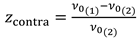
With the measurable records, redshift in contra variant space is
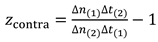
In the event of wave counting, wave numbers are invariant in both contra variant space and covariant space, but the time intervals and will vary to be and . In fact, every physical event keeps the only one event, whereas the different describing metrics lead to different results in the different spaces.
Naturally, gravitational redshift in covariant space is
 where, this redshift symbol labeled with revisit is because it corresponds to that one named in classical equations.
As we know,

It turns to be
As in a field of center source, the metric takes the forms of Schwarzschild solution, it is drawn that
We know that the in Eq. (266) could have been measured in the physical event of wave number counting that of course equals to that in Eq. (9), so that
Thus, the covariant redshift in weak field is obtained

It is said that, the revisit gravitational redshift is double of that of contra variant one.
As the equation of contra variant redshift is concerned, we know that it could be of course drawn by counting two wave numbers in two equivalent specified time intervals. For example, set which are measured at positions of and , then and should represent the difference of frequency without time intervals. So that
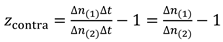
We know that and present the wave numbers with respect to and .
As for revisit redshift, one will still get different covariant time intervals because the metrics go varied. Thus it is again doubled of the previous.
It should be pointed out that in some experiments on gravitational redshift, only one timing clock was designed for time interval measurement. In this case, a wrong setting of proper time intervals may be taken into consideration, so that the experimental redshift may be presented as
 where, is base component at clock position of or or any position other to them.
We can find out those completed experiments observations [14,15,16] on gravitational redshift will be easy to be verified to have only worked out the results of contra variant frequency shift.
Of course, one can calculate the real proper time intervals by time interval transformation between sole timing position and frequency shift positions. That will still help to work out revisit gravitational redshift as have discussed.
6.3. Measurable Verifications for Acceleration
6.3.1. Measurable Quantities and Measurable Acceleration
Firstly, I prefer to rise a controversy of a free falling on the Earth that if a matter freefalls from rest with velocity as well as by nature, we do know that it will move quite faster with velocity after traveling a distance and a time interval because of gravity. In traditional theory, we know that the proper velocity . Considering the weak field effect, there is . Hence comes the controversy that the covariant acceleration must be great than zero because the matter has started from rest to a quite apparent motion. That is really contradicted with the principle of general covariance with a requirement of zero covariant acceleration. Nevertheless, considering that and are still non-relativistic velocities, it is easy to estimated that the accelerations are also approximately equal that . The following works of so called realistic verifications in this section are exactly to be sponsored to solve these controversies thoroughly.
One cannot count on an investigation only by measuring a distance and a time interval of a freefalling to get a contra variant acceleration and then transforming to proper one to discover the difference. It is because that a distance a matter flies across in a time interval, does not interpret accurate velocity variance but gives a mean velocity.
Then we know that it is difficult to measure acceleration only at a single position, so that I would rather sponsor an investigation based on two-position measurements. A freefalling test with initial velocity is going to be put forward, in which a matter freely falls to source center from a position to a position shown as Figure 17. Once the velocities at the two positions are measured, the average values could be estimated with the velocities difference and the interval distance. Considering the condition on the surface of the Earth, a freefalling with a rarely big velocity and a rarely small travel would be performed. For example, a velocity of more than 10000 m/s, could be seen as a constant accelerated motion even in covariant space, in that a covariant derivative is expected to be linear with velocity.
It is supposed that contra variant distances and time intervals are measurable. Based on the measurements, velocity at position 1 could be written as
 where the and are measured distance and time intervals when the matter goes by the position , so that they are both tensors of contra variant space. For reasons of convenience their bracket sub indexes here are only employed to represent positions.
As well as that at position 2

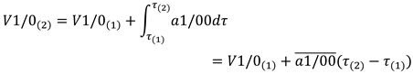
Because the velocity at position 2 is the result of acceleration, it could be written in integral form
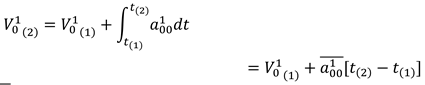
where, the mean acceleration is the integral point value, and is time interval for the matter traveling from to .
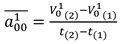
So that the mean acceleration is
On the other hand, with covariant bases there are the relationships of contra variant quantities and proper ones

One can use the mean metric to calculate the proper time intervals from position 1 to positon 2
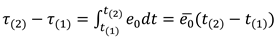 where the is the value at integral point, and it is suggested to be evaluated approximately as following in weak field
The proper velocities
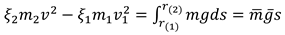
And the integral relationship in covariant space that
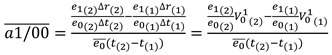
And also, we get the mean covariant acceleration with Lagranian mean value theorem of integration that

So that the mean covariant derivative
It is of course the measuring forms of an acceleration of a freefalling. And then it could be compared to that of contra variant one.
We would like substitute the equation of contra variant velocity 2 of Eq. (278) into this equation. That is
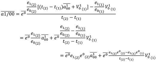
It could be transformed to be
Here we have got the transformed form of covariant acceleration of freefalling.
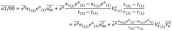
Nevertheless, with Lagrangian differential mean value theorem, we can write down the differential form as
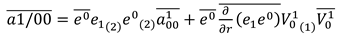
Or the form of reverse bases

Thus by the way, another kind of proof of differential analysis of the Eq. (252) and Eq. (249) has been completed, in the way of measurable experiment.
6.3.2. Examples
Some terrestrial experiments are going to be put forward, that matters with initial velocity freefall in vacuum circumstance with in 1000m height to the ground. Both at the start point position 1 and end point position 2, the matter’s velocities will be measured. And of course, the space and time intervals between position 1 and 2 that depend on the so called geodesic line will be measured together so that to calculate the mean accelerations.
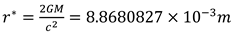
Some basic data of the Earth have already been tested certainly, so that we can take the standard value for our experiments, such as the total mass of the Earth , and the position on the ground could be assigned to have a radial coordinate . We could also take the gravitational constant , with the light speed thus the gravitational radius will be calculated as
With Newtonian equation and Schwarzschild’s solution, some positional data could be list in following Table 1.
So far as we have discussed, the accelerations and are really geological quantities, and now it is necessary to make an extending study. We know that all kinds of interactions could be seen as momentum exchanges between matters, as that
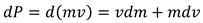
For the convenience, some quantities discussed in this section will not be marked with tensor index anymore.
In conditions of low velocity motions, the theory of special relativity indicates small mass variations, thus

For the cases of high velocity motions, one should take a total analysis. Now the total acceleration could be defined
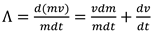
It is said, the total acceleration includes mass variant acceleration and velocity variant acceleration, and the latter also could be called geometrical acceleration.
With a momentum variation, kinetic energy will vary a difference
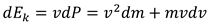
At the same time, the mass energy equation of differential form is

Thus, there will be
To be divided by time differential, there is geometrical acceleration
Now one can define a coefficient of geometrical acceleration
In one source field, single acting gravitational geometrical acceleration is
 where is the total acceleration of gravity.
We will see that geometrical acceleration declines as velocity goes up to a relativistic level, and it goes to zero as velocity closely catches up to light speed.
If a matter is accelerated from rest, the total energy includes rest part and kinetic part
 where is relativistic mass and is rest mass.
We know that in special relativity there is

Back to Eq. (302), there is
Then the total kinetic energy
Case is a small value, would be close to 0.5, so that

On the occasion of freefalling the variation of kinetic energy
Again with Eq. (298) the energy difference in an experiment
Thus, there is
Considering in experiments, the difference of kinetic energy could be written as
so that
Thus,
Unfortunately, this solution cannot come up with a higher accuracy than that

After then, we are going to sponsor series of freefalling experiments. Contra variant accelerations and covariant accelerations for every position are easy to calculate. While measurable covariant acceleration could be obtained with measured distances and time intervals via Eq. (287). But it is convenient to calculate with Eq. (289), in that the latter is just a transformation of the previous. And in this equation, space intervals would be gained with Newtonian equations and time intervals with Eq. (313) for convenience. One may argue that the measured quantities might come from calculation. That doesn’t matter, because the equation has been verified for hundreds of years, therefore it is sure that the calculated quantities have equal value with that by measuring. And then the mean covariant acceleration will be taken to compare with the contra variant acceleration calculated with Eq. (301) and covariant acceleration calculated with Eq. (249) or Eq. (252). Calculation results have been listed in Table 2 and Table 3.
7. Conclusions and Inferences and Their Applications
7.1. Conclusions
Previous discussions will lead to two conclusions for matters’ motions in gravitational fields:
1) For light: Light speed keeps general covariance, but light frequency keeps conservation in contra variant space.
2) For massive matters: Massive matter’s velocity does not perform general covariance.
These two conclusions have been drawn based on three items, which are light speed invariance, gravitational redshift measurement and acceleration measurement. Among these items, light speed invariance is a theoretical setting. This setting is come from special relativity and observational verifications. Gravitational redshifts and accelerations could be measured in realistic events that guarantees the conclusions in a very high reliability.
It is only the general covariance of light speed that has been observed. That relates to the inacceleratablity of light rays even in contra variant space, which is one of the performances of light speed invariance.
7.2. Inferences
These conclusions are really different from classical theory of general relativity and they will then lead to natural inferences. I prefer to focus on the inferences on kinematics and relativistic release:
1) For kinematics: General covariance goes break by a large range. During the motions in gravitational field, all matters, including light rays, will keep energy and momentum conservation in contra variant space rather than that in covariant space. Only for light rays they may keep velocity invariant in covariant space, but their energy and momentum will still keep conservation in contra variant space. Energy momentum conservation is the conservation under the condition of gravitational potential conversions. It is said that there is only one exception in realities, the light speed invariance, which will lead to the validity of light ray propagation Lagrangian. While for massive matters, Lagrangian goes invalid. In any positions in gravity fields, massive matters always have opportunities to be accelerated up to and keep velocities close to absolute-light-speed.
2) For relativistic release: Since apparent light speed may vary in gravitational field, that will bring changes to interaction ratio in particles of massive matters to influence fine structures. For electromagnet force there will be of variation of momentum exchange. It is also reasonable to predict that the speed of gluons relating to the strong interactions is general covariant like that of photons. On the other side, these interactions keep energy momentum conservations at the same time. Therefore, case massive matters inflow enough intervals in gravitational fields, they might get an excited state and release, which could be called relativistic release, just as excited electrons might do. The difference is that relativistic releases may experience thoroughly exciting in whole intrinsic structures, including exciting of electrons. Matters may also experience covariant deformation after relativistic release because of equivalent state.
7.3. Applications
Detailed discussions on some applications will be sponsored consequently that will greatly support the conclusions and inferences.
1) On kinematics: General covariance and conservation principle are the two key handles to rectify the classical equations, especially the principle of mass energy conservation. It would be seen that those efforts to employ the geodesic equation or covariant derivatives to build kinetic equations have already gone failed, in that covariant derivatives may be actually nonvanishing.
2) On relativistic release: The concept of equivalent state would be carried out to estimate the energy exceeding for inflow matters so that to discuss energy release, which will then lead to relativistic redshift of emission and absorption. Equivalent state also relates to relativistic deformation that might perform another kind of covariance.
8. Kinematics and Dynamics
8.1. The Most Important
The second Newtonian law interprets the mechanism of accelerative motions of massive matters so that to form the dynamics. Case in the conditions that matters have relativistic velocities, forces acting on matters will cause not only the variations of velocities but also the variations of matter’s mass. It should be pointed out that a force really is of a statistic quantity rather than an essential physical quantity. In fact, a force is just a performance of exchange of momentum, as well as mass energy. Thus, that physics could be called the relativistic dynamics.
But for light propagations, the second Newtonian law will not take effects anymore. Even in the case that a force is vertical to a light ray, we will see that the second Newtonian law remains invalid. That is the reason we suggest the concept of kinematics that others to the concept of dynamics. If we persistently employ the concept of dynamics, it should be a new one.
No matter the space time been determined by what kind of metrics and labeled by what kind of coordinates, it is just a methodology for descriptions for physical events. None of them would have priorities. Physics is on earth depends on its nature rather on spaces. The most important is the conservation principles in realities.
It is easy to imagine that geodesic line could be employed for the solution of kinematic trajectories of matters, because general relativity expects conservations in curve space. But we will find out that geodesic equation or covariant derivatives have not really taken effect in the solving of the kinematics in the past century. We know the reason is that covariant derivatives may be nonvanishing so that those imposed settings of vanishing covariant derivatives might cause discrepancies to realities.
Most of methodologies for kinematic trajectories published were based on the so called Lagrangian. Besides these conditions, contra variant angular momentum conservation has been used in all of those solutions. One can imagine that this condition is apparently contradicted with general covariance. In fact, it is always the greatest reason for me to persist in this issue with more efforts.
Finally, the Lorentz covariance is also a kind of constraint condition, since it has been involved in the settings of Minkowski space and pseudo Riemannian space.
8.2. Discussions on Geodesic Equation
The geodesic line equations presented by Weinberg [17] with metrics given by

is
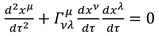

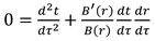
And then, with , the so called kinematic equation, were finally drawn as
 where, and are set constants.
It seems that the kinematic equation has been created by covariant derivatives. But it should be pointed out that Eq. (315) to Eq. (320) have gone wrong. Because we have discussed that the covariant derivatives could be nonvanishing in some occasions, so that there must be something wrong involved.
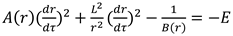
We are going to sponsor investigations in two ways for a comparison. Firstly, a transformation from the tangent space defined as to that defined as will be put into considerations.
The Eq. (228) could by employed for the solution, so that the derivative components could be performed with and then

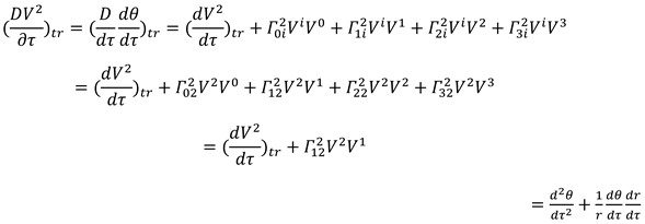
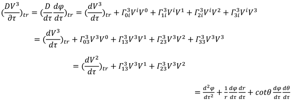
 where, is number component of contra variant velocity.
We have seen that some errors in the Eq. (316) to Eq. (320) have been rectified. In fact, it is easy to find out calculation errors. If any the Christoffel symbol of =0, in that the bases we discussed are orthogonal.
Secondly, we are going to study another condition that the tangent spaces from to . The invariant distance could be written as

(325)
One may argue that this transformation has overcome Riemannian manifold definition because the contra variant space is not a . But on earth in mathematics, that doesn’t matter because we know that the space could map to a at all. The derivation regulars are still available. Then the derivatives should be performed with Eq. (228) that
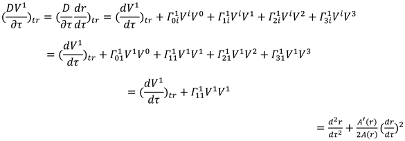
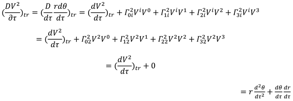
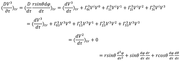
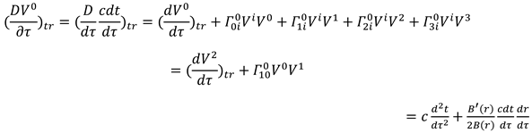
In comparisons of the last two calculations, we could find subtle nuance in that they are settled by different and . But they have really given the equivalent results, in that both of them could be transformed to uniform covariant derivatives . Because the latter calculation is very easy to be done, it is also a kind of verification to the previous. And moreover, the most important, the comparison calculations have verified the conclusions on inequality of mixed subscript Christoffel symbols, because the last result is easily worked out and approved to be right, and then one could find that the simplified expression of the second step could be used to verified the solution of the first step. That will finally indicate the errors in classical theory, as well as that in Weinberg’s calculations on geodesic equations.
We know many efforts [11,12,17] have been made to attempt to prove the conservation principles after the equation of geodesic equations that it is expected
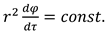
come from the Eq. (318), and
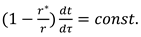
come from the Eq. (319).
It is easy to find that all of the works involve with errors. In comparison on the results of and in previous two kinds of strategies, we will find that the two derivatives do nothing with gravity influence, and they are just come from transformation of spherical coordinates so that any doctrines after that to form angular momentum conservation principle would be lack of supports. We will make further verifications in next sections that these two equations are all false. In fact, the Eq. (330) is not a correct form of angular momentum, and the Eq. (331) does nothing with energy. We will see that, motion trajectories cannot be calculated based on covariant derivatives, in that they are really not the geodesic lines.
8.3. Classical Equations of Light Ray Deflection
It is indicated in some books that Lagrangian relates to Euler-Lagrangian equation and geodesic equation [3,4]. It is trivial to continue the discussions on whatever of the origins. I will say that the Lagrangian equation for light rays is absolutely correct, because we will see that it is just the expression of composition of light speed components in covariant space. It is the reason that the Lagrangian is employed for the equation of matter’s trajectories in most publications. In fact, velocity composition equation could be easily employed to solve the trajectory of Newtonian problems. But it should be pointed out that the Lagrangian equation is not proper for massive matters, which will be presented in following discussions.
Incomprehensibly, classical solving processes for Lagrangian equations seem like to do nothing with geodesic line equation and covariant differentials. On the other side, we could find that those solved trajectories all involved with contra variant angular momentum conservation, which indicates that the solved trajectories may be not real geodesic lines.
To take the problem of the light rays passing across the Sun for granted, as shown in Figure 18.
It is expected in classical theories that for the motion of light rays, the Lagrangian is zero
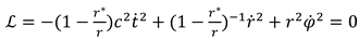
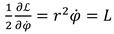
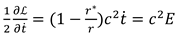
NB because of the multiplier used, is really an equivalent contra variant angular momentum rather than a covariant one, so that this setting seems like to insert the contra variant conservation in. It is said that the setting of does not coincide with general covariance. Even so, we will find out that it is exactly wrong setting so that the setting of constant should be required to give not bad results.
Then the Lagrangian would be treated to be
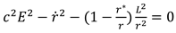
Setting , , and then , there is
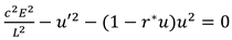
Derivated by , it is
At a farthest position the right hand item goes to zero, then the equation will have a solution , where is a distance from solar center to the asymptotic line. Replacing the very small right hand item with the solution, there is
There is a particular solution
Then the approximate solution of Eq. (337) is obtained

For an infinite large , the is infinitesimal one, there is

Observational deflection case is
 where is the radius of the Sun.
At the position and , there is
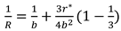
or

That will bring about contradictions for the setting of Eq. (333) that at peak point there is
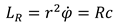
while at a very far point, there is
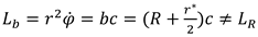
It is said that the equations have been solved incorrectly. Might as well, we could find out an inevitable solution after the inappropriate setting of Eq. (333) in next section.
8.4. Revisit Equations of Light Ray Deflection
8.4.1. Errors Hidden in Classical Equations
It is obvious that a wrong setting has been made in Eq. (335), because in gravitational field, really varies with . In fact, the Eq. (332) could be solved directly as following.
Considering , the Lagrangian really is

or
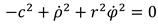
It is really the composition of light speed in covariant space.
Transform the equation as
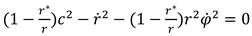
If setting peak point radius as and the angular moment at that point , with , it becomes

To be derivated by , it is
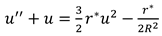
With instead of , it becomes
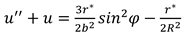
Because, it could be solved as
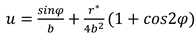
One will obtain the solution of the equation as

At the peak point as , we will get the constant that
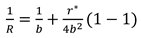
so that

Mathematically, this equality indicates that the solved line is not a natural line, in that if the curved line and its asymptotic line have same coordinates at start point and end point, there must be an inflection point on the curved line.
And the setting of Eq. (333) has been well kept that
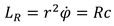
and
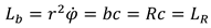
This is really the inevitable solution for classical equations but it is not a true result for realities. We have seen that the classical equations to have been solved to an answer Eq. (340) accurately up to the observation results is just caused by the wrong settings of energy momentum conservations of Eq. (333) and Eq. (334). It is said the classical equations do involve with problems while the wrong settings do.
8.4.2. Momentum, Energy and Angular Momentum Conservation
We have drawn the conclusion that light momentum keeps conservation in contra variant space rather than covariant space, and then of course, so does the light mass energy. In fact, apparent light speed or so called contra variant light speed may varies in contra variant space, but light momentum and energy will not be affected by apparent speeds. In fact, neither geodesic equation nor the derivations of Lagrangian could help proving the Eq.(333) and Eq.(334), in that Eq.(333) and Eq.(334) are substantially not correct.
Considering a light ray goes a vertical distance on the Earth, one could gain the mass variation as
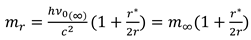
It could be called simplified equation of mass in gravitational field.
Light momentum could be expressed as
or the momentum square

Case in contra variant space, apparent light speed varies with position so that that speed cannot be used in expressions of light momentum directly. The invariant light speed could be seen as absolute light speed. Eq. (360) performs full variation with gravity by , which is the performance of momentum conservation. In fact, light momentum depends on frequency, just as does. If we ask more for a deep reason, that should be mass energy equation.
Case in covariant space, if light momentum will also be expressed by frequency, that will vary with bases additionally.
We know the Lagrangian
With Lagrangian substituted in conservative momentum square, it turns to be
or
As we have discussed, light speed cannot be directly composed in contra variant space but can be done in covariant space. This is a reason the Lagrangian is employed in conservative momentum square.
In one source fields, the momentum vector could be discomposed to be components of centripetal and tangent

or
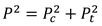
Obviously, the tangent momentum relates to tangent velocity and centripetal momentum relates to centripetal velocity. It could also be inferred that the tangent component varies with the corresponding velocity, and so does the centripetal one.
So that there must be
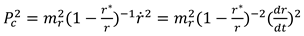
and
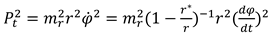
In one source field, the angular moment conservation could be expressed as

It should be highlighted that we are talking about the moment conservation in contra variant space. It is amazing that the angular momentum should be expressed in the form of rather than the form of , or we have seen that light momentum could be only directly composed in covariant form. The real reason is that the invariant light speed is just employed for the expressions by invariance.
The issues of light momentum have always been one of the controversies in physics for more than a hundred years [18]. The main problem is the difficulty of assessing the light momentum in transparent materials between Minkowski’s equation [19] and Abraham’s equation [20]. To one’s surprise, we would have made the conclusion different from both of them, after the discussions in previous sections, because of Lorentz covariance.
Nevertheless, angular momentum brings about new surprises on it. We will find that the surprises not only rise up from the expressions, but also hide behind the kinematics of light propagations in gravitational fields. These efforts might bring about tiny contributions for the attempt to answer the question of Einstein about 'What are light quanta?'[21] I appreciate what Leonhardt has said that light continues to surprise [22].
8.4.3. Revisit Equations for Light Ray Trajectory
We have recognized that it is conservation principle that really controls the solutions. In fact, light rays in gravitational field may experience mass energy variation.
As has mentioned previous, the light mass at the peak point is
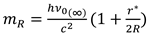
And it varies at position
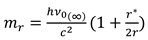
These two equations involve the energy conservation in contra variant space rather than that in covariant space.
For a light ray passing by a one source field, there is the angular momentum conservation as
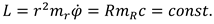
It should be highlighted again that the contra variant light momentum has been expressed by and which are of covariant space quantities rather than and of contra variant ones. In fact, it could be proved that and cannot be taken to form momentum conservation, if one takes efforts to have a try. That is because momentum variation is depend on that perform the effect of gravity, or in another words, the gravity input energy into the . The invariant light speed employed reveals that light momentum variation really depends on frequency rather than real velocity, just as that light propagates in transparent materials. That perhaps is really surprise.
Considering the Eq. (370) and Eq. (371), there is
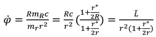
where . In weak field, the item , thus

I prefer to present the Lagrangian again
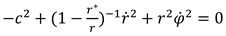
Define , so that . There is
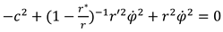
Insert the Eq. (374) into it, so that

With , it is
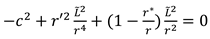
With , and it turns to be
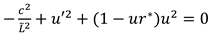
We have seen the similar form of Eq. (336), but this equation comes from the settings of the real conservation principles.
Differentiation results in
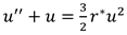
Case is very big value, the equation could be simplified as

It could be solved to be

It is a horizontal line with a perpendicular distance to the center of the Sun.
The right item of Eq. (380) could be replaced with the simple solution, because the deviation is also very small. So that the equation could be reformed to be
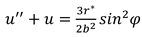
Once again, we could obtain the solution
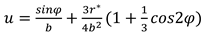
And then the deflection angle

Case , there is

Because it becomes

or

To verify the momentum conservation that

At a position
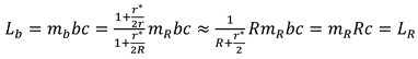
It seems that we have got the same results as that of classical equations. But the truth is that the solution is the results after the conclusions of momentum and mass conservations which completely others to that of classical theory and at the same time the assumptions of Eq. (333) and Eq. (334) are thoroughly given up.
The most important is that the real kinematics of light propagation has been discovered.
8.5. More Discussions
The trajectories of light ray in gravitational fields have more details behind the previous solution. Further analyses may help to discover more realities.
8.5.1. Detailed Discussions on the Coordinates of the Light Ray Trajectory
Further discussions are going to be sponsored to make more detailed analysis for understanding of some items, positions and their calculations.
Item 1 is to recognize various kinds of lines. The most important line is the real light ray that is emitted from a farthest star to the observers on the Earth. This line should be curved as it goes closely to the sun. Prolonging the straight parts of the light ray, one will gain the crossed straight lines, the asymptotic lines of light trajectory. They will be parallel to the two radial coordinate vectors left and right. There is another important line is the straight line from farthest star to the observer, that will present the real star direction from observer to the star.
Item 2 is to recognize those angles. is the second coordinate of farthest point on the light ray. Because the Earth is far enough to the Sun, the elevation angle of observer view line could be seen as . And because the star is very very far from the sun, the angle between straight line to the star and horizontal line could be also seen as . Thus the total deflect angle of is approximate . They could be shown in Figure 19.
For the coordinate of the Earth, , where is astronomical unit, the simple solution could be used

where, is second coordinate of the Earth.
Thus, there is

Because we know that , where is solar radius, so that
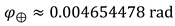
The height of the horizon line to light ray
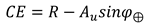
It is difficult to get a not bad accurate solution. However, we can turn to discuss the value of instead. For the approximate of , it could be gain
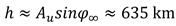
in the upper height , there is a very small difference between real ray trajectory and asymptotic line, the .
For the condition that light rays run from farthest position to the position they pass by the Sun, there is the equation after angular momentum conservation
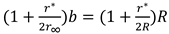
NB, is perpendicular length to asymptotic line, which is the moment distance for farthest positions, and only in approximate cases, it could be seen as . is peak point radius, and it need not be determined to be in these discussions theoretically.
Then it is easy to obtain

Peak difference between and is
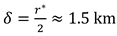
It is more difficult to investigate such a fine distance in practice that not only because of the observational accuracy but also due to the coordinating of the peak point of light ray. The development of very-long-baseline interferometry have the capability of measuring angular separations and changes in angles as small as 10-4 seconds of arc [23]. That shows probabilities for the quite good accuracy for fine angle measuring. This issue perhaps cannot be solved easily.
We can study the right branch of asymptotic line with an overplayed as shown in Figure 20.
There is the asymptotic line equation as
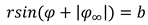
or
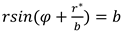
Case , we will see that the top point is close to the peak point
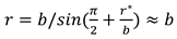
Case is not very close to , considering is very small, the approximate form of sine function is
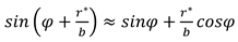
Thus, the deformed equation of asymptotic line could be written as
It should be pointed out that the equation or is a horizontal line with a perpendicular distance to the Sun center.
For the case that a light passes closely by the edge of the sun, there might be some influences from solar corona. It is a good idea to left a distance from the edge, for example, the position of or even further. But this idea is only for theoretical discussions. Hitherto, we could only observe light deflections in the conditions that light rays pass by the sun edge just fine, because otherwise, peak point could not be coordinated at all.
8.5.2. The Invalidity of Newtonian Second Law in Light Propagation
It is the most interesting that perhaps there is the probability to carry out new numerical method to calculate the light trajectory in gravitational field, which could be called ballistic trajectory method. Considering that the gravity component parallel to the motion trajectory will not bring about changes to further motion, we could only consider the calculation on motion variation due to vertical component of gravity so that to determine a differential coordinate on the trajectory. Thus, in the way incremental, the trajectory could be solved at last.
Firstly, it is proficient to take the motion of close-to-light-speed massive particle into discussions, as shown in Figure 21.
It is believed that for a massive particle in weak field, the vertical deviation could be solved by Newtonian second law

The coordinates at position are known to be or . As well, the trajectory will have a direction with angle . Then, the distance in a time interval the particle travelling is

The deviation angle of to is

and

Thus, the coordinates at position could be calculated as
or
It should be pointed out that the angle is not the direction angle . The could be calculated by angular momentum conservation.
where, .
Now back to the fly of light ray from position A to position B. It might be imagined to calculate the deviation also by Newtonian second law. That sounds naturally to see the photons as light speed particles with dynamic mass so that to deviate in the same way as massive particles do. Unfortunately, it is impossible in that that kind of calculation will lead to the result very close to that of massive particles. It seems like that the Newtonian second law sounds invalid in light propagation even at the vertical direction.
But there is still an opportunity to explore the ballistic trajectory method for it. That is to perform by trial method. We can imagine that after point A there will be a wave front after Huygens’ postulation, then, some points on it may be selected for further considerations. With angular momentum conservation and Lagrangian, one can calculate the velocity and angle as shown in Figure 22. Thus, the deviations of the points could be estimated to help for further trial. I have made more efforts to try but not done, although I still believe the probabilities.
8.5.3. A Wrong Treatment for Light Propagations
If the covariant angular momentum conversation would be insisted for light propagations as
It is seemingly that presents the contra variant angular velocity of photons which is expected to correspond to contra variant angular momentum. And moreover, it could be argued to take as expressions of contra variant angular momentum, that will exactly lead to conservation break as gravitational redshift is concerned.
Now for the equation Eq. (413), there is
where . In weak field, the item , and , thus

Because the Lagrangian with coordinate time is
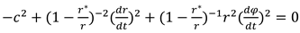
It could be transformed to be
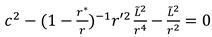
or
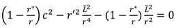
Consider again

To be derivated to be
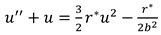
It could be solved as
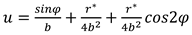
One will gain obtain that

One can verify the peak point on the case of , and , and then will gain

That has broken that principle of angular momentum conservation. Of course, it is a wrong answer for light ray propagations, because of a wrong setting.
8.5.4. Equations of Close-to-Light-Speed Massive Particles
We have known that massive particles will not run with general covariance. They run with Newtonian laws. The velocity composition for close-to-light-speed massive particles really is
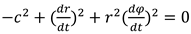
The conservation of angular momentum
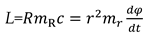
One will find that is used here is because the velocity composition equation Eq. (424), which is rare different from the Lagrangian for light. The constant is not the speed of light while it really is the approximate speed of massive matter. So that the in Eq. (424) is just a velocity composition of close-to-light-speed motion. The Eq. (424) and Eq. (425) perform the differences of conservation between light fly and the motion of massive matter. We will see these differences in the equations of low velocity motions of massive matters in next sections.
The angular velocity
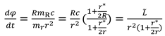
where . In weak field, the item , and , thus
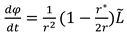
Together with , the Eq. (424) turns to be
or
With , and , and considering , there is
To be differentiated as

It could be solved as
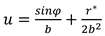
Obviously, there is

It is easy to calculate in Eq. (432) that at the peak point, , and , so that

Or with angular momentum conservation there is

Again, we obtain

The asymptotic line
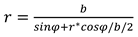
It is said that the trajectories of light rays and close-to-light-speed particles present different but the same peak difference . The same peak difference is just the result of momentum conservation.
In fact, these studies have help to create the dynamics of close-to-light-speed particles in gravitational field. By the way, one can compare this solution with that in section 8.4.1 that they have both given the same result of , but they gave different value of .
8.5.5. Comparisons of Numerical Solutions and Algebraic Solutions
To make comparisons with numerical and algebraic solutions is not only a kind of further verification but also a further support to the conclusion of energy moment conservation. As has discussed previous, ballistic trajectory method could be developed to calculate the trajectories of close-to-light massive particles. It could be applied by dividing trajectory to finite segments and calculating coordinates with Eq. (404) to Eq. (412) step by step. The invalidity of Newtonian second law for light propagation is actually another kind of support to the inferences of kinematics.
Notwithstanding, difference method for all differential equations could also be employed for more comparisons. Difference method has shown great advantages in scientific calculations and many excellent schemes have been developed to serve for more complex requirements.
For the equation of light rays
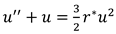
The simple central difference scheme could be suggested that
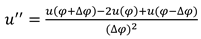
Thus, the difference equation could be built as
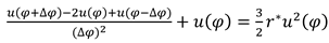
Pre-exercises show that if step intervals defined by , the calculations would get quite good accuracy.
As for the equation of close-to-light massive particles, the differential equation

The difference equation could also be built simply as
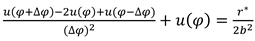
Thus, we would sponsor a comparison with the analytical solutions, difference method solutions and the ballistic trajectory method solutions mentioned previously, together with the asymptotic lines and horizontal line for references.
Numerical methods of difference and ballistic were carried in office computer and others were completed by the calculator of my mobile phone, in that the phone calculator could provide 8 floating point precisions more than that of the Fortran software in the computer.
It is shown in Table 3 that difference method and ballistic method still perform not bad precisions in the results of upper parts of the trajectories. Of course, both of the two methods are of step by step arithmetic so as to accumulate quite amount of deviations at the rear parts of the trajectories, especially for that of ballistic method. Anyway, the two numerical methods are reliable, that greatly supports the inferences of kinematics.
It easy to develop more optimal schemes for difference method and the way of optimal secant seeking instead of the tangent seeking for ballistic method or any other effective technologies to improve the precisions of numerical analyses. That will confirm the conclusions and inferences that have been drawn previous.

Table 3.
Comparison of the analytical solutions, difference method solutions and the ballistic trajectory method solutions.
Table 3.
Comparison of the analytical solutions, difference method solutions and the ballistic trajectory method solutions.
| coordinate angle | coordinate radius (m) of solution of light ray by method of | coordinate radius (m) of solution of close-to-light-speed massive particle by method ofmassive particle solution of coordinate radius | coordinate radius (m) of | |||||
| (degree) | analytical | difference | asymptotic line | analytical | difference | ballistic | asymptotic line | horizontal line |
| 90 | 695500000 | 695500000 | 695501477 | 695500000 | 695500000 | 695500000 | 695501477 | 695501477 |
| 80 | 706229140 | 706229166 | 706230180 | 706229186 | 706229216 | 706229226 | 706230444 | 706230708 |
| 70 | 740135345 | 740135367 | 740136069 | 740135540 | 740135570 | 740135590 | 740136641 | 740137212 |
| 60 | 803093469 | 803093487 | 803093961 | 803093961 | 803093991 | 803094020 | 803094945 | 803095929 |
| 50 | 907909142 | 907909153 | 907909463 | 907910181 | 907910213 | 907910251 | 907911080 | 907912699 |
| 40 | 1082002548 | 1082002549 | 1082002744 | 1082004645 | 1082004679 | 1082004738 | 1082005482 | 1082008219 |
| 30 | 1390992617 | 1390992592 | 1390992723 | 1390997047 | 1390997085 | 1390997170 | 1390997839 | 1391002954 |
| 20 | 2033486508 | 2033486403 | 2033486554 | 2033497655 | 2033497694 | 2033497838 | 2033498416 | 2033510279 |
| 10 | 4005136911 | 4005136314 | 4005136922 | 4005184405 | 4005184395 | 4005184750 | 4005185149 | 4005233377 |
| 0.26 | 153123772603 | 153122660623 | 153123772604 | 153195382906 | 153195143112 | 153195397701 | 153195383644 | 153267061697 |
| 0.01 | 3890278441952 | 3889557122200 | 3890278441977 | 3937035389754 | 3936873242381 | 3937033549851 | 3937035390479 | 3984929947953 |
| 0 | 163784893532900 | 162515766173612 | 163784893516163 | 327569787065801 | 326450054739264 | 327616498942582 | 327569787031587 | ∞ |
8.6. Time Delay of Radar Echoes
For a light ray passing by the Sun, the velocity varies with the positions and directions on the trajectory. There should be a difference between the real time interval and that calculated via invariant light speed instead of apparent light speed. Shapiro proposed new tests of time delay of radar signals which transmitted from the Earth to pass by the edge of the Sun to another planet or satellite and then reflected back to the Earth [24,25]. The observations on time delay of radar echoes would forcefully support the theory of general relativity as well as that of light ray deflect.
However, the solutions of time delay must have involved in the problems with light trajectory, that the solution process has inherited the errors in classical equations of light trajectory, so that it is necessary to make a detailed discussion to rectify.
8.6.1. Classical Solution
In classical procedure, with the assumptions of and , the Lagrangian could be transformed to be
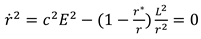
And also with
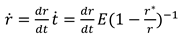
The Lagrangian becomes
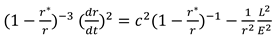
At the peak point, so that there is
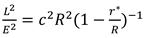
Where, is the coordinate of the peak point.
Taking it back into the Eq. (445), there is

or
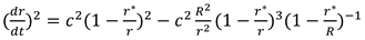
The differential relationship could be integrated that

Because and are very small, it could be written as
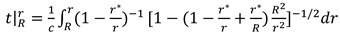
It has an approximate form [4] as
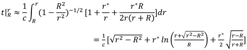
8.6.2. Errors in
We have known that the assumption in classical equations is incorrect. In fact, the equation could be solved without the assumption. Such as the Lagrangian
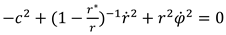
With it is
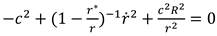
And we know that
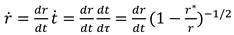
so that
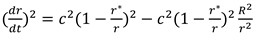
The differential relationship could be integrated that
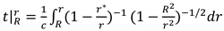
Approximate solution is
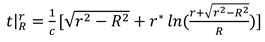
One can find that this treatment has just brought about a little deviation from the previous. That is because the trajectory is only a little different from that one at deflect angle.
8.6.3. Revisit Solution for Radar Echoes
The revisit equation of trajectory may help to get new performances of the issue.
For the Lagrangian
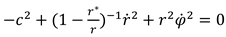
In previous section, we have got the angular velocity expression based on energy momentum conservation as discussed in previous sections that and , where
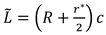
In weak field, the item , thus
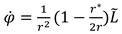
Then the Lagrangian becomes
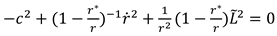
A transformation could be made as
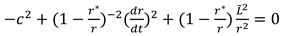
With Eq. (459) it becomes
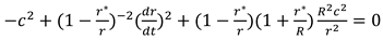
so that there is
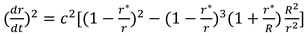
or

or
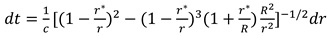
Integrate above differential to be
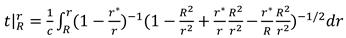
or
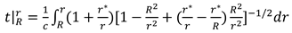
By building a function

where, . The derivative
Considering is very small, the rear part of the integral could be simplified as

Then the integration could be gain as

where in the last item, a has been simplified to be 1.
The first part of the integration could be calculated to be

and the last part is done as

so that the total integration is
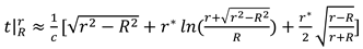
8.6.4. Solution for Close-to-Light-Speed Particles
Now let’s discuss another kind of no delay time spend, the time spend of close-to-light-speed particles. The velocity composition of close-to-light-speed particles could be expressed as
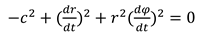
With angular momentum conservation, there is
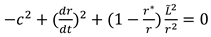
or
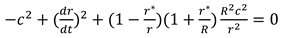
so that the integration could be built
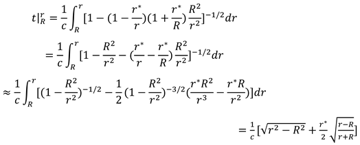
We have found that the revisit solution of time spend is the same with classical. The reality is that the classical treatment has got the same trajectory by additional settings, so that it is undoubtful to gain a same time spend with.
8.6.5. Equations of Time Delay
In fact, the problem of time delay of radar echoes is just a kind of performance of light deflection. The results in these discussions are also just extensions of that in the problem of light deflection. The classical equation for time delay is to defined the difference between time interval of light rays and motions of absolute light speed, and the length of the trajectory has been coarsely set to be
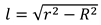
So that the classical equation of half branch time delay could be calculated as
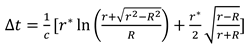
But the half branch time delay of light rays, with respect to the time interval of close-to-light-speed particles Eq. (479), will be a little different
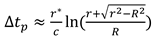
One may argue that the trajectory of close-to-light-speed particles will be different to light rays. In fact the real length of the light trajectory also does not equal to . One can easily take measures to work out the real length of that trajectory. I prefer to give a more accurate value than Eq. (480) that could be estimated by geometrical relationship while that

where, is deflect angle of light ray.
So that a real half branch time delay of light rays with respect to an absolute motion on the very trajectory is

We know that the time delay has been verified to be very high accurate value with respect to the classical equation, that is because the trajectory length has always been set to be , which is indeed not accurate length of trajectory line.
If consider the close-to-light-speed particles, the real length of its trajectory line could be estimated to be
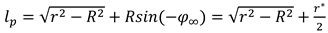
where, is deflect angle of particles.
With Eq. (479), the half branch time delay of close-to-light-speed particles is

This result of close-to-light-speed particles is really a spectacular inevitability of kinematics rather than occasionality.
Something different from trajectory investigation, the test of time delay of light and close-to-light-speed particle propagation might allow a quite big separation to the Sun edge thereby to provide not bad accuracy. Furthermore, it could be expected to sponsor an experiment to emit light rays and massive particles on a straight line from a point not very close to the Sun at the same time for time delay comparisons.
8.7. Equations for Un-Close-to-Light-Speed Massive Particles
Let us investigate a un-close-to-light-speed motion for massive particles from specific position to another position . Considering a variable mass , the gravity
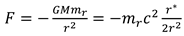
Dynamic energy converted from gravitational potential by a motion from to is
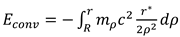
and the total energy
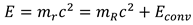
The function of total energy could be written as
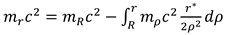
Setting energy at position as a known quantity, it could be differentiated that
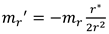
It could be integrated to be
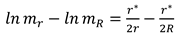
Then we gain the expression of variable mass that
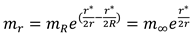
where is the mass at a farthest position. This equation could be called general mass equation in gravitational field.
And we would like to carry out the expanded expression of gravity equation that
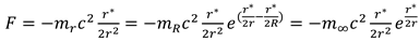
One could find that the relativistic mass may not keep mass conservation any more that may surprise us, but it really has been revealed in realities. This is another kind of comprehensive physics which I will not make further discussions in this section. Mass of matter does matter [26]. The truths stay in realities.
Dynamic energy will be converted as
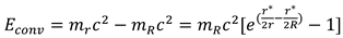
It should be pointed out that the expression of exponential equations of mass variation of course could be used for light ray propagations and close-to-light-speed massive particles for higher accuracies case in strong fields.
For massive matters, with special relativity, the equation of dynamic energy at a position is
 where, , see Eq. (304).
In gravitational field the dynamic energy varies with position that

Conversion energy could be positive case potential release or negative case potential withdrawn. However, dynamic energy always great than zero, so that the variable will be limited in some specific cases that depends on initial conditions.
NB, for the convenience of expressions, the tensors of velocities, frequencies or the components maybe not written in tensor format anymore case they may not bring about confusions for understandings, for examples, and refer to the velocity at position and .
It should be further discussed here that we have seen dynamic mass energy may come from the release of gravitational potential. That will then perform as inertial mass and gravitational mass. If in two source system, they move closer or farther will cause mass increase or lose in that we incline to realize that potential does not act as mass. We are not sure that in this condition mass conservation is available or not. I am inclining to say no. In this section, this controversy does not really matter. This discussion just presents the issue for more focus.
We now prefer to study the conditions of irrelativistic velocities so that , and after Eq. (493) and Eq. (497), there is the velocity square
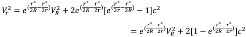
As we have discussed, Lagrangian could no longer be employed for analysis on the motion of massive particles. In some publications, the so called Lagrangian for massive particles is classically defined to be as [3,10]
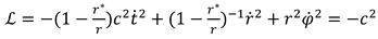
In fact, it could be easily deformed to be
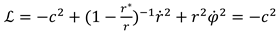
That will lead to obvious errors that
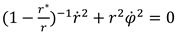
That means a zero velocity composition. It is impossible to interpret realities with. We know that in classical equations, the assumption of has still been employed to solve the problem. One might be involved with more errors to solve one more error.
After conclusions and inferences previous, for a massive particle in one source gravitational field, the velocity composition could be expressed as
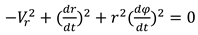
This equation could also be performed for that of close-to-light-speed massive particles as , as Eq. (424) and Eq. (476), where these discussions have not been released because of consideration of reducing arguments.
With angular momentum conservation, there is
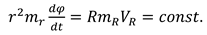
Of course, the angular momentum conservation for lower velocity motion will be the same as that of close-to-light-speed massive particles. But they are really different from that of light rays.
So that
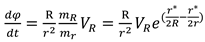
In which and are velocity and mass at peak point, where .
Together with the Eq. (498) and , the Eq. (502) becomes

or

Setting , it is

To be derivated by , it becomes

To take the one-order approximation for those exponent functions, the equation becomes

One can also get this equation in simplified ways, but that will also experience comprehensive complexities while the way above seems more physically explicit. The exponent function forms used here is also to present more primary expressions of mass energy. In the conditions of strong fields, the exponent forms may take effects. One can see that the kinematics of light or close-to-light particles could also be expressed in more primary ways.
In weak fields, those very small items in Eq. (509) will be neglected. That becomes
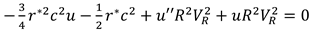
or
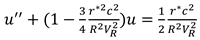
Setting
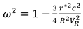
For planets in solar system, the last item in Eq. (512) is far less than 1.0, so that
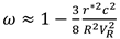
For planet trajectory, the equation could be solved as [27]
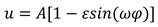
With this solution substituted back into Eq. (511)
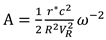
One-order approximation of Eq. (507) is

Neglecting very small items, it is
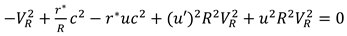
With Eq. (514), it becomes

Case there is

So that the eccentricity is
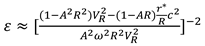
Some publications have given the following expression for eccentricity
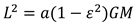
where, has been set the angular momentum.
But this is not a real solution for eccentricity, because that the Eq. (514) shows .
We will then prefer to present the perihelion precession of
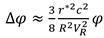
or the precession per revolution
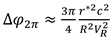
The most surprising is that this solution of perihelion precession is really irrelativistic. It is a half of the value of the classical solution. It is practicable to carry out more experiments of motions closely around the Sun to verified the conclusions of Eq. (522).
One can focus on more sophisticated conditions for massive matters traveling in gravitational fields, based on the Eq. (508) or the Eq. (511), especially for those motions in strong fields and with high velocities.
Perhaps this result is the only one in which we have focused on that is in contradictions with the observations that have declared perihelion precessions of planets in solar system [17]. But some observations on PSR J0737-3039A/B [28,29] have shown quite big deviations from classical predictions, which had been expected to have perihelion precession together with geodetic precession. Nevertheless, the experiment of Gravity Probe B [30] shows that geodetic item has got accurate results while frame-dragging item hasn’t, in which it could be recognized that the geodetic item is really the effect of special relativity. Observations on S2 [31] and PSR 1913+16 [32] also cannot provide positive supports for the predictions of perihelion precession of classical theory.
9. Relativistic Release and Relativistic Frequency Shift
It is predicted that in one source field, the inflow of matters may cause relativistic release. Sole matters moving to the source center for a separation is exactly a kind of inflow, of course. But I want to point out that the inflows of accretions of active galactic nuclei are really normal performances in celestial evolutions. As the matter of facts, they have not been well investigated, so that it is necessary to cast a few concentrations on.
9.1. Dynamics of Active Galactic Nuclei Accretions
9.1.1. Galactic Nuclei Accretions and Planet Rings
The discovery of active galactic nuclei is one of the greatest advances in the proceedings of the astronomy in the 1960s [33,34]. Active galactic nuclei are of the most spectacular extragalactic objects not only because of their extraordinary giant radiations [35] but also due to the complicated spectrum and high red shifts. The emission spectrums of active galactic nuclei are really non-thermal continuum [36]. Those issued models for active galactic nuclei in the past decades, such as the so called standard model [37] or unified model [38], have not really interpreted the mechanism of accretion inflow and energy release. This is the reason that I want to sponsor a brief discussion on the dynamics of active galactic nuclei accretions.
Active galactic nuclei accretion disks exactly experience resemblant kinematics with planet ring systems in that both of them are of surrounding dusts revolving the center source, loosely inside the Roche limit [39]. I am going to sponsor a study firstly with respect to the planet ring systems so that to renovate those recognitions upon the evolution and fueling mechanism relating to active galactic nuclei accretions.
Planet rings are not static structures [40,41]. Their evolutions involve with numerous internal and external processes in which Keplerian shear acts the key role. It causes rings to spread [42] in all process. As we have seen, Saturn rings usually have that striking refined structures.
In the condition that ring particles are small enough, the electromagnet interactions will then overcome the inertials so that to control the motion within the rings. Such particles or together with gases getting to form colloid, will as a whole to perform fluid behaviors so as to bear pressure. Under the driving effects from outer boundaries, a fluid ring may go cubically bolder because pressure increasing helps particles to move deviate vertically to the ring plane, such as the Halo ring of Jupiter [43]. Spectrum observations predict that the particles in Halo ring are less than submicron. Optical observations also show that Halo ring seems blue and gray with respect to that the main rings show red color [43]. It is because that the fine particles scatter more blue rays, just like our sky does, while coarse particles scatter more red.
Firstly, I want to make a discussion based on a fluid ring in the condition that the center velocity equals to Keplerian velocity.
9.1.2. The Structure of Fluid Rings
For Keplerian motion of matters around center object, there is
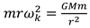
where, is mass of a particle, is gravitational constant, is the mass of center source, is distance to the center and is angular velocity while is tangent velocity.
The tangent velocity and angular velocity will increase as radius getting smaller that
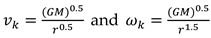
Keplerian kinetic energy could be expressed as
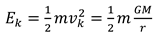
Keplerian motion means constant angular momentum for a particle at specific position.
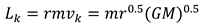
Namely, there is Keplerian shear at the specific position, and the shearing rate can be derived to be
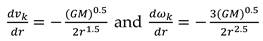
We will start from a simple condition that a fluid ring has a Keplerian velocity at its center position. For a differential element at a position of radius in the ring, there could be unbalanced force between gravity and inertial force on the plane of rings. The reasons of unbalanced force may come from low velocity matters falling from outer rings, the driving force, or the resistance of inner parts which have higher velocities and be restrained by outer parts. These interactions in a ring may lead to bold ring as Figure 23 shows, that really others to the flat rings as that of Saturn.
This unbalanced force will be rebalanced by pressure gradient, which will take the part to form the fluid pressure. For example, in the outer part of a fluid ring, if the velocity is lower to form driving force, the pressure could be calculated as
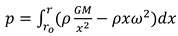
where, is density of fluid, is radius respective to the outer edge of fluid ring, and the angular velocity is less than Keplerian angular velocity of the very point and greater than the center one so that to give driving force. If a linear function is defined as
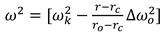 where, refers to radius of pressure center and represents the angular velocity square difference with respect to for the position of outer edge point. It interprets active falling down of the outer part because of losing of velocity.
Concern that at every position there is the relationship

The Eq. (529) becomes
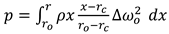
We know that the pressure of inner edge and outer edge equal to zero. Concern There is an approximate solution of center pressure
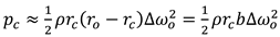
where, represents outer radius of fluid ring.
On another side, the resistant force determined by the higher velocity of inner parts, with velocity as
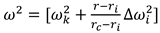
In which is greater than so that to form a passive resistant force.
There will be the center pressure
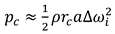
where, represents inner radius of fluid ring.
On the direction vertical to the plane, it is easily to calculate that
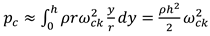
where, represents vertical height from top or the bottom to the center of the ring, is the distance to pressure center and is Keplerian angular velocity at pressure center.
Thus, the relationships between semi axes are


The outer side of the ring may be called driving side, depending on a random falling of outer particles, that forms an ambiguous boundary. The inner side of the ring comes from passive driving, may be called driven side, so that to form a sharp edge as seen in Halo ring [43], just like water surface in an accelerated container. Of course, fluid rings also can be flattened and split to be refined structures so that performs more complicated than Halo ring.
I just want to point out that there is a special condition that
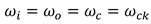
Thus, the whole ring will have a unified velocity so that there will be no Keplerian shear in the ring. And then
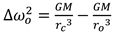
as well as
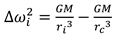
and

That will lead to an equilibrium state that the ring stops evolving because of Keplerian shear vanishing. But this state may need strict conditions and may be destroyed by outer influences in a long term. Halo ring might have reached an approximately equilibrium state which could be investigated by detailed observations in the future.
Secondly, I want to discuss the split of a ring under the condition of developed Keplerian shear. If a fluid ring is well Keplerian sheared, it could be predicted that the ring will go thinner. We know that there are Keplerian shear at every position in the ring. But we can make an analysis on the angular momentum conversion in the middle point which could then at last split the ring to two parts. For convenience, it could be defined as two rings originally, the ring and the ring as shown in Figure 24. They will have their own Keplerian velocity points at and . In a time interval, the two rings will complete quite amount of angular momentum conversion because of the Keplerian shear, which is just like viscous friction acts in the interface that makes the conversion.
Setting the mass of rings , the relative angular momentum difference between two neighboring rings could be estimated as
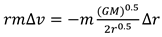
where and
The exchange of angular momentum may be expressed as
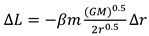
where, momentum exchange ratio .
It is said that after a Keplerian shear, the outer one should get increase of angular momentum and the inner one should get that decline. For the reasons of kinetic mechanism, both the inner ring and outer ring will be driven apart from original position. If inner ring goes a difference , the difference of Keplerian angular momentum could be calculated as
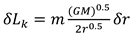
Let equals to , it is obtained that

For the inner ring, it goes to shrink by falling a (minus) separation so that to form a new state. And for the outer ring, it expands by going up to a (positive) separation.
We have seen that this is not a whole dynamic analysis because that the pressure in the ring has also taken the effect of angular momentum conversion, but that does no harm for the conclusion that Keplerian shear, i.e. the viscous shear in the ring, leads to angular momentum conversion and rings split. One can make detailed study with Navier Stokes equations.
It is said that a process of rings spreading around a source center is an irreversible process with entropy production.
9.1.3. Shearing Dissipation in Fluid Rings
This issue is carried out to estimate the shearing dissipation so that to discuss the evolution by Keplerian shear. Of course, the evolution would involve together with momentum conversion and rings split. But in the aspect of theoretical methodology, it is better to be investigated in two steps, the angular momentum conversion by Keplerian shear, and the energy momentum conservation during rings split.
Angular momentum conversion must be done across the interface between the two rings, so that the first step analysis is reasonable. I prefer to focus on the states before and after momentum conversion of two neighboring rings. Before conversion, the neighboring rings have been separated by , with velocities
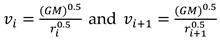
The difference between and is
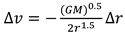 where is defined as minus quantity while as plus. Namely,
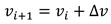
Considering ring mass equals to each other, two conditions would be taken into study.
As angular momentum conversion happens, there are

As has been defined minus, the inner ring is really slowed down and the outer ring is accelerated. Because of , kinetic energy may not keep conservation. With original kinetic energy of
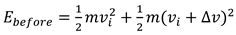
and the kinetic energy after conversion of

Thus, there is the dissipation energy without considering potential variations

Considering the Eq. (549), it turns to be
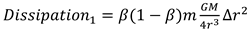
Then we will go to the second step. After the first step of angular momentum conversion, the outer part of inner ring loses momentum so that provides driving force to drive the inner ring to inflow and the inner part of outer ring will be accelerated to higher momentum so that to compress the outer ring to outflow. This evolution will perform a little sophisticated in that the inflow ring should be accelerated by gravity and the outflow ring should be slow down by gravity. We know that the inflow of a ring will cause half potential release surplus with respect to the Keplerian energy requirement and the outflow will experience potential withdraw. And also, we know that the gravity is perpendicular to the rings. These issues could be solved in fluid flow anyway, for example the evolution of vortexes. But we are just going to check the energy conservation of final state.
After the inner ring inflows a separation and the outer ring outflows a sepration , they come to a new state of Keplerian balance. Taking the inner ring for granted, before Keplerian shear, its total energy involves with Keplerian kinetic energy and potential
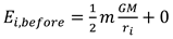
After Keplerian shear and inflowing a separation , total energy becomes
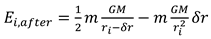
and for outer ring, the energy before
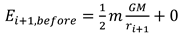
The energy of final state
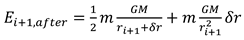
Energy difference could be estimated by
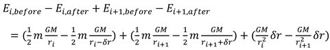
The first two items could be transformed as
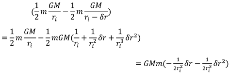
The middle two items could be transformed as
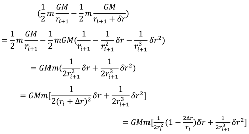
so that the previous four items are
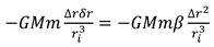
The last two items are
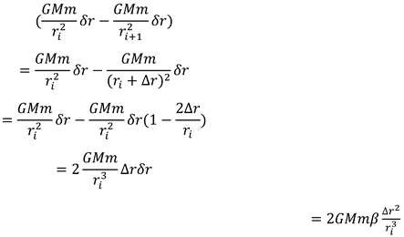
The energy difference is total energy dissipation
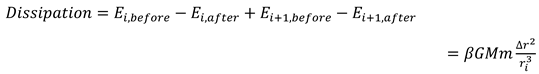
One can calculate the gravity potential release of a single ring inflow, although it does not sound reasonable for a comparison with dissipations because there is another ring outflow. Anyway, that is
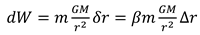
Thus, we get the ratio of dissipation and potential release
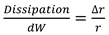
Or the ratio of dissipation-1 and potential release
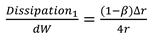
where .
Rings evolution dynamics indicates that the inner half of an accretion inclines to inflow and outer half outflows by and large. Additionally, the process of vortex evolution would dissipate, even though the two dissipations are not independent.

It shows that the dissipation in vortex evolution might be greater than that in momentum exchange between rings.
We know that inter-rings separation would be far less than the radius of relative rings. It is said that in the condition of Keplerian shear, the dissipative energy is a higher rank infinitesimal quantity of that of potential release of inflow, no matter that inner ring potential release will support the outer ring potential withdraw. Classical quasars could have luminosities of 1045 erg s-1 to 1046 erg s-1 [44]. It is unimaginable that those releases completely come from gravitational potential energy.
9.1.4. On Particle Rings
For solid particle rings, it is difficult to make a simple analysis on angular momentum conversions and on ring’s evolutions. In fact, any collisions between two particles might cause great changes for their trajectories. It could be imagined that for numerous particles in neighboring rings, assuming very small velocity difference between every Keplerian collision particles, we can predict quasi fluid behavior for Keplerian shear acting on neighboring rings, that in a whole, Keplerian shear help to make angular momentum conversion and rings split. One can also write down those equations of energy momentum just as that of fluid rings. But all in all, particle rings cannot form pressure so that they will only spread as a very thin disk with perfect and refined structures in the equator plane, unlike the fluid rings, which will form a bold 3-dimensional torus structures. I believe that numerical method could be expected for quasi fluid behavior simulation for Keplerian shear of particle rings, as the effects of the rings of Saturn have shown us.
9.2. Relativistic Release
Any efforts to conceiving the mechanism of relativistic release would encounter great difficulties, because of two reasons that relativistic release has not been well recognized and we still know less about the intrinsic structures of fundamental particles that would be seriously related to relativistic emissions. But on the other hand, tremendous of observations have shown incredible probabilities for intrinsic emissions and correlated pseudo redshifts, as well as intrinsic redshift of absorptions, which are so intensely corresponding to the inference of relativistic release that I cannot help to make a try.
Despite the complexities of relativistic release for a massive matter inflow into the center source, I suggest a mathematic analysis based on an assumption of continuum release. It is still not a true expression of realities, but that may help for more understandings on that topic.
The apparent light speed could be employed to describe the concept of equivalent state in gravitational fields. It may be a state after relativistic release, although this state should be not really stable because there should be energy deficiency in the other two dimensions.
One can discuss the momentum exchange efficiency under the conditions of different apparent light speeds so that to talk about the variation of equivalent state. Another important clue that indicates equivalent state is the fine structure constant. We know that fine structure constant determines the dimensions of condensed matters, of course that may determine the dimensions of intrinsic structures. We can imagine that the variation of apparent light speed could bring about the variation of fine structure constant so that to bring about the variation of the energy of equivalent state.
I don’t think all of energy of a matter would take part in the relativistic release, for example, the most fundamental particles may be expected to be made of quasi photons, in common recognitions, they might not be split anymore. Thus, we would rather define the concept of releasable mass . I cannot give an estimation whether the maximum releasable mass should be up to or not, but it could be believed to be quite amount, where is total rest mass of original equivalent state, which corresponding to the state that the matters do not experience relativistic release.
Now for a center source field, equivalent state of matters is proposed to be

Matters located at different positions in the gravitational field perform different equivalent states. As a matter goes a separation along the radial direction, the expression of exceeding energy is
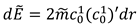
As a matter goes from the farthest point to the position of radius, the relativistic released energy could be integrated to be

Thereafter, we could also define a corresponding concept of the relativistic residual energy that, at a position, matters keep an amount of energy for subsequent releases,

It seems that the residual energy may go zero as matters reaches . It is just a solution of theoretical model. In practice, relativistic release will be intermittent, and matters perhaps to experience flattenizations as they close to so that to bring about instabilities. As results, residual energy may not go zero at the end in practice. This effort is just to manage to perform kind of probabilities of relativistic release.
It can be calculated that most part of energy is kept before
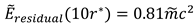
Now it is naturally to define the release rate by derivative of release energy along the radial direction to the center source. Released energy could be the integration of release distribution function from a position farthest to the position or the minus inversely
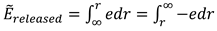
On the other hand, the residual energy could also be defined as an integration of release distribution from position to position or the minus form
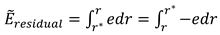
Thus, the release distribution could be derivated to be
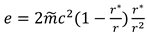
It is easy to calculate that the peak value locates at the position

with the maximum release distribution
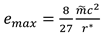
One can calculate the release intensity of accretion inflow. Setting equivalent mass for every single ring in an accretion, the luminosity could be derived as
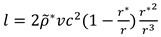
where, is matter’s assuming density at the position and is inflow velocity.
Suppose the accretion spreading sufficiently, it can be calculated that the most luminous area is at the position

As well as maximum luminosity
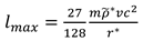
The Eq, (580) represents intensity of release at a specific position in an accretion disk. It is revealed that the peak luminosity should not happen at the edge of horizon event, but at a little outer position, just as that was shown in the event-horizon-scale images of M87 taken by the Event Horizon Telescope Collaboration with wavelength of 1.3mm [45].
9.3. Relativistic Emission Lines and Relativistic Redshift
Eyeing on the stimulated release of electrons in atoms, we could carry out a concept of exceeding ratio for relativistic release of an energy structure.
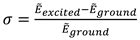
where and are energy of excited state and ground state of specific structure. Exceeding ratios for relativistic release may be more different from that of stimulated release of electrons, probably, they might be quite small or big. We know less about that.
In one source field, exceeding ratio would be variable with position as the so called equivalent state has shown.
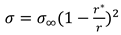
Thus, frequencies of specific emission rays could be written as
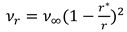
Case it could be simplified to be
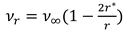
These emissions of course include but not limit to electron transition emissions that we are more familiar to that could be easily certificated comparing to stimulated release on the Earth. This kind of frequency will be quite different with which we have known well in weak field, in that it looks like redshifted after photons reach the Earth. But it is just a pseudo redshift because the emissions have not experienced real redshift at the emission time. The fact is that it is only verified to be redshifted by comparing to the spectrum characteristics of a matter in weak fields. In this case, it is just redshift seemingly. It could be called relativistic redshift.
In practice, emission lines will experience gravitational redshift to arrive a farthest position. The Eq. (493) could also be employed to interpret light mass energy variation in gravitational field, so that the detectable frequency could be expressed as
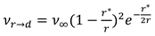
Case it could be simplified to be
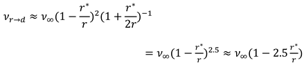
Propose a definition of relativistic frequency shift based on frequency
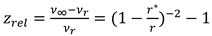
Case it could be simplified to be
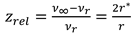
It is an intrinsic frequency shift rather than cosmological redshift. Note that keep invariant during propagation process if neglect the effect of gravitational redshift. is the comparative frequency of equivalent radiation in no gravity condition.
Detectable redshift should be calculated as
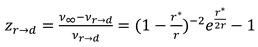
Case it could be simplified to be
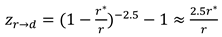
Relativistic frequency shift and detectable frequency shift could be calculated for comparison in Table 4.
9.4. Broad Lines and Narrow Lines
In the emissions of a quite amount of continuous inflows, the exciting width that the inflow involved sustains at radial direction may cause specific continuous emission distribution. As a result, that could be certificated to be a broadened line in spectrum diagram. For a massive accretion around a galactic nucleus, the Kepler shear may be employed to interpret the mechanism of inflow of a ring. If there is an inflow of a ring at position with exciting width of , the emission frequency may distribute from to . Considering the effect of gravitational redshift, one can get a line width expressed by frequency after Eq. (587) that

Case it could be simplified to be

or by wave length
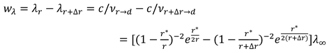
Case it could be simplified to be
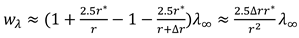
which could also be amount to a so called Doppler velocity by frequency as

or Doppler velocity by wave length as

where, is light speed.
Case it could be simplified to be

These equations show that in the region near to , relativistic emissions should have broader line widths.
Calculations on line widths of various conditions will be presented in Table 5.
It is said that line widths depend on inflow exciting width, but in totally analysis, they highly relate to the inflow positions. The regions close to may perform broader line than farther regions. Observations show that the sizes of broad line regions are estimated within 0.01 or 0.1pc and line widths are about 1000 kms-1 to 10000 kms-1, while the sizes of narrow line regions are about 0.1pc to 1kpc [48,49,50]. In fact, those certificated narrow lines incline to have been certificated as lower redshift lines. For radio emissions, some of them were observed to have compact cores and extended components [48]. The compact cores could be interpreted that equivalent state in inner areas of accretions would have lower equivalent energy to release lower frequency emissions, while giant extended components of emission pictures might be the jet outflow who emit radio lines.
Relativistic release must perform in sophisticated conditions. The most probable condition is that releases in one of the rings could overwhelming all of others, especially that of the most inner ring. Thus, in most cases, releases of an active galactic nucleus might be certificated by the emissions of the sole ring. One can find that most of narrow lines have been certificated lower redshift, such as NGC 4151 with z=0.0033 [51] and MCG-5-23-16 with z=0.00849 [52] have narrow Fe Kα lines. But on the other hand, their spectrums both involve with broad lines [53], that indicate controversies in emission line certifications.
The variability, line asymmetry shift, wave length shift and so much as line broadening of active nuclei emissions [54] indicate more sophisticated dynamic conditions than we imagine for the evolution processes of accretions.
9.5. Relativistic Absorption
Most of active galactic nuclei have giant accretion bodies spreading around their equatorial planes. Case a pulse of light rays go through some parts of an accretion body, that light ray may experience different absorptions due to their passing positions. If a pulse of light crosses several separate rings or blocks of an accretion, it must experience multiple absorptions. Absorption frequencies depend on equivalent state of the matters that have experienced relativistic release, so that the absorption frequencies could be expressed as
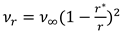
and the detectable frequency is
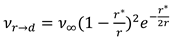
where, is the frequency of absorption line in that the light rays cross through a ring located at a position of , and is the absorption frequency case that structure would absorb in no-gravity fields. One can of course calculate the widths of absorption lines just like that of emission lines.
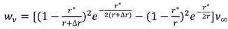
or
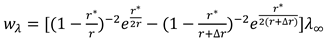
where, is absorption width of a ring that the light ray passes across.
or expressed by Doppler velocity in frequency as

or Doppler velocity in wave length as

But more different from emissions, absorption spectrums must have more narrow lines and lower redshift than emissions, because the absorption rings are mostly at outer regions with respect to the inner shining emission source, otherwise they would be difficult to be detected.
As we have discussed above, the inflow of inner rings of accretion may act as key role of entire emissions. So, we can image that brighter inner rings emit light rays, and on our view line, they go through some surrounding rings to be absorbed. It is said that, absorbing dusts might be the matters located at surrounding outer positions rather than those so called insert bodies far away from the emission areas. This image may lead to the so called relative blueshift, with respect to that of emission lines. Of course, there might be still seldom absorptions happening in inner areas so that we will also observe relative redshift absorption lines occasionally. Given a separation between emission position and absorption position more exterior, the emission frequency could be calculated as
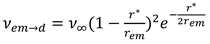
with redshift of the line
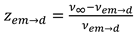
and absorption frequency varies because a separation between absorption and emission positions
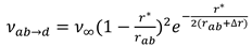
so that the redshift of absorption line is
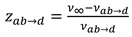
And then, there is a blueshift of an absorption line

Given and , it can be calculated that and 1.66. Here, the absorption lines may show a blueshift of with respect to the emission lines.
We have found that there were also absorption broad line region and absorption narrow line region [55] in single system in which those absorption lines were all corresponding to that of emission lines.
Case a continuum spectrum of light rays passes across multiple rings and arrive at an observatory on the Earth, one can then get a set of multiple frequency shift of absorptions. It is because absorptions only depend on position in accretions. This does interpret the multiple redshift absorption lines in tremendous of observations [48,49,54] on those active galactic nuclei. Especially for that of so called Lyman-alpha forest [56], a series of regular Lyman-alpha absorption lines, with descending order of redshifts, queue up amazingly at the left side of the great main emission line.
There is a special condition for a matter out flowing from center source, for example the center jet outflow. When a matter at ground state moves a separation toward outer direction, its structural energy should experience energy deficiency in that the energy of equivalent state gets increasing. We then see that the matter is in the state lack of energy, and generally, the state should be kept until surrounding environment happens to give amount of specific light sources, so as the result, the matter gets absorptions. It is said that, this kind of absorptions would be far different from normal relativistic absorptions as that have been discussed above, so that they could be called the super relativistic absorption. As for the mentioned absorption energy, it depends on the position it getting absorbing as well as the position it has ever been in ground state. Note that this kind of absorptions really distinguish from the general relativistic absorptions in that the super relativistic absorption energy depends on the difference between the final emission position and specific absorption position, while the general relativistic absorption is due to property of structure state. It could be calculated as
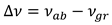
where, , , is the radius at absorption position, and is the radius of the position of equivalent ground state before outflow. This kind of absorption might need greater absorption energy than that of general relativistic absorption, and it does nothing with original absorption energy. Therefore, it should be called the super relativistic absorption.
To the observer at a farthest position, the absorption line will also perform special frequency shift that
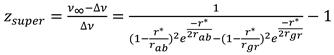
Case the jet flow particles of an active galactic nucleus are assigned in a broad area, it could cause a broader absorption pit for a crossing light ray. One can calculate the average redshift and the width of absorption pit.
Additionally speaking on the topic of jet flow, massive particles may be easily accelerated up and keep approaching absolute light speed so as to escape from inner event horizon. On the other hand, apparent light speed may be at lower level in the nearby area so that to form pseudo super luminal motions. A high pseudo super luminal motion may cause Cherenkov radiation, which could generally show polarized propagation. That might also be the reasons for some high energy light rays. One can imagine that the events of γ-ray burst detection delay in observations on SN1987A [57] and GW170817 [58] might be interpreted by pseudo super luminal propagations of neutrinos and gravitational waves.
Acknowledgements
Great many thanks to whom that I sent them emails for communications years ago early after part of the topics were developed. Thereafter, these researches have been completed in a very long time. I will appreciate anyone who are going to download and read this article in that it will be a hard work of weeks or longer to make complicated calculations and comprehensive understandings. And I will highly appreciate anyone who are going to feedback comments and peer reviews that may help for further communications.
References
- A. Einstein, Die Grundlage der allgemeinen Relativitätstheorie, Annalen der Phys., 49,769(1916). [CrossRef]
- J. Jost, Riemannian Geometry and Geometric Analysis, Springer –Verlag Berlin Heidelberg, Sixth Edition 2011, (1965).
- T. P. Cheng, Relativity, Gravitation,and Cosmology, Oxford University Press (2005).
- N. Straumann, General Relativity, Springer Science + Business Media Dordrecht( 2004, 2013).
- L. P. Eisenhart, Riemannian geometry, Princeton University Press, Eighth Printing 1997, (1925).
- П.К.Рашевский, Riemannian Geometry and Tensor Analysis, Technique and Theory Press, (1953).
- C. Huang, General Relativity Lecture Sheet, China Science Press (2023).
- A. Einstein, Zur Elektrodynamik bewegter Körper, Ann. Physik, 17,891(1905).
- H. Minkowski, Nachr. Ges. Wiss. Göttn Math.-Phys. Kl. 53 (1908).
- Y. Yu, General Relativity, Peking University Press (1997).
- H. Jin, Introduction to General Theory of Relativity, Zhejiang University Press (2022).
- B. Chen, General Relativity, Peking University Press (2018).
- C. E. Weatherburn, An Introduction to Riemannian Geometry and the Tensor Calculus, Cambridge University Press, (1942).
- R. Pound, G. Rebka, Gravitational Red-shift in Nuclear Resonance, Physical Review Letters. 3 (9): 439–441 (1959). [CrossRef]
- R. Vessot, M. Levine; E. Mattison et al., Test of Relativistic Gravitation with a Space-Borne Hydrogen Maser, Physical Review Letters. 45 (26): 2081–2084(1980). [CrossRef]
- T. Do, et al., Relativistic Redshift of the Star S0-2 Orbiting the Galactic Center Supermassive Black Hole, Science. 365 (6454) (2019). [CrossRef]
- S. Weinberg, Gravitation and Cosmology, Principles and Applications of the General Theory of Relativity, John Wiley (1972).
- R. Peierls, More Surprises in Theoretical Physics, Princeton Univ. Press (1991).
- H. Minkowski, Nachr. Ges. Wiss. Göttn Math.-Phys. Kl. 53 (1908).
- M. Abraham, Rend. Circ. Matem. Palermo 28, 1 (1909).
- A. Einstein, A centenary volume letter to M. Besso, 1951(p.138).
- U. Leonhardt, Optics: Momentum in an Uncertain Light, Nature, 444:823–824 (2006).
- M. Froeschle, F. Miguard, F. Arenon, in Proceedings of the Happarcos Venice 1997 Symposium, ESA Publications Division, Noordwijk (1997).
- I. I. Shapiro, Fourth Test of General Relativity. Physical Review Letters. 13 (26): 789–791 (1964). [CrossRef]
- I. I. Shapiro, M. E. Ash, R. P. Ingalls etc., Fourth Test of General Relativity: New Radar Result. Physical Review Letters. 26 (18): 1132–1135 (1971). [CrossRef]
- J. Roche, What is mass? European Journal of Physics, 26:1–18(2005). [CrossRef]
- Q, Xu, Z. Liu, Ordinary Differential Equations Analytical Methods and Numerical Methods, Publishing House of Electronics Industry, China (2022).
- B. B. Perera, M. A. McLaughlin, M. Kramer etc., The Evolution of PSR J0737-3039B and a Model for Relativistic Spin Precession, the Astrophysical Journal, 721: 1193-1205(2010). [CrossRef]
- P. Landry, B. Kumar, Constraints on the Moment of Inertia of PSR J0737-3039A from GW170817, arxive: 1807. 04727v2 [gr-qc] 10 Oct 2018. [CrossRef]
- C. W. F. Everitt etc., Gravity Probe B: Final Result of a Space Experiment to Text General Relativity, Phys. Rev. Lett., 106(22): 221101(2011). [CrossRef]
- R. Abuter, A. Amorim, N.Anugu etc., Detection of the Gravitational Redshift in the Orbit of the Star S2 Near the Galactic Centre Massive Black Hole, Astronomy & Astrophysics, 615, L15:1-10(2018). [CrossRef]
- J.H. Taylor, L.A. Fowler, and P.M. McCulloch, Measurements of General Relativistic Effects in the Binary Pulsar PSR1913+16, Nature, 277:437 (1978). [CrossRef]
- E. E. Salpeter, Accretion of interstellar matter by massive objects. Astrophys. J., 1964, 140, 796–800. [CrossRef]
- Y. B. Dovich, and I. D. Novikov, The radiation of gravity waves by bodies moving in the field of a collapsing star. Sov. Phys. Dokl., 9, 246 (1964).
- S. Kato, J. Fukue, S. Mineshige, Black-hole Accretion Disks, Kyoto University Press (2008).
- R. D. Blandford, H. Netzer, L. Woltjer, Active galactic nuclei, Saas-Fee Advanced Course 20,Lecture Notes 1990, Swiss Society for Astrophysics and Astronomy, Springer-Verlag Berlin Heidelber (1990).
- N. I. Shakura, R. A. Sunyaev, Black holes in binary systems. Observational appearance. Astron. Astrophys., 24, 337–355 (1973).
- S. L. Shapiro, A. P. Lightman, and D. M. Eardley: Astrophys. J. 204 187 (1976).
- B. Sicardy, Dynamics of planetary rings, Lect. Notes Phys. 682, 183–200 (2006).
- J. C. Maxwell, On the Stability of the Motions of Saturn’s Rings, Cambridge and London: MacMillan and Company. Reprinted in Scientific Papers of James Clerk Maxwell, Vol. 1, Cambridge University Press (1890).
- S. Charnoz, A. Croda, R. Hyodo, Rings in the Solar System: a Short Review, arxiv, 201805.08963 (2018).
- L. W. Esposito, Composition, Structure, Dynamics, and Evolution of Saturn’s Rings, Annu. Rev. Earth Planet. Sci. 38,383-410 (2010). [CrossRef]
- E. D. Miner, R. R. Wessen, J. N. Cuzzi, Planetary Ring Systems, Praxis Publishing Ltd, Chichester, UK (2007).
- B. Lee, R. Chary, Insights into Physical Conditions and Magnetic Fields from High Redshift Quasars, arxive: 2207. 07290v1 [astro-ph.GA] 15 Jul 2022.
- Event Horizon Telescope Collaboration, First M87 event horizon telescope results. I. The shadow of the supermassive black hole, ApJ, 875, L1, 17 (2019).
- C.T. Donnan, D.J. Mcleod, J.S. Dulop ect., The Evolution of the Galaxy UV Luninosity Function at Reshift z≈8-15 from Deep JWST and Ground-based Near-infrared Imaging, arxive: 2207. 12356v3 [astro-ph.GA] 24 Nov 2022.
- L.Y. Yung, R.S. Somerville, S.L. Finkelstein ect., Are the Ultra-high-redshift Galaxies at z>10 Surprising in the Context of Standard Galaxy Formation Models? arxive: 2304. 04348v2 [astro-ph.GA] 11 Nov 2023.
- V. Beckmann, Chris shrader, Active galactic nuclei, WILEY-VCH Verlag GmbH & Co. KGaA, Boschstr. 12, 69469, Weinheim, Germany (2012).
- K. Huang, Quasars and Active Galactic Nuclei, China Science and Technology Press, (2005).
- D. E. Osterbrock, Emission-line spectra and the nature of active galactic nuclei, proceedings of a conference held at the Georgia State University, Springer-Verlag, 1-18 (1987).
- M.C. Bentz, P.R. Williams, T. Treu, The Broad Line Region and Black Hole Mass of NGC 4151, arxive: 2206. 03513v1 [astro-ph.GA] 7 Jun 2022. [CrossRef]
- R. Serafinelli, A. Marinucci, A.D. Rosa etc., A Remarkably Stable Accretion Disk in the Sefert Galaxy, arxive: 2309. 06092v1 [astro-ph.HE] 12 Sep 2023.
- V. Liu, A. Zoghbi, J.M. Miller, Dectection of Asymmetry in the Narrow Fe Kα Line in MCG-5-23-16 with Chandra, arxive: 2312. 16354v2 [astro-ph.HE] 4 Jan 2024.
- B. M. Peterson, An introduction to active galactic nuclei, Cambridge University Press (1997).
- H. Netzer, The Physics and Evolution of Active Galactic Nuclei, Cambridge University Press (2013).
- R. Lynds, The Absorption-line spectrum of 4c 05.34, Astrophysical Journal, vol. 164, p.L73 (1971). [CrossRef]
- K. Hirata et al., Observation of a Neutrino Burst from the Supernova SN1987a, Phys. Rev. Lett., 58:1490-1493(1987). [CrossRef]
- B. P. Abbott et al., GW170817: Observation of Gravitational Waves from a Binary Neutron Star Inspiral, Phys. Rev. Lett., 119:161101(2017). [CrossRef]
Figure 1.
Center source field.
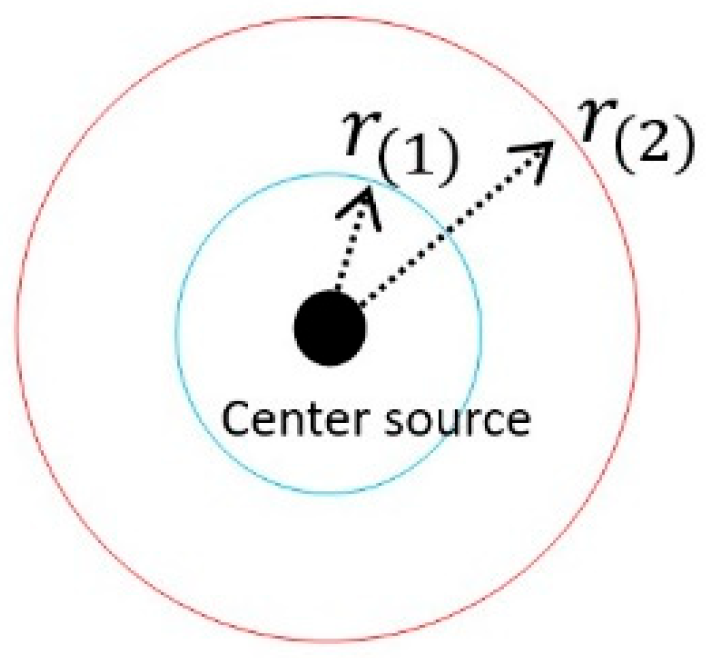
Figure 2.
World lines for a pulse of photons.
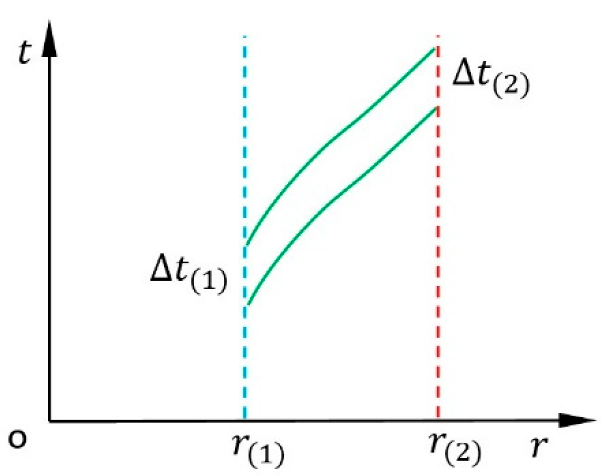
Figure 3.
A super surface as covariant space in 3-dimensional space.
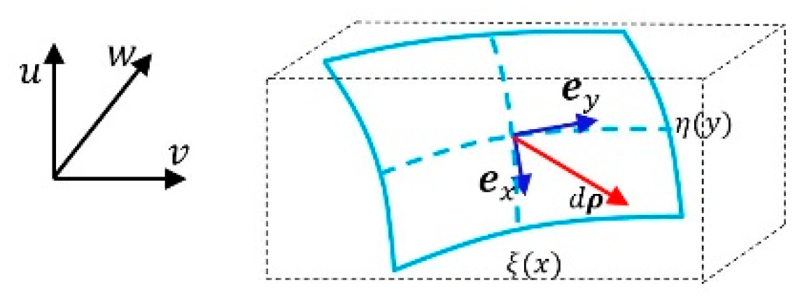
Figure 4.
A coordinate plane as contra variant space in 3-dimensional space.
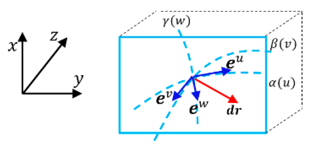
Figure 5.
Covariant tangent space .
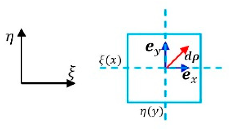
Figure 6.
Contra variant tangent space.
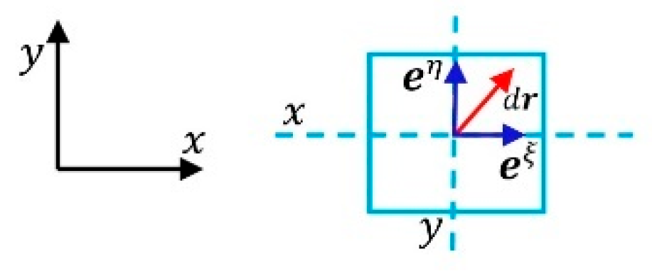
Figure 7.
Covariant space.
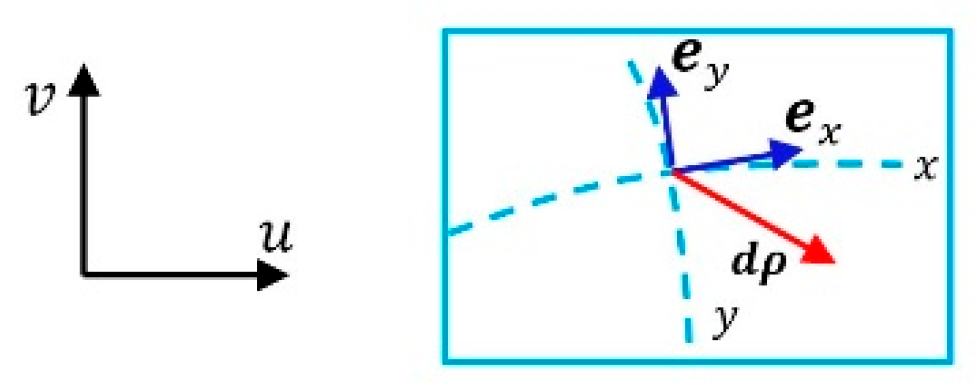
Figure 8.
Contra variant space.
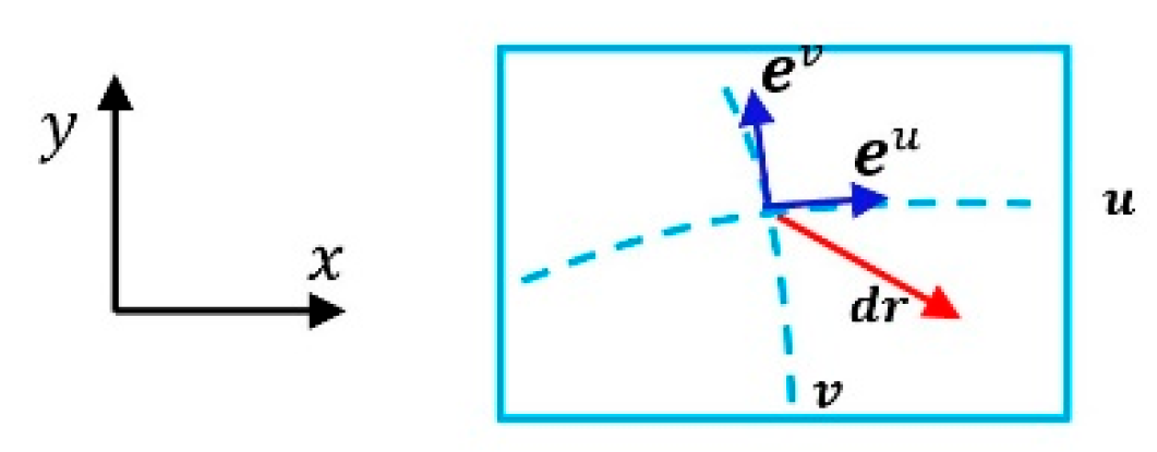
Figure 9.
Bases vary in different paths.
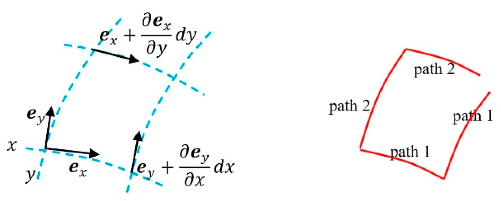
Figure 10.
Covariant space.
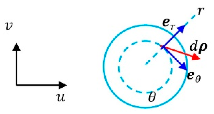
Figure 11.
Contra variant space.
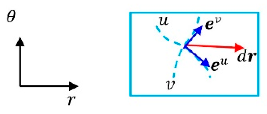
Figure 12.
Covariant space.
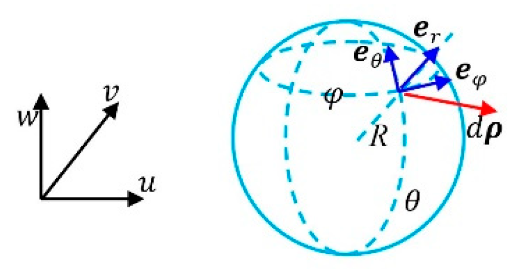
Figure 13.
Contra variant space.
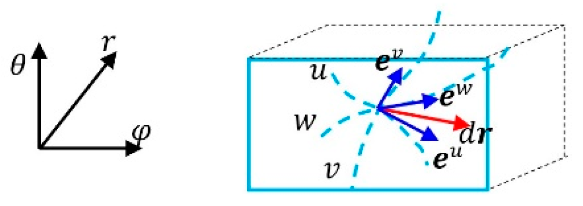
Figure 14.
Covariant spac.
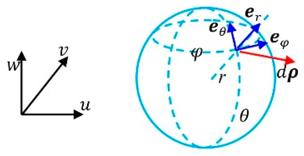
Figure 15.
Contra variant space.
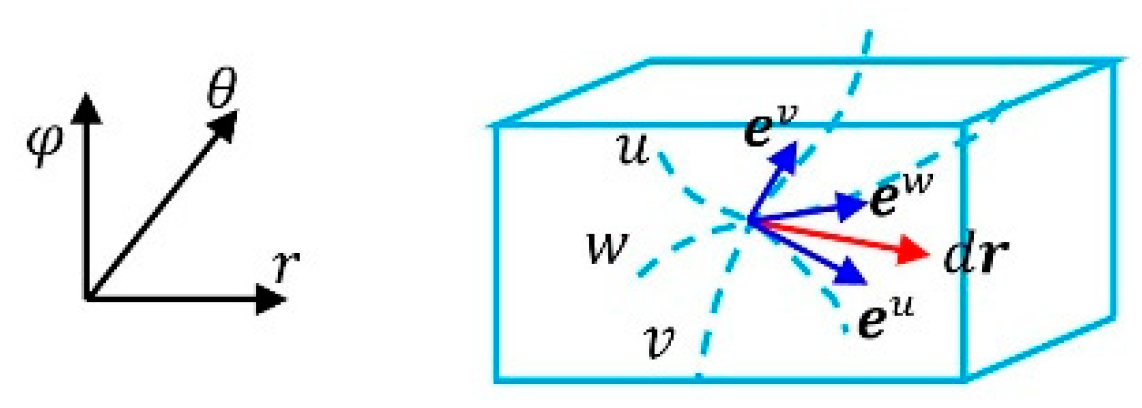
Figure 16.
A photon traveling in center source field.
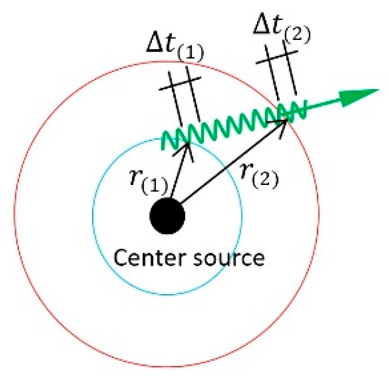
Figure 17.
Free falling measurement.
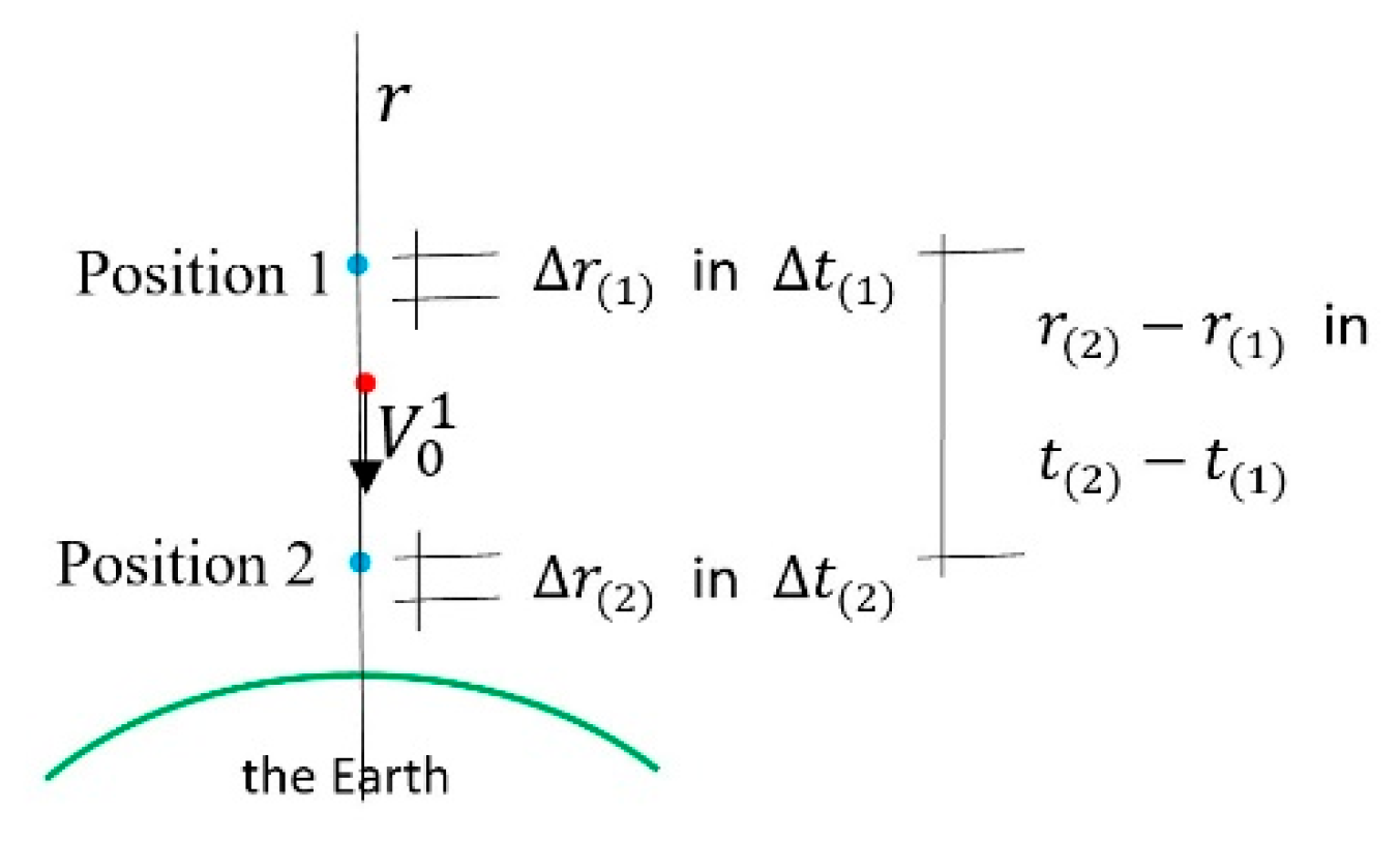
Figure 18.
Light rays passing across the Sun.
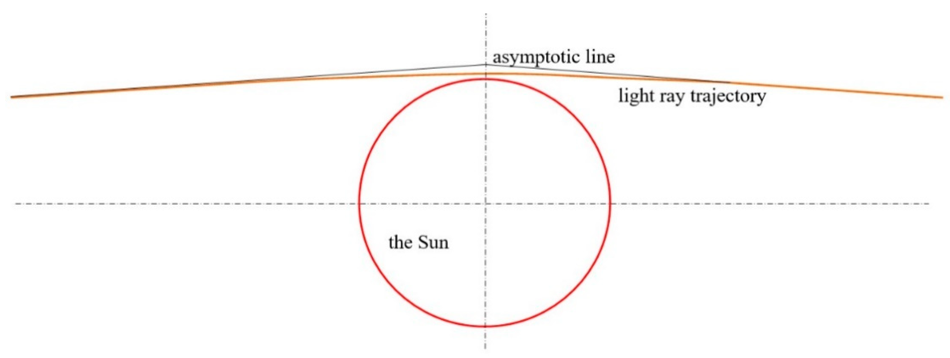
Figure 19.
Detailed relationships for angles of light rays and view lines and coordinates.
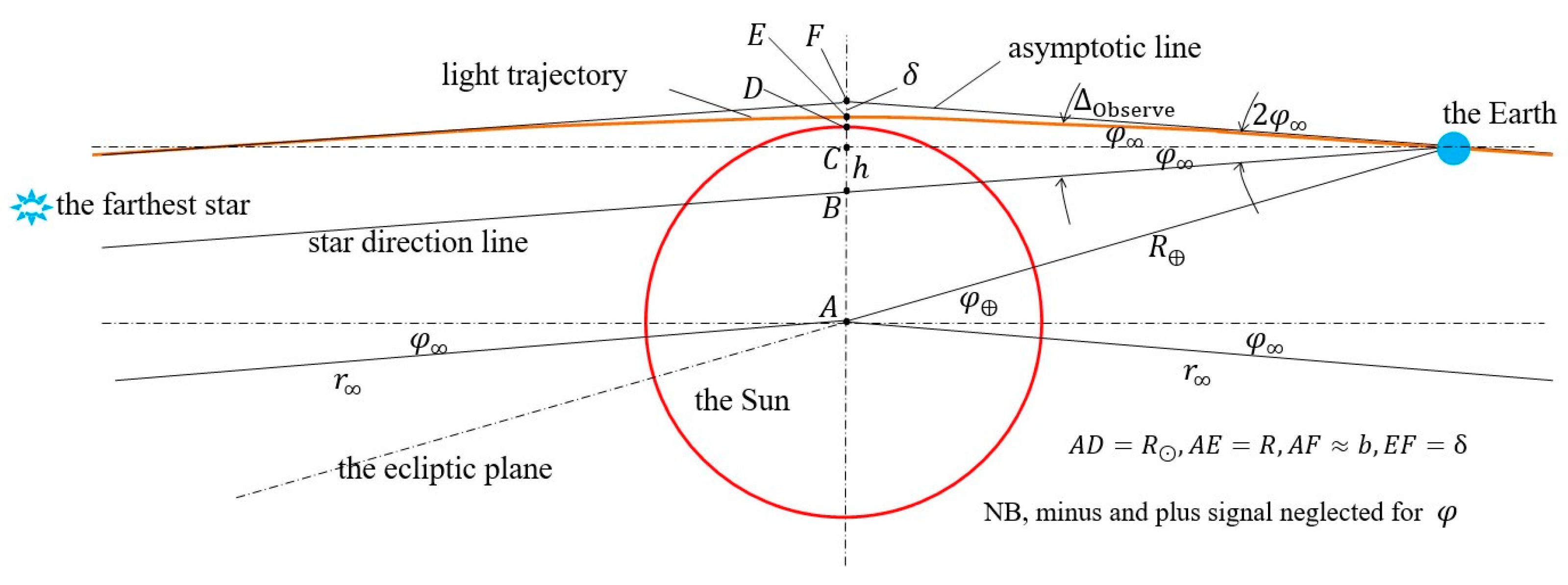
Figure 20.
Asymptotic line with an overplayed
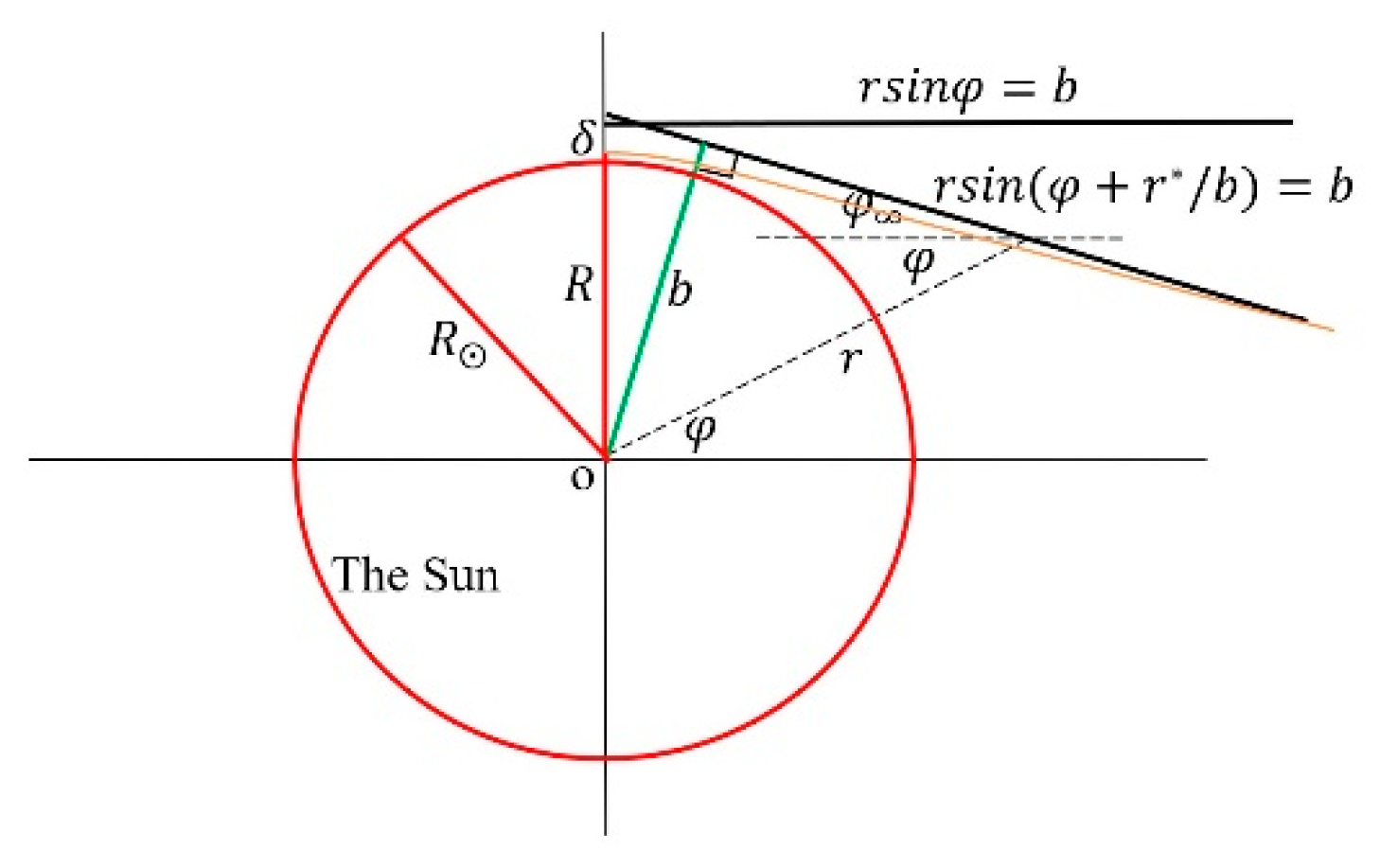
Figure 21.
Invalidity of Newtonian second law for light deviation.
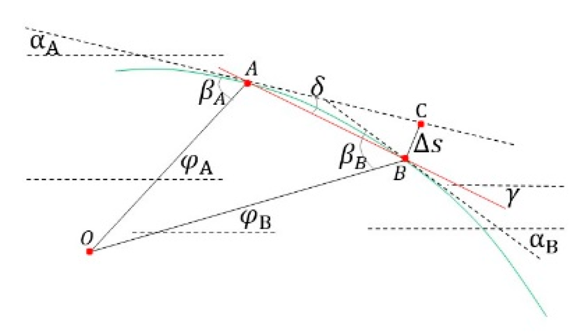
Figure 22.
Probability of ballistic trajectory method for light deviation.
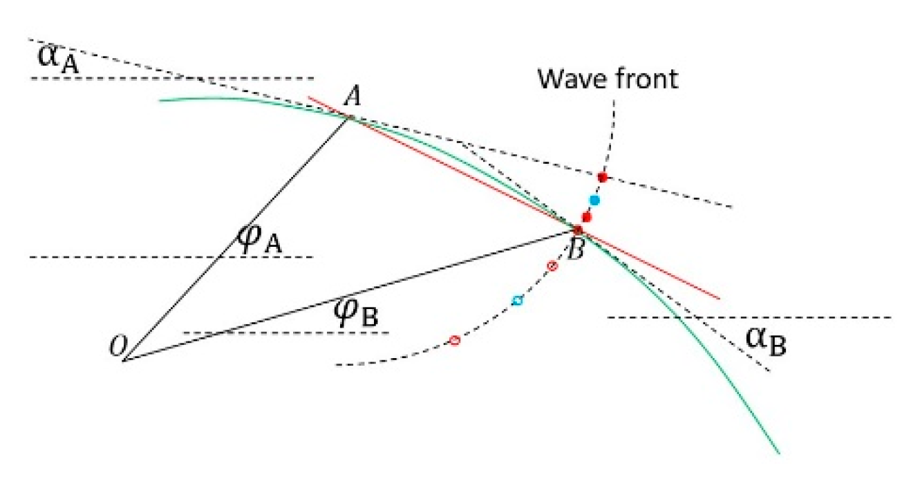
Figure 23.
Fluid ring in one source field.
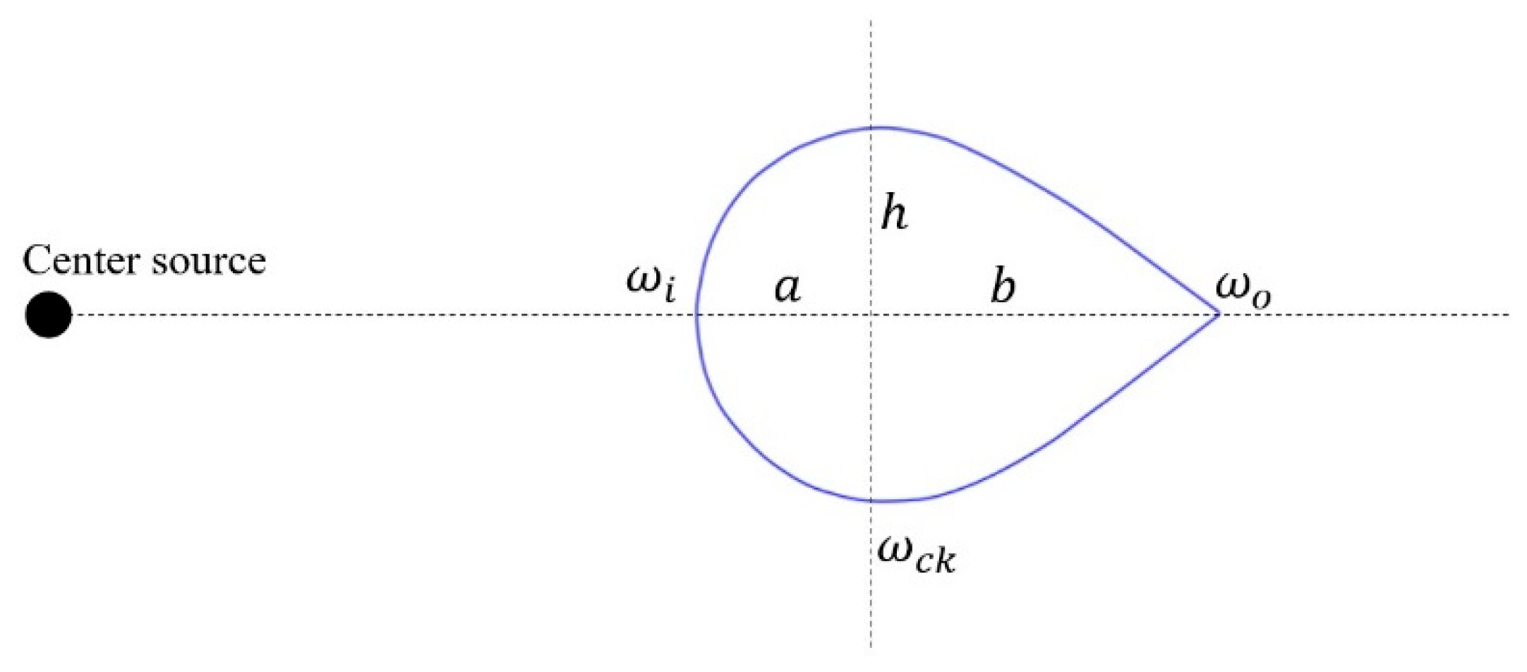
Figure 24.
Angular momentum conversion between neighboring rings.

Table 1.
Base components , derivatives and gravity at experimental positions.
| 6372.393 | 1.00000000069582045 | 0.99999999930417955 | 9.81377376 | 2.183859184×10⁻¹⁶ |
| 6371.493 | 1.00000000069591874 | 0.99999999930408126 | 9.81654643 | 2.184476187×10⁻¹⁶ |
| 6371.393 | 1.00000000069592966 | 0.99999999930407034 | 9.81685457 | 2.184544758×10⁻¹⁶ |
Table 2.
Terrestrial freefalling experiments from position 6371.493 to 6371.393.
| Analysis method | Theoretical analysis | Measurable analysis | ||||
| Positions | r(1)=6371.493 | r(2)=6371.393 | From r(1) to r(2) | |||
| Initial velocity | Contra variant acceleration |
Covariant acceleration |
Contra variant acceleration |
Covariant acceleration |
measured time intervals |
Covariant acceleration |
| (m/s) | (m/s2) | (m/s2) | (m/s2) | (m/s2) | (s) | (m/s2) |
| 0 | 9.8165464 | 9.8165464 | 9.8168546 | 9.8168546 | 4.5137 | 9.8165 |
| 100000 | 9.8165453 | 9.8165453 | 9.8168535 | 9.8168535 | 1.0×10⁻³ | 9.8165 |
| 10000000 | 9.8056240 | 9.8058425 | 9.8059318 | 9.8061503 | 1.0×10⁻⁵ | 9.8275 |
| 100000000 | 8.7243083 | 10.908784 | 8.7245822 | 10.909127 | 1.0×10⁻⁶ | 10.908 |
| 200000000 | 5.4475940 | 14.185499 | 5.4477651 | 14.185944 | 5.0×10⁻⁷ | 14.184 |
| 250000000 | 2.9900583 | 16.643034 | 2.9901522 | 16.643557 | 4.0×10⁻⁷ | 16.640 |
| 299792458 | 0 | 19.633093 | 0 | 19.633709 | 3.3356×10⁻⁷ | 19.629 |
Table 3.
Terrestrial freefalling experiments from position 6372.393 to 6371.393.
| Analysis method | Theoretical analysis | Measurable analysis | ||||
| Positions | r(1)=6372.393 | r(2)=6371.393 | From r(1) to r(2) | |||
| Initial velocity | Contra variant acceleration |
Covariant acceleration |
Contra variant acceleration |
Covariant acceleration |
measured time intervals |
Covariant acceleration |
| (m/s) | (m/s2) | (m/s2) | (m/s2) | (m/s2) | (s) | (m/s2) |
| 0 | 9.8137738 | 9.8137738 | 9.8168546 | 9.8168546 | 14.276 | 9.8138 |
| 100000 | 9.8137730 | 9.8137751 | 9.8168535 | 9.8168535 | 1.0×10⁻² | 9.8138 |
| 10000000 | 9.8028548 | 9.8246934 | 9.8059318 | 9.8061503 | 1.0×10⁻⁴ | 9.8247 |
| 100000000 | 8.7218446 | 10.905704 | 8.7245822 | 10.909127 | 1.0×10⁻⁵ | 10.906 |
| 200000000 | 5.4460559 | 14.181493 | 5.4477651 | 14.185944 | 5.0×10⁻⁶ | 14.182 |
| 250000000 | 2.9892144 | 16.383343 | 2.9901522 | 16.643557 | 4.0×10⁻⁶ | 16.639 |
| 299792458 | 0 | 19.627547 | 0 | 19.633709 | 3.3356×10⁻⁶ | 19.629 |
Table 4.
Relativistic and detectable frequency shifts at different positions.
| Emission positions | Relativistic frequency shifts | Detectable frequency shifts |
| 17.778 | 26.585 | |
| 11.250 | 16.508 | |
| 8.000 | 11.561 | |
| 3.000 | 4.136 | |
| 1.250 | 1.658 | |
| 0.235 | 0.298 | |
| 0.108 | 0.136 |
Table 5.
Emission line widths at different positions with specific exciting widths.
| Emission positions | Exciting widths | km/s | km/s | ||
| 0.02327 | 87681 | 2.8408 | 67850 | ||
| 0.01158 | 43634 | 1.5949 | 38093 | ||
| 0.01433 | 11425 | 0.09752 | 11006 | ||
| 0.007239 | 5772 | 0.05018 | 5663 | ||
| 0.002079 | 809 | 0.003492 | 807 | ||
| 0.001044 | 406 | 0.001756 | 406 | ||
| 0.0005706 | 194 | 0.0007360 | 194 | ||
| 0.0002860 | 97 | 0.0003690 | 97 | ||
| 0.00002455 | 7.6 | 0.00002582 | 7.6 | ||
| 0.00001228 | 3.8 | 0.00001291 | 3.8 |
Disclaimer/Publisher’s Note: The statements, opinions and data contained in all publications are solely those of the individual author(s) and contributor(s) and not of MDPI and/or the editor(s). MDPI and/or the editor(s) disclaim responsibility for any injury to people or property resulting from any ideas, methods, instructions or products referred to in the content. |
© 2025 by the authors. Licensee MDPI, Basel, Switzerland. This article is an open access article distributed under the terms and conditions of the Creative Commons Attribution (CC BY) license (http://creativecommons.org/licenses/by/4.0/).
Copyright: This open access article is published under a Creative Commons CC BY 4.0 license, which permit the free download, distribution, and reuse, provided that the author and preprint are cited in any reuse.


