
Submitted:
08 May 2025
Posted:
09 May 2025
You are already at the latest version
Abstract
The characteristic structure of the two-dimensional adjoint Euler equations is examined. The characteristic behaviour is similar to that of the original Euler equations, but with the characteristic information travelling in the opposite direction. The compatibility conditions obeyed by the adjoint variables along characteristic lines are derived. It is also shown that adjoint variables can have discontinuities across characteristics and the corresponding jump conditions are obtained. It is shown how this information can be used to obtain exact predictions for the adjoint variables, particularly for supersonic flows. The approach is illustrated by the analysis of supersonic flow past a double wedge airfoil, for which an analytic adjoint solution is obtained in the near-wall region.
Keywords:
adjoint variables
; compressible flow
; characteristic lines
; compatibility conditions
; supersonic flow
; Mach lines
; Riemann invariants
; jump conditions
; shock-expansion theory
; aerodynamic design
1. Introduction
This paper considers the characteristic structure of the adjoint Euler equations [1] with particular emphasis in supersonic flow, where the adjoint approach has been applied to a wide variety of problems ranging from general-purpose aerodynamic shape design [2,3], sonic boom mitigation [4,5,6,7], flow control [9], anisotropic grid adaptation [9], etc. For simplicity, the analysis is restricted to two dimensional flows. Steady inviscid compressible flow in two dimensions obeys the Euler equations
where
In eq. (2), are the Cartesian components of the velocity, is the density, p is the pressure and E and H are the total energy and enthalpy, respectively. For a perfect gas,
and
where is the modulus of the velocity and is the ratio of specific heats. The flow equations (1) can be written in quasi-linear form
where are the inviscid flux Jacobian matrices. Eq. (5) is the starting point for the characteristic analysis of the Euler equations as we will show momentarily.
The derivation of the adjoint Euler equations is quite standard (see, for example, [1,10,11,12]) and will not be repeated here. For definiteness, we will focus on an external aerodynamics problem consisting on an airfoil with profile S immersed in a flow with incidence . For this case, we wish to compute the sensitivities of a cost function measuring aerodynamic drag given as the integral of the pressure along a wall boundary S
where is a normalization constant, is a reference length – the chord length of the airfoil, is the wall unit normal vector and lies along the inflow direction. The adjoint equations are
where are the adjoint variables. The adjoint boundary conditions are chosen to eliminate the integral of on the boundaries. This procedure results in dual characteristic boundary conditions (obtained from a locally one-dimensional characteristic decomposition) in the far-field [1,10,11], while at the wall the adjoint variables obey
The characteristic structure of eq. (5) is well known and depends on the local Mach number M [13]. For subsonic flow, there is only one family of characteristic lines (the streamlines), while for supersonic flows there are two additional families of characteristics, the Mach lines that are inclined at an angle to the local flow direction. Along characteristics, the partial differential equations (PDE) that describe the flow reduce to ordinary differential equations (ODE) called compatibility equations. In certain circumstances, notably in the case of two-dimensional irrotational supersonic flow, the compatibility conditions can be integrated and are further reduced to algebraic equations that hold only along the characteristic lines. The information carried by the compatibility conditions can be used to simplify the computation of supersonic flows, one notable practical application being the design of supersonic nozzles [13].
The adjoint equations (7) share the same characteristic structure as the flow equations but with the sign of each characteristic velocity reversed so that the characteristic information travels in the opposite direction [1,12]. As in the previous case, the adjoint variables obey compatibility conditions along the characteristics (see e.g. [14] and references therein). In the recent works [15,16], the flow and adjoint compatibility conditions were obtained and checked on several numerical adjoint solutions.
The adjoint equations are linear and, for supersonic flows, hyperbolic. As a result of this, the behavior of the analytic supersonic adjoint solutions is strongly constrained by the characteristic structure of the equations. On the one hand, and barring special cases where cost functions are defined along certain lines, not necessarily characteristic, such as in [4], the adjoint variables can only have discontinuities along characteristic lines. The jumps in the adjoint variables along these lines are constrained by jump conditions as will be shown in section 2. Additionally, as in supersonic flow information travels along characteristic lines, supersonic adjoint solutions tend to follow characteristic lines emanating from significant features of the flow or the geometry such as leading and trailing edges, shock feet, etc. as shown in, e.g., [14,15,16,17,18,1920] and in section 3. This is significant as it is precisely in those regions, where the amplitude of the adjoint solution is usually highest, that the cost function is most sensitive to perturbations.
In this paper, we review the characteristic structure of the adjoint Euler equations and obtain the corresponding compatibility and jump conditions along and across characteristic lines and show how this information can be used to obtain quantitative predictions for the adjoint variables by considering supersonic past a diamond airfoil, for which a closed-form analytic adjoint solution, valid in the near wall region, is presented and checked against a numerical adjoint solution on a very fine grid.
2. Characteristic Structure of the Adjoint Euler Equations
This section contains a brief analysis of the characteristic structure of the flow and adjoint Euler equations. We also refer the reader to the recent works [15,16], where a similar analysis is carried out.
2.1. Compatibility Conditions: Reduction of the PDE to an ODE
Both the 2D steady flow and adjoint Euler equations (5) and (7) are written in quasilinear form,
For a general quasilinear system (9), its characteristic structure is determined by the solution of the eigenvalue problem [21]
Notice that, since , it is clear that the characteristic structure of the flow and adjoint equations is identical.
If is a real solution of eq. (10), then the planar curve with local slope
is a characteristic curve of the above quasilinear system. Across characteristics, both the solution and its first derivatives may be discontinuous. Furthermore, the original system of equations can be reduced to an ODE along characteristics. Such ODES, one per characteristic curve, are called compatibility conditions, and can be obtained as follows.
Suppose is a real eigenvalue of . The matrix is singular, so there exists a left eigenvector lλ such that
Multiplying eq. (9) on the left by lλ and using the properties of the left eigenvector yields a scalar equation
In eq. (13),
is (proportional to) the (tangent) derivative along the characteristic curve with local slope λ = dy/dx, so the scalar ODE (13) reduces to
Eq. (15) is the compatibility condition obeyed along the characteristic line by the solution to the PDE. There is one such compatibility condition along each of the families of characteristics. Besides, if the compatibility condition is integrable, it can be rearranged into the generic form
where , which is conserved along the characteristics λ = dy/dx, is called a Riemann invariant.
All the above translates immediately to the Euler equations. The adjoint equations, however, are transposed, so a bit of additional work is required. To obtain the adjoint compatibility conditions we consider again the eigenvalue problem , where . For real one can define, in addition to the left eigenvector, a right eigenvector such that
Multiplying the adjoint equation on the left by and using yields the adjoint compatibility condition
Under generic circumstances, it is unlikely that the adjoint compatibility conditions can be integrated. However, if the coefficients are constant along a certain characteristic line or in regions of constant flow, the quantities (that we will call Riemann functions in what follows) are Riemann invariants for the adjoint equations along λ characteristics.
2.2. Discontinuities Across Characteristics: Jump Conditions
Across characteristics, both the solution and its first derivatives may be discontinuous [21], but the structure of the equations impose matching or jump conditions on the solution and its derivatives. Let us consider a characteristic line associated to the real eigenvalue. We assume that the Jacobian matrices (A,B) are continuous (the case of discontinuous Jacobians corresponds to shocks or slip lines that have a singular treatment of their own [22,23,24] and will not be further considered here) and distinguish two cases depending on whether is continuous or not.
If is continuous, the tangent derivatives across the characteristic line are also continuous and, by decomposing the equation in a local tangent and normal frame relative to the characteristic and taking differences across the characteristic line we get
where is the normal vector to the characteristic line.
On the other hand, if is discontinuous across the characteristic line, its behavior across the discontinuity is given by the following jump conditions [21]
The proof of eq. (20) is identical to that of the Rankine-Hugoniot conditions for shocks, involving the integration of the adjoint equation against a test function on a suitably chosen domain divided in two by the line of discontinuity.
Eq. (20) is equivalent to , so the jump in the adjoint variables across a characteristic line must be a left eigenvector of .
Notice that, in either eqs. (19) and (20), the coefficient matrix of the linear system is not invertible along the characteristic, so the above equations admit non-trivial solutions. Conversely, if the line is not characteristic, then neither eqs. (19) nor (20) admit non-trivial solutions.
2.3. Relation of Jumps Across Characteristic Lines and Compatibility Conditions
The jump conditions give a series of linear combinations of adjoint variables that are continuous across the characteristic line. Of course, not all of these are linearly independent (otherwise, the adjoint variables would be continuous across the characteristic). In fact, has rank n − k, where n is the number of equations and k is the multiplicity of the eigenvalue. This can be understood with the following result, which also sheds light onto the jump conditions. Pick a characteristic line with eigenvalue and multiplicity ki. The corresponding jump conditions are
Now multiply (21) on the left by the right eigenvector corresponding to one of the n − ki remaining eigenvalues,
Now, since , the jump conditions can be written as
for j ≠ i. Now recall that along a characteristic j, the adjoint variables obey the compatibility condition , from where we can define the Riemann functions (which turn out to be Riemann invariants along the j characteristic under particular circumstances). We thus see that the jump conditions across one characteristic line are equivalent to the statement that the Riemann functions associated to characteristic lines that cross the given characteristic are continuous.
2.4. Characteristic Lines and Compatibility Conditions for the Adjoint Euler Equations
For the 2D Euler equations, the characteristic equation (10) has the following solutions [13]:
(double) and
where is the speed of sound, and is the local Mach number. The characteristic lines corresponding to λ0 are the flow streamlines. The associated compatibility conditions (15) can be arranged in the following form
(here represents variation along the characteristic line) which simply say that the enthalpy and entropy are constant along streamlines (even though they might vary from streamline to streamline).
On the other hand, are only real for supersonic flow, in which case the associated characteristic lines are, respectively, left (upper) and right (lower) -running Mach lines inclined at an angle relative to the local streamline. The corresponding compatibility conditions are
For irrotational flow, eq. (27) is equivalent to
where is the angle that the local streamline makes with the x axis. Eq. (28) can be integrated to give the Riemann invariants
where is the Prandtl-Meyer function [13].
For the adjoint equations, we have the exact same eigenvalues and characteristic lines, and the associated compatibility conditions can be obtained with the aid of an algebraic manipulation software (we have used Wolfgram Research’s Mathematica) and can be arranged in the following form
For homentropic flows, the compatibility conditions can be written as
The first compatibility condition in (30) can be immediately integrated, yielding the adjoint Riemann invariant , which is known to be constant along streamlines (and everywhere for cost functions that only depend on the pressure [12]). Furthermore, in supersonic regions where the flow variables are constant, the above compatibility conditions give rise to 4 adjoint Riemann invariants
along streamlines,
along right-running characteristics C− (with eigenvalue ) and
along left-running characteristics C+ (with eigenvalue ).
Even when they are not truly invariant, these Riemann functions have an additional interpretation as the adjoint variables corresponding to the flow compatibility conditions since
Hence, are related to perturbations along streamlines, while are related to perturbations along Mach lines. We will use this insight in the next section when we analyze a particular example.
One last application of the Riemann functions concerns the jump conditions across characteristics. Across characteristic lines the adjoint solution can jump. When it does, the jumps are subject to the conditions (20). The matrix has rank 2 for streamlines and rank 3 for Mach lines. So for a streamline, there are 2 independent jump conditions, which correspond to the continuity of the Riemann functions , while for a Mach line (resp. ) the 3 linearly independent jump conditions can be written in terms of the Riemann functions and and (resp. ), which is the Riemann function corresponding to the other Mach line.
3. Application of the Jump Conditions to a Supersonic case: Flow Past a Diamond Airfoil
The method of characteristics can be used to solve for the flowfield in the case of steady, supersonic flow, and can be applied to the design of supersonic nozzles for 2D shock-free, isentropic flow [13], since in that case the non-linear flow equations reduce to algebraic equations along the characteristic lines. Since adjoint compatibility conditions cannot be integrated in general, there is little hope that a similar approach can be used with the adjoint equations. However, it turns out that the characteristic structure of the equations can be used to obtain analytic results in particular cases. One such example is given by the supersonic flow past a double wedge (diamond shaped) airfoil.
We consider inviscid supersonic flow over a symmetric diamond airfoil, with chord length of one, and a thickness of 0.06 (resulting in a half-angle of τ = 6.85 deg). The free-stream Mach number is M∞ = 2 and the angle of attack (AOA) is 0 degrees. The flow contains two sets of wedge-shaped oblique shocks attached to the leading and trailing edges, and two expansion fans emanating at the mid-chord vertices (Figure 1).
The flow solution can be computed exactly using shock-expansion theory [13]. The flow is parallel to the free stream upstream of the leading edge shock and downstream of the trailing edge “fishtail” shock. Between the leading edge shock and the leading Mach line of the expansion fan, the flow is parallel to the front segment of the airfoil, with a Mach number M1 < M∞ that depends on the free stream Mach number and the wedge angle τ, which also determine the shock inclination. The flow then turns across the expansion fan (with limit Mach numbers M1 and M2) so that behind the trailing Mach line of the fan the flow is parallel to the rear segment of the airfoil until it reaches the fishtail shock. The Mach number along the rear section M2 > M∞ is determined by M1 and the turning angle 2τ. Finally, the wedge angle, M2 and M∞ determine the fishtail shock inclination. From shock-expansion theory, M1 ≈ 1.755 and M2 ≈ 2.254, which are in very good agreement with the numerical solution shown in Figure 2, computed with DLR’s Tau solver [25] on an unstructured mesh with over 8.2 million nodes and 5300 nodes on the airfoil profile, with an outer freestream boundary domain of around 50 chord lengths from the geometry.
The corresponding drag-based adjoint solution computed with Tau’s discrete adjoint solver is shown in Figure 3. The adjoint variables are non-dimensionalized relative to Tau’s reference values .
Figure 3 depicts the numerical adjoint solution along with the shocks and several notable characteristic lines (various streamlines, which are the nearly horizontal lines, as well as several Mach lines –the diagonal lines–, including the limits of the expansion fan and two Mach lines emanating from the trailing edge and running diagonally towards the upcoming flow). We see that the adjoint solution clearly follows the characteristic structure of the flow in a pattern that somehow mirrors that of the primal flow. The adjoint solution vanishes downstream of the two Mach lines impinging on the trailing edge since no perturbation past those lines can affect the flow about the airfoil. The solution is essentially concentrated along strips limited by Mach lines emanating from the trailing edge, the midchord vertices and the leading edge, and the adjoint solution is discontinuous along these characteristic lines. There is also a weak horizontal strip along the incoming stagnation streamline upstream of the forward shock, in agreement with the general structure described in [19]. Finally, the solution along the wall is piece-wise constant (see Figure 4), and it is actually possible to use the jump conditions (20) and the wall boundary condition to predict the values of the adjoint variables.
In this particular case, we start from the trailing edge and focus on the upper side. The right-moving Mach line emanating from the trailing edge separates two regions where the flow and the adjoint solutions are constant. Hence, the Riemann functions are piecewise constant, and the only one that can jump is the one associated to that characteristic line. The other 3 are continuous across the line and, being constant on either side, maintain the zero value that they have downstream of the Mach line. Hence, the adjoint variables upstream of the Mach line obey the equations
as well as the wall boundary condition eq. (8), which on the rearmost upper segment is simply . It is now easy to see that the above equations yield for the adjoint variables in the rearmost segment of the wall the following result
where and c2 and H2 are the speed of sound and total enthalpy at the rear part of the airfoil. Eq. (37) also holds on the lower side with the opposite sign for . This analytic solution is compared with the numerical solution in Figure 4, showing excellent agreement.
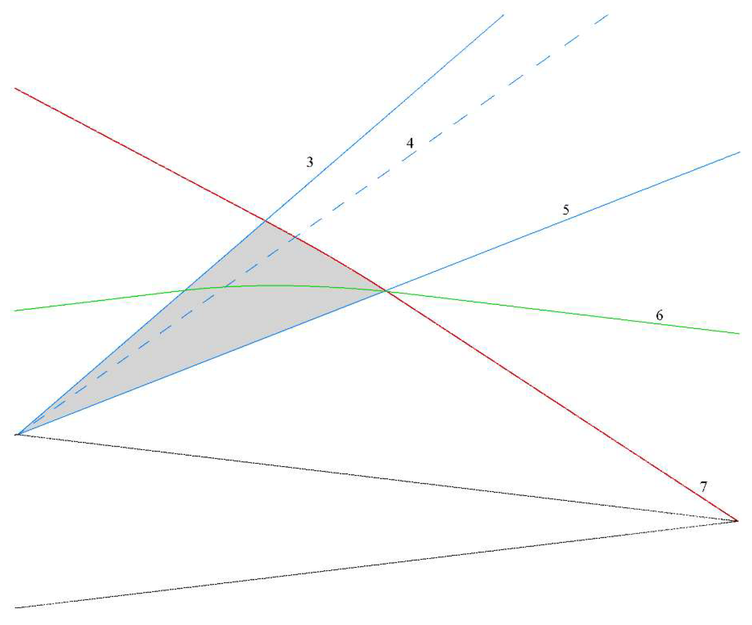
We see in Figure 4 that the adjoint solution along the wall is piecewise constant, with the values corresponding to the rear segment of the airfoil given by eq. (37). Away from the wall, the adjoint solution exhibits a fairly simple structure, at least in the immediate proximity of the wall, as can be seen in Figure 5 where the adjoint solution along a streamline is depicted and compared with the solution along the wall. The solution is again piecewise constant, and 5 plateaus can be clearly identified, which are separated by jumps across characteristic lines. The adjoint variable is zero (V) beyond the right-running Mach line emanating from the trailing edge (7). Then it stays constant (IV) until the fan (III), delimited by Mach lines (3) and (5), where it has a continuous variation. It achieves a second plateau (II), which does not appear in the wall solution, and then jumps again across the right-running Mach line (2) emanating from the vertex of the fan [14,17]. Finally, it jumps again across the right-running Mach line emanating from the leading edge (1). Notice that the plateau values I and IV agree fairly well with the wall values, which means that the adjoint solution is roughly constant throughout the corresponding regions.
It is also interesting to note that the Riemann function (34), associated to left-running characteristics, is constant (and in fact vanishes) throughout the upper side of the airfoil. In fact, it is only non-zero in the region of the pressure side of the airfoil limited by the left-running characteristics emanating from the leading and trailing edges – see Figure 6. The reason for this behavior can be found in the interpretation of the adjoint Riemann functions as adjoint variables to the flow compatibility conditions. is the adjoint variable associated to left-running characteristics, and it is only non-zero in the region of the fluid domain where perturbations carried by left-running characteristics can reach the airfoil and, thus have an impact on the cost function.
We can use this information to extend the analytic solution to the forward part of the airfoil. We start by recalling Giles and Pierce’s Green’s function approach [22], which allows to write any 2D inviscid adjoint solution in the generic form
where pt is the total pressure (which is constant between the leading and trailing shocks) and Ij, at any given point with coordinates , are the linearized cost functions corresponding to 4 linearly independent point source perturbations (mass, force normal to the flow direction, enthalpy and total pressure) [12] inserted at . For cost functions that only depend on pressure, I3 = 0 (total enthalpy perturbation at constant pressure), while requires that . Using this in eq. (38) and rearranging, yields
This is the general analytic solution. It depends on two functions and , whose values, for the numerical solution, are depicted in Figure 7.
In the extreme zones I and IV, is constant and its value is related to the adjoint wall boundary condition
where is the unit wall normal vector pointing towards the fluid, yielding
and
respectively. Within the expansion fan (zone III) we have non-constant, homentropic flow, so along right-running characteristics eq. (31) applies. Using also , and , where , we can obtain that
where is a constant. From eq. (43), we can obtain the (constant) value in zone II as
Lastly, in zone IV, , which fixes as
We now turn to . In zones I, II and IV, is constant, and actually since across the right-running Mach line emanating from the trailing edge and downstream. We can obtain further information by using the jump conditions across the right-running characteristic emanating from the midchord vertex to relate the solutions in zones I and II. In terms of the Riemann functions, the jump conditions are
The first and third equations in (46) are directly obeyed by the solutions on each side by construction, so we only have the middle condition
which yields and, thus , in agreement with Figure 7Across the expansion fan, changes between and . To obtain the value of across the fan we recall that is the effect on drag of a point perturbation to the stagnation pressure at constant static pressure [12]. Its value at a point is given by the integration along the local streamline of secondary sources of mass and force normal to the local flow direction [26,27]
In eq. (48), is the total density and the integral is taken from (s = 0) to the downstream farfield along the local streamline through . Let us consider a point inside the expansion fan. Firstly, the contribution to the integral vanishes downstream of the trailing Mach line of the fan. Secondly, the flow is isentropic, so the following relations hold along any streamline:
Furthermore, inside the fan the flow variables are constant along left-running Mach lines, so we have
(here μ is the Mach angle). Gathering eq. (48) – (50) and using we get
where is given by eq. (43) and we have changed the variable of integration to , which is the angle that the local left-running Mach line makes with the x axis and is the corresponding value for the final Mach line of the fan. The final piece of information required to evaluate eq. (51) comes from the analytic solution for the expansion fan [28]
where
Differentiating eq. (52) with respect to yields
Gathering all the information, we can write the analytic adjoint solutions as
in zone I, where gives the inclination of the fan’s leading Mach line relative to the x axis,
in zone II,
across the fan and
in zone IV, in agreement with eq. (37). The analytic solution eq. (55) – (58) is in remarkable agreement with the numerical solution as shown in Figure 4 and Figure 8.
Solution Across the Expansion Fan
Eq. (57) gives the spatially varying solution throughout the fan. Notice that, as is clear from eq. (57), the adjoint solution, like the flow solution, remains constant along each Mach line of the fan, as can be confirmed with the numerical solution in Figure 9, which depicts I2 and I4 and the adjoint variables along 3 Mach lines of the fan (roughly corresponding to the leading and trailing lines of the fan and a third interior line). The corresponding analytic values for I2 and I4 computed with eq. (43) and (51) are also shown for comparison, showing and excellent agreement.
We see that towards the center of the fan (located at x = 0.5 in the plot), I2 and I4 and the adjoint variables attain a constant value along each line of the fan, the value changing from line to line. I2 and I4 behave differently in this regard, since the former jumps abruptly across the right-running Mach line (7), while the latter shows a smooth variation and reaches a plateau at the intersection with the limiting streamline (6). The reason for this different behavior can be explained as follows. Both I2 and I4 can be written in terms of the adjoint Riemann functions as
Let us now focus on the fan of the upper side of the airfoil (Figure 10). Since both and vanish everywhere on the upper side of the airfoil, it turns out that in the fan and . Now, within the fan and are only different from zero in the shaded triangle bounded by Mach lines 3, 5 and 7. While (and, thus, I4) is continuous across Mach line 7, (and, thus, I2) is not, and its jump depends on the local value of the flow, which explains the difference between the plateau values along each line of the fan.
4. Conclusions
The behavior of the steady solutions to the adjoint Euler equations is severely constrained by the characteristic structure of the equations, particularly in supersonic flows, where the equations are hyperbolic and the solutions display distinctive traits along certain significant characteristic lines.
In this work, we have analyzed the characteristic structure of the adjoint Euler equations in two dimensions. The eigenvalues and characteristic lines are the same as for the Euler equations, and compatibility conditions can be derived that constrain the evolution of the adjoint variables along the characteristics. At each point, these compatibility conditions are equivalent to the adjoint Euler equations. Additionally, adjoint solutions can be discontinuous along characteristic lines, and the jumps of the adjoint variables along these lines are constrained by jump conditions that can be used to build analytic adjoint solutions in simple cases, such as the supersonic flow past a diamond airfoil considered in this work.
The interest of the results described in this work is twofold. On the one hand, they provide benchmark solutions and constrains that can be used for verification of numerical adjoint solvers. On the other hand, these insights may significantly impact methodologies used in the aerodynamic design processes and related applications in supersonic regimes, particularly as commercial supersonic flight becomes more relevant.
Author Contributions
Both authors have contributed equally to this work. All authors have read and agreed to the published version of the manuscript.
Funding
“This research was funded by INTA under the grant IDATEC (IGB21001).
Data Availability Statement
The data that support the findings of this study are available from the corresponding authors upon reasonable request.
Acknowledgments
The numerical computations reported in the paper have been carried out with the TAU code of the DLR (Deutsches Zentrum für Luft-und Raumfahrt), developed at the Institute of Aerodynamics and Flow Technology at Göttingen and Braunschweig. The Tau code has been licensed to INTA through a research and development cooperation agreement.
Conflicts of Interest
The authors declare no conflicts of interest.
Abbreviations
The following abbreviations are used in this manuscript:
| AOA | Angle of attack |
| ODE | Ordinary differential equation |
| PDE | Partial differential equation |
| 2D | Two dimensions/Two-dimensional |
References
- Jameson, A. Aerodynamic design via control theory. J. Sci. Comput. 1988, 3, 233–260. [Google Scholar] [CrossRef]
- Reuther, J.; Alonso, J.; Rimlinger, M.; Jameson, A. Aerodynamic shape optimization of supersonic aircraft configurations via an adjoint formulation on distributed memory parallel computers. Comput. Fluids 1999, 28, 675–700. [Google Scholar] [CrossRef]
- Nemec, M.; Aftosmis, M. Aerodynamic Shape Optimization Using a Cartesian Adjoint Method and CAD Geometry. AIAA 2006-3456. 24th AIAA Applied Aerodynamics Conference, June 2006. [Google Scholar] [CrossRef]
- Nadarajah, S.K.; Jameson, A.; Alonso, J. An adjoint method for the calculation of remote sensitivities in supersonic flow. Int. J. Comput. Fluid Dyn. 2006, 20, 61–74. [Google Scholar] [CrossRef]
- Palacios, F.; Alonso, J.; Colonno, M.; Hicken, J.; Lukaczyk, T. Adjoint-based method for supersonic aircraft design using equivalent area distribution. AIAA 2012-269. 50th AIAA Aerospace Sciences Meeting including the New Horizons Forum and Aerospace Exposition, January 2012. [Google Scholar] [CrossRef]
- Rallabhandi, S.K. Application of Adjoint Methodology to Supersonic Aircraft Design Using Reversed Equivalent Areas. AIAA 2013-2663. 31st AIAA Applied Aerodynamics Conference, June 2013. [Google Scholar] [CrossRef]
- Ma, C.; Huang, J.; Li, D.; Deng, J.; Liu, G.; Zhou, L.; Chen, C. Discrete Adjoint Optimization Method for Low-Boom Aircraft Design Using Equivalent Area Distribution. Aerospace 2024, 11, 545. [Google Scholar] [CrossRef]
- Limbach, C.M.; Martinelli, L.; Miles, R.B. Adjoint Optimization of Volumetric Sources in Steady, Supersonic Flow: Energy Addition. AIAA J. 2013, 51, 2465–2473. [Google Scholar] [CrossRef]
- Park, M.A.; Loseille, A.; Krakos, J.A.; Michal, T.R. Comparing Anisotropic Output-Based Grid Adaptation Methods by Decomposition. AIAA 2015-2292. 22nd AIAA Computational Fluid Dynamics Conference., June 2015. [Google Scholar]
- Jameson, A. Optimum Aerodynamic Design Using CFD And Control Theory. AIAA Paper 1995, 95–1729. [Google Scholar] [CrossRef]
- Anderson, W.; Venkatakrishnan, V. Aerodynamic Design Optimization on Unstructured Grids with a Continuous Adjoint Formulation. Comput. Fluids 1999, 28, 443–480. [Google Scholar] [CrossRef]
- Adjoint Equations in CFD: Duality, Boundary Conditions and Solution Behavior. AIAA-97-1850, 13th Computational Fluid Dynamics Conference, Snowmass Village, CO, USA, 1997.
- J. D. Anderson, Modern Compressible Flow: With Historical Perspective, 3d ed.,McGraw-Hill Book Company, New York, 2003.
- Zubov, V. The optimum airfoils at low angles of attack in a supersonic gas flow. J. Appl. Math. Mech. 1997, 61, 83–91. [Google Scholar] [CrossRef]
- Peter, J.; Desideri, J.-A. Ordinary differential equations for the adjoint Euler equations. Phys. Fluids 2022, 34. [Google Scholar] [CrossRef]
- Ancourt, K.; Peter, J.; Atinault, O. Adjoint and Direct Characteristic Equations for Two-Dimensional Compressible Euler Flows. Aerospace 2023, 10, 797. [Google Scholar] [CrossRef]
- A. K. Alekseev and M. Navon, "On adjoint variables for discontinuous flow," CSIT Technical Report (2002). Available at https://people.sc.fsu.edu/~inavon/pubs/shocke7.pdf (accessed 13/02/2025).
- Sartor, F.; Mettot, C.; Sipp, D. Stability, Receptivity, and Sensitivity Analyses of Buffeting Transonic Flow over a Profile. AIAA J. 2015, 53, 1980–1993. [Google Scholar] [CrossRef]
- Todarello, G.; Vonck, F.; Bourasseau, S.; Peter, J.; Désidéri, J.-A. Finite-volume goal-oriented mesh adaptation for aerodynamics using functional derivative with respect to nodal coordinates. J. Comput. Phys. 2016, 313, 799–819. [Google Scholar] [CrossRef]
- Lozano, "Singular and Discontinuous Solutions of the Adjoint Euler Equations," AIAA Journal, vol. 56, no. 11, pp. 4437-4452, 2018.
- J. Ockendon, S. Howison, A. Lacey and A. Movchan, Applied Partial Differential Equations (revised ed), Oxford University Press, ISBN 9780198527701, 2003.
- Giles, M.B.; Pierce, N.A. Analytic adjoint solutions for the quasi-one-dimensional Euler equations. J. Fluid Mech. 2001, 426, 327–345. [Google Scholar] [CrossRef]
- Baeza, A.; Castro, C.; Palacios, F.; Zuazua, E. 2-D Euler Shape Design on Nonregular Flows Using Adjoint Rankine-Hugoniot Relations. AIAA J. 2009, 47, 552–562. [Google Scholar] [CrossRef]
- Lozano, C.; Ponsin, J. Shock Equations and Jump Conditions for the 2D Adjoint Euler Equations. Aerospace 2023, 10, 267. [Google Scholar] [CrossRef]
- D. Schwamborn, T. Gerhold and R. Heinrich, "The DLR TAU-Code: Recent Applications in Research and Industry," in ECCOMAS CFD 2006, European Conference on CFD, Egmond aan Zee, The Netherlands, 2006.
- Lozano, C.; Ponsin, J. Analytic adjoint solutions for the 2-D incompressible Euler equations using the Green's function approach. J. Fluid Mech. 2022, 943. [Google Scholar] [CrossRef]
- Lozano, C.; Ponsin, J. Explaining the Lack of Mesh Convergence of Inviscid Adjoint Solutions near Solid Walls for Subcritical Flows. Aerospace 2023, 10, 392. [Google Scholar] [CrossRef]
- G. Emanuel, Analytical fluid dynamics, 2nd Edition, Boca Raton: CRC Press, 2000.
Figure 1.
Sketch of the structure of supersonic flow over a diamond airfoil.
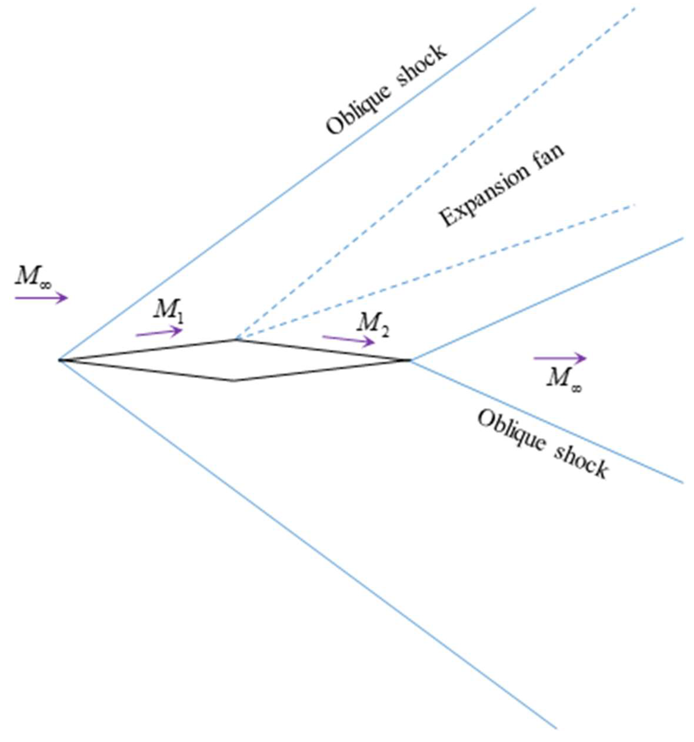
Figure 2.
Supersonic flow over a diamond airfoil with M∞ = 2 and AOA = 0. Mach contours (a) and Mach along the airfoil profile (b) for a numerical solution computed with the Tau solver. Analytic Mach values obtained with shock-expansion theory are shown as black dashed lines.
Figure 2.
Supersonic flow over a diamond airfoil with M∞ = 2 and AOA = 0. Mach contours (a) and Mach along the airfoil profile (b) for a numerical solution computed with the Tau solver. Analytic Mach values obtained with shock-expansion theory are shown as black dashed lines.
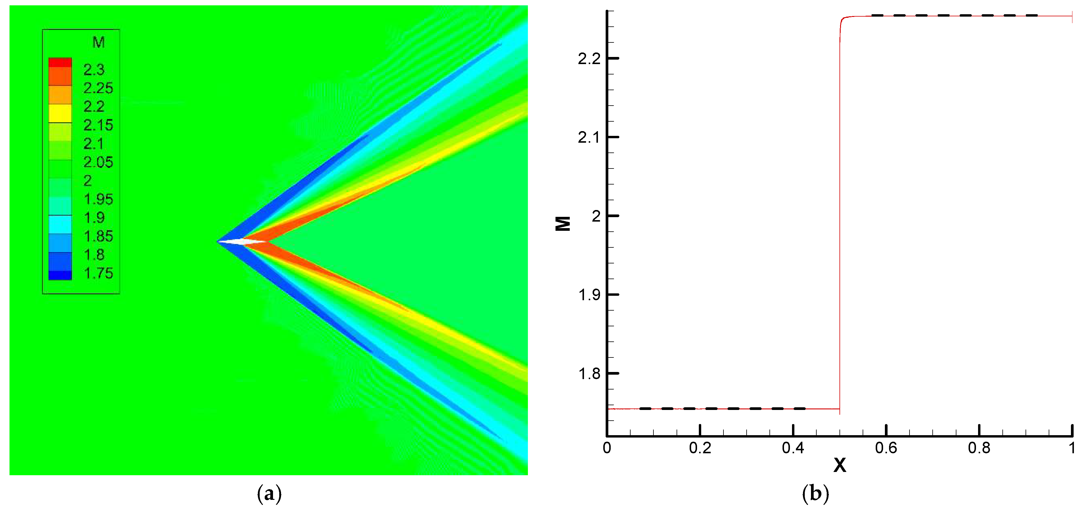
Figure 3.
Supersonic flow over a diamond airfoil with M∞ = 2 and AOA = 0. Contour plot of the drag adjoint density variable for a numerical solution computed with the Tau solver.
Figure 3.
Supersonic flow over a diamond airfoil with M∞ = 2 and AOA = 0. Contour plot of the drag adjoint density variable for a numerical solution computed with the Tau solver.
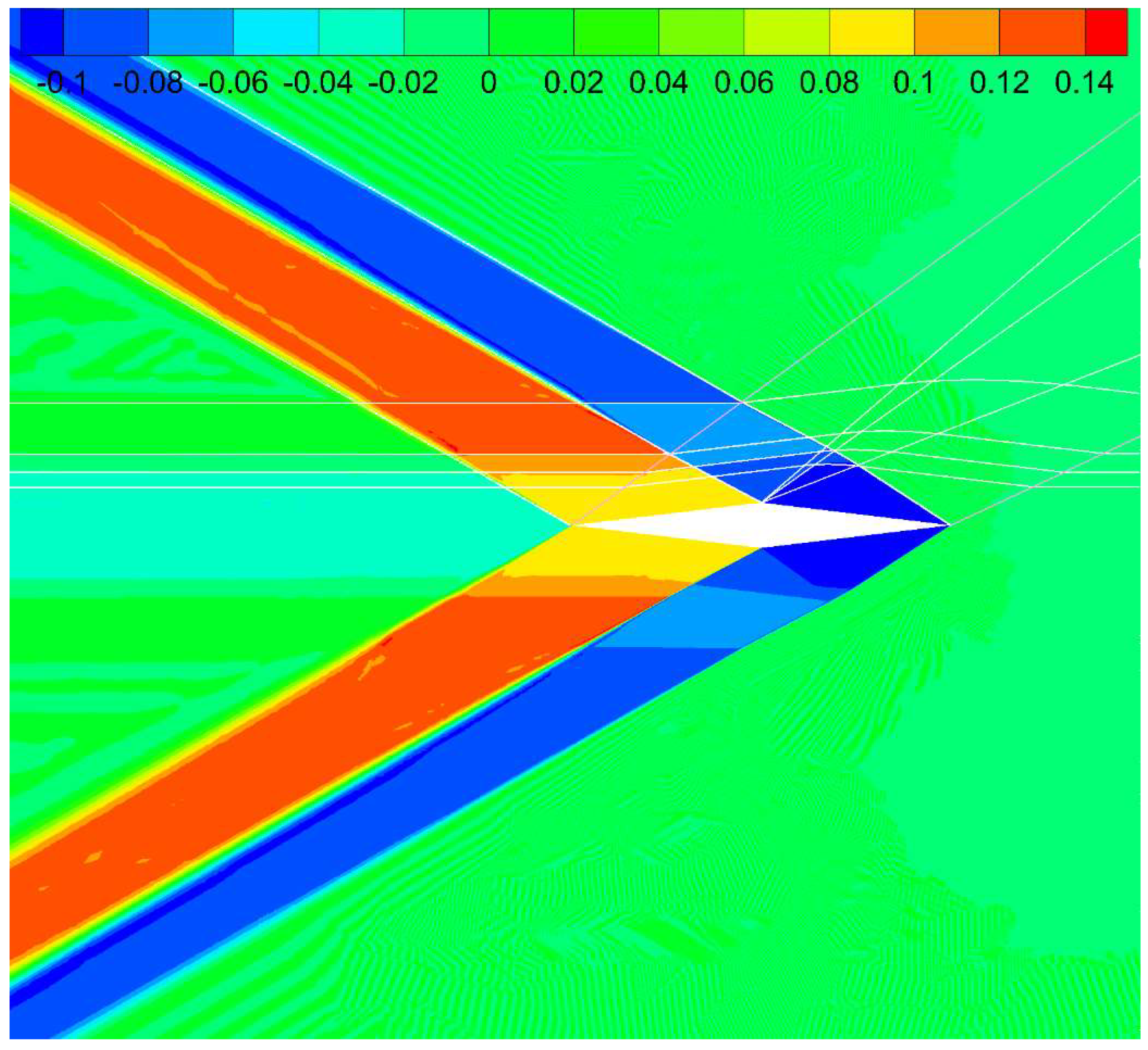
Figure 4.
Supersonic flow over a diamond airfoil with M∞ = 2 and AOA = 0. Adjoint variables along the wall for a numerical solution computed with the Tau solver. Analytic values as per eq. (37) and (55) are also shown as dashed red lines.
Figure 4.
Supersonic flow over a diamond airfoil with M∞ = 2 and AOA = 0. Adjoint variables along the wall for a numerical solution computed with the Tau solver. Analytic values as per eq. (37) and (55) are also shown as dashed red lines.
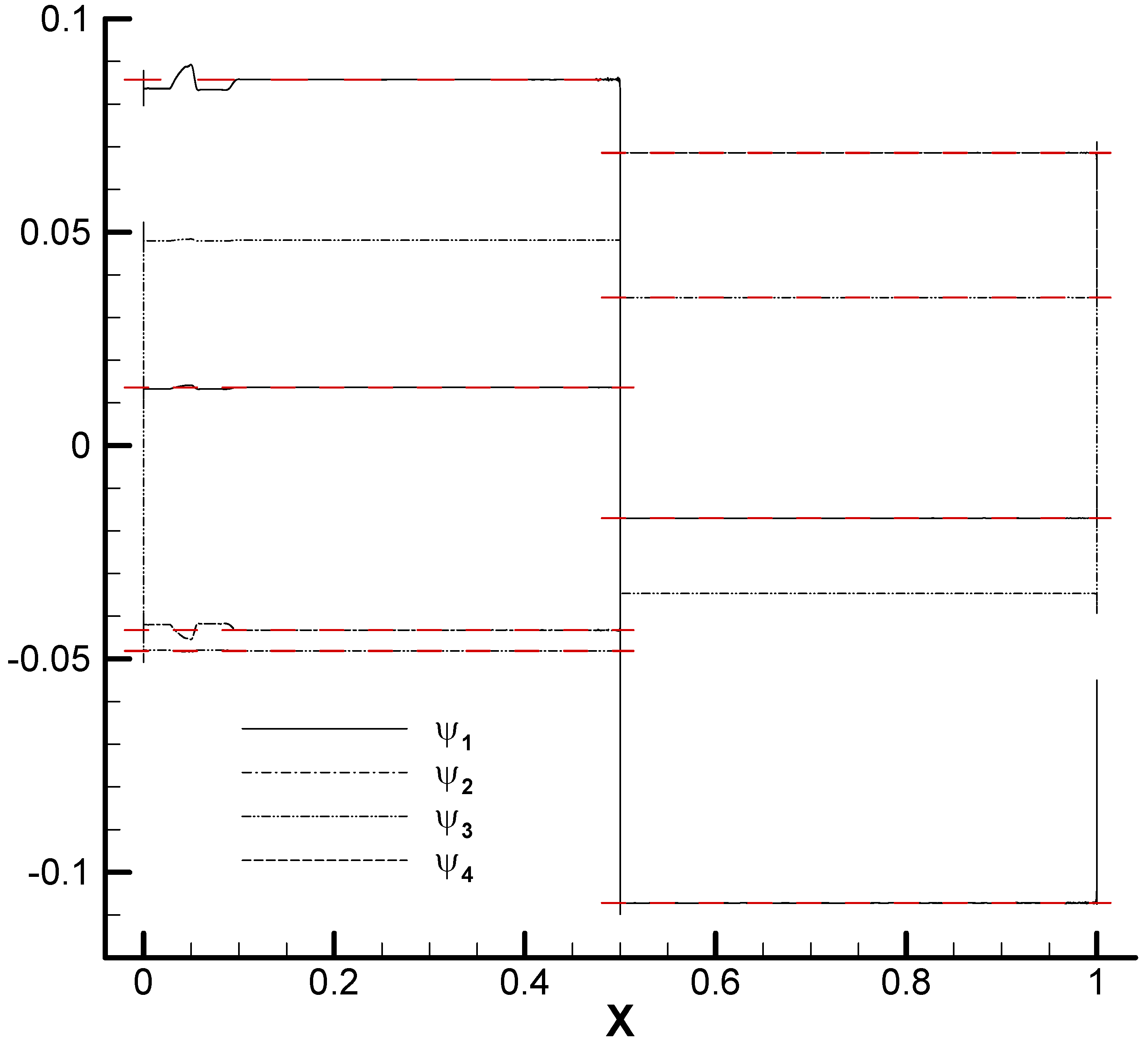
Figure 5.
Supersonic flow over a diamond airfoil with M∞ = 2 and AOA = 0. (a) First adjoint variable and Mach number along the (black) streamline indicated in panel (b) for a numerical solution computed with the Tau solver. The value of the adjoint variable along the airfoil profile is also shown for comparison.
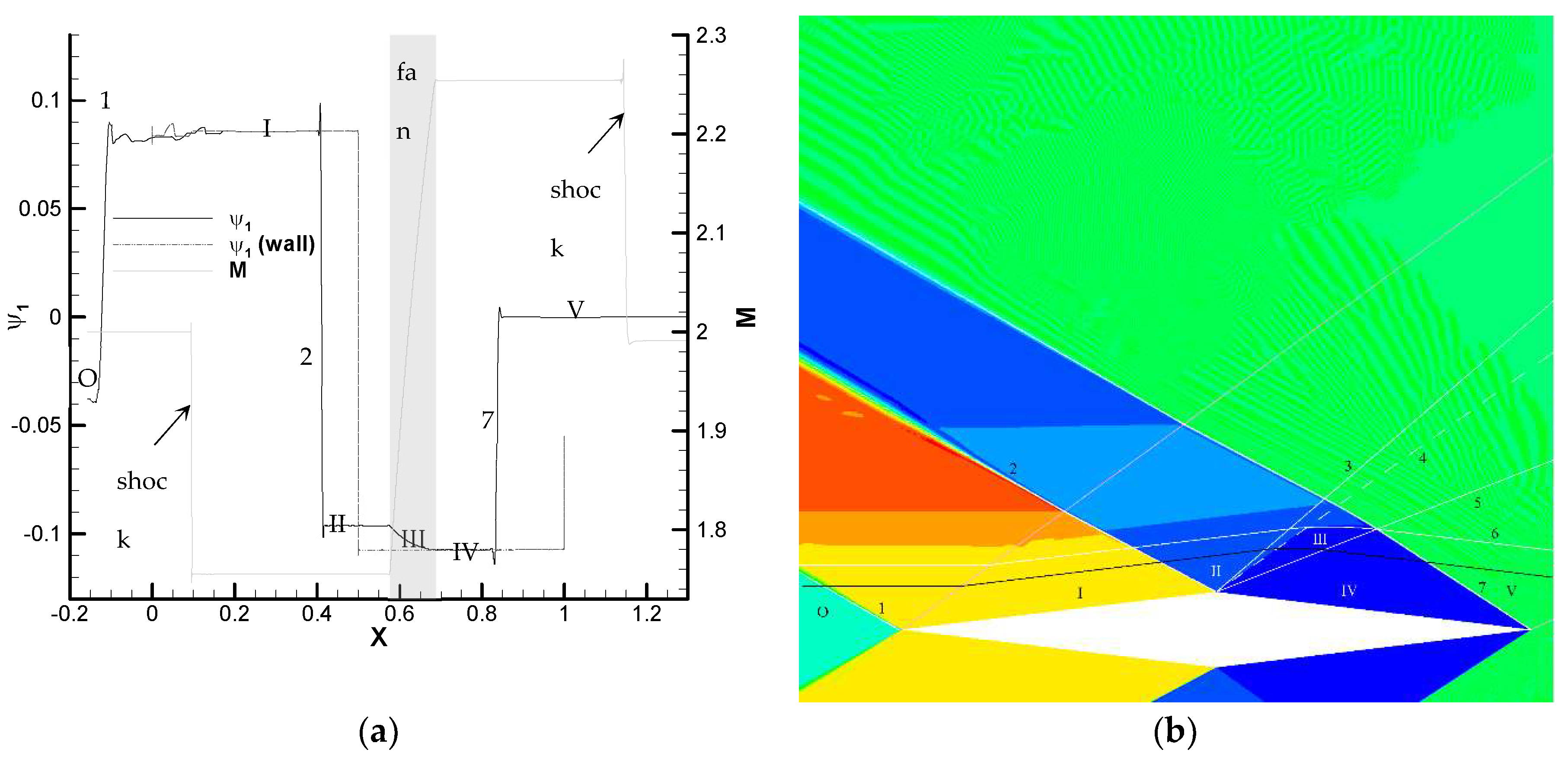
Figure 6.
Contour plot of the Riemann function associated with left-running characteristics C+ (with eigenvalue ) for a numerical solution computed with the Tau solver. This function is roughly conserved along left-running characteristics (upward diagonal) and continuous across right-running (downward diagonal) characteristics.
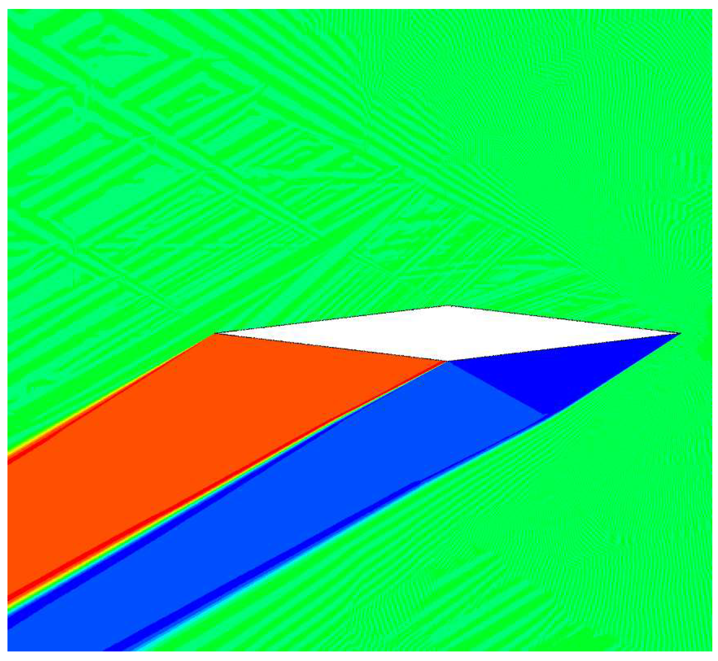
Figure 7.
Supersonic flow over a diamond airfoil with M∞ = 2 and AOA = 0. I2, I4 and Mach number along the streamline indicated in Figure 5 for a numerical solution computed with the Tau solver.
Figure 7.
Supersonic flow over a diamond airfoil with M∞ = 2 and AOA = 0. I2, I4 and Mach number along the streamline indicated in Figure 5 for a numerical solution computed with the Tau solver.
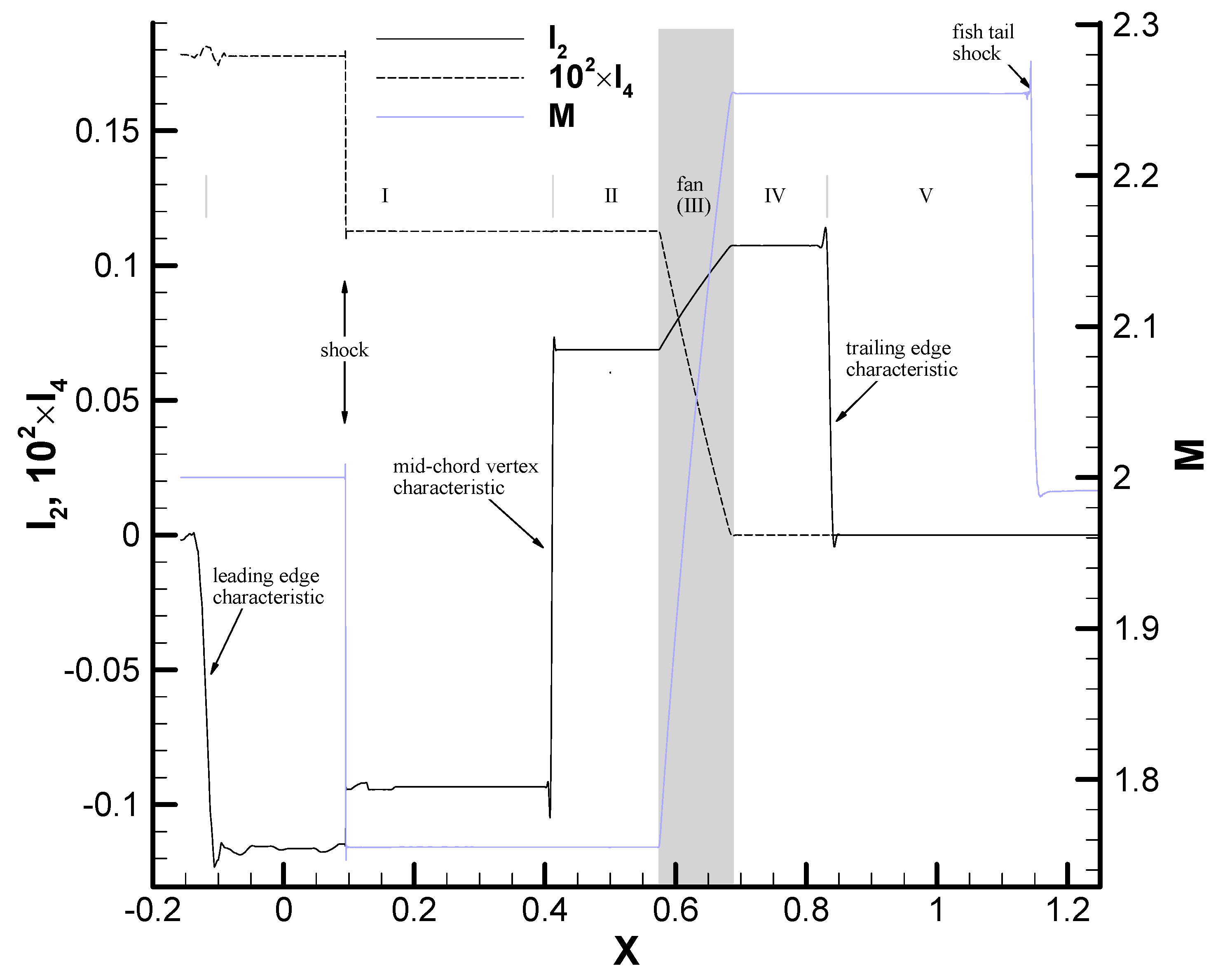
Figure 8.
Supersonic flow over a diamond airfoil with M∞ = 2 and AOA = 0. Adjoint variables and Mach number along the streamline indicated in Figure 5 for a numerical solution computed with the Tau solver. The analytic values for regions I, II and IV, as per eq. (37), (55) and (56), are shown as dashed red lines for comparison.
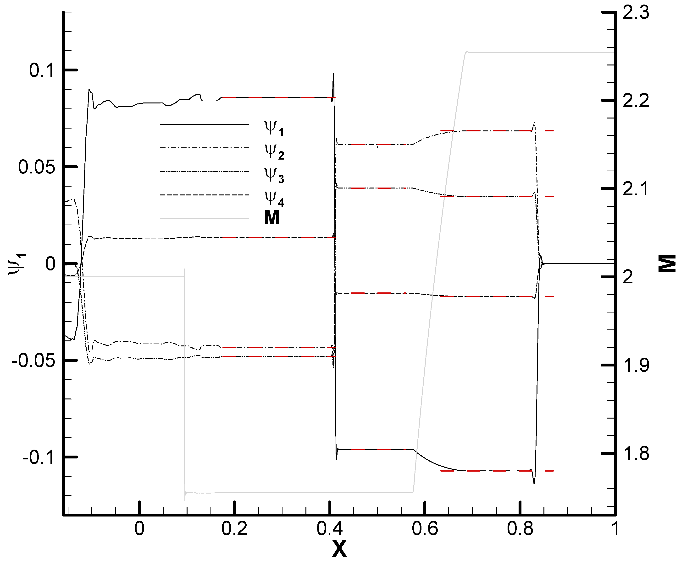
Figure 9.
Supersonic flow over a diamond airfoil with M∞ = 2 and AOA = 0. I2, I4 and Mach number (a) and adjoint solution (b) along Mach lines (3), (4) and (5) within the fan as indicated in Figure 5 for a numerical solution computed with the Tau solver. Analytic values are depicted as dashed red lines.
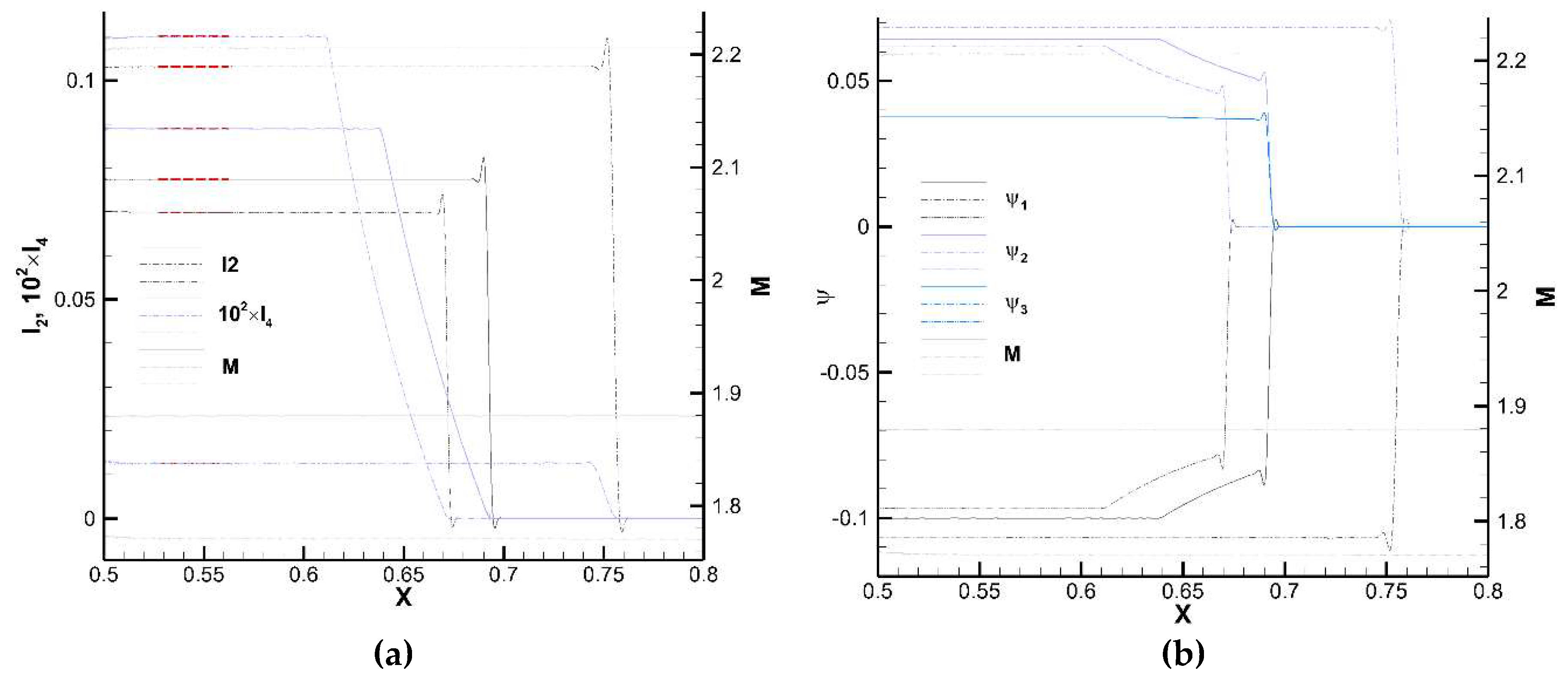
Figure 10.
Supersonic flow over a diamond airfoil with M∞ = 2 and AOA = 0. Sketch of the fan region.
Figure 10.
Supersonic flow over a diamond airfoil with M∞ = 2 and AOA = 0. Sketch of the fan region.
Disclaimer/Publisher’s Note: The statements, opinions and data contained in all publications are solely those of the individual author(s) and contributor(s) and not of MDPI and/or the editor(s). MDPI and/or the editor(s) disclaim responsibility for any injury to people or property resulting from any ideas, methods, instructions or products referred to in the content. |
© 2025 by the authors. Licensee MDPI, Basel, Switzerland. This article is an open access article distributed under the terms and conditions of the Creative Commons Attribution (CC BY) license (http://creativecommons.org/licenses/by/4.0/).
Copyright: This open access article is published under a Creative Commons CC BY 4.0 license, which permit the free download, distribution, and reuse, provided that the author and preprint are cited in any reuse.


