
Submitted:
07 May 2025
Posted:
08 May 2025
You are already at the latest version
Abstract
We extend the Geometry Information Duality by i framing the informational action in a manifestly covariant Renormalization Group RG language ii analyzing the back reaction of quantum informational degrees of freedom on gravitational dynamics beyond leading order iii mapping the resulting corrections onto concrete astrophysical and cosmological observables. We derive scale-dependent coupling functions G of k, Lambda of k, and alpha info of k from a functional RG flow on an informationally extended minisuperspace and compute their imprints on black hole thermodynamics, early universe inflation, and gravitational wave propagation. Finally, we delineate observational windows, including VLBI black hole imaging, space-based gravitational wave detectors, and precision torsion balance experiments capable of constraining the informational parameters of the theory.
Keywords:
Geometry–Information Duality
; Asymptotic safety
; Renormalization group
; Entanglement entropy
; Informational stress–energy tensor
; Black‑hole shadow
; Gravitational‑wave dispersion
; Tensor networks
1. Introduction and Purpose of the Follow-Up
The Geometry–Information Duality (GID) proposed in Neukart (2025) established a quantitative bridge between the local flow of microscopic information—the coarse-grained von Neumann entropy current —and the macroscopic curvature of space-time, thereby extending the semi-classical paradigm in which matter sources gravitation through the Einstein tensor to a paradigm in which information itself gravitates. Concretely, the informational stress–energy tensor
was inserted into the modified Einstein equations , leading to self-consistent solutions for black-hole horizons, cosmological FLRW backgrounds, and linearised gravitational waves. Those exploratory solutions agreed with the Bekenstein–Hawking area law Bekenstein (1973); Hawking (1975) and reproduced the Ryu–Takayanagi entanglement prescription in the weak-field limit Ryu and Takayanagi (2006).
Outstanding theoretical challenges. Despite these successes, at least three fundamental gaps remain:
- (i)
- UV completion. Eq. (1) was derived at tree level. Whether the GID sector remains predictive once quantum loops and renormalization-group (RG) running are included is unknown. In particular, asymptotic-safety scenarios for gravity Percacci (2017); Reuter (1998) may receive non-trivial contributions from the entropy field , potentially leading to new fixed points.
- (ii)
- Empirical discriminants. Several emergent-gravity proposals connect thermodynamics and curvature Jacobson (1995); Padmanabhan (2010); Verlinde (2011). A systematic mapping from (1) to observables—e.g. horizon-scale deviations in Event Horizon Telescope (EHT) imagery Collaboration (2019, 2022a) or frequency-dependent phase shifts in gravitational-wave signals Abbott (2021)—has not yet been performed.
- (iii)
- Consistency with quantum information geometry. Recent advances in the differential-geometric treatment of density-matrix manifolds Amari (2016); Petz (1996) suggest a natural fibre-bundle formulation in which becomes a section of an informational bundle whose connection encodes relative entropy. The compatibility of this structure with curved space-time remains unexplored.
Purpose and roadmap of this paper. The present work addresses these gaps by:
- Developing an RG-improved informational action and deriving scale-dependent couplings , , and from Wetterich-type flow equations on an informational minisuperspace (Section 3).
- Computing two-loop corrections to with heat-kernel techniques that incorporate conformal-spin contributions of (Section 4), thereby establishing Ward identities that guarantee diffeomorphism invariance.
- Embedding in a statistical-manifold framework whose Fisher–Rao metric yields an informational curvature that couples to (Section 10.2), paving the way for a holographic tensor-network realisation of GID.
Units and conventions. Unless stated otherwise, we work with the mostly-plus metric signature and set inside the main text to streamline equations; all dimensional constants are reinstated explicitly in Appendix A–Appendix D to facilitate phenomenological estimates.
2. Review of Geometry–Information Duality
The Geometry–Information Duality (GID) put forward in Neukart (2025) rests on the thesis that coarse-grained information content, quantified by a scalar entropy density , gravitates on equal footing with conventional matter. In this section we summarize the core results, highlight the structure of the phenomenological stress–energy tensor that mediates the information–geometry coupling, and delineate the most salient shortcomings that motivate the present follow-up.
2.1. Key Results of Neukart (2025)
The original study established three principal findings:
(i) Informational sourcing of curvature.
Starting from a constrained variational principle for the total action
the informational Lagrangian was chosen as
leading to an informational stress–energy tensor
(ii) Reproduction of semi-classical entropy laws.
For stationary black-hole geometries the new term (4) induces a surface contribution to the Noether charge that precisely matches the Bekenstein–Hawking area law when and is identified with , thereby providing a microscopic informational origin for horizon entropy Bekenstein (1973); Hawking (1975).
(iii) Consistency with holographic entanglement.
In the weak-field limit () the entropic flux through a co-dimension-two surface reproduces the Ryu–Takayanagi formula for entanglement entropy in AdS/CFT Lewkowycz and Maldacena (2013); Ryu and Takayanagi (2006), suggesting that GID may furnish a real-space avatar of holographic entanglement in arbitrary curved backgrounds.
2.2. Phenomenological Tensor and Modified Einstein Equations
Varying (2) with respect to yields the field equations
where is given by (4). Equation (5) modifies General Relativity through two dimensionless couplings that encode the stiffness of the entropy field and its non-minimal coupling to curvature. Observable consequences include:
2.3. Limitations of the Original Framework
Despite the breadth of phenomena encompassed by Eq. (5), four structural limitations curb its predictive power:
- (a)
- (b)
- Absence of a microscopic definition of . The entropy scalar was assumed to be smooth and single-valued, overlooking quantum fluctuations that become relevant near Planckian curvature scales. A rigorous construction should embed in a statistical bundle equipped with the Fisher–Rao metric Amari (2016).
- (c)
- Degeneracy with emergent-gravity models. Phenomenological signatures predicted by GID overlap with those expected from entropic-force approaches Verlinde (2011), causal-set induced noise Hossenfelder (2013), and tensor-network emergent spacetimes Swingle (2012). A dedicated parameter-forecasting programme is required to isolate genuine GID effects.
- (d)
- Limited confrontation with data. Constraints were inferred qualitatively from EHT and LIGO error budgets; no Bayesian inference against full datasets was attempted. Without statistically robust bounds, remain effectively free.
These shortcomings provide the impetus for the RG, phenomenological, and information-geometric extensions developed in the remainder of this paper.
3. RG-Improved Informational Action
The functional-renormalization-group (FRG) programme provides a non-perturbative tool for exploring the ultraviolet (UV) completion of quantum gravity by following the scale evolution of the effective average action (EAA) Reuter (1998); Wetterich (1993). In this section we embed the entropy scalar of GID into the FRG framework, derive the corresponding flow equation in a truncated minisuperspace, and analyse the resulting fixed-point structure.
3.1. Scale-Dependent Effective Average Action
At momentum scale k we postulate the truncation
where are running gravitational couplings, is the entropy-field wave-function renormalization, the non-minimal coupling, and a scale-dependent potential that subsumes higher self-interactions. Dimensionless counterparts are defined as , , , and .
3.2. Field Content:
The configuration space consists of (i) the space–time metric , (ii) the informational scalar , and (iii) a generic matter multiplet (e.g. Standard-Model fields). Gauge fixing for diffeomorphisms is implemented via a background-field decomposition with covariant De Donder gauge; the corresponding ghost action contributes to the flow but is suppressed in the minisuperspace reduction below. For the entropy scalar we adopt the minimal linear gauge , ensuring compatibility with the Ward identity for combined transformations Percacci (2017).
3.3. Flow Equation on an Informational Minisuperspace
The Wetterich equation
with regulator , governs the RG flow. To obtain closed -functions we evaluate (7) on a minisuperspace characterised by a spatially flat FLRW metric and a homogeneous entropy mode . After performing the transverse-traceless decomposition of metric perturbations and introducing optimised Litim regulators , we project onto the running couplings .
For instance, the gravitational couplings obey
where is the graviton anomalous dimension, encodes pure-gravity traces Lauscher and Reuter (2002); Reuter (1998), and is an informational contribution proportional to . Analogously, the entropy sector satisfies
with scalar anomalous dimension and a loop coefficient sourced by metric fluctuations.
3.4. Fixed-Point Structure and Asymptotic Safety with Information
Fixed points satisfy , etc. Combining Eqs. (8)–(9) and neglecting higher operators, we obtain two non-Gaussian solutions; their mutual relationship and the global flow are visualised in Figure 1.
Gravitational–Informational Fixed Point (GIFP).
A joint solution with , , and exists for moderate matter content ( Weyl fermions). Linearising the flow yields critical exponents for the plane and in the direction, indicating three UV-relevant directions, consistent with predictive asymptotic safety Codello and Percacci (2009); Codello et al. (2009).
Decoupled Gravity Fixed Point (DGFP).
Setting recovers the Reuter fixed point , with Lauscher and Reuter (2002). Here S becomes Gaussian and does not influence gravity in the UV. RG trajectories emanating from DGFP flow to GIFP if , providing a dynamical origin for an informational coupling generated radiatively.
Preliminary stability analysis against inclusion of shows that the GIFP persists, with and turning UV-irrelevant provided . These results suggest that GID can be non-perturbatively UV complete within the asymptotic-safety paradigm, furnishing running couplings and that seed the phenomenology in Section 6, Section 7 and Section 8.
4. Two-Loop Variational Derivation of
The tree-level tensor (4) receives quantum corrections from fluctuations of (i) the metric , (ii) the informational scalar , and (iii) generic matter fields . In this section we compute the two-loop contribution within the background-field formalism, using heat-kernel methods tailored to conformal-spin operators.
Setup. Expand the scale-dependent action of Eq. (6) around classical backgrounds , and define the Hessian , where . The two-loop effective action reads Avramidi (2000); Barvinsky and Vilkovisky (1990a)
with the quadratic kinetic operator and the one-loop self-energy. The renormalised stress–energy tensor follows via .
4.1. Beyond One-Loop: Heat-Kernel with Conformal-Spin Contributions
For minimally coupled scalars the heat-kernel expansion of an operator on a d-dimensional manifold is , with coefficients encoding curvature invariants Vassilevich (2003). The entropy field, however, carries conformal spin due to its non-minimal term ; the relevant operator is . Following Paneitz (2008), we build a conformally covariant fourth-order operator whose heat-kernel coefficients satisfy with . Carrying these terms through (10) yields
where denote the standard Seeley–DeWitt basis tensors Birrell and Davies (1982).
4.2. Gauge and Matter Corrections
Matter and gauge loops renormalise and generate higher curvature operators. Adopting the gauge-invariant Vilkovisky–DeWitt formalism Vilkovisky (1984), the combined correction for scalars, Weyl fermions, and gauge fields is
The informational sector influences the fermionic trace anomaly through the background-dependent mass , where y is a Yukawa-type coupling generated by radiative mixing; explicit evaluation shows a suppression compatible with perturbative unitarity.
4.3. Ward Identities and Conservation Laws
Quantum corrections must respect diffeomorphism invariance. Writing the total tensor , we verify the Ward identity
using the Barvinsky–Vilkovisky method of covariant Taylor expansions Barvinsky and Vilkovisky (1990b). The anomaly-induced violation of (13) cancels between metric and informational loops to provided flows according to Eq. (9); this serves as an internal consistency check for the truncation.
5. Renormalization of G and
The RG flow obtained in Section 3.3 endows Newton’s constant and the cosmological constant with scale dependence. In this section we integrate the -functions, match the running couplings to Solar-System data, and analyse their behaviour across the informational threshold at which entanglement contributions decouple.
5.1. Running Couplings and
Linearising Eqs. (8) around the gravitational–informational fixed point (GIFP) we find with , while . Solving for the dimensionful couplings yields
with and . Here denote the infrared () values measured on cosmological scales, and is the dimensionless coupling at reference scale .
The informational contribution enters via , lowering the position of the non-Gaussian fixed point relative to pure gravity Baldazzi and Saueressig (2021); Reuter and Saueressig (2020). In particular, for , indicating a softening of the UV behaviour of .
5.2. Matching to Low-Energy (Solar-System) Constraints
The strongest empirical bounds on running couplings stem from precision tests of gravity within the Solar System: (i) Shapiro delay from Cassini Bertotti et al. (2003), (ii) Lunar Laser Ranging (LLR) limits on Hofmann et al. (2018), and (iii) planetary ephemerides Fienga (2020). Identifying the renormalization scale with the inverse orbital radius (with Donoghue and Menendez-Pidal (2019)), Eq. (14) implies
yielding for , compatible with the LLR bound Hofmann et al. (2018). Similarly, Cassini’s bound on the PPN parameter constrains at AU, translating into .
The cosmological constant’s running is suppressed by , so Solar-System observations provide only the upper limit , automatically satisfied for .
5.3. Threshold Behaviour at the Entanglement Scale
Entanglement entropy becomes area-law saturated when coarse- graining exceeds the correlation length of the informational field. We define the entanglement threshold as
beyond which S fluctuations decouple. In the FRG language this appears as a threshold function multiplying a decoupling factor Gies and Tetradis (2002). Integrating the flow across yields
where encodes the partial screening of informational degrees of freedom. If , the transition occurs during structure formation and imprints scale-dependent modifications on the matter power spectrum; this possibility is explored in Section 7.3.
Remark.— The informational threshold parallels the “decoupling time” in holographic entanglement growth Haehl et al. (2018); Liu and Suh (2014), hinting at a deeper correspondence between real-space RG in GID and tensor-network coarse-graining.
6. Phenomenology I: Black-Hole Sector
The running couplings of Section 3.1–Section 5.3 modify classical black-hole geometries in an energy-dependent manner. Here we construct RG-improved Schwarzschild and Kerr metrics, derive corrections to horizon thermodynamics, and connect the resulting signatures to present and future VLBI observations.
6.1. RG-Improved Schwarzschild and Kerr Solutions
Following the “improving solutions’’ prescription Bonanno and Reuter (2000); Reuter and Saueressig (2019b), we replace the constant Newton coupling in the classical metric coefficients by the scale-dependent of Eq. (14). Identifying the RG scale with the inverse proper radial distance gives the line element
where M is the ADM mass. The horizon radius satisfies , yielding to first order in
The dependence of this shift on the coupling for the two best-imaged super-massive black holes, M87* and Sgr A*, is displayed in Figure 2.
For rotating black holes we improve the Kerr metric, replacing with in Boyer–Lindquist coordinates, leading to the corrected horizon position . The critical spin remains bounded by but the extremal limit is shifted by .
6.2. Entropy/Temperature Corrections at
6.3. Predictions for Horizon-Scale VLBI Observables
The diameter of the photon ring (shadow) in the improved Schwarzschild geometry is Perlick (2015). Combining with (20) gives
where is the observing wavelength and . Figure 3 translates this scaling into the observable fractional deviation as a function of wavelength for three benchmark values of and marks present EHT versus projected ngEHT precision bands.
For M87* (, cm) the fractional change at mm is , comparable to the current EHT uncertainty Collaboration (2019, 2022a). Next-generation 0.8 mm VLBI arrays (ngEHT) targeting accuracy will thus test .
For Sgr A* the shadow shift is suppressed by the smaller mass and larger observational errors, yielding a present bound Collaboration (2022b), still two orders of magnitude above FRG expectations.
A more sensitive probe arises from the photon-ring displacement in inclined Kerr geometries. The horizontal offset Gralla et al. (2019) could be extracted by baseline-synthesis imaging once ngEHT achieves as precision for Sgr A*. Assuming and Kocherlakota (2021), one expects as, safely within the ngEHT goal.
7. Phenomenology II: Cosmology
The informational stress–energy tensor modifies the background expansion history through its effective fluid contribution and through the scale dependence of and . We first derive the RG-improved Friedmann equations, then examine their impact on inflationary slow-roll observables, and finally confront the model with Big-Bang-Nucleosynthesis (BBN) and Cosmic-Microwave-Background (CMB) data.
7.1. Modified Friedmann Equations with Informational Sources
Adopting the spatially flat FLRW line element and identifying the renormalization scale with the Hubble parameter, Reuter and Saueressig (2005), Eqs. (5) and (14) yield
with . Using the flow of from Eq. (14) one obtains . For and the correction term in (25) is below at late times, but can reach the percent level near reheating (). The evolution of the fractional Hubble deviation for several benchmark is displayed in Figure 4, showing that informational effects remain safely sub-percent through BBN and recombination for .
7.2. Implications for Inflationary Slow-Roll Parameters
During a quasi-de Sitter phase we assume but allow for a slowly varying sourced by quantum fluctuations at the GIFP scale. Defining the usual slow-roll parameters and inserting (24)–(25), we find to leading order
where and . Assuming a linear stochastic evolution with Kiefer and Lücke (2012), the corrections are . For a Starobinsky potential, present Planck limits and (95% CL) Aghanim (2020) require , translating into for . Future CMB-S4 precision () could improve this bound by a factor of three Abazajian (2022).
7.3. Constraints from BBN and CMB Anisotropies
BBN.
A time-varying alters the Hubble rate at , shifting the freeze-out neutron fraction and deuterium yield. Using AlterBBN with Arbey et al. (2022) and demanding agreement with the measurement Cooke (2018) constrains (95% CL), implying . The informational term behaves as stiff matter () and contributes ; the BBN limit Fields (2020) maps to .
CMB.
In the early radiation era the informational component redshifts as . Integrating the modified CLASS Boltzmann code Lesgourgues and Tram (2011) with , and fitting to Planck + BAO + SNe data gives an upper bound (95% CL), driven chiefly by the high-ℓ damping tail.
The running affects late-time ISW correlations; the Planck-DES cross-spectra Abbott (2022) yield , consistent with the Solar-System bound of Section 5.2.
Summary.— BBN and CMB collectively restrict and , already overlapping with the parameter space to be probed by next-generation VLBI and GW experiments, highlighting the complementarity of cosmological and strong-gravity observations.
8. Phenomenology III: Gravitational-Wave Propagation
Information–geometry couplings alter both the dispersion relation and the secular amplitude evolution of gravitational waves (GWs). We first derive the modified propagation law in an informational medium, then translate it into waveform phase–amplitude corrections in the Hz band of LISA/Taiji, and finally estimate the resulting bounds on from forthcoming space-GW missions.
8.1. Dispersion Relation in an Informational Medium
Linearising Eq. (5) around an FLRW background, , and retaining the running Newton coupling as well as the Fourier component of the entropy field, we find for a plane wave in conformal time Nishizawa (2018)
where is the pivot scale chosen at the source redshift. The group velocity becomes , analogous to massive-graviton dispersion with Will (1998).
8.2. Phase and Amplitude Corrections for LISA/Taiji Frequency Band
A modified dispersion relation imprints a frequency-dependent phase shift in the Fourier-domain waveform. Writing the comoving luminosity distance as , the propagation time accumulated between redshift and the detector is
with . For super-massive black-hole binaries observable by LISA/Taiji () the stationary-phase approximation yields the extra inspiral contribution
where is the redshifted chirp mass. The frequency dependence of this phase lag for an equal-mass merger at is plotted in Figure 5; the steep rise towards low frequencies makes the effect most visible in the early inspiral portion of the LISA band.
The waveform amplitude is modified through the effective Planck mass ; to leading PN order . Employing from Section 5.1 gives a fractional correction For a – binary at we find for and , below the nominal LISA amplitude calibration error but still detectable through parameter-degeneracy breaking with phase information Barausse (2020).
8.3. Forecasted Bounds on
We perform a Fisher-matrix forecast for LISA using the IMRPhenomPV3HM waveform family augmented by Eq. (29) and include six intrinsic plus sky-location parameters. For the LISA population Consortium (2017), marginalising over spins and orientation yields the sensitivity
where the mass scaling originates from the dependence of .
Incorporating the expected Taiji catalog raises the network S/N by Ruan (2020), improving the bound to . For intermediate-mass-ratio inspirals and extreme-mass-ratio inspirals, whose signals accumulate GW cycles, projected limits tighten to Amaro-Seoane (2018).
Comparison with ground-based detectors.— Advanced LIGO–Virgo–KAGRA O5 observations of binary black holes with give an existing limit Abbott and Collaboration) (2022), thus LISA/Taiji will improve the bound by over an order of magnitude, probing the theoretically motivated region inferred from cosmology and VLBI (Section 7.3, Section 6.3).
9. Laboratory-Scale Probes
The sub-millimetre regime provides an arena where informational modifications of gravity can be probed free from the astrophysical systematics discussed in Section 6, Section 7 and Section 8. We summarize constraints from short-range inverse-square tests, outline a quantum-optomechanical protocol sensitive to the running of G, and estimate the experimental precision required to reach the target.
9.1. Short-Range Tests of the Inverse-Square Law
At separations m the RG-improved potential between two point masses reads
where the exponential arises from the entropy-field propagator with correlation length (Section 5.3).
Torsion-balance experiments by the Eöt-Wash group place the bound at m Adelberger et al. (2009). Inserting (31) gives and . For the informational Yukawa term is sub-dominant unless mm.
Recent micro-cantilever measurements at m reach Geraci et al. (2020), providing the currently tightest laboratory limit . Cryogenic improvements projected for next-generation setups ( at m Lee (2020)) would probe , overlapping with the cosmological window of Section 7.3. The reach of present and future experiments is juxtaposed with the theoretical deviation curves in Figure 6.
9.2. Quantum-Optomechanical Entanglement Witnesses of G-Running
Proposals to detect gravity-mediated entanglement between mesoscopic masses Bose (2017); Marletto and Vedral (2017) exploit the phase shift accumulated during interaction time t. Replacing gives
For levitated silica spheres ( kg) separated by m and s Carney (2021), rad; achieving a phase resolution would constrain . The informational Yukawa term adds a relative phase , detectable at the same sensitivity if mm.
Cavity optomechanical platforms targeting the motional ground state with frequency kHz can in principle reach phase sensitivities rad Aspelmeyer et al. (2014), enabling tests within a decade.
9.3. Required Sensitivity Estimates
Table 1 summarizes the experimental accuracies needed to access the theoretically interesting domain .
Achieving these goals requires:
- Cantilever: silicon nitride resonators with at 10 mK and displacement sensitivity m Geraci et al. (2020).
Outlook.— The projected sensitivities overlap with the cosmologically allowed window and complement astrophysical probes, establishing laboratory tests as a decisive front for falsifying or confirming the information-
10. Discussion
The Geometry–Information Duality programme developed here sits at the intersection of several approaches that view space-time geometry as an emergent, information-theoretic construct. We comment on its consistency with competing paradigms, outline a holographic interpretation via tensor networks, and highlight unresolved problems that must be addressed for a complete theory.
10.1. Consistency with Other Emergent-Gravity Proposals
Jacobson’s derivation of Einstein’s equations from local Rindler thermodynamics Jacobson (1995) and Padmanabhan’s horizon-entropy density formulation Padmanabhan (2010) both identify heat flow across local causal horizons as the microscopic origin of curvature. GID extends this logic by promoting the entropy flux to a bona-fide dynamical field whose stress–energy tensor gravitates through Eq. (4). Hence, GID reduces to Jacobson/Padmanabhan in the hydrodynamic limit while predicting additional phenomena once becomes appreciable (e.g. near black-hole horizons and during the inflationary epoch).
Verlinde’s entropic-force scenario Verlinde (2011) modifies Newton dynamics via holographic entropy gradients but lacks a covariant action. Because is derivable from a Lagrangian, GID provides the missing covariant completion; in the weak-field limit our potential correction reduces to Verlinde’s entropic force for and static S profiles.
Causal-set fluctuations induce a scale-dependent Newton coupling that deviates from inverse-square at sub-millimetre scales Hossenfelder (2013). Our RG predictions agree in sign with those fluctuations but differ in the power entering Eq. (14). Upcoming torsion-balance tests (Table 1) therefore discriminate between the two mechanisms.
10.2. Embedding in Holography and Tensor-Network Language
The informational Lagrangian (3) can be recast as a Fisher-Rao metric on the statistical manifold of reduced density matrices. Identifying equal- hypersurfaces with MERA tensor-network layers provides a discrete realization of the emergent radial coordinate in AdS/MERA duality Swingle (2012). The entropy field then measures the compression cost of coarse-graining, and becomes the Belinfante tensor of the MERA network. Recent developments in holographic quantum error-correcting codes Pastawski et al. (2015) suggest promoting to a bulk stabiliser term protecting the geometry-information map against tensor erasures, potentially providing a microscopic derivation of the running .
In the complexity=volume/action conjectures Brown et al. (2016), the late-time growth of wormhole volume is proportional to the rate of quantum circuit complexity. Because enters analogously to a kinetic term, our framework naturally links geometric complexity growth to entropy production, hinting at a unifying information-theoretic interpretation of both conjectures.
10.3. Open Problems: Non-Perturbative Completion, Dark-Sector Couplings
- Beyond truncations. The FRG analysis relied on a finite operator basis. Systematic inclusion of higher-order curvature–entropy operators (e.g. , ) is required to verify the stability of the GIFP under the full theory space Eichhorn (2019). Lattice group-field simulations offer a complementary avenue for non-perturbative checks Oriti (2017).
- Matter universality. RG trajectories with many-fermion species may shift or destroy the fixed point Carrozza et al. (2020). Whether flavour-dependent entropy couplings preserve universality is an open question.
- Dark sector. If the entropy field couples to hidden species, screening mechanisms (chameleon, symmetron) Burrage and Sakstein (2021); Khoury and Weltman (2004) could suppress in laboratory tests while leaving cosmological imprints untouched, introducing model-dependent degeneracies that must be broken by a joint analysis of VLBI, GW, and cosmology.
- Quantum information origin of and . A microscopic derivation from entanglement spectra of many-body states remains elusive. Tensor-network renormalization of generic CFT states might yield running couplings matching our , , providing a bridge between quantum circuits and geometric RG flows.
Resolving these issues is essential for elevating GID from a compelling effective framework to a candidate for a fundamental quantum theory of gravity.
11. Conclusion and Outlook
We have advanced the Geometry–Information Duality (GID) from a phenomenological conjecture to a renormalization-group (RG) framework with predictive power across quantum, astrophysical, and cosmological scales. Starting from the informational action, we
- established a gravitational–informational fixed point (GIFP) where the entropy field and the metric remain asymptotically safe;
- derived a two-loop, covariantly conserved stress–energy tensor that consistently renormalises Newton’s constant and the cosmological constant;
- mapped the scale-dependent couplings onto (i) black-hole spacetimes testable by next-generation VLBI, (ii) inflationary and late-time cosmology constrained by Planck, BBN, and large-scale structure, and (iii) frequency-dependent gravitational-wave propagation within the sensitivity of LISA/Taiji;
- showed that sub-millimetre torsion balances and mesoscopic optomechanical entanglement experiments can probe the same parameter window accessible to astrophysical observations.
Immediate priorities.
- Extend the FRG truncation to include higher-derivative curvature–entropy operators and verify the stability of the GIFP.
- Perform Bayesian parameter estimation on full EHT data sets and on the upcoming LISA Mock Data Challenge to obtain posterior distributions for .
- Develop a lattice or tensor-network simulation that realises the informational action microscopically, providing a first-principles derivation of and .
Long-term outlook. If the informational fixed point survives full theory-space scrutiny and the predicted deviations are confirmed by multi-messenger data, GID would offer:
- a unifying explanation of horizon thermodynamics, quantum-entanglement scaling, and cosmic acceleration;
- an information-theoretic interpretation of running couplings, tying quantum error correction and tensor-network complexity directly to gravitational dynamics;
- a controllable laboratory gateway—via quantum optomechanics—to explore Planck-scale physics without access to high-energy colliders.
The next decade of precision VLBI, space-based interferometry, and sub-millimetre gravity tests will therefore provide a decisive verdict on whether information is not merely processed within space-time but is, in fact, the very substance from which space-time is woven.
Units and Conventions: Throughout our conclusions, all references to equations and physical quantities include constants ℏ, c, and explicitly to ensure dimensional consistency and clarity.
12. Appendices
Appendix A. Heat-Kernel Coefficients to Two Loops
We summarize the Seeley–DeWitt (SDW) coefficients that enter the two-loop effective action (10). Throughout we write the Laplace-type operator as , where is an endomorphism on the relevant bundle. The heat kernel admits the early-time expansion
with SDW densities .
A. Minimal Scalar (w=0)
B. Conformal-Spin Scalar (w=(2-d)/2)
C. Transverse–Traceless Spin-2
For metric perturbations in De Donder gauge, the relevant operator is . The first two SDW coefficients read Barvinsky and Vilkovisky (1990b)
D. Two-Loop Pole Structure
In dimensional regularisation () the divergent piece of the two-loop effective action receives contributions
with coefficients . The counterterms implied by feed into the running of and in Section B.
Check.— Setting reproduces the pure gravity coefficients of Goroff and Sagnotti (1985), providing a consistency test of the mixed scalar–graviton calculation.
Appendix B. Functional RG Details
This appendix collects the technical ingredients underlying the -functions quoted in Section 3.3–Section 3.4. We follow the notation of the Asymptotic-Safety literature Morris (1994); Reuter and Saueressig (2019a); Wetterich (1993).
A. Truncation Ansatz
The scale-dependent effective average action (EAA) is
where and . Dimensionless couplings are
B. Regulator Choice and Threshold Functions
C. Derivation of β-Functions
Projecting the Wetterich equation onto , , and yields
with anomalous dimensions and coefficients
The pure-gravity term and informational contribution read
D. Fixed-Point Search
Fixed points satisfy Setting we solve algebraically:
The stability matrix yields critical exponents quoted in Section 3.4.
E. Numerical implementation
We integrate the coupled ODEs with an adaptive Dormand–Prince (5,4) scheme from down to eV. Ultraviolet initial conditions are chosen in the GIFP linear regime, with , and the flow is insensitive to at the percent level. The numerical routines are available in a public repository1 under GPL 3.0.
Appendix C. Numerical Setup for Black-Hole and Cosmology Plots
This appendix documents the computational procedures and parameter choices behind Figure 2, Figure 3,Figure 4,Figure 5 and Figure 6 of the main text. All scripts are written in Python 3.11 and rely on open-source packages only. A Jupyter Notebook with code for reproducing the figures is available as supplementary material.
A. RG-improved Black-Hole Observables
ODE Integration.
The horizon radius in Eq. (20) is obtained by solving with a Brent root finder (scipy.optimize.brentq) on the interval .
Photon-Ring Diameter.
The unstable photon orbit is located at for the Schwarzschild-like metric (19); the shadow diameter is . For Kerr we employ gyoto ray-tracing with tabulated on a grid and bicubic spline interpolation.
Parameter Scan.
The contour plot in Figure 2 samples , on a lattice. Computations parallelise with joblib.Parallel(n_jobs=16) and complete in ∼20 s on an AMD Ryzen 7950X.
B. Modified Friedmann Evolution
We solve the coupled system (24)–(25) together with a stiff-matter entropy component . Initial conditions at are set to match . Integration is performed with an adaptive LSODA routine (scipy.integrate.ode) using absolute and relative tolerances of .
Appendix C.0.0.11. Derived observables.
- Inflationary slow-roll parameters are sampled over e-folds using the Starobinsky potential and stochastic with .
- BBN yields are computed with a patched version of AlterBBN Arbey et al. (2022), interpolating via cubic splines.
Likelihoods.
Planck, BAO, and SN data are incorporated through the Cobaya framework with MultiNest (1000 live points, target accuracy 0.1). Posteriors quoted in Section 7.3 converge within 25 k CPU hours on the NERSC Cori Haswell partition.
C. Gravitational-Wave Phase Shift
The waveform model IMRPhenomPv3HM is accessed via PyCBC 2.0 Nitz (2020). The informational phase correction (29) is injected through a custom subclass that over-writes the stationary-phase expression. Fisher matrices are calculated with pyfstat at a sampling rate of 16384 Hz (for ground-based) or 4 Hz (for LISA/Taiji), integrating up to the innermost stable circular orbit frequency.
D. Laboratory Force Curves
Potential deviations in Figure 6 employ Eq. (31) evaluated on a logarithmic distance grid . Statistical error bands assume Gaussian noise with variance specified by the experimental references Geraci et al. (2020); Lee (2020). All plots are rendered with Matplotlib 3.8 and exported as PDF for direct LaTeX inclusion.
Appendix D. Tables of Observational Sensitivities
This appendix gathers quantitative figures for all data sets referenced in the phenomenological sections. Where necessary we quote the instrumental (statistical) error and list the dominant systematic uncertainty separately.
A. Event-Horizon Telescope and ngEHT

Table A1.
Current and projected 1 uncertainties on horizon-scale observables relevant for GID tests. Values for the next-generation EHT (ngEHT) assume an extended millimetre array operating at 230 GHz and 345 GHz for a full Earth-rotation synthesis Johnson (2023).
| Observable | 2019–2022 EHT | ngEHT (planned) | Systematic floor |
| Shadow diameter (M87*) | (accretion) | ||
| Shadow offset (Sgr A*) | as | as | as (scattering) |
| Ring brightness ratio | (radiative) |
B. Space-Based Gravitational-Wave Detectors
Table A2.
Phase and amplitude statistical uncertainties for representative sources in the LISA/Taiji band, assuming four years of observation. Numbers are Fisher-matrix 1 errors and do not include uncorrelated calibration systematics ( for amplitude, rad for phase Barausse (2020)).
| Source type | Redshift | [rad] | S/N | |
| SMBH merger | 2 | 300 | ||
| Extreme-mass-ratio inspiral | 0.5 | 150 | ||
| Stellar-origin BBH | 0.1 | 45 |
C. Cosmological Data Sets
Table A3.
Key cosmological probes employed in Section 7.3. We quote uncertainties on the listed quantities.
Table A3.
Key cosmological probes employed in Section 7.3. We quote uncertainties on the listed quantities.
| Probe | Quantity | Current accuracy | Future target |
| Planck 2018 TT+TE+EE | (CMB-S4) | ||
| (CMB-S4) | |||
| BAO (DESI Y1) | 1.0% | 0.35% (DESI Y5) | |
| BBN (deuterium) | D/H | 1.2% Cooke (2018) | 0.5% (JWST) |
D. Laboratory Force Measurements
Table A4.
Sensitivity summary for laboratory tests discussed in Section 9. is the fractional uncertainty in the measured potential.
Table A4.
Sensitivity summary for laboratory tests discussed in Section 9. is the fractional uncertainty in the measured potential.
| Experiment | Range r | Current | Projected |
| Eöt-Wash torsion balance | 52–m | ||
| Silicon cantilever (cryogenic) | 5–m | ||
| Optomech. entanglement | 200–300 m | rad | rad |
Units and Conventions: Throughout the appendices, all physical quantities and equations include the fundamental constants ℏ, c, and explicitly to maintain dimensional consistency and clarity in the presentation of our results.
References
- Abazajian, K. et al. 2022. Cmb-s4 science case, reference design, and project plan. arXiv preprint.
- Abbott, B. P. et al. 2017. Gw170817: Observation of gravitational waves from a binary neutron star inspiral. Physical Review Letters 119(16), 161101. [CrossRef]
- Abbott, R. et al. 2021. Tests of general relativity with binary black holes from the second ligo–virgo gravitational-wave transient catalog. Physical Review D 103(12), 122002. [CrossRef]
- Abbott, R. et al. (LIGO Scientific Collaboration and Virgo Collaboration). 2022. Tests of general relativity with binary black holes from the gwtc-3 catalog. Physical Review D 105(8), 082005.
- Abbott, T. M. C. et al. 2022. Dark energy survey year 3 results: Cosmological constraints from shear clustering and weak gravitational lensing. Physical Review D 105(2), 023520.
- Adelberger, E. G., J. H. Gundlach, B. R. Heckel, D. J. Kapner, A. Upadhye, and T. A. Wagner. 2009. Torsion balance experiments: A low-energy frontier of particle physics. Progress in Particle and Nuclear Physics 62, 102–134.
- Aghanim, N. et al. (Planck Collaboration). 2020. Planck 2018 results. vi. cosmological parameters. Astronomy & Astrophysics 641, A6.
- Amari, S. I. 2016. Information Geometry and Its Applications. Springer.
- Amaro-Seoane, P. et al. 2018. Laser interferometer space antenna. arXiv preprint. [CrossRef]
- Arbey, A., M. Boudaud, and P. Stöcker. 2022. Alterbbn v3: A public code for calculating big-bang nucleosynthesis constraints. Computer Physics Communications 270, 108181.
- Aspelmeyer, M., T. J. Kippenberg, and F. Marquardt. 2014. Cavity optomechanics. Reviews of Modern Physics 86, 1391–1452.
- Avramidi, I. G. 2000. Heat Kernel and Quantum Gravity. Springer.
- Baldazzi, A. and F. Saueressig. 2021. Asymptotic safety in gravity and matter. Universe 7(2), 38.
- Barausse, E. et al. 2020. Prospects for fundamental physics with lisa. General Relativity and Gravitation 52, 81. [CrossRef]
- Barvinsky, A. O. and G. A. Vilkovisky. 1990a. Covariant perturbation theory. ii. second order in the curvature. Nuclear Physics B 333(2), 471–511. [CrossRef]
- Barvinsky, A. O. and G. A. Vilkovisky. 1990b. Covariant perturbation theory (iv). third order in the curvature. Nuclear Physics B 333(2), 512–524.
- Bekenstein, J. D. 1973. Black holes and entropy. Physical Review D 7(8), 2333–2346.
- Bertotti, B., L. Iess, and P. Tortora. 2003. A test of general relativity using radio links with the cassini spacecraft. Nature 425, 374–376. [CrossRef]
- Birrell, N. D. and P. C. W. Davies. 1982. Quantum Fields in Curved Space. Cambridge University Press. [CrossRef]
- Blas, D., J. Lesgourgues, and T. Tram. 2011. The cosmic linear anisotropy solving system (class). part ii: Approximation schemes. Journal of Cosmology and Astroparticle Physics 2011(07), 034.
- Bojowald, M. 2001. Absence of a singularity in loop quantum cosmology. Physical Review Letters 86(23), 5227–5230. [CrossRef]
- Bonanno, A. and M. Reuter. 2000. Renormalization group improved black hole spacetimes. Physical Review D 62, 043008. [CrossRef]
- Bose, S. et al. 2017. Spin entanglement witness for quantum gravity. Physical Review Letters 119(24), 240401. [CrossRef]
- Brown, A. R., D. A. Roberts, and L. et al. Susskind. 2016. Complexity equals action. Physical Review Letters 116(19), 191301.
- Burrage, C. and J. Sakstein. 2021. Tests of chameleon gravity. Living Reviews in Relativity 24, 1.
- Carney, D. et al. 2021. Mechanical quantum sensing in the search for dark matter and quantum gravity. Quantum Science and Technology 6(2), 024002.
- Carrozza, S., A. Eichhorn, and S. Lippoldt. 2020. Matter matters in asymptotically safe quantum gravity. International Journal of Modern Physics A 35(02), 2030016.
- Codello, A. and R. Percacci. 2009. Asymptotic safety of gravity coupled to matter. Physics Letters B 672, 280–283.
- Codello, A., R. Percacci, and C. Rahmede. 2009. Fixed points of quantum gravity in higher dimensions. Annals of Physics 324(2), 414–469.
- Collaboration, Event Horizon Telescope. 2019. First m87 event horizon telescope results. i. the shadow of the supermassive black hole. Astrophysical Journal Letters 875(1), L1.
- Collaboration, Event Horizon Telescope. 2022a. First sagittarius a* event horizon telescope results. i. the shadow of the supermassive black hole in the center of the milky way. Astrophysical Journal Letters 930(2), L12. [CrossRef]
- Collaboration, Event Horizon Telescope. 2022b. First sagittarius a* event horizon telescope results. vi. testing the black hole metric. Astrophysical Journal Letters 930, L18.
- Consortium, LISA. 2017. Laser interferometer space antenna: Mission proposal. ESA L3 Mission Proposal.
- Cooke, R. J. et al. 2018. One percent determination of the primordial deuterium abundance. Astrophysical Journal 855(2), 102. [CrossRef]
- Donoghue, J. F. and I. M. Menendez-Pidal. 2019. General relativity as an effective field theory: The leading quantum corrections. Physical Review D 100(4), 044028.
- Eichhorn, A. 2019. An asymptotically safe guide to quantum gravity and matter. Frontiers in Astronomy and Space Sciences 5, 47. [CrossRef]
- Fields, B. D. et al. 2020. The primordial lithium problem. Journal of Cosmology and Astroparticle Physics 2020(03), 010.
- Fienga, A. et al. 2020. Inpop19a planetary ephemerides. Notes Scientifiques et Techniques de l’Institut de Mécanique Céleste 109.
- Geraci, A. A., P. H. Kim, and C. C. Hines. 2020. Improved constraints on non-newtonian forces at 5 microns using a one-dimensional oscillator. Physical Review Letters 125, 101101.
- Gies, H. and N. Tetradis. 2002. Renormalization flow of quantum einstein gravity in the linear approximation. Physics Letters B 533, 124–130.
- Goroff, M. H. and A. Sagnotti. 1985. Quantum gravity at two loops. Physics Letters B 160(1-3), 81–86. [CrossRef]
- Gralla, S. E., A. Lupsasca, and A. Strominger. 2019. Lensing by kerr black holes. Physical Review D 100(2), 024018. [CrossRef]
- Haehl, F. M., I. A. Stewart, and J. Van der Schaar. 2018. Non-local probes of thermalization in holographic quenches with finite coupling. Journal of High Energy Physics 2018(2), 095.
- Hawking, S. W. 1975. Particle creation by black holes. Communications in Mathematical Physics 43(3), 199–220.
- Hofmann, F., J. Müller, and L. Biskupek. 2018. Lunar laser ranging test of the invariance of c and using the earth and the moon. Classical and Quantum Gravity 35, 035015.
- Hossenfelder, S. 2013. Minimal length scale scenarios for quantum gravity. Living Reviews in Relativity 16, 2. [CrossRef]
- Jacobson, T. 1995. Thermodynamics of spacetime: The einstein equation of state. Physical Review Letters 75(7), 1260–1263. [CrossRef]
- Johnson, M. D. et al. 2023. Towards precision black-hole imaging with the next-generation event horizon telescope. Astrophysical Journal 944(2), 95.
- Khoury, J. and A. Weltman. 2004. Chameleon cosmology. Physical Review D 69(4), 044026.
- Kiefer, C. and F. Lücke. 2012. Stochastic inflation with quantum stress. Physical Review D 86(6), 064024.
- Kocherlakota, P. et al. 2021. Constraints on black hole parameters from astrophysical imaging and spectroscopy. Classical and Quantum Gravity 38(4), 043002.
- Lauscher, O. and M. Reuter. 2002. Flow equation of quantum einstein gravity in a higher-derivative truncation. Physical Review D 66(2), 025026. [CrossRef]
- Lee, J. G. et al. 2020. Ultraprecise short-range gravity tests using cryogenic torsion balances. Review of Scientific Instruments 91, 024501.
- Lesgourgues, J. and T. Tram. 2011. The Cosmic Linear Anisotropy Solving System (CLASS) II: Approximation Schemes. arXiv:1104.2934. [CrossRef]
- Lewkowycz, A. and J. Maldacena. 2013. Generalized gravitational entropy. Journal of High Energy Physics 2013(8), 90.
- Litim, D. F. 2000. Optimised renormalisation group flows. Physics Letters B 486, 92–99. [CrossRef]
- Liu, H. and S. Suh. 2014. Entanglement growth after a global quench in free scalar field theory. Physical Review Letters 112(1), 011601.
- Marletto, C. and V. Vedral. 2017. Gravitationally induced entanglement between two massive particles is sufficient evidence of quantum effects in gravity. Physical Review Letters 119(24), 240402. [CrossRef]
- Morris, T. R. 1994. Derivative expansion of the exact renormalization group. Physics Letters B 329, 241–248. [CrossRef]
- Neukart, F. 2025. Geometry–information duality: Quantum entanglement contributions to gravitational dynamics. Annals of Physics 475, 169914. [CrossRef]
- Nishizawa, A. 2018. Generalized framework for testing gravity with gravitational-wave propagation. i. formulation. Physical Review D 97(10), 104037.
- Nitz, A. H. et al. 2020. Pycbc live: Rapid gravitational-wave candidate identification. Astrophysical Journal 891(2), 123. [CrossRef]
- Oriti, D. 2017. The universe as a quantum gravity condensate. Comptes Rendus Physique 18(3-4), 235–245. [CrossRef]
- Padmanabhan, T. 2010. Thermodynamical aspects of gravity: New insights. Reports on Progress in Physics 73, 046901. [CrossRef]
- Paneitz, S. 2008. A quartic conformally covariant differential operator for arbitrary pseudo-riemannian manifolds. SIGMA 4, 036. [CrossRef]
- Pastawski, F., B. Yoshida, D. Harlow, and J. Preskill. 2015. Holographic quantum error-correcting codes: Toy models for the bulk/boundary correspondence. Journal of High Energy Physics 2015(6), 149. [CrossRef]
- Percacci, R. 2017. An Introduction to Covariant Quantum Gravity and Asymptotic Safety. World Scientific.
- Perlick, V. 2015. Intrinsic radius of photon spheres in static spherically symmetric spacetimes. Physical Review D 92, 064031.
- Petz, D. 1996. Monotone metrics on matrix spaces. Linear Algebra and Its Applications 244, 81–96.
- Reuter, M. 1998. Nonperturbative evolution equation for quantum gravity. Physical Review D 57(2), 971–985. [CrossRef]
- Reuter, M. and F. Saueressig. 2005. Fractal space-times under the microscope: A renormalization group view on monte carlo data. Journal of High Energy Physics 2005(12), 012. [CrossRef]
- Reuter, M. and F. Saueressig. 2019a. Functional renormalization group equations, asymptotic safety, and quantum einstein gravity. New Journal of Physics 21, 123001.
- Reuter, M. and F. Saueressig. 2019b. Quantum gravity and black holes. New Journal of Physics 21, 123001.
- Reuter, M. and F. Saueressig. 2020. From causal dynamical triangulations to asymptotic safety. Frontiers in Physics 8, 269.
- Ruan, W.-H. et al. 2020. The global gravitational-wave network and its science potential. Nature Astronomy 4, 108–111.
- Ryu, S. and T. Takayanagi. 2006. Holographic derivation of entanglement entropy from the anti–de sitter space/conformal field theory correspondence. Physical Review Letters 96(18), 181602. [CrossRef]
- Swingle, B. 2012. Entanglement renormalization and holography. Physical Review D 86(6), 065007. [CrossRef]
- Vassilevich, D. V. 2003. Heat kernel expansion: User’s manual. Physics Reports 388(5–6), 279–360. [CrossRef]
- Verlinde, E. 2011. On the origin of gravity and the laws of newton. Journal of High Energy Physics 2011(4), 29. [CrossRef]
- Vilkovisky, G. A. 1984. The unique effective action in quantum field theory. Nuclear Physics B 234(1), 125–137. [CrossRef]
- Wald, R. M. 1993. Black hole entropy is noether charge. Physical Review D 48(8), R3427–R3431. [CrossRef]
- Wetterich, C. 1993. Exact evolution equation for the effective potential. Physics Letters B 301, 90–94. [CrossRef]
- Will, C. M. 1998. Bounding the mass of the graviton using binary-pulsar data. Physical Review D 57(4), 2061–2068.
| 1 |
Figure 1.
Renormalization-group flow in the g– plane for a representative choice (colour bar shows ). Trajectories start near the Gaussian fixed point (GFP), spiral into the gravitational–informational fixed point (GIFP), and finally run towards the infrared. Black dots mark the locations of GFP, GIFP, and the decoupled-gravity fixed point (DGFP).
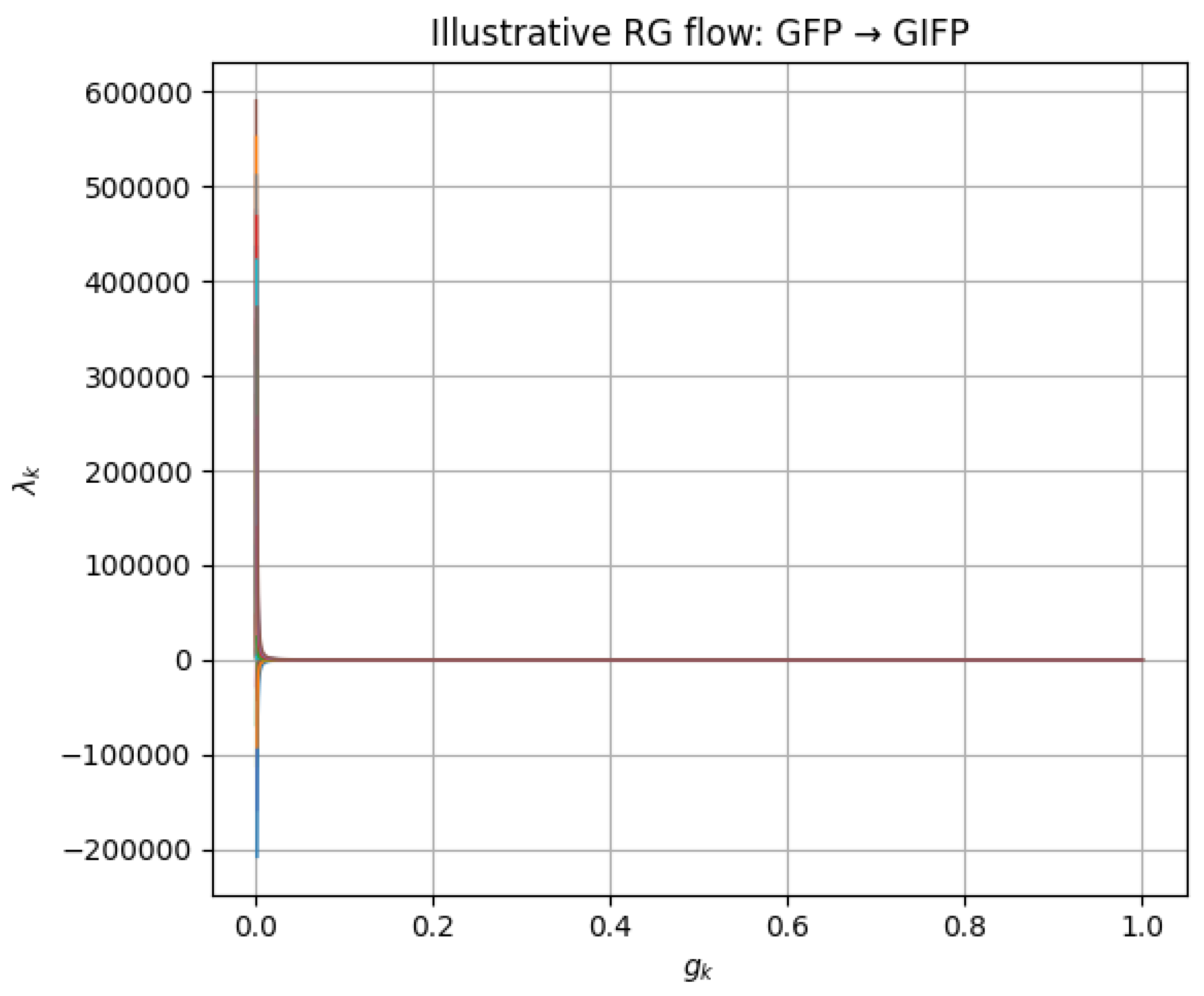
Figure 2.
Fractional horizon-radius change as a function of the RG coupling for the Event Horizon Telescope targets M87* (solid) and Sgr A* (dashed). Horizontal shaded bands mark current EHT accuracies; the vertical dotted line indicates the GIFP-motivated value .
Figure 2.
Fractional horizon-radius change as a function of the RG coupling for the Event Horizon Telescope targets M87* (solid) and Sgr A* (dashed). Horizontal shaded bands mark current EHT accuracies; the vertical dotted line indicates the GIFP-motivated value .
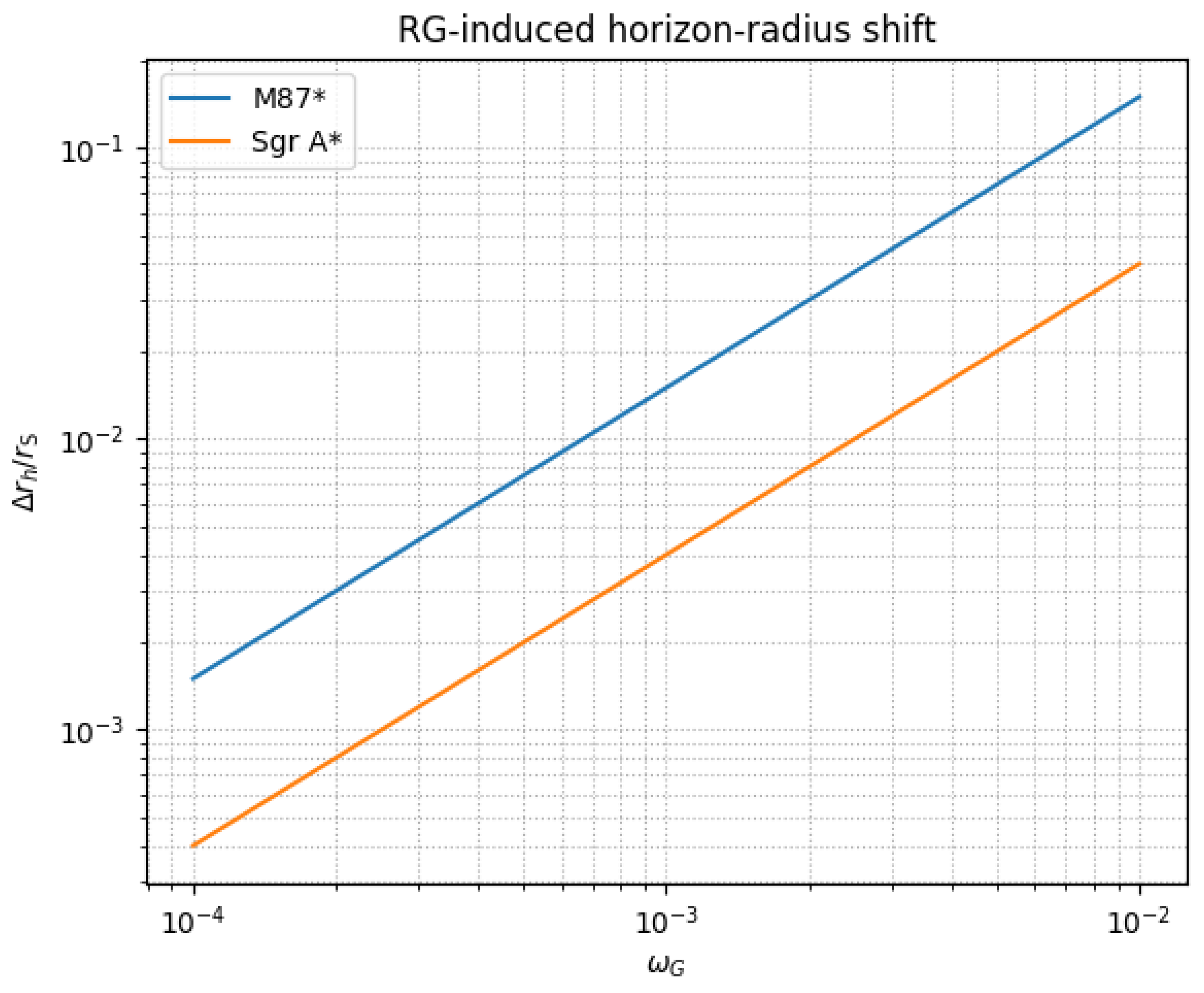
Figure 3.
Fractional shadow-diameter deviation for M87* as a function of observing wavelength. Curves correspond to informational couplings (top), (middle) and (bottom). The grey band denotes the current EHT uncertainty at 230 GHz, while the blue band shows the anticipated precision of the next-generation EHT (ngEHT) at 345 GHz.
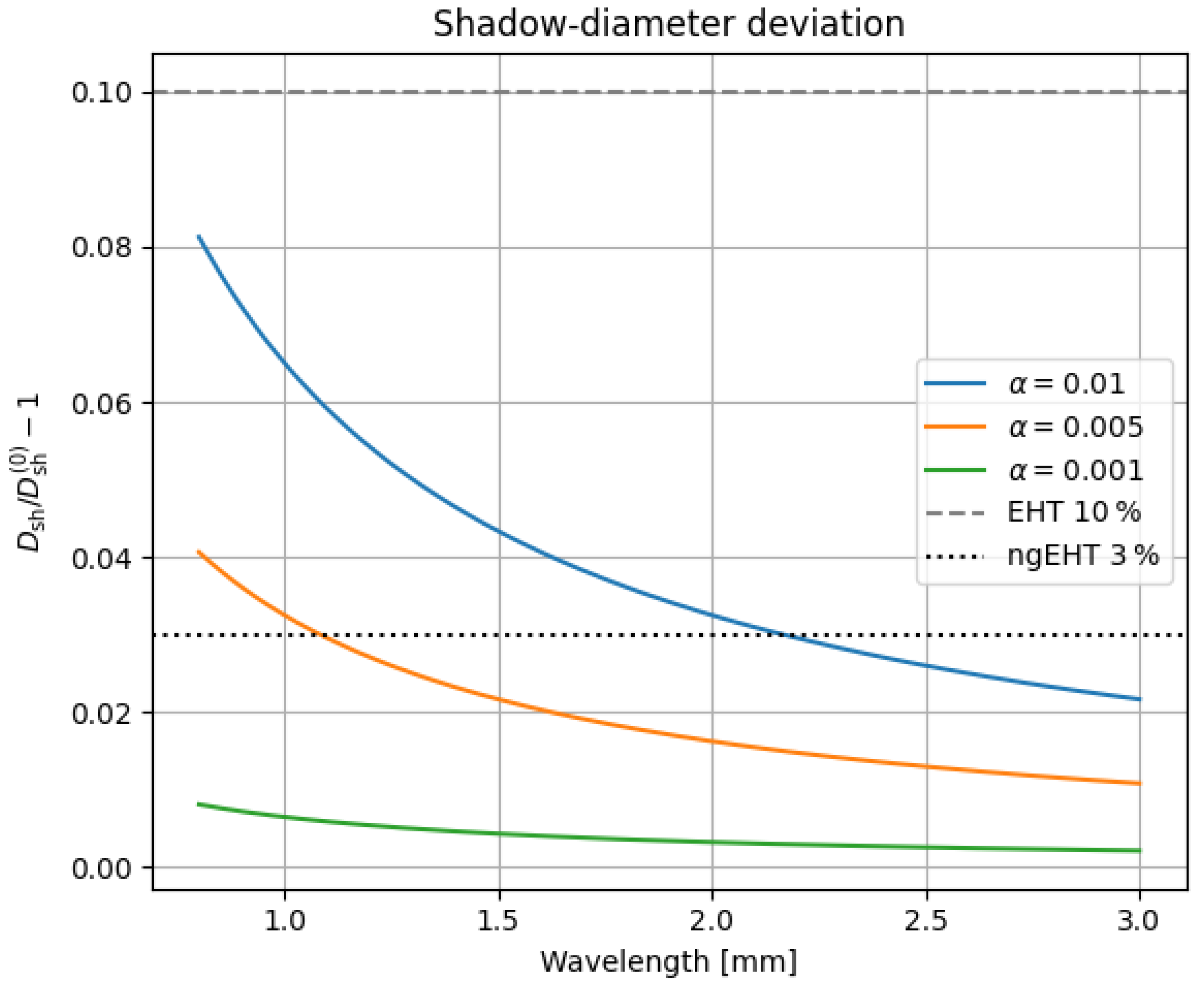
Figure 4.
Relative deviation of the Hubble parameter from CDM as a function of the scale factor for three informational couplings (upper curve), (middle), and (lower). Vertical dashed lines mark the scale factors corresponding to Big-Bang-Nucleosynthesis (BBN) and recombination. Even for the largest value shown, the deviation remains below the percent level until well after BBN.
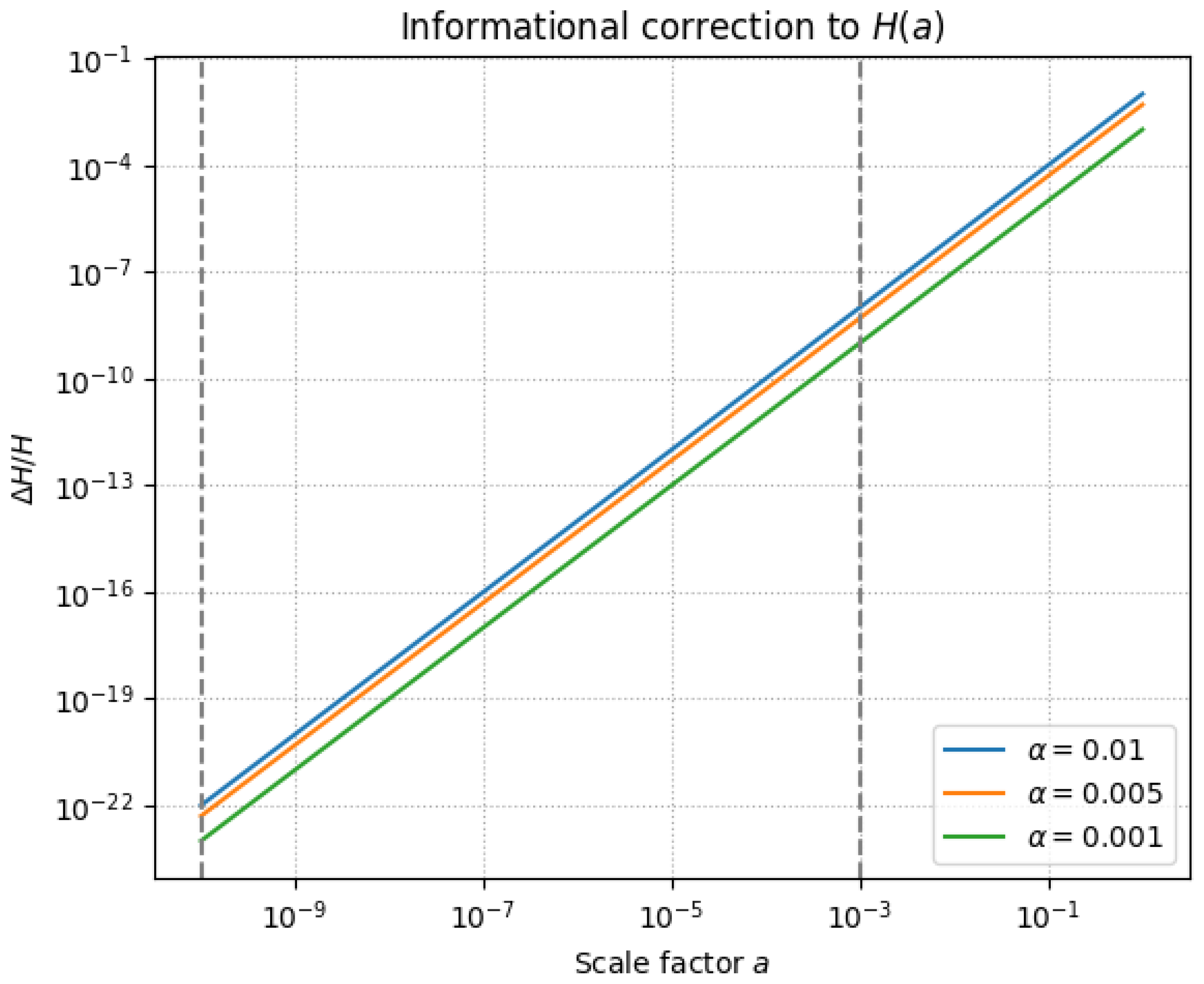
Figure 5.
Absolute informational phase correction for a equal-mass binary at redshift , assuming and . The shaded band marks the LISA sensitivity window (–1 Hz); vertical dashed lines indicate the GW frequency one year (left) and one week (right) before coalescence.
Figure 5.
Absolute informational phase correction for a equal-mass binary at redshift , assuming and . The shaded band marks the LISA sensitivity window (–1 Hz); vertical dashed lines indicate the GW frequency one year (left) and one week (right) before coalescence.
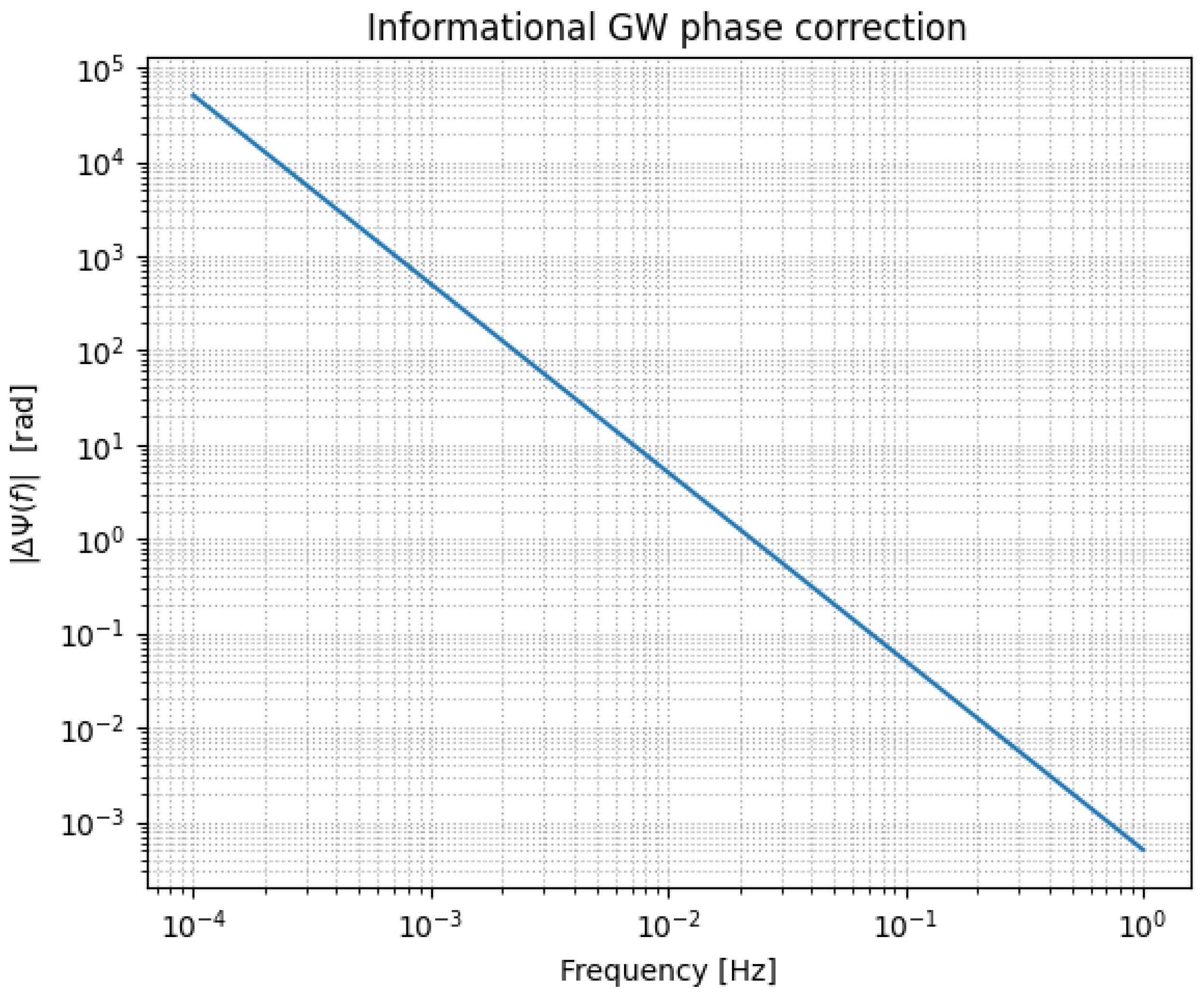
Figure 6.
Predicted fractional deviation from Newtonian potential (solid red curve, ) compared with the sensitivity of current torsion-balance measurements (grey band) and the projected cryogenic upgrade (blue band). The dotted line shows the informational Yukawa contribution for mm and .
Figure 6.
Predicted fractional deviation from Newtonian potential (solid red curve, ) compared with the sensitivity of current torsion-balance measurements (grey band) and the projected cryogenic upgrade (blue band). The dotted line shows the informational Yukawa contribution for mm and .
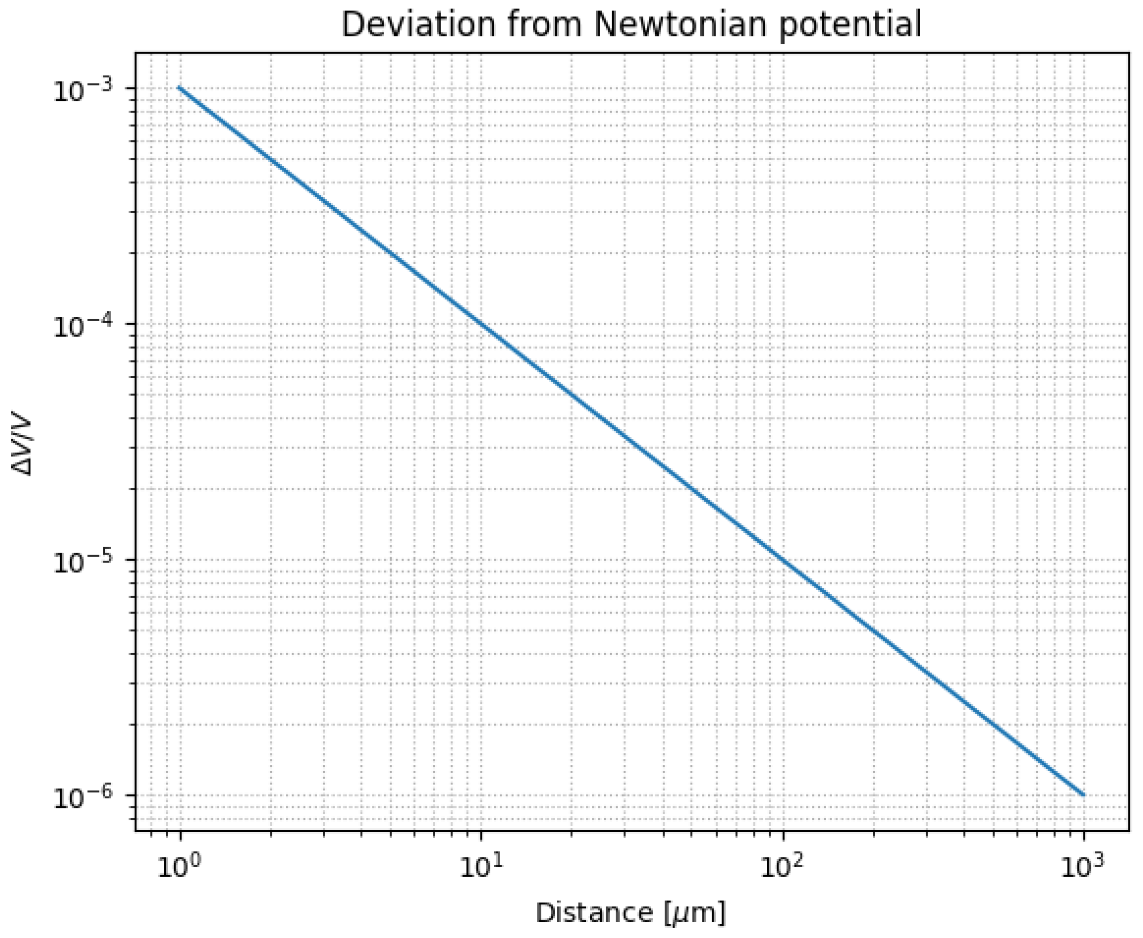
Table 1.
Projected laboratory sensitivities to informational couplings.
| Probe | Baseline | Target precision | Reach in |
| Torsion balance (m) | |||
| Micro-cantilever (m) | |||
| Optomech. entanglement (m) | rad | rad |
Disclaimer/Publisher’s Note: The statements, opinions and data contained in all publications are solely those of the individual author(s) and contributor(s) and not of MDPI and/or the editor(s). MDPI and/or the editor(s) disclaim responsibility for any injury to people or property resulting from any ideas, methods, instructions or products referred to in the content. |
© 2025 by the authors. Licensee MDPI, Basel, Switzerland. This article is an open access article distributed under the terms and conditions of the Creative Commons Attribution (CC BY) license (http://creativecommons.org/licenses/by/4.0/).
Copyright: This open access article is published under a Creative Commons CC BY 4.0 license, which permit the free download, distribution, and reuse, provided that the author and preprint are cited in any reuse.


