
Submitted:
07 May 2025
Posted:
08 May 2025
You are already at the latest version
Abstract
The recording of minerals extracted from a deposit is crucial for effective planning, exploitation management and compliance with legal requirements. It also enables improved workplace safety and minimization of negative environmental impact. Automation in mining optimizes exploitation, transportation, and data management processes, resulting in better forecasting, more accurate resource calculations, and reduced operational costs. Due to the usage of Geographic Information System tools, it facilitates data modelling and analysis, enhancing monitoring and mining exploitation management. This paper presents the classical approach to determining the volume of extracted minerals and proposes the automation of the volume calculation process using GIS tools. The automation of process is presented both from a theoretical perspective, providing requirements and parameters for individual calculation procedures, and from a practical perspective, using the example of a typical open pit mine, where the procedure was implemented starting from field measurements, through calculations, and ending with visualization and interpretation. The study highlights the benefits of automating the calculation procedure for the volume of extracted minerals, including task execution acceleration, increased efficiency, reduced calculation time, and minimized human error. This ultimately leads to more precise and consistent results.
Keywords:
open pit mining
; mineral extraction from the deposit
; volume calculation
; process automation
; GIS
1. Introduction
Mining serves a key role in the development of civilization by providing mineral resources for which the demand is continuously increasing on global markets. In recent decades, technological advancements in the mining industry have occurred in various areas such as the exploration of new deposits, calculation of recoverable reserves, mine design, and the estimation of extracted mineral volumes. Today, the industry faces new technological challenges, including the implementation of advanced automation systems and data analysis methods to enhance productivity and safety. In particular, it involves the use of Geographic Information Systems (GIS) in various tasks that are subject of the daily analytical and computational operations within the mining sector.
GIS is an advanced tool that automates the processes of collecting, storing, retrieving, modifying, evaluating, and presenting georeferencing system [1]. It encompasses geospatial data that describe the spatial position of objects relative to the terrain, as well as attribute data that define the characteristics of these objects. Typically, such data is represented and stored in GIS in either vector or raster format [2]. In vector structures, data appear as points (e.g., mineral occurrences, ground measurements, control points), lines (e.g., faults, fold axes, cross-sections), or polygons (e.g., bedrock boundaries, geological units, surface geology). Conversely, raster data is represented as a grid of cells, where each cell holds an attribute that represents the entire cell area (e.g., Digital Elevation Models—DEMs). The development of GIS has brought significant benefits through the integration of dispersed geological information, facilitating the prediction of mineral deposit occurrences. Overall, the innovative application of geospatial technologies provides effective tools for faster and more efficient data collection, storage, processing, analysis, and presentation [3].
Conventional mineral exploration methods, including the precise determination of deposit volume and value, are carried out utilizing geochemistry, geophysics, traditional geological mapping, photogrammetry, and ground-based surveying. These methods are labor-intensive and complex due to the need to integrate and analyze diverse thematic data. In this context, approach based on remote sensing and GIS is of great practical importance [4].
Underground mining often results in surface deformations, most commonly in the form of so-called subsidence basins, but also discontinuous deformations such as fissures, sinkholes, and scarps. Monitoring of these features with the use of traditional ground-based surveying methods is currently being replaced by remote sensing technologies and GIS systems. Specifically, this type of monitoring is based on electromagnetic waves of various wavelengths in systems such as LiDAR [5], DInSAR [6], and GBInSAR [7] to identify deformation boundaries and quantify them [8]. Basing on various theories regarding the influence of underground mining on surface terrain (e.g., the Knothe-Budryk theory), GIS systems can be used to generate maps predicting terrain deformations [9]. These maps are useful in spatial planning processes, particularly for designing and implementing risk mitigation strategies and management on mining area [10]. In addition to surface deformation (typical of underground mining), other environmental effects such as soil contamination, water pollution, and deforestation (common in open-pit mining) are also recorded and modeled using GIS, making it a valuable tool for addressing mining-induced hazards [11].
For shallow mineral deposits extractable by open-pit technology, GIS-based mine planning research can be divided into four main areas: quantitative mineral resource assessment [12,13,14,15], optimization of open-pit designs [16,17,18,19], mining infrastructure planning [20,21,22], and the analysis of potential conflict areas] [23,24]. In this paper, GIS was applied to automate the calculation of the volume of minerals extracted from an open-pit deposit. The calculation of extracted mineral volume is a part of maintaining a record of deposit resources, which is a component of monitoring and documenting the extraction activities of any mining plant licensed under applicable geological and mining laws.
2. Materials and Methods
To determine the volume of spatial elements, such as mineral deposits or water reservoirs, commonly used is the Boldyrev polygon method, in which the division of surface into polygons is also known in the literature as Voronoi polygons or Thiessen polygons. In mining, this method can be applied both for resource estimation - distinguishing between recoverable (economic) and non-recoverable (uneconomic) resources - and for calculating the volume of minerals extracted from a deposit over a given period, for the purpose of documenting ongoing extraction activities [25]. The data necessary for applying the Boldyrev polygon method include the coordinates of measured points located on the surface of the area under investigation, along with the thickness of the deposit at those points (determined from core sampling) or the thickness of the deposit exploited at these points in the assumed time period (based on geodetic measurements).
In the first stage, the method involves dividing the studied area (within defined boundaries) into polygons. A grid of points is established in the field, with each point’s position determined by measuring its coordinates within the adopted, official coordinate system. The next step is connecting the measurement points with line segments and constructing perpendicular bisectors (Figure 1a). The intersections of these bisectors form the vertices of the polygons (Figure 1a), each of which contains exactly one measurement point. The deposit thickness determined at that point (from core analysis) or the thickness of already extracted material is assumed to represent the height of a right prism whose base is the corresponding polygon (Figure 2b).
Under the provisions of the geological and mining law in force in Poland, as part of the accuracy check of extraction practices at a given mining site, at the end of each calendar year, a document called the resource inventory report is prepared. The inventory report is a document concerning the exploitation of natural resources, including common minerals such as gravel or sand extracted from beneath the water table. It contains data on the quantity of extracted raw materials, measurement methods, environmental impact, and compliance with legal regulations. It serves as evidence during inspections and administrative settlements.
The Boldyrev polygon method (which uses shapes known as Voronoi polygons or Thiessen polygons) can be applied to calculate the volume of minerals extracted from an open-pit mine over the course of a single calendar year [26], what is required for the preparation of the resource inventory report. In such a case, the total volume of extracted material V should be determined at two time points (as of the end of the respective calendar year, denoted as y) using the following formula:
where: n – number of polygons,
hi – height of the i-th right prism,
Ai – area of the i-th polygon.
Having two total volumes of the extracted mineral as of the end of a given calendar year and the end of the following calendar year (a one-year cycle), the difference between these volumes represents the amount of mineral extracted during that calendar year.
In formula (1), the heights of individual rectangular prisms correspond to the thicknesses of the extracted mineral deposit, calculated on the basis of geodetic survey results as the difference between the documented elevation of the top of the deposit (Zupper) and the elevation of the measurement point in a given survey (Zlower).
where: Zupper – elevation coordinate of the upper base of a given polygon,
Zlower–elevation coordinate of the lower base of a given polygon.
The elevation coordinate of the upper base of a given polygon corresponds to the roof elevation of the deposit, which can be obtained from a mining map by reading the elevation of the upper edge of the slope within the deposit. In the case of horizontally layered common mineral deposits, this value is often identical for all polygons. The elevation coordinate of the lower base of a given polygon corresponds to the terrain elevation (in the case of underwater extraction, the bottom elevation of the reservoir) at the time of measurement.
The calculation of the surface area of the polygons is performed automatically using the Gauss–l’Huillier formulas:
where: X, Y – coordinates of the polygon vertices,
k–1, k, k+1 – sequential numbers of the polygon vertices,
m – number of polygon vertices.
This method is commonly used in Poland by mining geologists to calculate documented mineral resources, as well as by mine surveyors to determine the volume of extracted material from deposits during ongoing open-pit mining operations. The main advantage of this method is its universality and accuracy, which depends on the density of the measurement point network. However, the disadvantages include its time-consuming nature and the associated high costs.
In the Boldyrev polygon method (which utilizes Voronoi polygons or Thiessen polygons), the scheme for calculating the volume of material extracted from a deposit over a defined period consists of several stages (Figure 2).
The first stages involve data acquisition related to extraction. This data is obtained through geodetic field measurements. In the case of open-pit mines, topographic and elevation measurements cover the part of the deposit that was subject to extraction during the analyzed period (usually on an annual basis). Measurements are typically carried out using geodetic or photogrammetric techniques, either from the ground or via aerial surveys (e.g., using UAVs). Since most open-pit mines extract common minerals, which are often mined from beneath the water table, measurements in such cases require the use of two complementary techniques: a situational survey (usually conducted with a GPS receiver), and a measure of the depth of the water body (bathymetric survey) [27]. The elevation of the top surface of the mined deposit can be read from a mining map by adopting as the roof level the elevation value of the upper edge of the deposit slope. Subsequent stages comprise of computational procedures aimed at determining the volume of the deposit extracted from the beginning of exploitation at two consecutive time points. Based on this, the volume extracted during a given calendar year is calculated. The individual stages shown in Figure 2 are often carried out through tedious, labor-intensive, and time-consuming calculations. The authors of this study propose using GIS tools to automate these calculations. A flowchart of the procedures implemented in QGIS to determine the volume of material extracted over one year is presented in Figure 3. Yellow blocks represent input data, white blocks represent data operations, and green blocks represent the resulting output data, which serves as the basis for interpretation.
Three vector layers are required as input. Two of these are point layers containing geometry (x, y) and elevation data. The third input layer represents the extraction area in the form of a polygon. It is crucial for all layers to use the same coordinate system - both horizontal and vertical datum. In the case of having data in different coordinate reference systems, they must first be transformed to a common coordinate system through data conversion (coordinate system transformation) before being loaded as input layers.
To test the proposed automated procedure for calculating the volume of extracted mineral, a case study was carried out on a sample open-pit mine extracting common minerals. The process involved collecting field data, analyzing the mining map of the study area, and determining the volume of extracted mineral over the course of a single calendar year.
Field measurements were conducted at a mining site located near Tarnów, Poland (Figure 4a), which extracts common minerals from two open-pit workings, partially located below the groundwater table (Figure 4b).
This site was selected as a representative case study because the majority of mining operations in Poland are conducted using open-pit techniques, and the method of obtaining extraction data is analogous to that presented in this study. This allows the proposed computational procedure to be applied to other open-pit mines as well. Extraction at the studied site is initially carried out using excavators, and once the groundwater level is reached, a dredger is used. The studied excavation site is currently filled with water. During field measurements aimed at, for example, determining the volume of overburden or extracted mineral, a combination of two measurement methods is employed. One regards determining the depth, while the other - identifying the location of the points where the depth measurements are taken [28]. Therefore, measurement of extracted volume at this site requires the simultaneous use of GPS and bathymetric techniques (Figure 4c).
Archival data concerning the morphology of the excavation bottom in the previous year (2023) were obtained in the form of an analog mining map with elevation data marked at the measurement points. A follow-up survey was scheduled one year later, involving approximately 80 measurement points evenly distributed across the reservoir surface. Measurements were conducted by simultaneously recording data from a GPS receiver and an echo sounder when the boat was stationary, ensuring precise recording of both the coordinates and the depth. The engine was turned off, and the boat was allowed to settle to ensure accurate and reliable three-dimensional readings. Measurements were performed from a floating vessel using a Hi-Target H32 GPS receiver and a Humminbird Sonar 718 echo sounder.
3. Results
By subtracting the depths measured with the echo sounder from the water surface elevation, the bottom elevations of the excavation (Z) were obtained. These were then compiled together with the coordinates (X, Y) recorded using the GPS measurement. The resulting dataset, containing X, Y, and Z coordinates expressed in meters, was exported to a .csv file to enable its import into the QGIS software as an attribute table of a point layer (Figure 5).
The X and Y coordinates were determined in the [PUWG 2000] system with a mean error not exceeding a few centimeters, while the elevation values were referenced to the [Kronstadt 86] vertical datum, consistent with archival measurements from the previous year (2023), with an accuracy of ±10 cm (as specified by the equipment manufacturer). In QGIS, the appropriate columns were assigned as geographic coordinates, with the EPSG:2178 (ETRF2000-PL/CS2000/21) reference system selected. Due to differences between the Polish national coordinate system [(PUWG 2000)] and the Cartesian coordinate system used by the software, it was necessary to swap the X and Y coordinates. To verify the correctness of the data, they were displayed on a satellite map background with labels (Figure 6), which also included the extraction area as a polygon.
The next step was obtaining data to create a point layer based on measurements from the previous year. For this purpose, archival data, a scanned topographic map from the previous year (2023) was digitized. Using the Georeferencer tool in QGIS, georeferencing was applied to the image (the scanned analog map). Characteristic points were identified on the raster image, specifically a grid of crosses spaced at 100-meter intervals. After selecting all points, the transformation method that produced the lowest mean error was chosen. A third-degree polynomial was selected, resulting in an error of 1.29 meters, along with the nearest neighbor resampling method. Once the algorithm was applied, all points measured in 2023 within the reservoir area were transferred to new vector layers, along with its boundaries, based on the lower edge of the slope within the deposit.
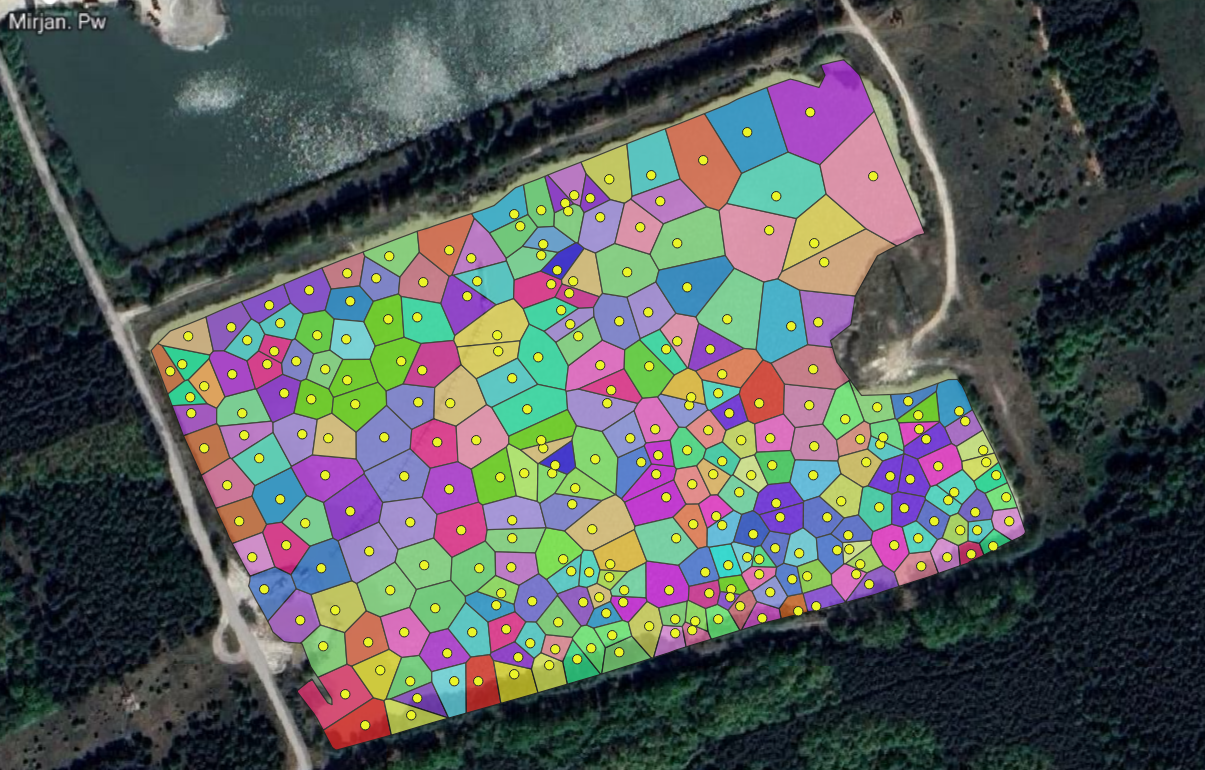
Having two point layers - one from 2023 and the other from 2024 - as well as a polygon layer, the automated procedures described and outlined in Figure 3 were initiated. First, Voronoi polygons were created for both point layers using the “Create Voronoi Polygons” function. This function generates Voronoi polygons based on the input point layer, with the result shown in Figure 7. The characteristics of the “Create Voronoi Polygons” procedure are presented in Table 1. It is possible to apply a buffer to extend the extent of the output layer, set a snapping tolerance to speed up the algorithm, and choose whether to retain (copy) the attributes from the input layer into the output layer.
The “Create Voronoi Polygons” procedure was applied to both the 2023 and 2024 point layers. In the next step, the resulting Voronoi polygon layers were clipped to the boundaries of the overlaid polygon layer representing the outline of the open-pit excavation area. For this purpose, the “Clip Polygons to Area” tool was used (Figure 8).
In the „Clip polygons to area” operation, an intersection between a colourful multi-feature input layer and a gray single-feature overlay layer takes place (Figure 8 left). As a result, overlapping areas become a new layer with attributes from the first layer (Figure 8 right). To use the “Clip polygons to area” operation, it is required to provide as INPUT any vector layer to be clipped and a polygon vector layer defining the clipping area. The OUTPUT is a vector layer of the same type as the first INPUT layer. The result of applying the “Clip polygons to area” operation is shown in Figure 9.
In the next procedure, “Intersection,” the overlapping areas between objects from the input layer and the overlay layer are determined. The input layer in this case is the vector layer with polygons from the previous year (2023), visualized in a color scale ranging from blue to red. The overlay layer is the polygon layer from the following year (2024), displayed as edges of all polygons (Figure 10). The requirements and parameters for the “Intersection” procedure are presented in Table 2.
The calculation of the extracted mineral volume was carried out using the “Calculate volumes” procedure for each layer - that is, for each of the polygons generated from the 2023 data (Figure 9), and analogously for each polygon created from the 2024 data. In this procedure, the field calculator is used to compute the volume value for each feature in the layer. The requirements and parameters for the “Calculate volumes” procedure are presented in Table 3.
Grouping objects according to specific criteria or calculating statistical values for layers is done using another function in the flow chart (Figure 3) called “Aggregate volumes”. This function uses mandatory arguments such as: “layer” (layer name), “aggregate” (aggregation type, e.g., sum, average, minimum, maximum), “expression” (expression or field to aggregate), and optional arguments: “filter” (condition limiting data for aggregation), “concatenator” (connector for aggregated text values), and “order by” (defining the order of aggregated expressions or fields).
The volume calculation for the annual cycle in the 2023–2024 period was done using the “Subtract sum of volumes” function, which provides a single final result. The arguments for this function are: “volume 1” (the sum of the volume of material extracted in the first year) and “volume 2” (the sum of the volume of material extracted in the second year). The expression for calculations returns the result as a decimal number.
In the used method, upper edge of the slope in the deposit was adopted as the reference level. By subtracting the volume measured in 2023 from that of 2024, the extracted volume for the period was obtained. The volume calculation for both measurement sessions using the field calculator required applying an algorithm that calculated volumes by multiplying the difference between the average roof of the deposit (186.6m above sea level) and the floor elevation by the surface area of the polygon. The total volume for 2023 was 16,521,570.3 m³, and for 2024 it was 16,527,924.7 m³. The difference between these values, which is 6354.4 m³, represents the extracted volume of material.
Analyzing the automation of the calculation process presented in the diagram Figure 3, the output consists of 3 polygon vector layers and one number. By properly applying styles and symbols, the resulting layers: “polygons-year 1” (Figure 11), “polygons-year 2” (Figure 12) and “intersection of polygons and polygons 2” (Figure 13), can serve for the graphical interpretation of changes in the morphology of the floor.
Differential elevation map (Figure 13) enables the visualization of terrain changes. Negative values indicate a decrease in bottom elevation, meaning that extraction has occurred, while positive values indicate an increase in bottom elevation. In Figure 13, near the southern edge, there is an area where elevation values have increased. The same area in Figure 12 is characterized by a high elevation gradient. It can be assumed that these changes are the result of material movement from the shore toward the deeper part of the excavation along a steep slope. This knowledge provides the opportunity to forecast further changes, monitor them, or even prevent them.
The value of 6354.4 m³, obtained through a sequence of calculations and result aggregation, represents the volume of mineral extracted from the deposit over the one-year period (2023–2024). This final result fulfills the initial objective of automating the calculation process.
4. Discussion
The daily operations of mineral extraction at a mining site are supported not only by miners but also by specialists in fields such as geology and mine surveying. As part of their duties, these professionals record the volume of extracted material in documents known as resource inventory reports. The preparation of such report is preceded by field surveys, which, in the case of open-pit mines, aim to create a topographic map of the pit floor. Bathymetric measurements using an echo sounder in conjunction with GPS are essential for generating an up-to-date map of the mined area when extraction takes place below the water table. The results of these measurements, once processed, analyzed, and compared with previous data, are used in the preparation of the inventory report.
The calculation of the volume of extracted mineral is the final stage of the deposit balance documentation. The Boldyrev Polygon method allows for accurate volume determination based on field data. Depending on the purpose for which the method is applied (resource estimation/extraction volume calculation), it requires data on the location of measurement points and the thickness of the deposit or extracted material at those points. In the case of extraction below the water table, the volume is determined by dividing the pit floor into polygons, constructing prisms based on these polygons, and calculating the volume of each prism up to the reference level ( roof of the deposit). The total extracted volume is obtained by summing the volumes of all prisms. The annual extraction volume is determined by comparing the total deposit volumes calculated at two different time points using formula (1). The difference between these values represents the amount of mineral extracted over the course of one year. The final report includes all required information and is submitted to the relevant authorities both at the end of each calendar year and after the completion of mining operations.
Given the widespread use of the Boldyrev Polygon method for volume calculations, despite its shortcomings related to the high demand for measurement and computational work, the authors undertook the task of analyzing individual stages of the process with the aim of automating it using GIS tools. This automation was demonstrated using a typical example of a mining operation extracting common mineral resources under conditions where excavation occurs below the water table. This case was selected due to the prevalence of such mining operations, which means that beyond the scientific aspect, the developed automation process has significant practical relevance, as it can be applied by numerous professionals in the fields of geology and mine surveying.
For the analyzed open-pit excavation site, the volume of mineral extracted in 2024 was calculated using the Boldyrev Polygon method with the automation of computational procedure. A novel approach was proposed involving the use of digital QGIS tools, both for calculations and for the graphic presentation of the mineral volume determination process. The upper edge of the deposit slope was adopted as the reference level for calculating the volumes of individual prisms. By subtracting the 2023 volume from the 2024 volume, the amount of mineral extracted over the one-year period was determined to be 6354.4 m³. In the case of the analyzed mining operation, which holds a concession issued by the governor (in accordance with local geological and mining law), the maximum permitted annual extraction volume is 10000 m³. Based on the calculated volume, it can be concluded that the entrepreneur did not exceed the limit specified in the concession. It is also important to note that this example is illustrative, and the accuracy of the calculated volume can be improved by increasing the number of measurement points - a factor which, in the case of an automated process, is mostly irrelevant to the computational time.
The models and cartographic studies developed using the automated GIS tools presented in this paper may become a key element of analysis not only during the extraction of mineral resources but also after mining operations have concluded (e.g., for reclamation planning purposes). The modeling results presented in graphical form make interpretation easier and faster, especially in terms of comparing with earlier stages of extraction. The use of software related to spatial information systems and modeling will certainly contribute to the advancement of hydrology. Due to the end of exploitation, hypsometric maps and bottom models will be useful in the reservoir reclamation process. In the case of water reclamation, control involves determining slope values above and below the water surface, which must not exceed threshold values. The developed materials can additionally support this process.
Author Contributions
Conceptualization, A.S.; methodology, A.S. and M.S.; software, M.S..; validation, A.S. and M.S.; formal analysis, A.S. and M.S.; investigation, A.S. and M.S.; resources, A.S.; data curation, A.S.; writing—original draft preparation, A.S. and M.S.; writing—review and editing, A.S.; visualization, M.S.; supervision, A.S.; project administration, A.S.
Funding
This research received no external funding.
Data Availability Statement
The data presented in this study are available on request from the corresponding author.
Conflicts of Interest
The authors declare no conflicts of interest.
References
- Bolstad, P. GIS Fundamentals, A First Text on Geographic Information Systems, 6th ed.; Bolstad, P., Ed.; Xan Edu Publishing Inc.: Livonia, MI, USA, 2019; pp. 1–764. [Google Scholar]
- Zhou, G.; Pan, Q.; Yue, T.; Wang, Q.; Sha, H. Vector and raster data storage based on Morton code. Proceedings of The ISPRS TC III Mid-term Symposium “Developments, Technologies and Applications in Remote Sensing”, Beijing, China, 7–10 May 2018. [Google Scholar]
- Omali, T.U. Utilization of Remote Sensing and GIS in Geology and Mining. Int. J. Sci. Res. Multidiscip. Stud. 2021, 7(4), 17–24. [Google Scholar]
- Desheng, Y.; Gang, C.; Xiaoping, L. Application of geological interpretation and mineralization information extracting by remote-sensing in mineral resource evaluating. J. Editor. Board HPU (Natl. Sci. ) 2010, 29, 184–189. [Google Scholar]
- Puniach, E.; Gruszczyński, W.; Ćwiąkała, P.; Matwij, W. Application of UAV-based orthomosaics for determination of horizontal displacement caused by underground mining. ISPRS J. Photogramm. Remote Sens. 2021, 174, 282–303. [Google Scholar] [CrossRef]
- Guzy, A.; Łucka, M.; Witkowski, W. Advancing InSAR Applications in Detecting Land Movement and Sinkhole Precursors in Post-Mining Landscapes. In Proceedings of the EGU General Assembly, Vienna, Austria, 14–19 April 2024. [Google Scholar] [CrossRef]
- Szafarczyk, A. Kinematics of mass phenomena on the example of an active landslide monitored using GPS and GBInSAR technology. J. Appl. Eng. Sci. 2019, 17(2), 107–115. [Google Scholar] [CrossRef]
- Behera, A.; Rawat, K.S. A Comprehensive Review on Mining Subsidence and its Geo-environmental Impact. Journal of Mines, Metals and Fuels 2023, 71(9), 1224–1234. [Google Scholar] [CrossRef]
- Suh, J. An Overview of GIS-Based Assessment and Mapping of Mining-Induced Subsidence. Appl. Sci. 2020, 10, 7845. [Google Scholar] [CrossRef]
- Malinowska, A.; Hejmanowski, R. Building damage risk assessment on mining terrains in Poland with GIS application. Int. J. Rock Mech. Min. Sci. 2010, 47(2), 238–245. [Google Scholar] [CrossRef]
- Suh, J.; Kim, S.M.; Yi, H.; Choi, Y. An Overview of GIS-Based Modeling and Assessment of Mining-Induced Hazards: Soil, Water, and Forest. Int J Environ Res Public Health. 2017, 14(12), 1463. [Google Scholar] [CrossRef]
- Sprague, K.; de Kemp, E.; Wong, W.; McGaughey, J.; Perron, G.; Barrie, T. Spatial targeting using queries in a 3-D GIS environment with application to mineral exploration. Comput. Geosci. 2006, 32, 396–418. [Google Scholar] [CrossRef]
- Uygucgil, H.; Konuk, A. Reserve estimation in multivariate mineral deposits using geostatistics and GIS. J. Min. Sci. 2015, 51, 993–1000. [Google Scholar] [CrossRef]
- Hosseinali, F.; Alesheikh, A.A. Weighting Spatial Information in GIS for Copper Mining Exploration. Am. J. Appl. Sci. 2008, 5, 1187–1198. [Google Scholar] [CrossRef]
- Kim, S.M.; Choi, Y.; Park, H.D. New Outlier Top-Cut Method for Mineral Resource Estimation via 3D Hot Spot Analysis of Borehole Data. Minerals 2018, 8, 348. [Google Scholar] [CrossRef]
- Baek, J.; Choi, Y.; Park, H.-S. Uncertainty Representation Method for Open Pit Optimization Results Due to Variation in Mineral Prices. Minerals 2016, 6, 17. [Google Scholar] [CrossRef]
- Sinha, N.; Deb, D.; Pathak, K. Development of a mining landscape and assessment of its soil erosion potential using GIS. Eng. Geol. 2017, 216, 1–12. [Google Scholar] [CrossRef]
- Grenon, M.; Hadjigeorgiou, J. Integrated structural stability analysis for preliminary open pit design. Int. J. Rock Mech. Min. 2010, 47, 450–460. [Google Scholar] [CrossRef]
- Grenon, M.; Laflamme, A.-J. Slope orientation assessment for open-pit mines, using GIS-based algorithms. Comput. Geosci. 2011, 37, 1413–1424. [Google Scholar] [CrossRef]
- Lechner, A.M.; Devi, B.; Schleger, A.; Brown, G.; McKenna, P.; Ali, S.H.; Rachmat, S.; Syukril, M.; Rogers, P. A Socio-Ecological Approach to GIS Least-Cost Modelling for Regional Mining Infrastructure Planning: A Case Study from South-East Sulawesi, Indonesia. Resources 2017, 6, 7. [Google Scholar] [CrossRef]
- Blachowski, J. Spatial analysis of the mining and transport of rock minerals (aggregates) in the context of regional development. Environ. Earth Sci. 2014, 71, 1327–1338. [Google Scholar] [CrossRef]
- Baek, J.; Choi, Y. A New Method for Haul Road Design in Open-Pit Mines to Support Ecient Truck Haulage Operations. Appl. Sci. 2017, 7, 747. [Google Scholar] [CrossRef]
- Preciado, J.R.; Rap, E.; Vos, J. The politics of Land Use Planning: Gold mining in Cajamarca, Peru. Land Use Policy 2015, 49, 104–117. [Google Scholar] [CrossRef]
- Craynon, J.R.; Sarver, E.A.; Ripepi, N.S.; Karmis, M.E. AGIS-based methodology for identifying sustainability conflict areas in mine design—A case study from a surface coal mine in the USA. Int. J. Min. Reclam. Environ. 2016, 30, 197–208. [Google Scholar] [CrossRef]
- Jurys, L.; Damrat, M. Problems of reserves inventorying and calculating the volume of extraction on the example of aggregates deposits. Górnictwo odkrywkowe 2019, 1, 18–24. [Google Scholar]
- Nieć, M.; Mucha, J.; Sobczyk, E.; Wasilewska-Błaszczyk, M. Część IV Szacowanie zasobów. In Metodyka dokumentowania złoż kopalin stałych; Nieć, M., Ed.; Instytut Gospodarki Surowcami Mineralnymi i Energią PAN: Kraków, Polska, 2012; pp. 1–229. [Google Scholar]
- Szafarczyk, A.; Gawałkiewicz, R. An inventory of opencast mining excavations recultivated in the form of water reservoirs as an example of activities increasing the retention potential of the natural environment: a case study from Poland. Geology, Geophysics and Environment. 2023, 49(4), 401–418. [Google Scholar] [CrossRef]
- Jurys, L.; Maszloch, E.; Uścinowicz, G.; Wirkus, K. Analiza dokładności szacowania zasobów i średnich parametrów złóż kruszyw na dnie Bałtyku na podstawie danych z dokumentacji “Ławica Słupska”, Południowa Ławica Środkowa”, Zatoka Koszalińska” oraz „Zatoka Gdańska I” i “Zatoka Gdańska II”. Górnictwo Odkrywkowe 2022, 1(1), 33–38. [Google Scholar] [CrossRef]
Figure 1.
Principle of calculating deposit volume using the Boldyrev polygon method a) Construction of a polygon by drawing perpendicular bisectors of line segments connecting measurement points b) Right prisms with heights corresponding to the deposit thickness at each point.
Figure 1.
Principle of calculating deposit volume using the Boldyrev polygon method a) Construction of a polygon by drawing perpendicular bisectors of line segments connecting measurement points b) Right prisms with heights corresponding to the deposit thickness at each point.
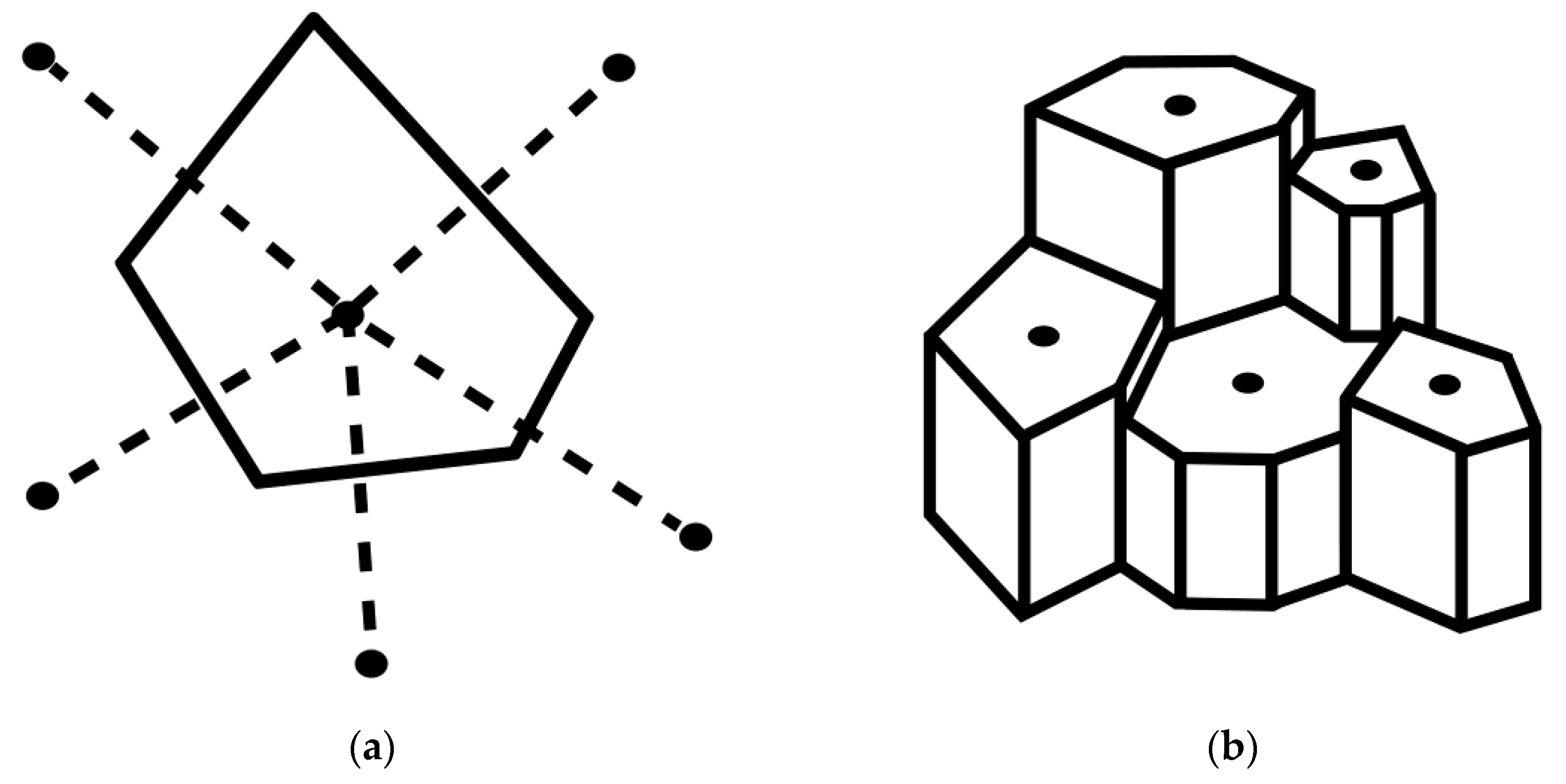
Figure 2.
Diagram of the calculation of the volume of minerals extracted from beneath the water table over the course of one calendar year.
Figure 2.
Diagram of the calculation of the volume of minerals extracted from beneath the water table over the course of one calendar year.
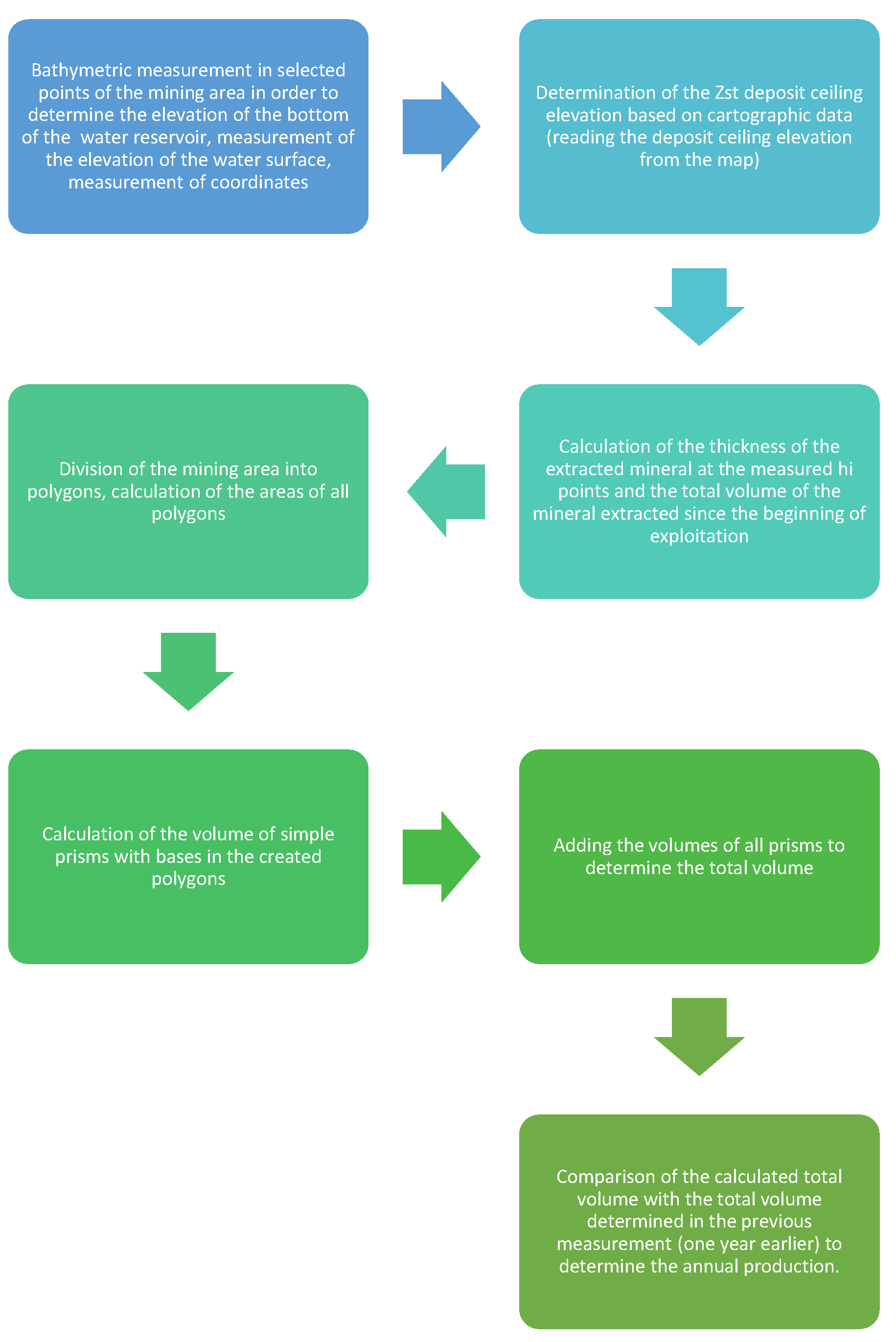
Figure 3.
Automation of the process for determining the volume of mineral extracted over the course of one year. Flowchart of procedures carried out in QGIS.
Figure 3.
Automation of the process for determining the volume of mineral extracted over the course of one year. Flowchart of procedures carried out in QGIS.
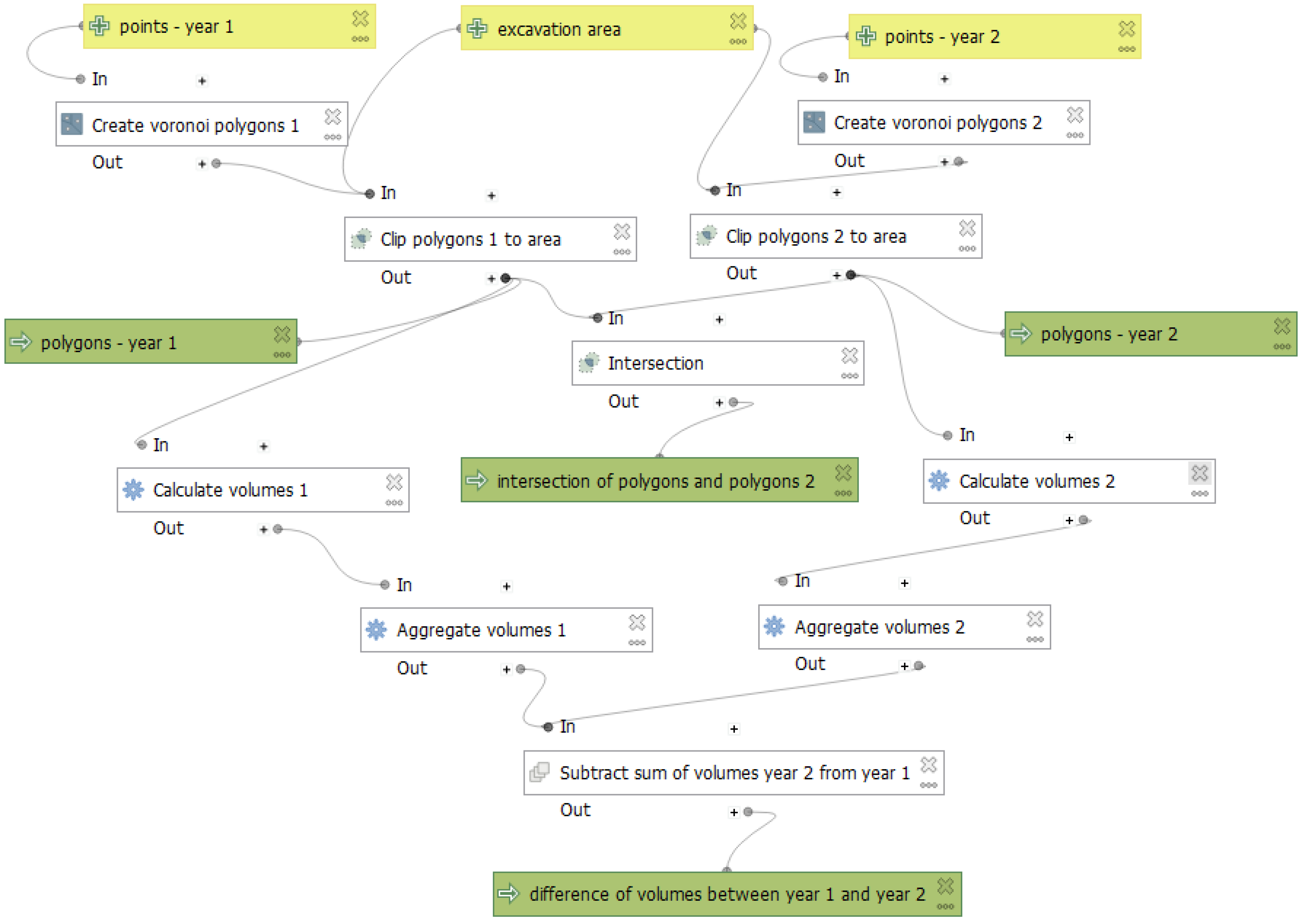
Figure 4.
Location of the Ruda-Borowiec reservoir, where bathymetric measurements were conducted to calculate the volume of extracted minerals (a), (b) own work based on maps from Geoportal.gov.pl), (c) photo: A. Szafarczyk.
Figure 4.
Location of the Ruda-Borowiec reservoir, where bathymetric measurements were conducted to calculate the volume of extracted minerals (a), (b) own work based on maps from Geoportal.gov.pl), (c) photo: A. Szafarczyk.
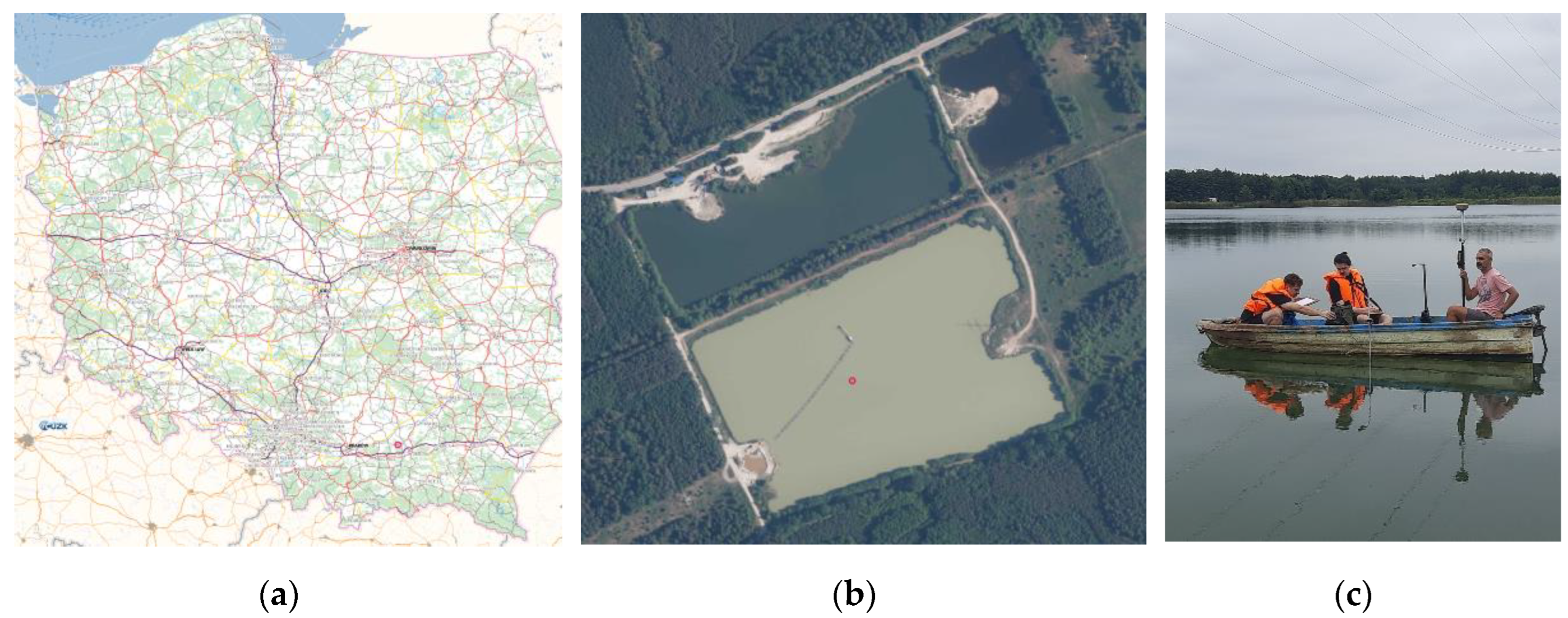
Figure 5.
Fragment from the attribute table of the point layer prepared in QGIS.
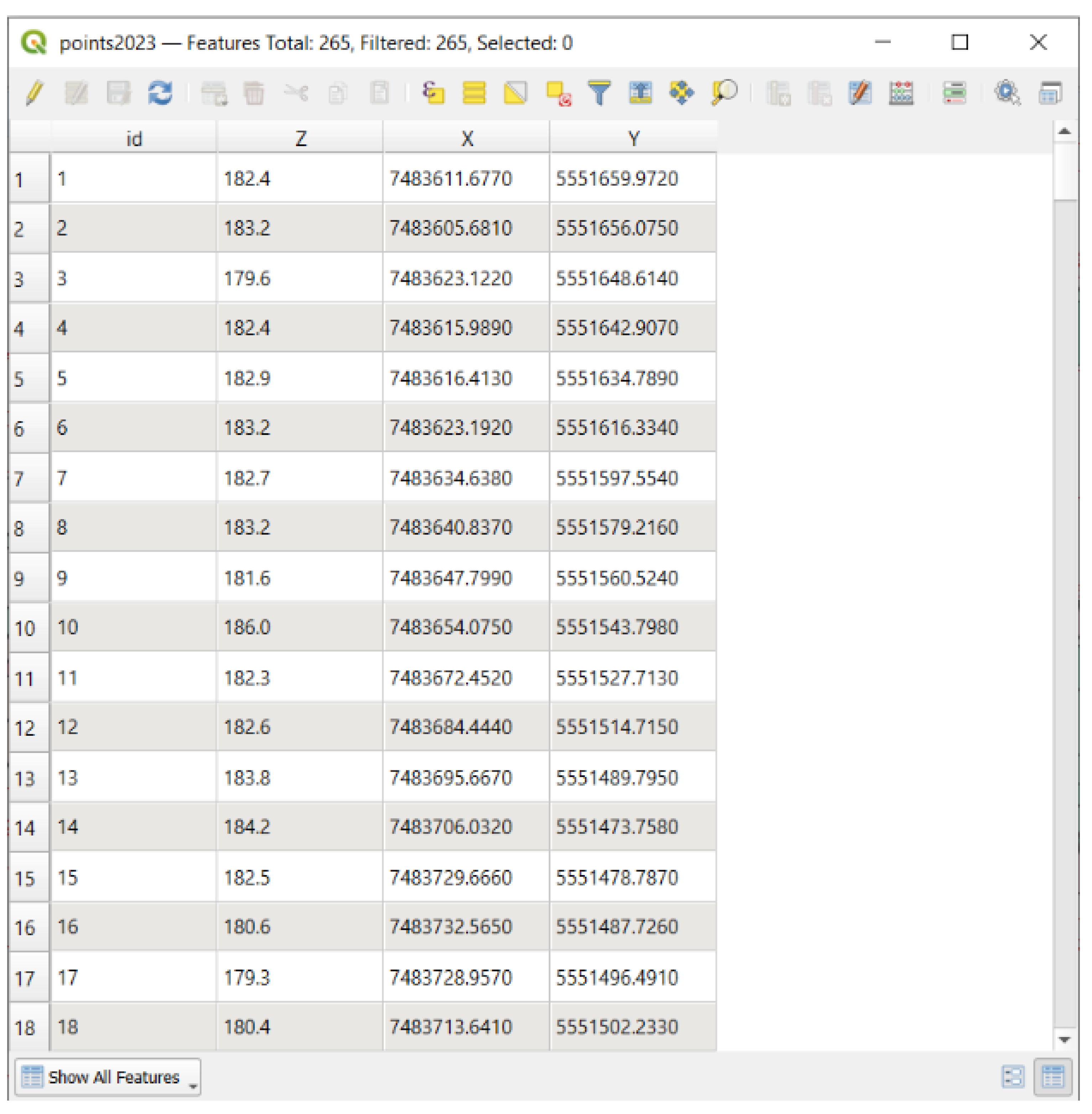
Figure 6.
Vector layers: points and polygon on a Google Satellite map background.
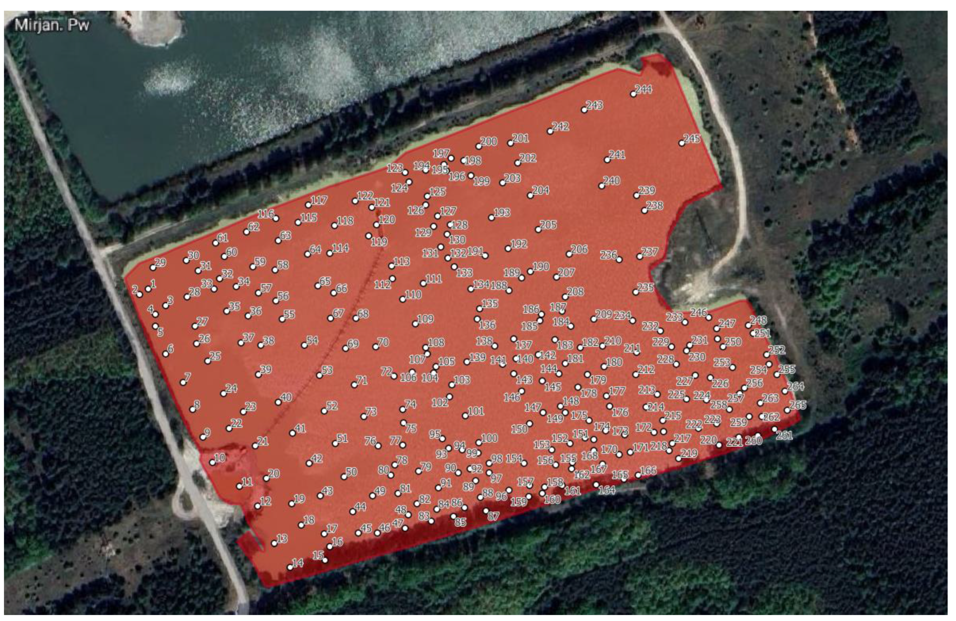
Figure 7.
Point layer and the result of the Create Voronoi Polygons procedure displayed on a Google Satellite map background.
Figure 7.
Point layer and the result of the Create Voronoi Polygons procedure displayed on a Google Satellite map background.
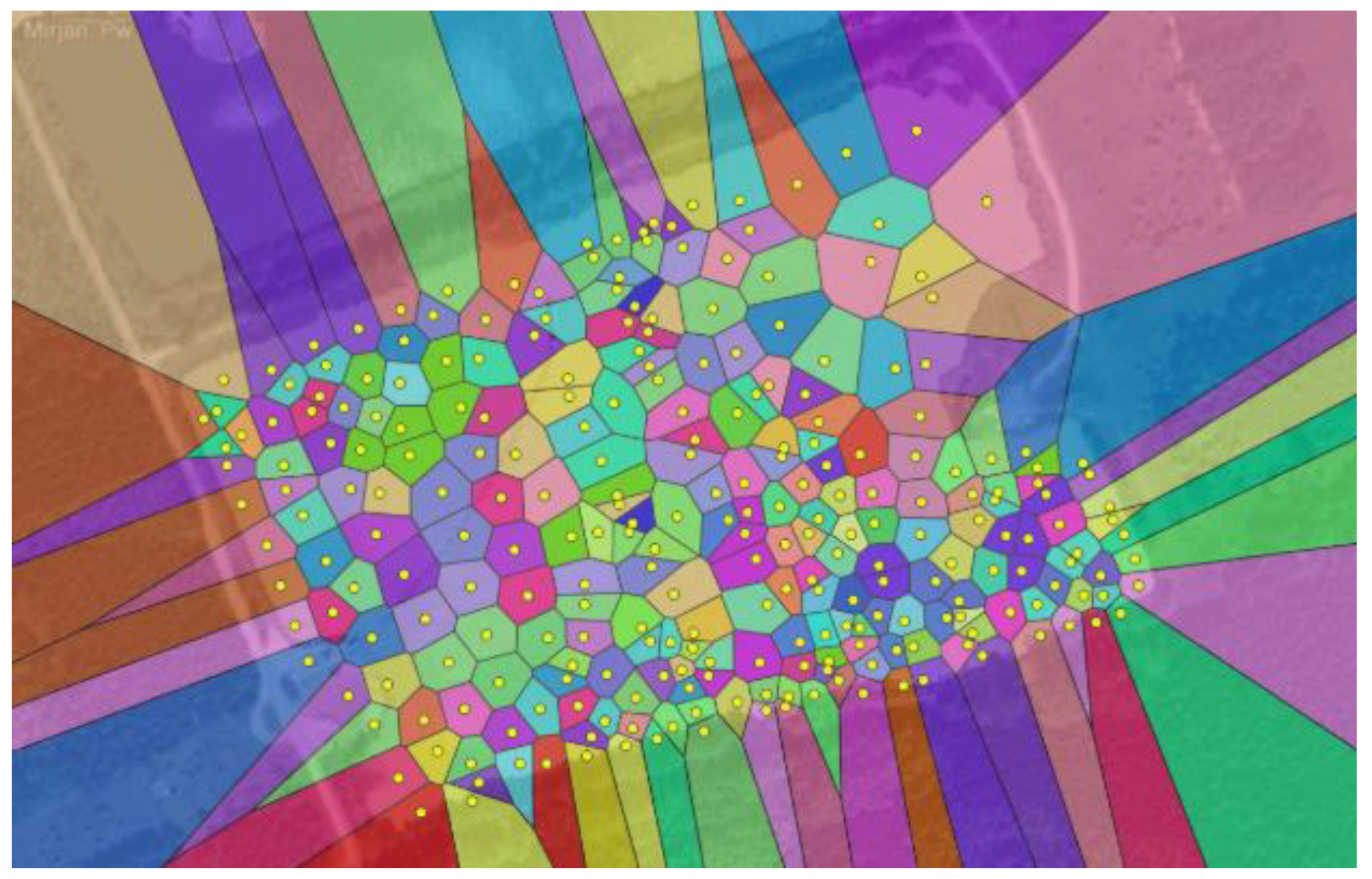
Figure 8.
Principle of the “Clip polygons to area” operation.
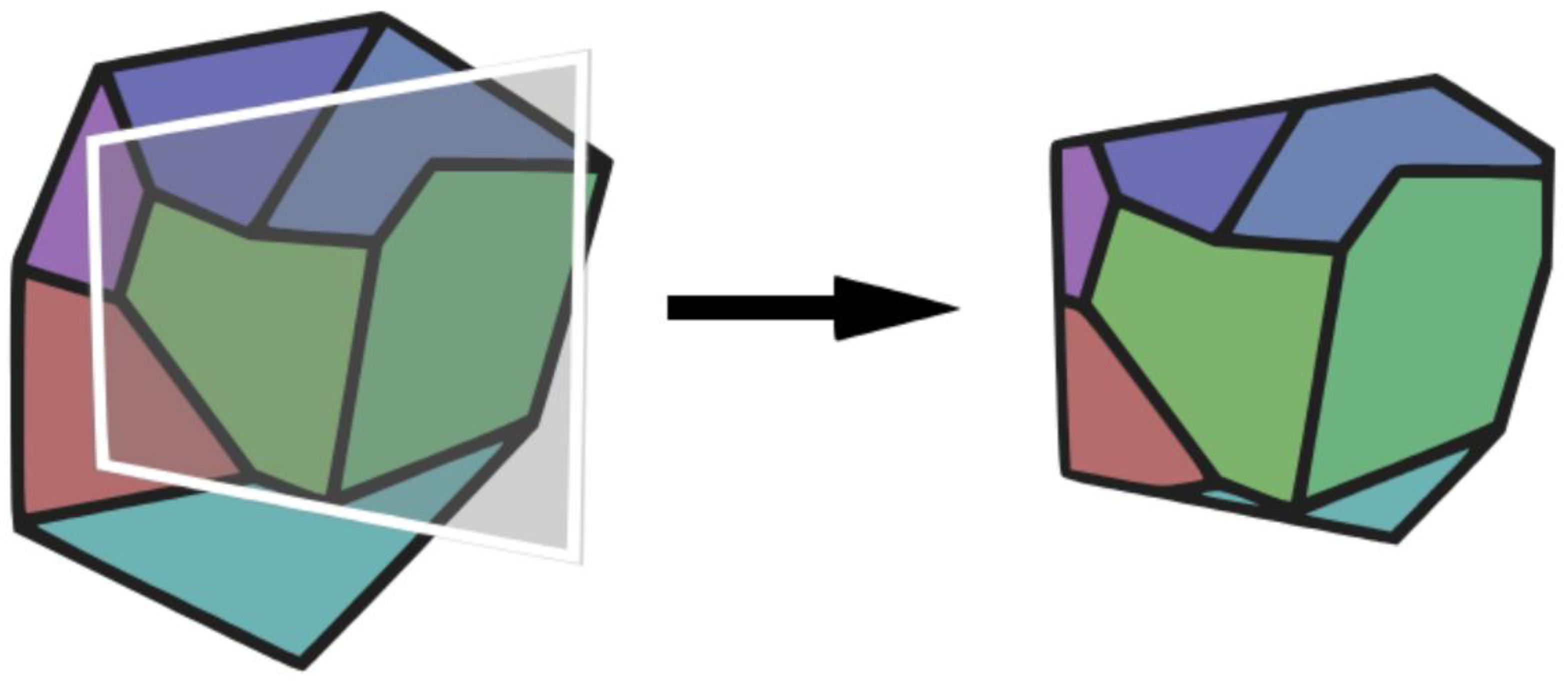
Figure 9.
Point layer and the result of the “Clip polygons to area” procedure displayed on the Google Satellite map background.
Figure 9.
Point layer and the result of the “Clip polygons to area” procedure displayed on the Google Satellite map background.
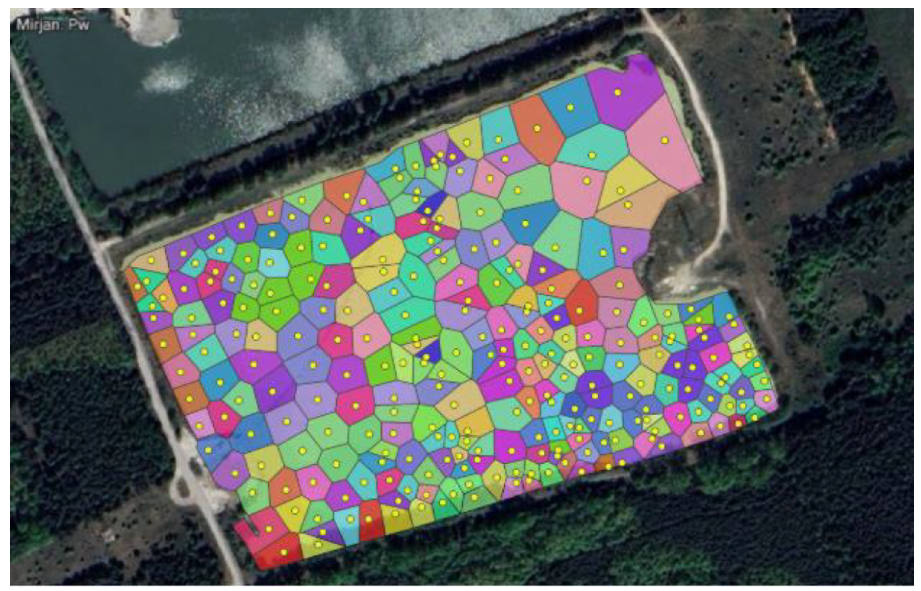
Figure 10.
Layers used in the “Intersection” procedure displayed on a Google Satellite map background.
Figure 10.
Layers used in the “Intersection” procedure displayed on a Google Satellite map background.
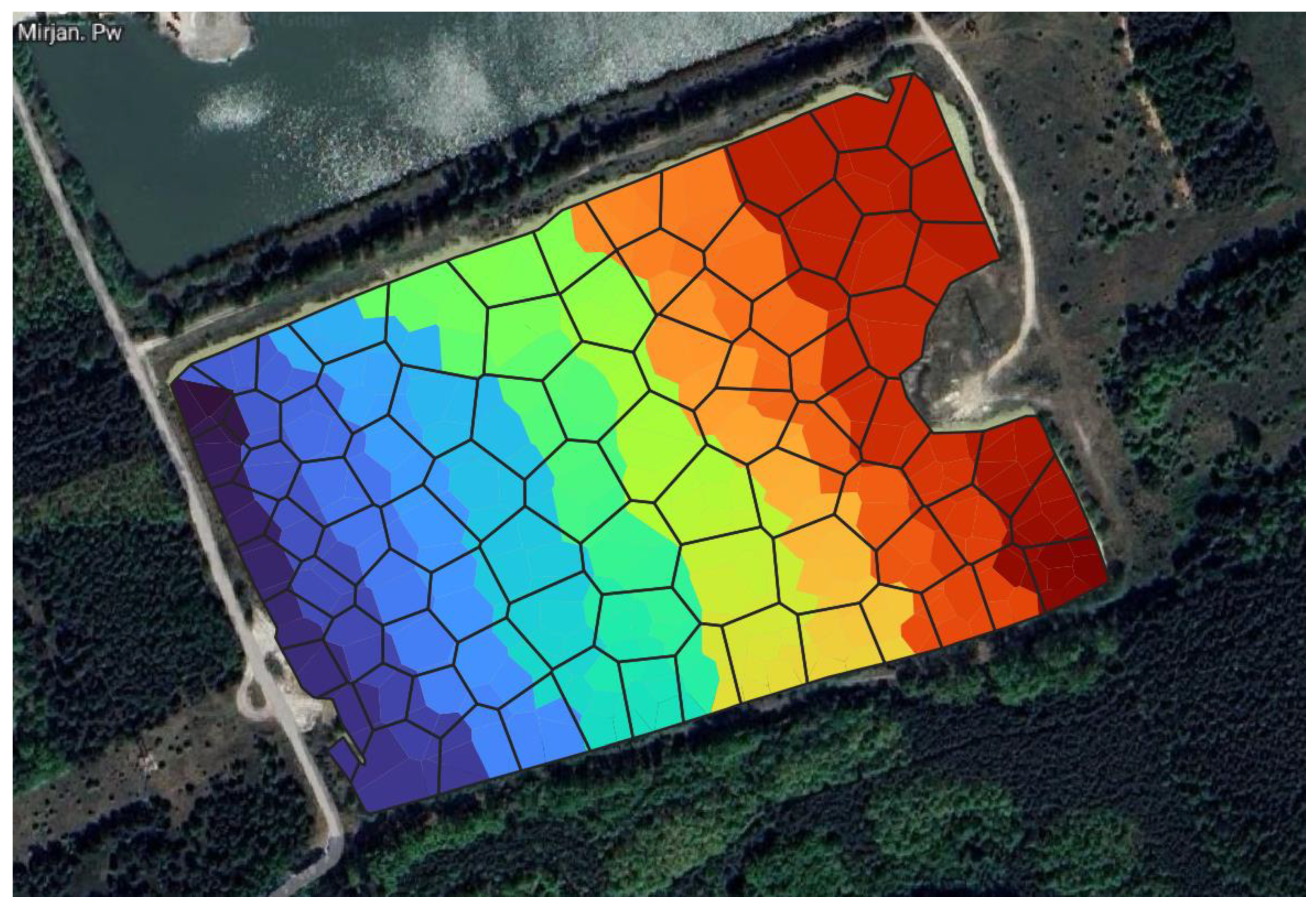
Figure 11.
Output layer “polygons – year 1” with applied styles.
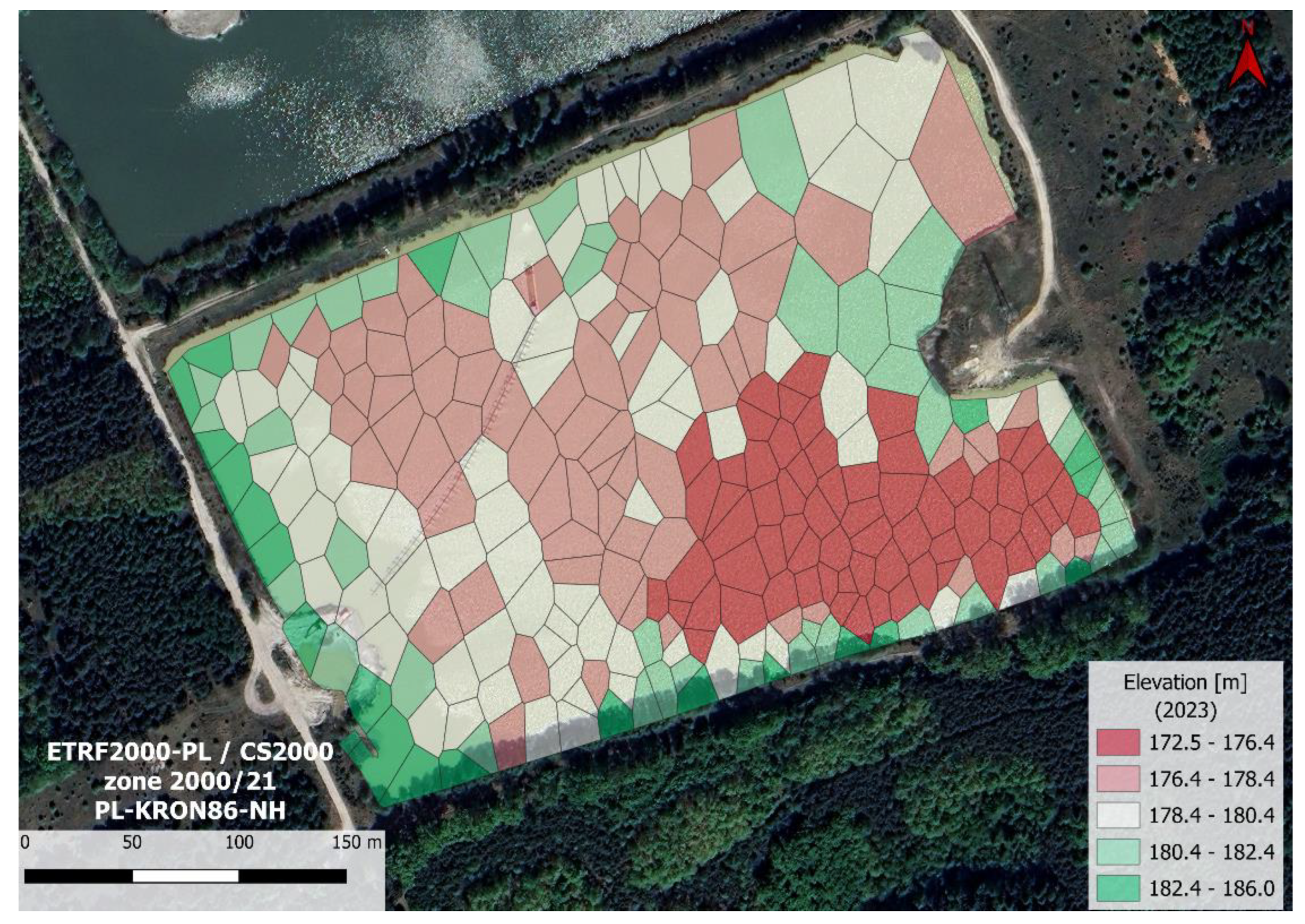
Figure 12.
Output layer “polygons – year 2” with applied styles.
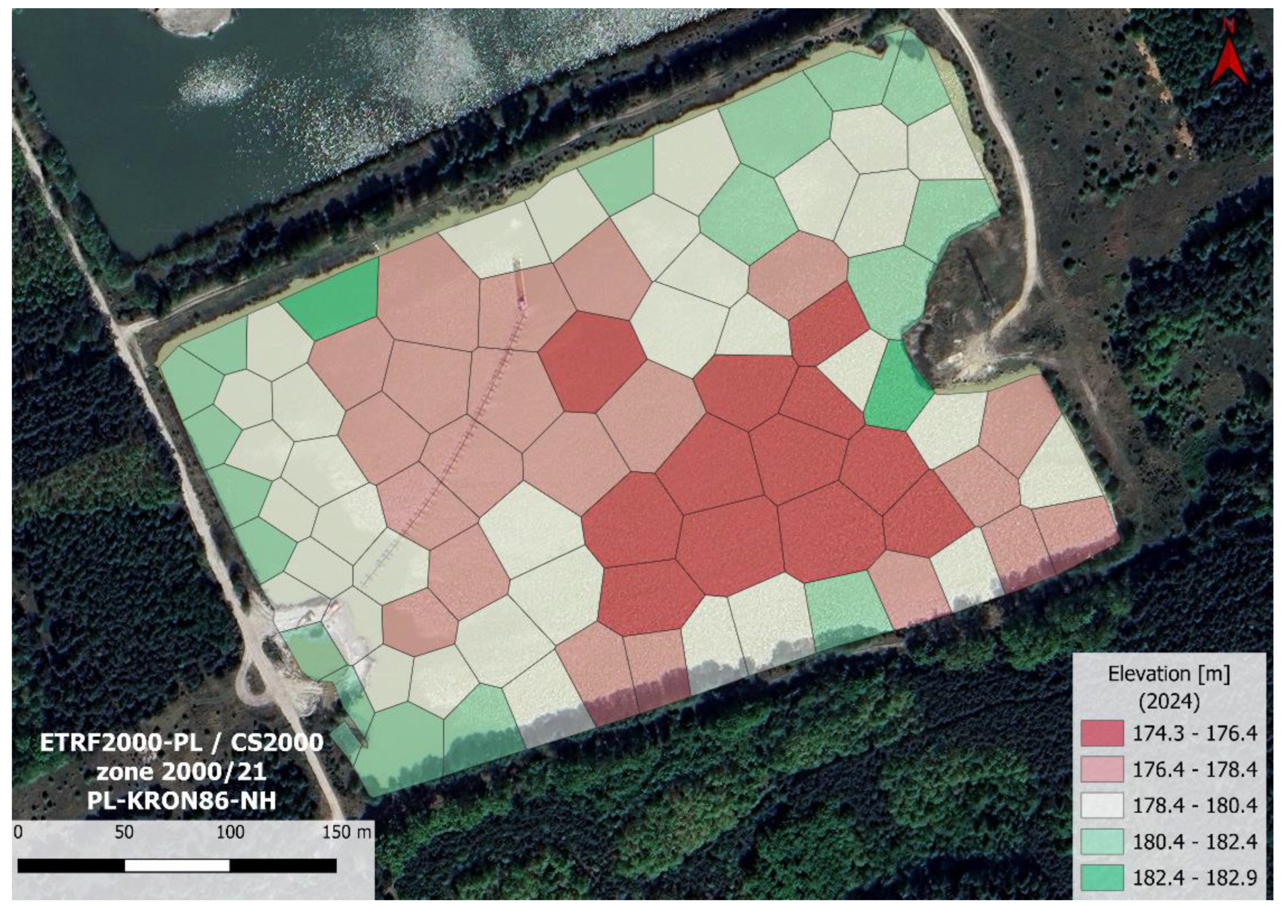
Figure 13.
Output layer “intersection of polygons and polygons 2” with applied styles.
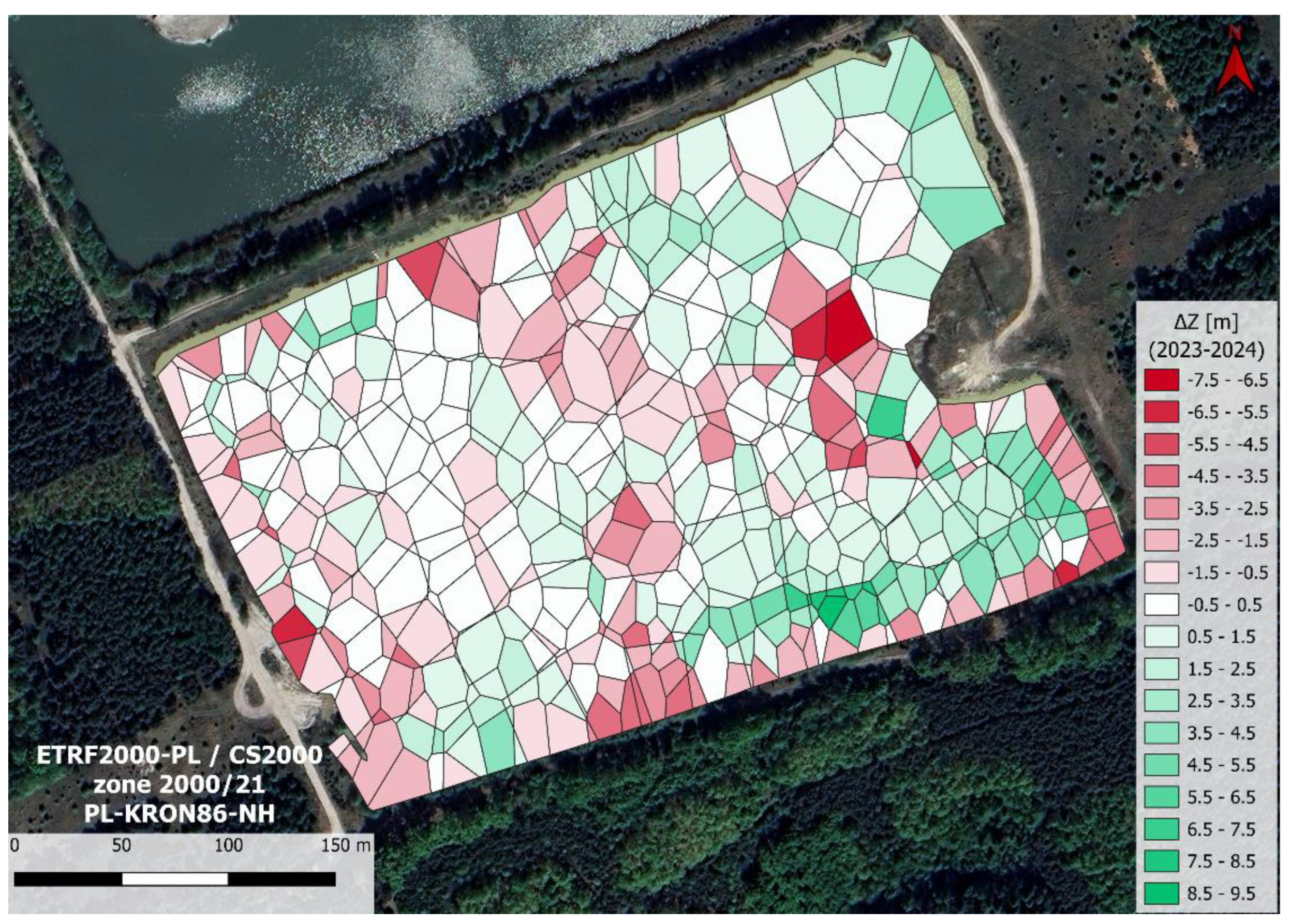

Table 1.
Requirements and parameters of “Create Voronoi polygons” procedure.
| Input | Parameters | Output |
|---|---|---|
| Vector layer: point | Buffer region | Vector layer: polygon |
| Tolerance | ||
| Copy attributes from input features |
Table 2.
Requirements and parameters of “Intersection” procedure.
| Input | Parameters | Output |
|---|---|---|
| Any vector layer (to overlay) | Input fields | The same dimension vector layer as overlayed layer |
| At least the same dimension vector layer (overlaying) | Overlay fields |
Table 3.
Requirements and parameters of “Calculate volumes” procedure.
| Input | Parameters | Formula | Output |
| Any vector layer | Field name | Expression for calculations | INPUT with modified attribute table |
| Field type Field length Field precision |
Disclaimer/Publisher’s Note: The statements, opinions and data contained in all publications are solely those of the individual author(s) and contributor(s) and not of MDPI and/or the editor(s). MDPI and/or the editor(s) disclaim responsibility for any injury to people or property resulting from any ideas, methods, instructions or products referred to in the content. |
© 2025 by the authors. Licensee MDPI, Basel, Switzerland. This article is an open access article distributed under the terms and conditions of the Creative Commons Attribution (CC BY) license (https://creativecommons.org/licenses/by/4.0/).
Copyright: This open access article is published under a Creative Commons CC BY 4.0 license, which permit the free download, distribution, and reuse, provided that the author and preprint are cited in any reuse.


