
Submitted:
07 May 2025
Posted:
08 May 2025
You are already at the latest version
Abstract
Accurate and detailed spatial data on wind energy infrastructure is essential for renewable energy planning, grid integration, and system analysis. However, publicly available datasets often suffer from limited spatial accuracy, missing attributes, and inconsistent metadata. To address these challenges, this study presents a harmonized and spatially refined dataset of wind turbines in South Africa, combining OpenStreetMap (OSM) data with high-resolution satellite imagery, deep learning-based coordinate correction, and manual curation. The dataset includes 1,487 turbines across 42 wind farms, representing over 3.9 GW of installed capacity as of 2025. The Geo-Coordinates were validated and corrected using a RetinaNet-based object detection model applied to both Google and Bing satellite imagery. Instead of relying solely on spatial precision, the curation process emphasized attribute completeness and consistency. Through systematic verification and cross-referencing with multiple public sources, the final dataset achieves a high level of attribute completeness and internal consistency across all turbines, including turbine type, rated capacity, and commissioning year. The resulting dataset is the most accurate and comprehensive publicly available dataset on wind turbines in South Africa to date. It provides a robust foundation for spatial analysis, energy modeling, and policy assessment related to wind energy development. The dataset is publicly available for download and can be explored interactively online.
Keywords:
wind turbine location
; renewable energy
; deep learning
; geo-coordinate correction
; OpenStreetMap
1. Introduction
Wind energy is one of the fastest-growing renewable energy sources worldwide. In 2023, wind energy recorded its highest ever growth: in a single year, more than 100 GW of new onshore capacity and over 11 GW of offshore wind capacity were added globally. Total installed capacity worldwide exceeded the symbolic milestone of 1 TW for the first time and is expected to reach 2 TW before the end of this decade if current growth trends continue [3]. In addition, the International Energy Agency (IEA) forecasts scenarios in which wind energy could meet more than 20% of global electricity demand by 2030, provided that ambitious climate protection measures are implemented [4]. The transition to renewable energy sources presents major challenges. Accurate mapping and monitoring of wind turbine locations and meta-information on the turbine characteristics (e. g. turbine types, nominal power, hub height, or rotor diameter) are critical for effective integration into electricity grids and sustainable infrastructure planning.
Despite its growing global importance, detailed and spatially accurate datasets of wind turbine infrastructure remain scarce in many regions of the world. Existing global datasets often focus on aggregated capacities or rough location data, lacking precision for localized planning and operational decision-making. Recent research efforts address these limitations through advanced remote sensing and machine learning approaches. For instance, global offshore wind turbine locations were mapped using Sentinel-1 radar images [5,6], while segmentation methods utilizing high-resolution aerial images [7,8] and Sentinel-2 RGB imagery [9,10] improved the detection accuracy of onshore wind turbines. Moreover, the integration of multimodal data sources [11,12], further enhances detection accuracy and completeness. Even approaches to enable global detection are being researched [13,14].
In the specific context of South Africa, the national Renewable Energy Independent Power Producer Procurement Programme (REIPPPP) plays a central role in realizing the country’s long-term energy infrastructure goals. Launched in 2011 by the Department of Mineral Resources and Energy in cooperation with National Treasury and the Development Bank of Southern Africa, the REIPPPP was designed to facilitate private sector investment into grid-connected renewable energy generation through competitive bidding. The programme has since led to the procurement of more than 6.3 GW of renewable capacity, including wind, solar photovoltaic (PV), and other sources [15]. As part of this programme, the Independent Power Producers (IPP) Projects Database is maintained by the IPP Office and provides a structured overview of utility-scale renewable energy projects, including wind farms. The database includes information such as project names, capacities, locations, and commissioning dates. However, it does not contain detailed geospatial information on individual turbines and typically excludes smaller or non-utility-scale developments. At the same time, it does not provide any technical information such as turbine types, hub height, or rotor diameter [16]. Recent regulatory changes have further expanded the landscape of wind energy development in South Africa. In particular, the lifting of the 100 MW licensing cap for private generation in January 2023 has enabled the construction of wind farms outside the REIPPPP framework [17].
To overcome these data limitations, this article builds upon the methodologies initially presented in the conference paper by Kleebauer et al. (2024) entitled "Enhancing Wind Turbine Location Accuracy: A Deep Learning-Based Object Regression Approach for Validating Wind Turbine Geo-Coordinates" [18]. Here, the original methods are further developed, combining OSM data, DL-based object detection with RetinaNet, high-resolution satellite imagery from Google and Bing, and manual attribute enrichment, to produce a comprehensive, spatially precise dataset of wind turbines in South Africa. This multi-step pipeline ensures robust validation and enrichment, significantly enhancing data quality and applicability for detailed infrastructure planning and energy modelling. Structured as following, this study introduces a multi-step data processing pipeline that combines open data sources, deep learning-based coordinate correction, and manual validation.
As illustrated in Figure 1, the construction of the dataset follows a multi-stage workflow. First, training data is processed using the German Core Energy Market Data Register (ger: Marktstammdatenregister - MaStR) and high resolution areal imagery. A RetinaNet-based deep learning model is trained and fine-tuned using labeled MaStR data and filtered samples to detect turbines in satellite imagery. Preparing the South African wind turbine dataset starts with downloading, extracting and filtering the raw wind turbine data from OSM. High-resolution satellite imagery from both Bing Maps and Google Satellite is then integrated to provide visual context for turbine locations. The previous trained model is applied to correct the spatial positions of turbines, improving the coordination accuracy. Subsequently, a manual attribute enrichment step ensures the inclusion of key turbine information such as name, turbine type, turbine capacity and total wind farm capacities. A capacity analysis and a spatial analysis are then carried out for further description and evaluation. This leads to the final high-quality, geo-referenced data set of wind turbines in South Africa.
The work was carried out as part of the "Long-Term Joint EU-AU Research and Innovation Partnership on Renewable Energy (LEAP-RE) Program" in the project “Development and Demonstration of a Sustainable Open Access AU-EU Ecosystem for Energy System Modelling (OASES)”. As part of the project, a comprehensive open source strategy was developed to ensure good open source access to project results, enabling users worldwide to carry out renewable energy analyses with minimal barriers. This ecosystem ensures transparency and supports the wider adoption of open-source tools for energy planning and analysis. The model chain developed in OASES includes renewable energy system detection [19], high-resolution time series generation [20], and energy system modelling with integration into IRENA FlexTool [21].
2. Materials
2.1. OpenStreetMap
OSM is a collaborative, open-access mapping platform that provides geospatial data contributed and maintained by a global community of volunteers [22]. Established in 2004, OSM has become a leading source of freely available geographic information, covering diverse features such as roads, buildings, land use, and energy infrastructure. Its community-driven model ensures that the data is continuously updated and enriched, offering a valuable resource for research, spatial planning and analysis. For renewable energy studies, OSM often serves as an initial source for identifying the location and distribution of wind farms and other energy infrastructure. While OSM data provides extensive coverage, it frequently lacks consistent accuracy in spatial precision and technical detail. This is particularly evident for features such as wind turbine coordinates and capacity specifications, which may be missing or imprecise [23,24]. To address these limitations, this study validates and refines the locational data using complementary methodologies, such as high-resolution satellite imagery analysis and DL-based object detection approaches. To enable a comprehensive and regionally consistent extraction of the energy-related infrastructure, the complete OSM file for South Africa was downloaded from the Geofabrik [25]. Geofabrik offers daily updated and freely accessible OSM extracts for all regions worldwide. The file for South Africa, was used as the base dataset to ensure that no relevant entries were omitted due to incomplete or outdated online queries.
2.2. Google Satellite Data and Bing Image Data
Google Satellite Data and Bing Image Data provide high-resolution satellite imagery that is widely utilized for spatial analysis across various disciplines. Google Satellite imagery is accessible through platforms such as Google Earth Engine [26] or Google Maps [27], while Bing imagery is accessed through the Bing Maps API [28]. Both offer detailed views of the Earth’s surface, capturing features such as buildings, roads, and natural landscapes. For accurate validation or correction of existing geo-datasets of renewable energy sources, Google Satellite and Bing Image Data can be used as important resources for identifying and validating infrastructure locations, including wind farms and individual turbines. These datasets provide high-resolution imagery with true-color (red-green-blue) channels that provide realistic visual representations of surface features. This color channel information facilitates the identification and distinction of objects and their properties. In addition, the two satellite image data sets complement each other by providing additional perspectives and different dates of acquisition, which is useful for validating results and improving coverage in areas where one source may have better resolution or more recent data. By integrating Google and Bing satellite data with deep learning and remote sensing techniques, the accuracy, scalability, and reliability of spatial data analysis are significantly improved, providing a comprehensive and multiply-verified dataset for renewable energy infrastructure analysis. They were used for the application and coordinate correction of wind turbine locations in South Africa. In contrast, the training of the DL model was based on turbine coordinates from the German Core Energy Market Data Register (German: Marktstammdatenregister, MaStR) and high-resolution Digital Orthophotos (DOP).
2.3. Core Energy Market Data Register
The MaStR, administered by the Federal Network Agency for the German electricity and gas market, serves as a comprehensive database for energy market. Commencing operations in 2019, the register undergoes daily updates and encompasses detailed information on entities and facilities within the grid-bound energy supply market [29]. Alongside registered electricity generation units, the register also includes extensive listings of large-scale consumers. On the producer side, the MaStR provides location information, performance values, and specific plant characteristics for various energy sources, such as wind turbines, PV systems, biomass plants, hydro power plants, and conventional plants. The register offers a wealth of information specifically tailored to wind turbines like registration date, commissioning date, rated power, remote controllability, current operating status, manufacturer, type designation, hub height, and rotor diameter. While freely accessible address data is generally available for all facilities at zip code level, for most wind turbines there are even detailed coordinates for determining the location of the individual turbines. As of November 21, 2023, out of the 32,788 listed turbines in operation, 31,892 include coordinate information.
2.4. Digital Orthophotos
The DOP of Germany, as documented by the Federal Agency for Cartography and Geodesy, constitute georeferenced and differentially rectified aerial imagery, sourced from the surveying administrations of Germany’s federal states [30]. These images faithfully represent the Earth’s surface, within the confines of the Federal Republic of Germany, employing a ground resolution of 0.2 m for the purposes of this investigation. The dataset encompasses both color images in the RGB spectrum. The images maintain a positional accuracy of ±0.4 m standard deviation. The entire dataset covers Germany and is presented in tiles measuring 1,000 × 1,000 m, equivalent to 5,000 × 5,000 pixels each. Each tile is accompanied by a file containing meta-information, notably the timestamp indicating when the respective image was captured. The image data is updated cyclically, usually available every 3 years in site-specific overflight intervals.
3. Methods
3.1. Training data preprocessing
The preparation of training data comprises multiple steps. Initially, all wind turbines registered in Germanys MaStR are loaded. A pre-filtering process is then applied, focusing exclusively on wind turbines with operational status labeled as "in operation". Additionally, the turbines must be categorized as "onshore", and only systems with available coordinates are considered. Finally, turbines situated outside the German federal border are excluded under the assumption that their location data is inaccurate. Existing coordinates of the turbines are provided with a static buffer of 30 m radius in order to obtain an area-like imprint of the point coordinates. These are required for the subsequent regressive localization method.
To generate training image data, the wind turbine location data is combined with DOPs. To align with the requirements of RetinaNet, DOP tiles, each measuring 5,000 × 5,000 pixels, are further divided into 1,000 × 1,000 pixel tiles. For training, the cut edges are statically selected to generate 15 tiles from each original tile, as illustrated on the left side in Figure 2. This approach ensures that wind turbines are not consistently positioned at the center of the image sections. Conversely, for application images, the wind turbine location is designated as the centroid of the image. Approximately 12,000 images are produced, each containing at least one wind turbine.
This dataset is utilized for the initial training. To ensure that highly suitable image data is used in the subsequent second training session, automatically generated examples are subjected to manual review. This process identifies and removes instances with incorrect coordinates stored in MaStR, imprecise coordinates, and image scenes with insufficient resolution. The re-selection leads to the reduction of a further 5,000 unsuitable images, yielding a dataset of 7,000 images for the second training. The primary emphasis is on the precise localization of wind turbines, ensuring that the center of the regression boxes accurately represents the tower’s exact ground location. As illustrated in Figure 3, several samples are depicted to exemplify their suitability. The training is divided into two parts. First, all 12,000 samples automatically derived from the data preprocessing are used, whereas in the second training, the number of samples is reduced to 7,000 highly suitable samples by manual filtering. All other parameters remained the same for both the first and second training: 100 epochs, 100 steps, 80 % training and 10 % independent validation, and 10 % test data set.
3.2. Deep Learning Approach
Several object detection frameworks were considered for the coordinate correction task, including Faster R-CNN, YOLOv3, and RetinaNet. RetinaNet was selected due to its balance between high detection accuracy and computational efficiency, particularly in scenarios with class imbalance, such as the detection of sparsely distributed wind turbines in large aerial images. The Focal Loss mechanism employed by RetinaNet has proven to significantly improve detection performance for rare objects compared to conventional cross-entropy loss in other architectures [31]. In addition, RetinaNet achieves competitive results in common object detection benchmarks (e.g., COCO dataset), while offering simpler training requirements compared to two-stage detectors like Faster R-CNN. RetinaNet is an object detection model that combines classification and regression within a unified architecture. It integrates several well-established DL techniques to enable high-precision object localization and classification. A key component is the Residual Network (ResNet) architecture, a variant of Convolutional Neural Networks (CNNs), which utilizes skip connections between layers to facilitate residual learning and improve gradient flow in deep networks [31,32]. To handle multi-scale object detection, a Feature Pyramid Network (FPN) is employed on top of the backbone. The FPN uses a top-down architecture with lateral connections to generate semantically rich feature maps at multiple scales [33]. This allows the network to detect objects of varying sizes effectively. The classification subnetwork is trained using the Focal Loss, which was specifically developed to address the problem of class imbalance between foreground and background objects in dense detection tasks [31]. Unlike the standard cross-entropy loss, Focal Loss introduces a modulation factor to down-weight easy examples and focus training on hard negatives. The formula for Focal Loss is:
where is the model’s estimated probability for the true class, is the weighting factor for class imbalance (), and is the focusing parameter (). This formulation ensures that well-classified examples receive less weight, allowing the model to focus on misclassified or more difficult samples. The regression subnetwork is responsible for predicting bounding boxes around detected objects. It uses the Smooth L1 Loss function, which combines the benefits of L1 and L2 losses and is less sensitive to outliers. This loss was originally introduced in the Fast Region-based Convolutional Network Network (Fast R-CNN) architecture [34]. The regression loss is computed for the predicted bounding box tuple and the ground truth box as:
The Smooth L1 function itself is defined as:
The smoothing parameter was set to its commonly used default value of 3.0. This loss formulation enables stable training and effective bounding box regression even in the presence of noisy labels. RetinaNet outputs bounding boxes with predefined aspect ratios of 1:2, 1:1, and 2:1 [31].
Model performance is evaluated using the Average Precision (AP) metric, following the Common Objects in Context (COCO) detection benchmark, where predictions are considered correct if their Intersection over Union (IoU) with ground truth is above 50%. To calculate AP, two basic metrics are first needed, Precision and Recall. Precision measures the proportion of correctly identified objects (true positives) among all identified objects (true positives and false positives):
Recall quantifies the proportion of correctly identified objects among all actual objects (true positives and false negatives):
The AP is then obtained by calculating the area under the precision-recall curve:
The implementation is based on the open-source keras-retinanet package [35], which was developed specifically for RetinaNet applications.
3.3. South Africa Wind Turbine Pre-Dataset
Initially, OSM is used to derive the dataset of all wind turbines in South Africa, based on downloading a complete set of OSM data for South Africa via the Geofabrik download service [25], followed by filtering using the “esy-osmfilter” tool [36]. The filtering is done to extract relevant energy infrastructure, with a focus on renewable energy facilities such as wind turbines and PV systems. The filtering process involves using predefined filter criteria to ensure that only the required energy infrastructure elements are selected:
- Prefilter: The `prefilter` is used to identify nodes, ways, and relations tagged with attributes like `"power": ["generator", "plant", "solar", "photovoltaic"]` to capture all relevant renewable energy installations.
- Blackfilter: A `blackfilter` is applied to exclude certain types of infrastructure that are not of interest, such as those associated with fossil fuels or hydro-based generation. Examples include `("generator:source", "gas")`, `("generator:method", "combustion")`, and `("generator:source", "coal")`.
- Whitefilter: A `whitefilter` is also used to ensure that elements explicitly tagged with `("power", "generator")` are retained in the dataset.
This process provides a refined dataset that filters out non-relevant elements and focuses on renewable energy facilities, improving the quality and relevance of the geospatial analysis.
3.4. South Africa’s wind turbines coordinate correction
The model is applied to high-resolution satellite images provided by Google Satellite as well as Bing image. The initial coordinates for the images are taken from the OSM dataset, with each wind turbine’s OSM coordinate serving as the centroid for image extraction. The prepared tiles for analysis are each 640 × 640 pixels with a resolution of 20 × 20 cm. This allows for a focused examination of each turbine location and subsequent adjustment based on the model’s predictions. The restriction on the size of the images depends on the permitted options of the services. To generate the coordinates of the final data set, the resulting coordinates with highest confidence score are adopted. If the confidence score falls below the threshold of 0.2, an additional manual verification is applied.
3.5. Additional attribute Enrichment
The additional step of attribute enrichment was to manually add detailed information about the wind farms, including wind farm names, turbine capacities, total farm capacities, turbine types and commissioning years. These attributes were collected through manual enrichment, which was crucial to ensure the accuracy and completeness of the dataset. For this purpose, the operators’ websites or publications about the construction of the farms were searched for where possible and used our information enrichment. In addition to the technical attributes, we assigned spatial information by intersecting each wind farm site with administrative boundaries using the Global Administrative Areas (GADM) dataset [37]. For each site, the corresponding country and first and second level administrative units were identified and added to the dataset. For this purpose, the coordinates of each wind turbine are spatially allocated to corresponding administrative polygons. If a wind farm location was outside a defined polygon due to geometric inaccuracies, it was mapped to the nearest administrative unit to ensure completeness. This referencing simplifies regional analysis and the combination with other datasets.
4. Results
Initially, we briefly present the results from model training, the data extracted and processed from OSM, followed by the results of the location correction. Finally, we present the results of the additional attribute enrichment.
4.1. Performance and Results of Deep Learning Training
This section presents the results of the DL training, including the loss functions and the accuracy achieved. These results provide insight into the robustness and performance of the applied RetinaNet approach. As Training Progress Summary, the progression of the two losses from the classification and regression networks, as well as the AP, were validated to determine the networks’ performance, as displayed in Figure 4.
Shown in blue are the results of the first training session, in which all training data was used, and in red the second training session, in which the training data was used after filtering. A consistent upward trend can be observed in the AP. Finally, the AP is 85% for the first training and 96% for the second training with manually post-filtered samples. In addition, the following Figure 5 shows the losses during training phase.
Both the regression loss used to localize the objects and the Smooth L1 loss used for classification decrease significantly and almost evenly in both training runs. The total loss represents the cumulative sum of the individual losses. The training is terminated by early stopping after 17 epochs in each case, indicating no further progress in training. Overall, the loss and AP’s curves clearly show the strong generalization of the network based on the training examples. Incorrect recognition are shown in Figure 6.
This includes a construction site, a biogas plant and two churches. Secondly, some of the poorly represented turbines are not recognized by the network. This applies to different backgrounds, so that turbines in open fields, in the forest and also in the settlement are not recognized. However, they are also difficult to identify during a visual inspection. Examples of correctly recognized wind turbines, conversely, are shown in Figure 7. In addition to turbines with good resolution, poorly resolved turbines can also be identified in the images. All images show that the regression locates the towers of the turbines exactly in the centers of the bounding boxes. In other words, the centers of the regression boxes can be interpreted as exact coordinates of the wind turbines.
4.2. OSM Data Extraction
The initial data set for South Africas wind turbines, extracted from OSM, contained a total of 1,546 point features. After a manual review and refinement process, this number was reduced to 1,487 verified wind turbines. Point features with the tags generator and diesel as well as solar were excluded and deleted. However, 55 turbines in the OSM data are not assigned to any wind farm. These are added manually. Among the wind farms, Longyuan Mulilo de Aar 2 North has the highest number of turbines with 96 individual units, while the smallest wind farm, Buffeljags Abalone Farm, consists of only two turbines. For all turbines without an associated wind farm, a manual assignment to the respective farms was carried out to ensure the completeness of the data. A capacity is given for 351 of the 1,487 turbines, while no capacity data is available for 1,144 turbines. This ensures that all wind turbines are assigned to a wind farm and capacity information if possible.
4.3. Coordinate Correction
The accuracy of the neural network’s predictions heavily depends on the domain-specific characteristics of the training and application datasets. To analyze this effect, we compare the confidence scores of the predictions for onshore wind turbines in South Africa. Table 1 presents the results of the coordinate correction process using both Bing and Google satellite imagery.
The Table summarizes results for 1,487 wind turbines, showing that the overall distribution of confidence scores differs considerably between Bing and Google imagery. While only a small fraction of detections reaches confidence scores above 0.8 (0.2% for Bing and 3.0% for Google), the majority falls below 0.5, indicating potential challenges in image consistency or domain transfer. Despite this, visual inspection confirms the accurate detection of turbines in both datasets, as illustrated in Figure 8 and Figure 9.
A total of 90 turbines (6.05%) on the Bing images and 43 turbines (2.89%) on the Google images are not detected and thus fall into the null category. The analysis shows that 36 of the non-detected South African wind turbines are matched by Bing and Google. All these overlaps are exclusively located within four specific farms: San Kraal Wind Farm, Phezukomoya, Cookhouse Wind Farm, and Wolf Wind Farm. The visual inspection of the zero category shows that there are often construction sites for wind turbines at the locations, which means that some of the images are not up-to-date enough to show the existing wind turbine. In addition to the accuracy of the detection, the accuracy of the regression is examined in the following. Table 2 summarizes the distances between pre-dataset coordinates and regression analysis.
The Table 2 presents the distribution of coordinate deviations for wind turbines in South Africa, comparing results derived from Bing and Google Maps. The deviations are categorized into six distance intervals: <5 m, 5–10 m, 10–15 m, 15–20 m, 20–25 m, and >25 m. A significant portion (64.3%) of the Google-based coordinates fall within 10 m of the reference, whereas only 29.4% of the Bing-based coordinates achieve this accuracy. The largest deviations (>25 m) occur in 16.6% of Bing and 12.9% of Google. To provide a visual summary of the distribution of location errors, a histogram of the distance deviations was created, as indicated in Figure 10. It shows the proportion of turbines falling within specific distance ranges for both Bing and Google images.
4.4. Wind turbine dataset
An overview of the existing wind farms in South Africa is provided below. The summarizing Table 3 combines spatial information with key technical attributes for each wind turbine. It includes both operational and under-construction sites and was cross-checked and harmonized based on multiple publicly available sources. Listed are commissioning years, the number of turbines, the total installed capacity in MW, the rated capacity per turbine in MW and the type of turbine installed in each wind farm.
Two wind farms, Phezukomoya and San Kraal, are still under construction. In these cases, not all turbines have yet been built or identified, which explains deviations from the detailed point-based turbine dataset. A more detailed graphical evaluation is summarized in Figure 11. Boxplots illustrate three key parameters from left to right: the number of turbines per wind farm, the total installed capacity, and the specific capacity per turbine.
The number of turbines varies significantly, ranging from small farms with only 2 to 4 turbines to large-scale farms hosting up to 96 turbines. However, the majority of wind farms contain between around 15 and under 50 turbines. On average, there are 37 turbines within a farm. The total installed capacity per wind farm ranges from as little as 0.1 MW to 147 MW. The majority of projects lie within the interquartile range of 35 to 140 MW, the median is 100 MW. The nominal capacity per turbine spans a wide range, from small-scale units with 25 kW to modern high-capacity turbines rated at 4.5 MW. Most turbines, however, fall within the interquartile range of 2.3 to 3.1 MW, with mean capacity of a turbine is 2.5 MW, typical for recent onshore turbine installations.
Figure 12 shows the development of wind power capacity in South Africa over time, starting with the first installations in 2008 through to 2025. To illustrate the growth trend in recent years, the left panel shows the annual installed capacity between 2008 and 2025 based on the commissioning years of the individual wind farms. At least three different phases of capacity growth can be observed: an initial phase with isolated installations between 2008 and 2012, a first strong expansion phase from 2014 to 2021 with significant annual growth and a second expansion phase since 2022. The largest annual increases were in 2016 with around 580 MW and in 2021 with almost 570 MW of newly installed capacity. The right panel shows the cumulative installed capacity over the same period. By 2025, the total installed capacity will reach over 3.9 MW.
Figure 13 shows the total installed capacity per wind farm in descending order, distributed across 42 different wind farms with capacities ranging from 147 MW to 0.1 MW. The bar lengths provide a quick indication of the relative capacity of the individual wind farms. This ranking makes it easier to identify the wind farms in South Africa with the highest rated capacity. The largest farms - such as Roggeveld, Karusa, Nxuba or Soetwater - reach around 140-150 MW. The smallest wind farms such as Coega, Buffeljags Abalone Farm and Silo Distict’s Sustainable Design have significantly lower total capacities of less than 2 MW.
Alongside the total installed capacity, the Figure 14 shows the number of wind turbines installed in the individual wind farms in descending order. The order provides a quick overview of the locations with a particularly high amount of turbines. Longyuan Mulilo De Aar 2 North stands out with 96 turbines, while Longyuan Mulilo De Aar Maanhaarberg with 67 turbines and Cookhouse Wind Farm with 66 turbines are the next largest farms. Coega Wind Farm has only two turbines. In combination with the capacity data, this also gives an indication of the average turbine size in each wind farm.
The Figure 15 shows the nominal capacity per wind turbine at each wind farm. This overview can be used to determine which sites mainly use smaller turbines and which rely on turbines with a higher rated capacity. The frequent use of turbines with a capacity of 2.3 MW (here with Siemens SWT-2.3 turbines) in the Jeffreys Bay Wind Farm, Kangnas Wind Farm, Khobab Wind Farm, Loeriesfontein 2, Noupoort Mainstream, and Perdekraal East Wind Farm is particularly evident. However, turbines with a capacity of 3 MW are also widely used in Dassieklip, Chaba Wind Farm, Copperton Wind Farm, Gouda Wind Facility, Red Cap - Gibson Bay, and Van Stadens Wind Farm. The lower end of the scale includes turbines with relatively small capacities, such as those at Buffeljags Abalone Farm or the vertical axis turbines in the Silo District. Higher bars correspond to larger capacity turbines, such as the Vestas V136 and V162 models with capacities with up to 5 MW.
The following section of the results focuses on the spatial distribution of wind turbines in South Africa. The installed wind power capacity is concentrated in just three of the country’s nine provinces, Northern Cape, Eastern Cape, and Western Cape. Table 4 provides a summary of wind energy infrastructure at the provincial level.
The majority of capacity is located in the Northern Cape and Eastern Cape, which together host 32 wind farms and 1,231 turbines. The Western Cape follows with 10 wind farms. Together, the Eastern Cape and the Northern Cape account for 1,571 MW and 1,670 MW of installed capacity, respectively. The Western Cape contributes 575 MW, bringing the total installed capacity in these three provinces to more than 3,800 MW. The Roggeveld Wind Farm represents a special case, as it spans across two provinces. Since the majority of its 42 turbines are located in the Northern Cape and only five fall within the Western Cape, the entire wind farm is attributed to the Northern Cape for consistency in the provincial analysis.
Figure 16 illustrates the spatial distribution of all 42 existing wind farms in South Africa. It clearly shows that the facilities are exclusively located in the southwestern provinces, particularly in the Northern Cape, Eastern Cape, and Western Cape. To supplement the analysis at provincial level, a more detailed spatial aggregation was carried out at district municipality level. This approach enables a finer resolution of the spatial distribution and highlights the differences within the provinces in the expansion of wind energy. Figure 17 shows the total installed capacity on the one hand and the number of wind turbines per municipality on the other. The results show a very uneven distribution, with a limited number of municipalities hosting the majority of turbines and installed capacity. In contrast, many regions are still completely undeveloped, indicating a significant spatial concentration of wind energy infrastructure.
5. Discussion
This study presents a comprehensive and spatially validated dataset of wind power infrastructure in South Africa. With 1,487 turbines across 42 wind farms and a total installed capacity exceeding 3.9 GW, the dataset offers both spatial and technical detail. Most turbines are concentrated in the Northern Cape, Eastern Cape, and Western Cape provinces, reflecting the regional clustering of wind development in the country. In addition to the spatial information, the dataset includes harmonized metadata such as commissioning year, turbine type, wind farm capacity, and per-turbine capacity. These attributes were manually collected and cross-checked from various sources.
Although labor-intensive, this enrichment process significantly increases the usability and reliability of the dataset—enabling advanced applications in energy system modelling, infrastructure planning, and policy design. However, manually collecting turbine-specific information also revealed common challenges regarding the availability and quality of public data. The information on operators’ websites was often unstructured, inconsistently formatted, or partially incomplete. In several cases, additional sources such as press releases, freely accessible news articles, and energy-related databases were consulted. While these secondary sources were useful for cross-checking, they sometimes contained unverifiable or contradictory data, highlighting the limitations of public reporting on renewable energy infrastructure. These challenges underline the crucial role of manual processing within the overall pipeline, which, despite advances in automation, remains indispensable for ensuring technical completeness and high data quality.
While most of the data processing, including the localization of the turbines for coordinate correction using DL methods, was automated, manual steps were essential to ensure the technical completeness and reliability of the dataset. In particular, turbine attributes such as turbine type, capacity and year of commissioning were manually enriched by comparing several publicly available sources (e.g. operator website, project reports, press releases). This manual effort was necessary because the detailed technical metadata in open data sets such as OSM or national databases is almost completely missing, incomplete or inconsistent. If the pipeline were transferred to other countries or regions, a similar manual enrichment step would probably be required due to the heterogeneous availability of data and the different reporting standards worldwide. Automated extraction of attributes from semi-structured text sources (e.g. using natural language processing methods) could be investigated as a future extension to partially automate this step. However, full automation is currently only possible to a limited extent due to the lack of standardized and structured publication of turbine metadata. Furthermore, regular updates of the dataset (e.g. every 1-2 years) would require re-verification of new wind farm projects and updating of technical attributes, meaning that some level of manual verification and enrichment will still be essential to maintain data quality. Nevertheless, further improvements, such as the integration of automated web scraping techniques combined with manual quality checks, could significantly reduce the manual workload while ensuring high standards of data accuracy.
The dataset was systematically checked against several external sources to ensure its completeness. A comparison with the official database of the South African IPP Database [16] confirms that all 34 large wind farms currently in operation are included in this dataset. In addition, two projects under construction and several smaller wind farms that are not listed in the official database have been included. The dataset thus shows that it not only covers large infrastructure, but also takes into account smaller and newly emerging projects. The dataset therefore provides a more comprehensive picture of the national wind energy landscape than existing centralized sources.
The coordinate correction process based on RetinaNet was trained on German aerial imagery and applied to South African wind turbine locations using both Bing and Google satellite data. The application resulted in a notable drop in confidence scores, which can be attributed to the domain shift between training and application imagery—a typical challenge in DL when transferring models across data sources. Despite this, the visual and statistical evaluation confirms a high localization accuracy. More than 60% of Google-based predictions and 29% of Bing-based predictions fall within a 10 m range from the reference coordinates. The model’s ability to correctly identify turbine locations across different landscapes and image types confirms its practical value as a scalable validation tool.
However, some aspects of the detection and correction process could be improved in future applications. First, the exclusive use of a RetinaNet architecture could limit performance in more complex or visually diverse environments. Alternative approaches—such as modern transformer-based detection models—could offer greater robustness and accuracy, particularly under conditions of visual ambiguity or clutter. Second, the image data itself could be further diversified. The current approach is limited to single time frames from Bing and Google images, which may not capture seasonal variations or recent changes in infrastructure. The use of time series images or higher-resolution commercial data could improve model generalization and enable the detection of newer or smaller installations.
From a methodological perspective, the study highlights the importance of combining open spatial data, deep learning, and manual curation to overcome the usual limitations of public datasets. OSM offers broad coverage but lacks standardization and, in some cases, location accuracy. The integration of DL fills this gap by refining the location data, while manual enrichment ensures the completeness and technical detail required for meaningful application. Together, these components form a transferable and reproducible workflow for the creation of high-quality renewable energy datasets in data-poor regions.
6. Conclusions
This study presents the most accurate, comprehensive, and up-to-date dataset on wind turbines and wind farms currently available for South Africa. By integrating publicly available OSM data, high-resolution satellite imagery, and advanced DL-based coordinate correction using RetinaNet, the spatial accuracy of turbine locations has been significantly improved. The dataset has been further enhanced through manual enrichment with important technical and temporal attributes such as wind farm names, turbine types, capacities, and commissioning years—information that is often missing or inconsistent in existing sources. Spatial metadata has been mapped to administrative boundaries from the GADM database, enabling regional analysis and integration with other relevant datasets.
This dataset thus provides accurate turbine coordinates, technical specifications, and harmonized metadata. It includes not only all large wind farms currently listed in the South African IPP project database, but also smaller and emerging wind farms that are not covered by official sources. The result is a high-quality, freely accessible dataset that provides a solid foundation for research, energy system modelling, infrastructure planning, and policy evaluation. It makes an important contribution to the open energy data landscape and provides a transferable methodology for creating similarly detailed datasets in other countries and for other renewable energy technologies. The dataset is freely available for download [1] and can be used interactively [2]. We strongly encourage its reuse and further development by the broader research and planning community.
Author Contributions
In the following paragraph, the individual contributions of the authors are briefly broken down with regard to the publication. The authors are abbreviated as follows: Maximilian Kleebauer (M.K.), Stefan Karamanski (S.K.), Doron Callies (D.C.), and Martin Braun (M.B.). Conceptualization, M.K., S.K.; methodology, M.K.; software, M.K.; validation, M.K., S.K.; formal analysis, M.K.; investigation, M.K.; resources, M.K.; curation, M.K., S.K.; writing—original draft preparation, M.K.; writing—review and editing, M.K., M.B., D.C., S.K.; visualization, M.K.; supervision, M.K.; project administration, M.K.; funding acquisition, M.K., D.C. All authors have read and agreed to the published version of the manuscript.
Data Availability Statement
The dataset processed during this study is available at DOI: 10.5281/zenodo.15221465
Acknowledgments
This work was done as part of the Long-Term Joint EU-AU Research and Innovation Partnership on Renewable Energy (LEAP-RE) Program. LEAP-RE has received funding from the European Union ’s Horizon 2020 Research and Innovation Program under Grant Agreement 963530. The Project "Development and Demonstration of a Sustainable Open Access AU-EU Ecosystem for Energy System Modelling" (OASES) within LEAP-RE is founded by the German Federal Ministry of Education and Research (03SF067) to University of Kassel and partly funded by the Council for Scientific and Industrial Research (CSIR) and the South African National Energy Development Institute (SANEDI). The authors would like to thank the editors and reviewers for their advice.
Conflicts of Interest
The authors declare no conflict of interest.
Abbreviations
The following abbreviations are used in this manuscript:
| AP | Average Precision |
| AU | African Union |
| CNN | Convolutional Neural Network |
| COCO | Common Objects in Context |
| DL | Deep Learning |
| DOP | Digital Orthophotos |
| EU | European Union |
| Fast R-CNN | Fast Region-based Convolutional Neural Network |
| FPN | Feature Pyramid Network |
| GADM | Global Administrative Areas |
| IoU | Intersection over Union |
| IPP | Independent Power Producers |
| IRENA | International Renewable Energy Agency |
| LEAP-RE | Long-Term Joint EU-AU Research and Innovation Partnership on Renewable Energy |
| MaStR | Marktstammdatenregister (Core Energy Market Data Register) |
| MDPI | Multidisciplinary Digital Publishing Institute |
| OASES | Open Access AU-EU Ecosystem for Energy System Modelling |
| OSM | OpenStreetMap |
| PV | Photovoltaic |
| QGIS | Quantum Geographic Information System |
| REIPPPP | Renewable Energy Independent Power Producer Procurement Programme |
| ResNet | Residual Network |
| RGB | Red, Green, Blue |
| Zenodo | Open-access repository for archiving research outputs |
References
- Kleebauer, M. Dataset according to "A Wind Turbines Dataset for South Africa: Open Street Map Data, Deep Learning Based Geo Coordinate Correction and Capacity Analysis", 2025. Accessed on April 28, 2025. [CrossRef]
- Kleebauer, M. South Africa Wind Turbine Dataset. Hosted on Google My Maps, 2025. Accessed on April 2025.
- Global Wind Energy Council. Global Wind Report 2024, 2024. Accessed on April 22, 2025.
- International Energy Agency (IEA). World Energy Outlook 2022. Available online: https://www.iea.org/reports/world-energy-outlook-2022 (accessed on 17 January 2025).
- Zhang, T.; Tian, B.; Sengupta, D.; Zhang, L.; Si, Y. Global offshore wind turbine dataset. Scientific Data 2021, 8, 191. [Google Scholar] [CrossRef] [PubMed]
- Hoeser, T.; Feuerstein, S.; Kuenzer, C. DeepOWT: A global offshore wind turbine data set derived with deep learning from Sentinel-1 data. Earth System Science Data 2022, 14, 4251–4270. [Google Scholar] [CrossRef]
- Han, M.; Wang, H.; Wang, G.; Liu, Y. Targets mask U-Net for wind turbines detection in remote sensing images. The International Archives of the Photogrammetry, Remote Sensing and Spatial Information Sciences 2018, 42, 475–480. [Google Scholar] [CrossRef]
- Darapaneni, N.; Jagannathan, A.; Natarajan, V.; Swaminathan, G.V.; Subramanian, S.; Paduri, A.R. Semantic Segmentation of Solar PV Panels and Wind Turbines in Satellite Images Using U-Net. In Proceedings of the 2020 IEEE 15th International Conference on Industrial and Information Systems (ICIIS). IEEE. 2020; 7–12. [Google Scholar]
- Mommert, M.; Scheibenreif, L.; Hanna, J.; Borth, D. Power plant classification from remote imaging with deep learning. In Proceedings of the 2021 IEEE International Geoscience and Remote Sensing Symposium IGARSS. IEEe. 2021; 6391–6394. [Google Scholar]
- He, T.; Hu, Y.; Li, F.; Chen, Y.; Zhang, M.; Zheng, Q.; Jin, Y.; Ren, H. Mapping land-and offshore-based wind turbines in China in 2023 with Sentinel-2 satellite data. Renewable and Sustainable Energy Reviews 2025, 214, 115566. [Google Scholar] [CrossRef]
- Mandroux, N.; Drouyer, S.; Grompone von Gioi, R. Multi-Date Wind Turbine Detection on Optical Satellite Images. ISPRS Annals of the Photogrammetry, Remote Sensing and Spatial Information Sciences 2022, 2, 383–390. [Google Scholar] [CrossRef]
- Yang, P.; Zou, Z.; Yang, W. Mapping Wind Turbine Distribution in Forest Areas of China Using Deep Learning Methods. Remote Sensing 2025, 17. [Google Scholar] [CrossRef]
- Robinson, C.; Ortiz, A.; Kim, A.; Dodhia, R.; Zolli, A.; Nagaraju, S.K.; Oakleaf, J.; Kiesecker, J.; Ferres, J.M.L. Global Renewables Watch: A Temporal Dataset of Solar and Wind Energy Derived from Satellite Imagery. arXiv preprint arXiv:2503.14860, 2025. [Google Scholar]
- Fei, Y.; Gao, Y.; Gu, H.; Sun, Y.; Tian, Y. YOLOv5_CDB: A Global Wind Turbine Detection Framework Integrating CBAM and DBSCAN. Remote Sensing 2025, 17, 1322. [Google Scholar] [CrossRef]
- Eberhard, A.; Naude, R. The South African renewable energy independent power producer procurement programme: A review and lessons learned. Journal of Energy in Southern Africa 2016, 27, 1–14. [Google Scholar] [CrossRef]
- Department of Electricity and Energy, Republic of South Africa. IPP Projects Database. Available online: https://www.ipp-projects.co.za/ProjectDatabase (accessed on 23 April 2025).
- Mashatile, P. Remarks by Deputy President Shipokosa Paulus Mashatile at the South Africa-Ireland Business Forum, 2023. Accessed on Mai 06, 2025.
- Kleebauer, M.; Braun, A.; Horst, D.; Pape, C. Enhancing wind turbine location accuracy: A deep learning-based object regression approach for validating wind turbine geo-coordinates. In Proceedings of the IGARSS 2024-2024 IEEE International Geoscience and Remote Sensing Symposium. IEEE. 2024. [Google Scholar]
- Kleebauer, M.; Marz, C.; Reudenbach, C.; Braun, M. Multi-Resolution Segmentation of Solar Photovoltaic Systems Using Deep Learning. Remote Sensing 2023, 15, 5687. [Google Scholar] [CrossRef]
- Botha, N.; Coleman, T.; Wessels, G.; Kleebauer, M.; Karamanski, S. Power generation time series for solar energy generation: Using ATlite in South Africa. Solar 2024, 4. [Google Scholar] [CrossRef]
- Niemi, A.; Bouchakour, S.; Ismail, B.; Bouchouicha, K.; Razagui, A.; Putkonen, N.; Kiviluoma, J. The curious case of wind power in the desert. IET Conference Proceedings 2025, 2024, 536–541. [Google Scholar] [CrossRef]
- OpenStreetMap contributors. OpenStreetMap, 2024. Accessed on November 27, 2024.
- Haklay, M. How good is volunteered geographical information? A comparative study of OpenStreetMap and Ordnance Survey datasets. Environment and Planning B: Planning and Design 2010, 37, 682–703. [Google Scholar] [CrossRef]
- Barrington-Leigh, C.; Millard-Ball, A. The world’s user-generated road map is more than 80% complete. PLOS ONE 2017, 12, e0180698. [Google Scholar] [CrossRef] [PubMed]
- Geofabrik GmbH. Geofabrik Download Service: South Africa, 2024. Accessed on December 3, 2024.
- Gorelick, N.; Hancher, M.; Dixon, M.; Ilyushchenko, S.; Thau, D.; Moore, R. Google Earth Engine: Planetary-scale geospatial analysis for everyone. Remote sensing of Environment 2017, 202, 18–27. [Google Scholar] [CrossRef]
- Google. Google Satellite Imagery. Available online: https://mt1.google.com/vt/lyrs=s&x={x}&y={y}&z={z} (accessed on 11 November 2024).
- Corporation, M. Bing Maps API. Available online: https://dev.virtualearth.net/REST/v1/Imagery/Map/Aerial (accessed on 5 December 2024).
- Federal Network Agency (BNetzA). Core Energy Market Data Register (MaStR), 2025. Accessed on January 14, 2025.
- Bundesamt für Kartographie und Geodäsie. Dokumentation Digitale Orthophotos 2023.
- Lin, T.Y.; Goyal, P.; Girshick, R.; He, K.; Dollar, P. Focal Loss for Dense Object Detection. In Proceedings of the 2017 IEEE International Conference on Computer Vision (ICCV), 22.10.2017 - 29.10.2017. 2999–3007. [CrossRef]
- He, K.; Zhang, X.; Ren, S.; Sun, J. Deep residual learning for image recognition. In Proceedings of the IEEE conference on computer vision and pattern recognition; 2016; pp. 770–778. [Google Scholar]
- Lin, T.Y.; Dollar, P.; Girshick, R.; He, K.; Hariharan, B.; Belongie, S. Feature Pyramid Networks for Object Detection. In Proceedings of the 2017 IEEE Conference on Computer Vision and Pattern Recognition (CVPR). IEEE, 21.07.2017 - 26.07.2017. 936–944. [CrossRef]
- Girshick, R. Fast R-CNN. In Proceedings of the 2015 IEEE International Conference on Computer Vision (ICCV). IEEE, 07.12.2015 - 13.12.2015. 1440–1448. [CrossRef]
- Hans Gaiser.; Maarten de Vries.; Valeriu Lacatusu.; vcarpani.; Ashley Williamson.; Enrico Liscio.; András.; Yann Henon.; jjiun.; Cristian Gratie.; et al. fizyr/keras-retinanet 0.5.1; 2019. [CrossRef]
- Pluta, A.; Lünsdorf, O. esy-osmfilter – A Python Library to Efficiently Extract OpenStreetMap Data. Journal of Open Research Software 2020, 8, 19. [Google Scholar] [CrossRef]
- Global Administrative Areas (GADM). GADM Database of Global Administrative Areas, Version 4.1, 2023.
Figure 1.
Overview of the dataset creation process. First, the training pipeline is described based on German MaStR data, including preprocessing, model training, filtering, and fine-tuning. Next, the dataset for South Africa is prepared, starting with the download, extraction and filtering of OSM data, followed by coordinate correction using the trained model, satellite imagery from Google Satellite and Bing Maps, and manual enrichment of attributes. Finally, the complete dataset is summarized in terms of spatial and capacity-based analyses.
Figure 2.
The method of the static cutting of the training images is shown. The black lines represent the cutting edges, the red dots the coordinates of the wind turbines.
Figure 2.
The method of the static cutting of the training images is shown. The black lines represent the cutting edges, the red dots the coordinates of the wind turbines.
Figure 3.
Samples based on their suitability for training. The images marked in red are unsuitable due to incorrect position or poor image resolution, the images marked in yellow contain wind turbines that are clearly visible but were rejected for fine-tuning due to their inaccurate position. The images marked in green contain turbines whose tower base is located directly in the center of the respective boxes.
Figure 4.
The figures show the AP during training.
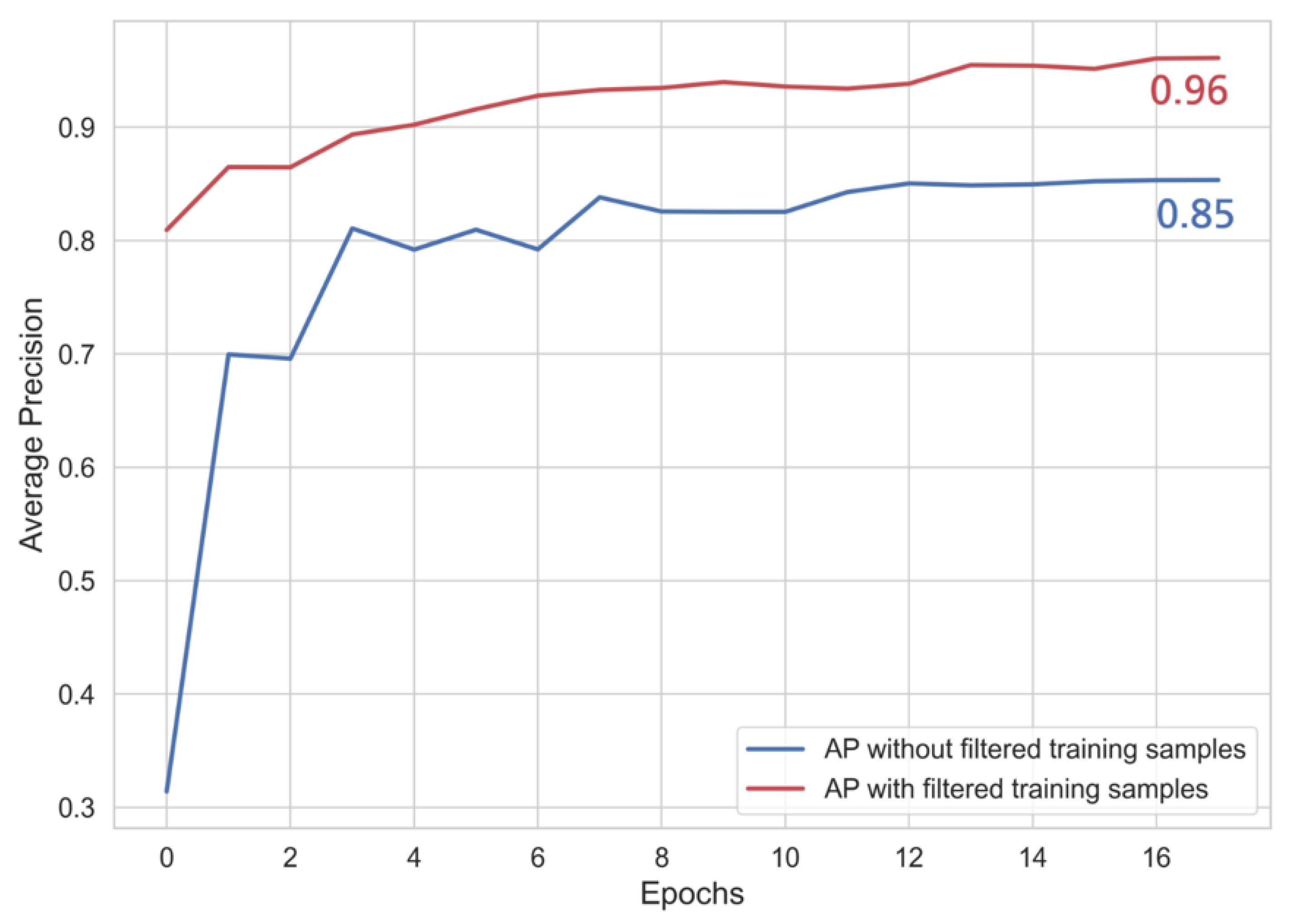
Figure 5.
The figures show the changing losses during training.
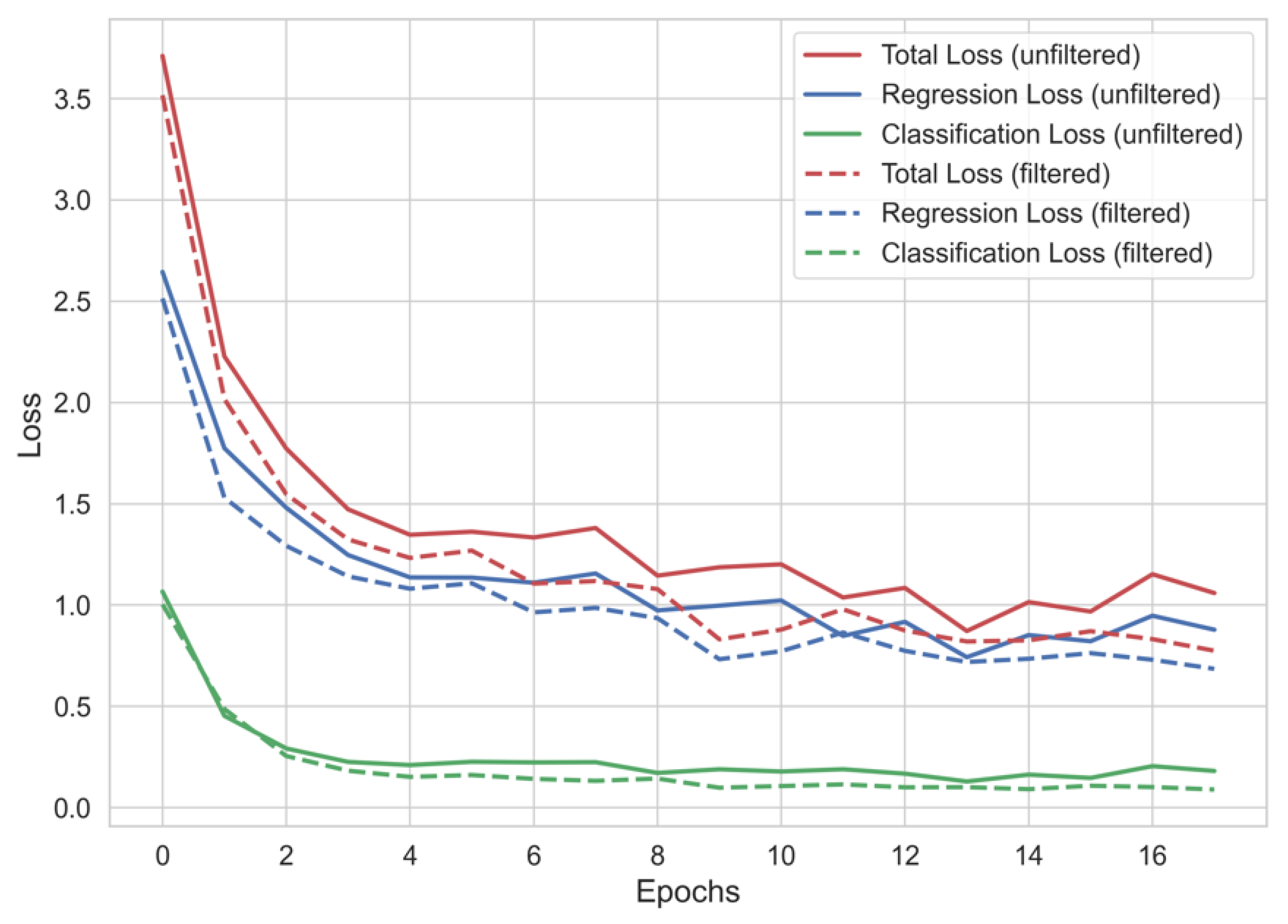
Figure 6.
False positive and false negative examples from the application are summarized in the following. The top row represents incorrectly identified wind turbine, false positives. The bottom row shows turbines that have not been detected.
Figure 6.
False positive and false negative examples from the application are summarized in the following. The top row represents incorrectly identified wind turbine, false positives. The bottom row shows turbines that have not been detected.
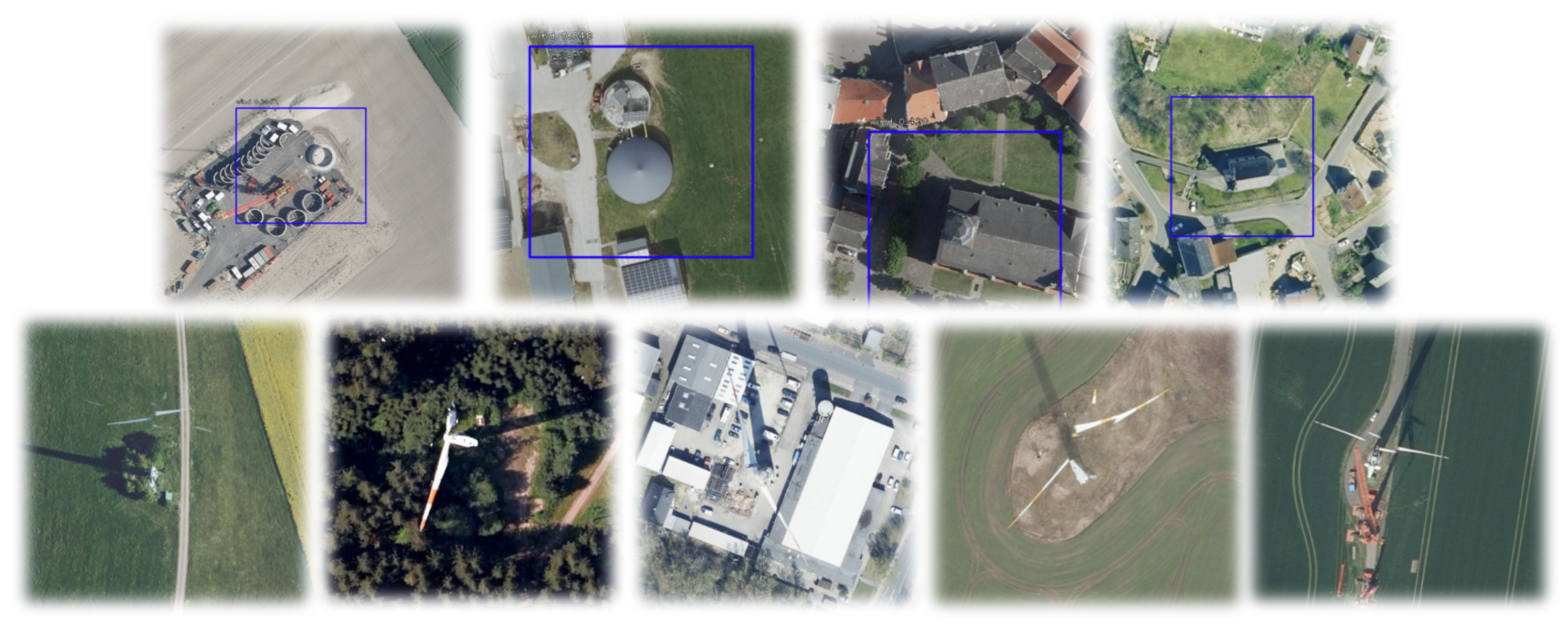
Figure 7.
True positive examples from the application using the DOPs images are presented as follows. The upper row displays instances featuring clearly visible and accurately identified wind turbines, where the centroid of the regression boxes serves as the base of the tower. The bottom row, shows correctly detected wind turbines, with less accurate regressive identification on the images.
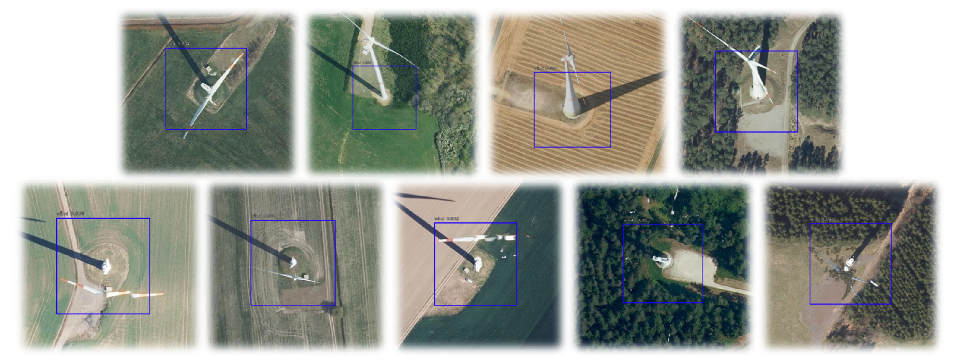
Figure 8.
True positive examples from the application using the Bing images are presented as follows. The upper row displays instances featuring clearly visible and accurately identified wind turbines, where the centroid of the regression boxes serves as the base of the tower. The bottom row, shows correctly identified wind turbines, with less accurate regressive delineation in the images.
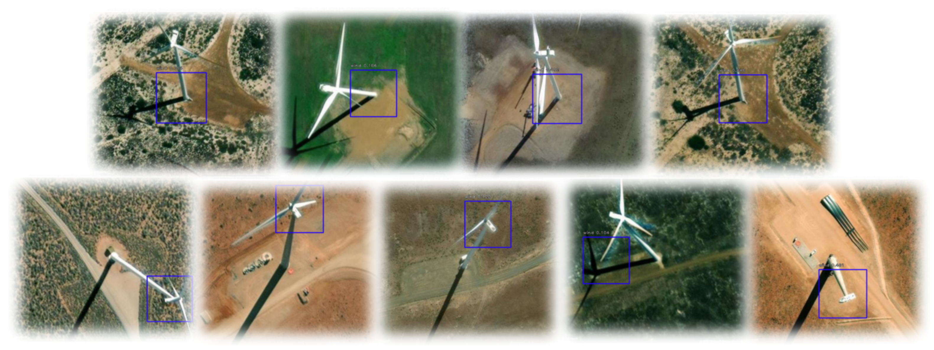
Figure 9.
True positive examples from the application using the Google images are presented as follows. The upper row displays instances featuring clearly visible and accurately identified wind turbines, where the centroid of the regression boxes serves as the base of the tower. The bottom row, shows correctly identified wind turbines, with less accurate regressive delineation in the images.
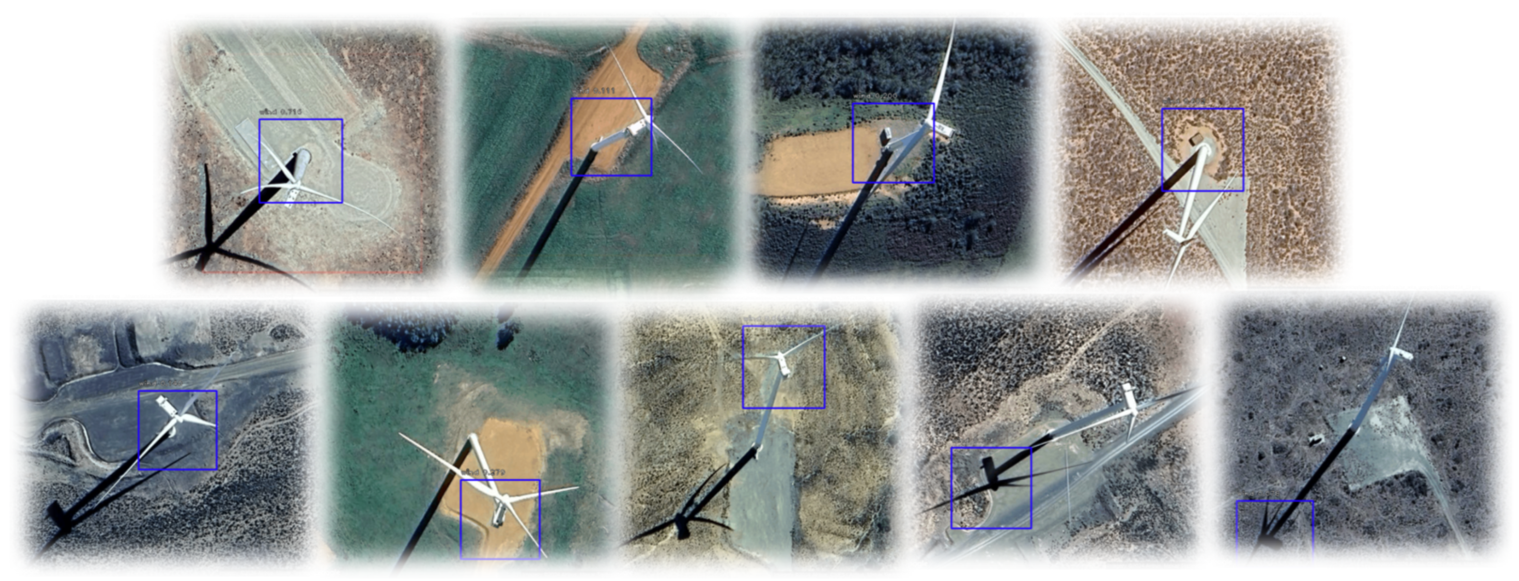
Figure 10.
Histogram of wind turbine location errors based on Bing and Google imagery. It shows the percentage of turbines whose corrected coordinates fall within different distance ranges compared to their original OSM positions.
Figure 10.
Histogram of wind turbine location errors based on Bing and Google imagery. It shows the percentage of turbines whose corrected coordinates fall within different distance ranges compared to their original OSM positions.
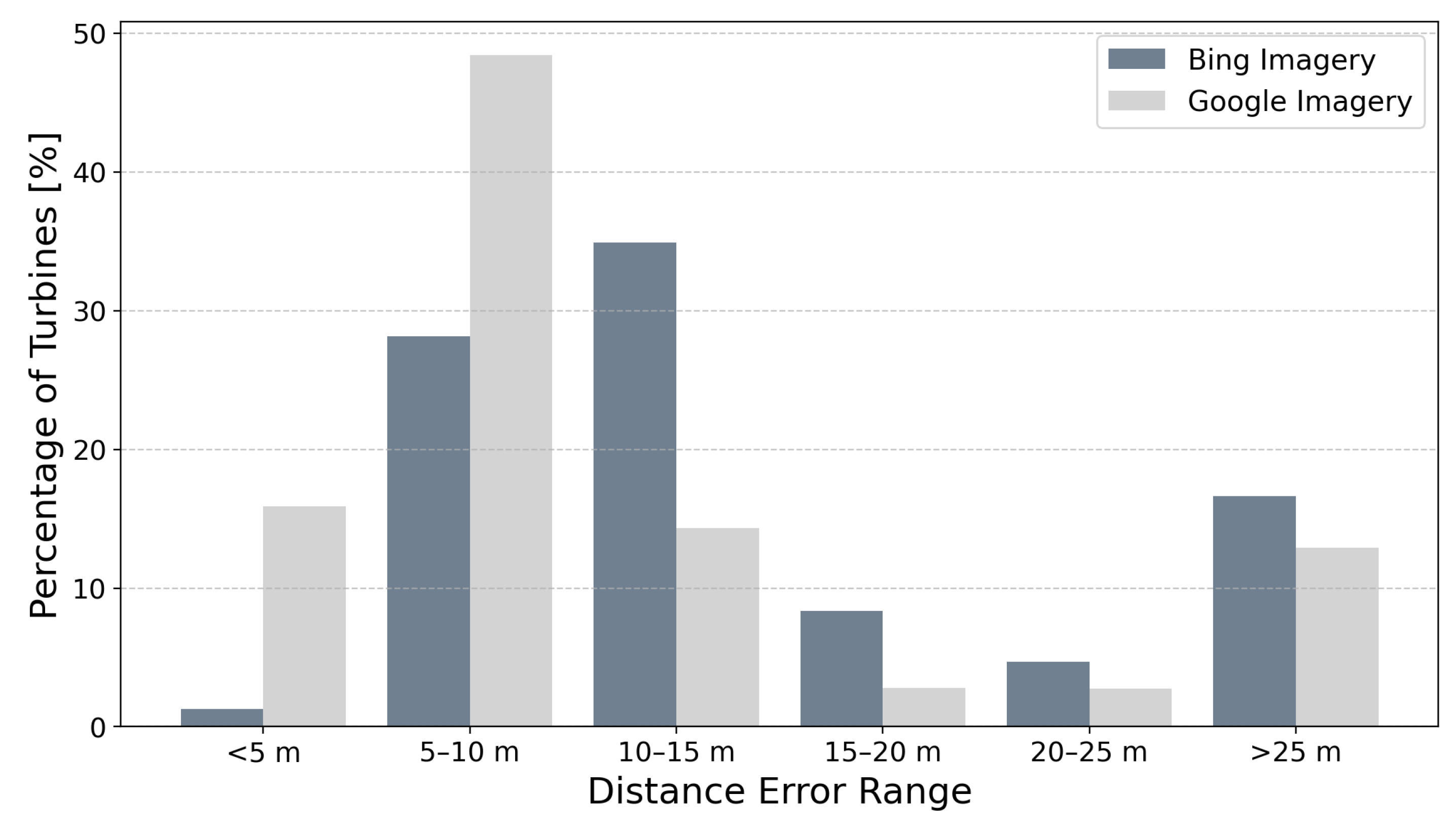
Figure 11.
Summary statistics of key parameters of South African wind farms. Number of turbines per wind farm (left side), total installed capacity (MW) per wind farm (in the middle), and capacity per turbine (MW) (on the left). The boxplots contains the median, interquartile range, and outliers in the dataset
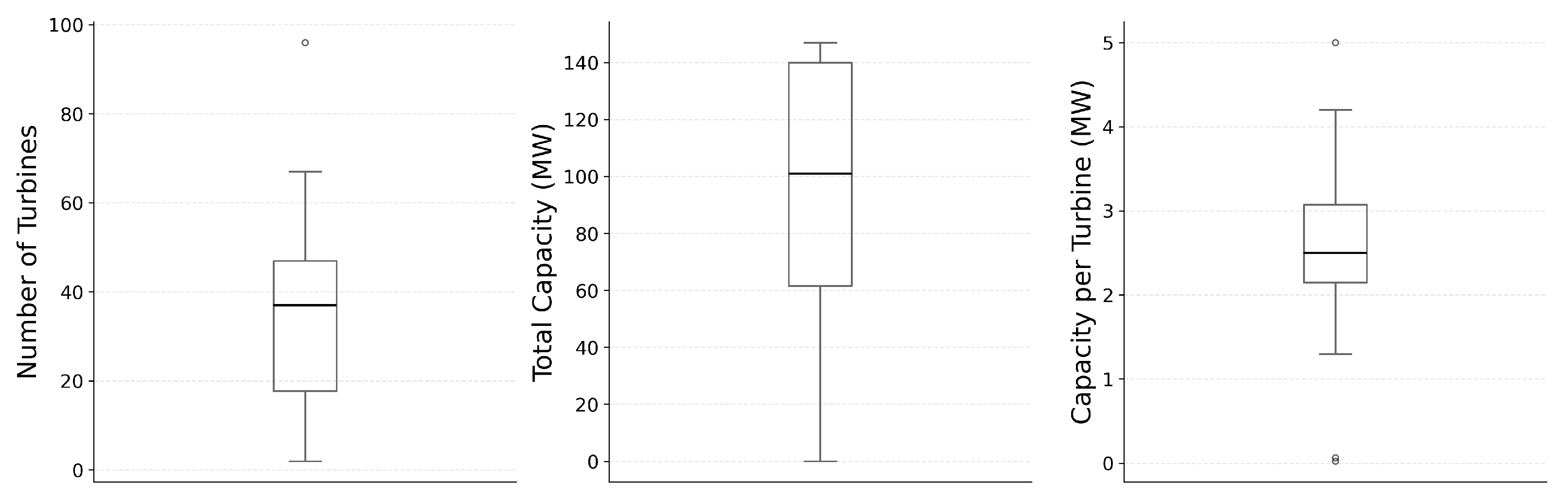
Figure 12.
Development of wind power capacity in South Africa by year. The annual installed wind power capacity from 2008 to 2025 is shown on the left-hand side, and the cumulative installed capacity on the right-hand side.
Figure 12.
Development of wind power capacity in South Africa by year. The annual installed wind power capacity from 2008 to 2025 is shown on the left-hand side, and the cumulative installed capacity on the right-hand side.
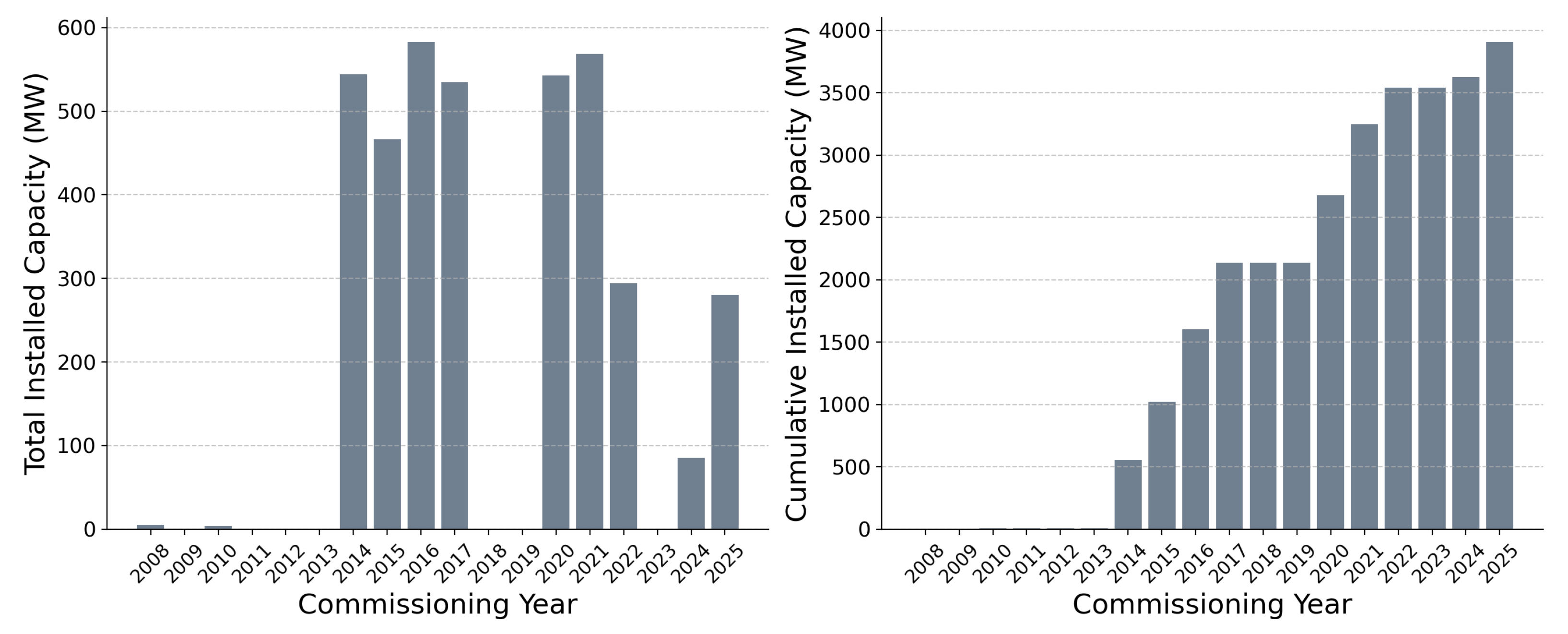
Figure 13.
The total installed capacity (MW) of the individual wind farms is shown. The wind farms are listed by size, starting with the largest.
Figure 13.
The total installed capacity (MW) of the individual wind farms is shown. The wind farms are listed by size, starting with the largest.
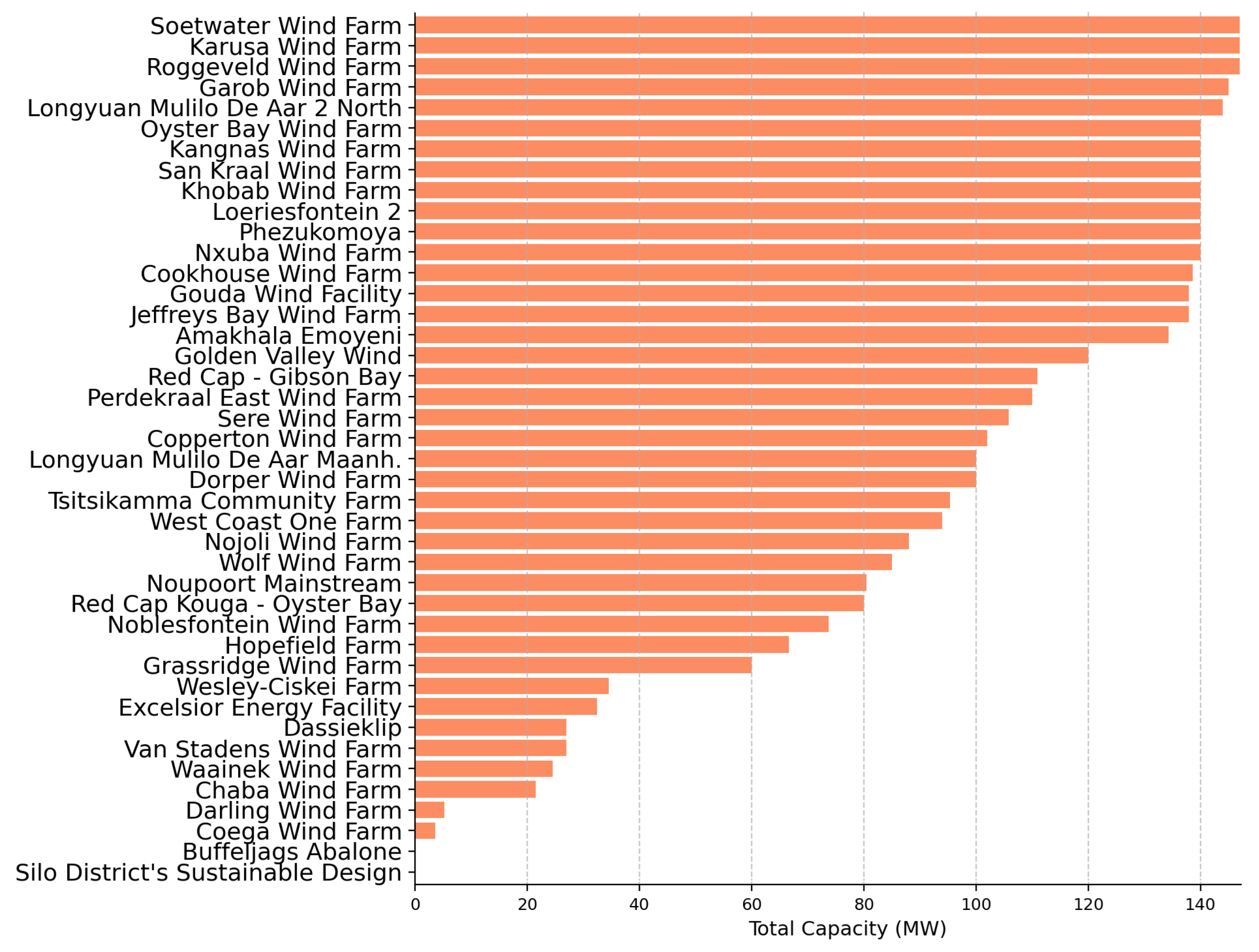
Figure 14.
This figure shows the number of wind turbines per wind farm. Wind farms with more turbines are shown at the top, while smaller farms with fewer turbines are listed further down.
Figure 14.
This figure shows the number of wind turbines per wind farm. Wind farms with more turbines are shown at the top, while smaller farms with fewer turbines are listed further down.
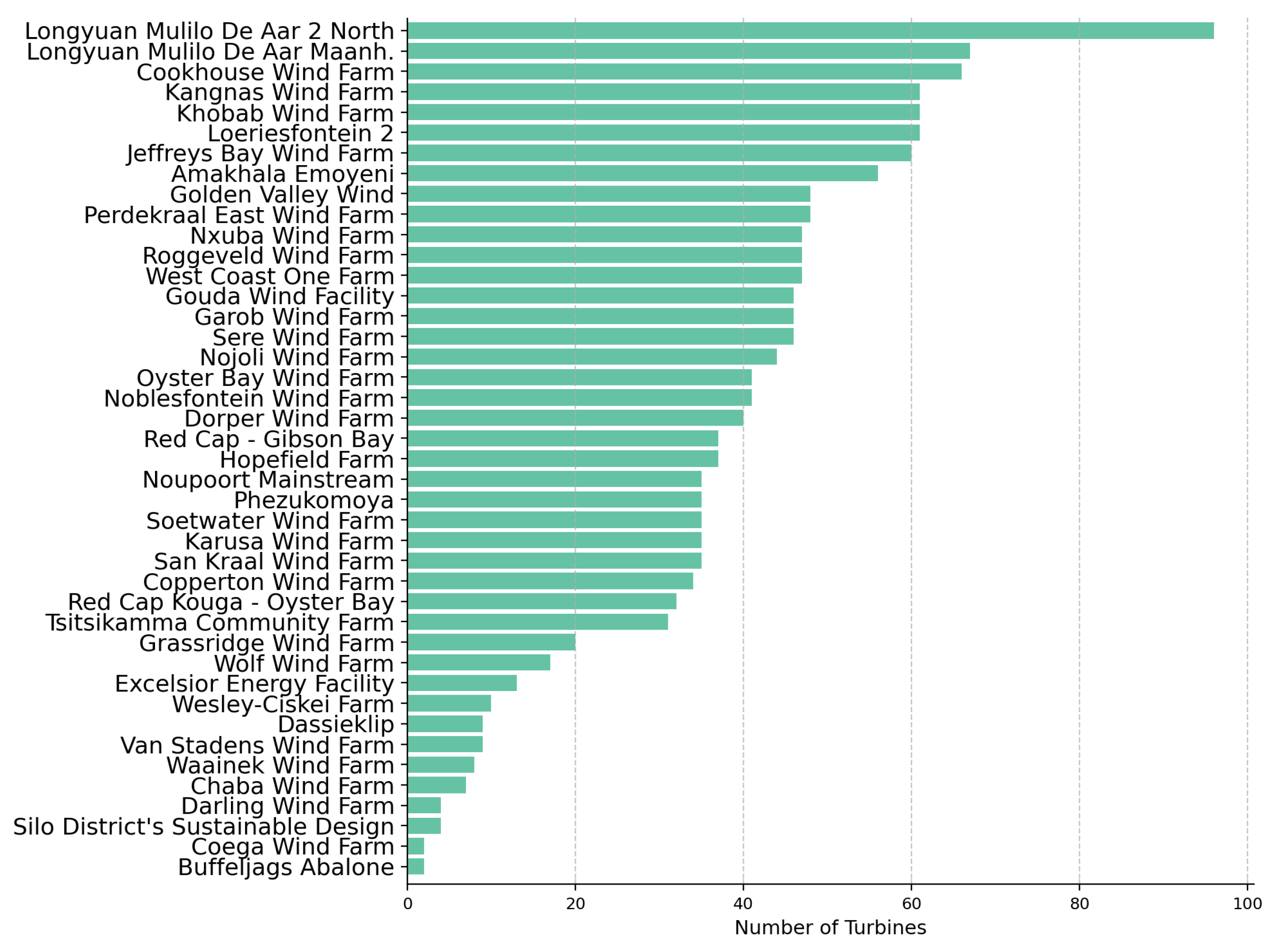
Figure 15.
The capacity per wind turbine in megawatts (MW) for the wind farms in South Africa is shown. The values are sorted in ascending order so that wind farms with a lower capacity per turbine are shown at the bottom and wind farms with a higher capacity at the top.
Figure 15.
The capacity per wind turbine in megawatts (MW) for the wind farms in South Africa is shown. The values are sorted in ascending order so that wind farms with a lower capacity per turbine are shown at the bottom and wind farms with a higher capacity at the top.

Figure 16.
Spatial distribution of all existing wind turbines in South Africa, marked in blue, highlighting their locations across the country.
Figure 16.
Spatial distribution of all existing wind turbines in South Africa, marked in blue, highlighting their locations across the country.

Figure 17.
Spatial distribution of wind energy infrastructure by municipality. Map (on the left side) displays the number of wind turbines, while map (on the right side) shows the total installed wind capacity (MW). The patterns reveal significant regional clustering, with a small number of municipalities concentrating the majority of infrastructure.
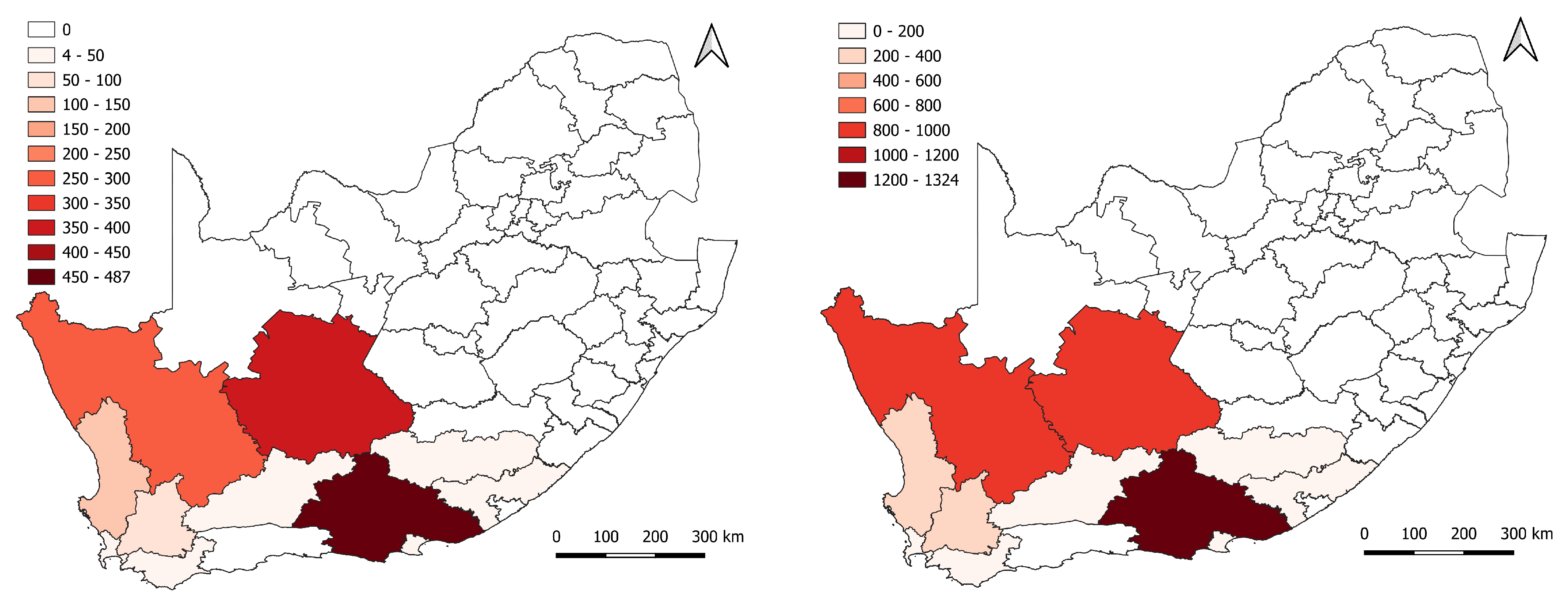

Table 1.
Comparison of onshore wind turbine data distributions across South Africa using Bing images and Google images, including count and percentage of coordinates within different confidence scores.
Table 1.
Comparison of onshore wind turbine data distributions across South Africa using Bing images and Google images, including count and percentage of coordinates within different confidence scores.
| Confidence Score | Bing Count | Bing (%) | Google Count | Google (%) |
|---|---|---|---|---|
| 206 | 13.85 | 116 | 7.80 | |
| 0.1 – 0.2 | 361 | 24.28 | 288 | 19.37 |
| 0.2 – 0.3 | 244 | 16.41 | 223 | 15.00 |
| 0.3 – 0.4 | 182 | 12.24 | 222 | 14.93 |
| 0.4 – 0.5 | 141 | 9.48 | 156 | 10.49 |
| 0.5 – 0.6 | 125 | 8.41 | 144 | 9.68 |
| 0.6 – 0.7 | 85 | 5.72 | 129 | 8.68 |
| 0.7 – 0.8 | 51 | 3.43 | 122 | 8.20 |
| 3 | 0.20 | 45 | 3.03 | |
| NULL | 90 | 6.05 | 43 | 2.89 |
| Total | 1487 | 100.00 | 1487 | 100.00 |
Table 2.
Comparison of wind turbine coordinate deviations in South Africa based on image sources. The percentage of wind turbines that lie within certain distance ranges between the original OSM coordinates and the coordinates corrected using Bing and Google satellite images are shown.
Table 2.
Comparison of wind turbine coordinate deviations in South Africa based on image sources. The percentage of wind turbines that lie within certain distance ranges between the original OSM coordinates and the coordinates corrected using Bing and Google satellite images are shown.
| Distance Range [m] | Bing (%) | Google (%) |
|---|---|---|
| 1.27 | 15.87 | |
| 5–10 | 28.13 | 48.43 |
| 10–15 | 34.90 | 14.33 |
| 15–20 | 8.37 | 2.81 |
| 20–25 | 4.69 | 2.75 |
| >25 | 16.61 | 12.93 |
| Not Detected (NULL) | 6.03 | 2.88 |
Table 3.
Summary of Wind Turbines in South Africa, including the commissioning year, number of turbines, total capacity, capacity per turbine, and turbine type for each wind farm.
Table 3.
Summary of Wind Turbines in South Africa, including the commissioning year, number of turbines, total capacity, capacity per turbine, and turbine type for each wind farm.
| Name of Farm | Comm. Year | Turbines | Tot. Cap. (MW) | Cap./Turbine (MW) | Turbine Type |
|---|---|---|---|---|---|
| Amakhala Emoyeni | 2016 | 56 | 134.4 | 2.4 | Nordex N117/2400 |
| Buffeljags Abalone | 2012 | 2 | 0.13 | 0.065 | Horizontal Axis Turbine |
| Chaba Wind Farm | 2015 | 7 | 21.5 | 3.075 | Vestas V112-3.075 |
| Coega Wind Farm | 2010 | 2 | 3.6 | 1.8 | General Electric GE2.5XL |
| Cookhouse Wind Farm | 2014 | 66 | 138.6 | 2.1 | Suzlon S88/2100 |
| Copperton Wind Farm | 2021 | 34 | 102 | 3.15 | Acciona AW-3150/125 |
| Darling Wind Farm | 2008 | 4 | 5.2 | 1.3 | Fuhrländer FL 1250/62 |
| Dassieklip | 2015 | 9 | 27 | 3 | Sinovel SL 3000/90 |
| Dorper Wind Farm | 2014 | 40 | 100 | 2.5 | Nordex N100/2500 |
| Excelsior Energy Facility | 2020 | 13 | 32.5 | 2.5 | Goldwind GW121/2500 |
| Garob Wind Farm | 2021 | 46 | 145 | 3.15 | Nordex AW125/3150 |
| Golden Valley Wind | 2020 | 48 | 120 | 2.5 | Goldwind GW121/2500 |
| Gouda Wind Facility | 2015 | 46 | 138 | 3 | Acciona AW-3000/100 |
| Grassridge Wind Farm | 2016 | 20 | 60 | 3 | Vestas V112/3000 |
| Hopefield Farm | 2014 | 37 | 66.6 | 1.8 | Vestas V100-1.8 |
| Jeffreys Bay Wind Farm | 2014 | 60 | 138 | 2.3 | Siemens SWT-2.3-101 |
| Kangnas Wind Farm | 2020 | 61 | 140 | 2.3 | Siemens SWT-2.3-108 |
| Karusa Wind Farm | 2021 | 35 | 147 | 4.2 | Vestas V136-4.2 |
| Khobab Wind Farm | 2017 | 61 | 140 | 2.3 | Siemens SWT-2.3-108 |
| Loeriesfontein 2 | 2017 | 61 | 140 | 2.3 | Siemens SWT-2.3-108 |
| Longyuan Mulilo De Aar 2 North | 2017 | 96 | 144 | 1.5 | Guodian UP86/1500 |
| Longyuan Mulilo De Aar Maanh. | 2016 | 67 | 100 | 1.5 | Guodian UP86/1500 |
| Noblesfontein Wind Farm | 2014 | 41 | 73.8 | 1.8 | Vestas V100-1.8 |
| Nojoli Wind Farm | 2016 | 44 | 88 | 2 | Vestas V100-2.0 |
| Noupoort Mainstream | 2016 | 35 | 80.5 | 2.3 | Siemens SWT-2.3-108 |
| Nxuba Wind Farm | 2020 | 47 | 140 | 3 | Nordex AW 125/3150 |
| Oyster Bay Wind Farm | 2021 | 41 | 140 | 3.45 | Vestas V117-3.45 |
| Perdekraal East Wind Farm | 2020 | 48 | 110 | 2.3 | Siemens SWT-2.3-108 |
| Phezukomoya | 2025* | 35** | 140 | 4 | Vestas V136-4.0 |
| Red Cap - Gibson Bay | 2017 | 37 | 111 | 3 | Nordex N117/3000 |
| Red Cap Kouga - Oyster Bay | 2015 | 32 | 80 | 2.5 | Nordex N90/2500 |
| Roggeveld Wind Farm | 2022 | 47 | 147 | 3.15 | Nordex AW125/3150 |
| San Kraal Wind Farm | 2025* | 35** | 140 | 4 | Vestas V136-4.0 |
| Sere Wind Farm | 2015 | 46 | 105.8 | 2.3 | Siemens SWT-2.3-108 |
| Silo District’s Sustainable Design | 2024 | 4 | 0.1 | 0.025 | Vertical Axis Turbine |
| Soetwater Wind Farm | 2022 | 35 | 147 | 4.2 | Vestas V136-4.2 |
| Tsitsikamma Community Farm | 2016 | 31 | 95.325 | 3.075 | Vestas V112-3.0 |
| Van Stadens Wind Farm | 2014 | 9 | 27 | 3 | Sinovel SL 3000/113 |
| Waainek Wind Farm | 2016 | 8 | 24.6 | 3.075 | Vestas V112-3.075 |
| Wesley-Ciskei Farm | 2021 | 10 | 34.5 | 3.45 | Vestas V126-3.45 |
| West Coast One Farm | 2015 | 47 | 94 | 2 | Vestas V90-2.0 |
| Wolf Wind Farm | 2024 | 17 | 85 | 5 | Vestas V162/V163 |
* under construction. ** not all wind turbines have been built yet, thus do not match the detaileddataset.
Table 4.
Overview of wind farms in South Africa by province. The number of different wind farms, the total number of turbines and the aggregated installed capacity are shown.
Table 4.
Overview of wind farms in South Africa by province. The number of different wind farms, the total number of turbines and the aggregated installed capacity are shown.
| Province | Wind Farms | Turbines | Total Capacity (MW) |
|---|---|---|---|
| Eastern Cape | 18 | 575 | 1,571 |
| Northern Cape | 14 | 656 | 1,670 |
| Western Cape | 10 | 256 | 575 |
Disclaimer/Publisher’s Note: The statements, opinions and data contained in all publications are solely those of the individual author(s) and contributor(s) and not of MDPI and/or the editor(s). MDPI and/or the editor(s) disclaim responsibility for any injury to people or property resulting from any ideas, methods, instructions or products referred to in the content. |
© 2025 by the authors. Licensee MDPI, Basel, Switzerland. This article is an open access article distributed under the terms and conditions of the Creative Commons Attribution (CC BY) license (http://creativecommons.org/licenses/by/4.0/).
Copyright: This open access article is published under a Creative Commons CC BY 4.0 license, which permit the free download, distribution, and reuse, provided that the author and preprint are cited in any reuse.


