
Submitted:
07 May 2025
Posted:
07 May 2025
You are already at the latest version
Abstract
Strings are commonly used in engineering structures but are highly susceptible to vibrations due to their low structural stiffness and damping. Suppressing these vibrations poses a significant challenge, as existing tools and technologies are limited. This study investigates the active control of string vibrations through manipulation at one end. To achieve this, a displacement actuator and displacement sensors are considered. Based on the characteristics of actuator and sensor, a multi-modal position-input position-output control algorithm is proposed. Both theoretical analysis and experimental results demonstrate that the proposed control method effectively suppresses multi-mode string vibrations.
Keywords:
active vibration control of string
; position–input position–output control
; modal space control
; verification by experiments
1. Introduction
Passive-type dampers are the simplest means of controlling string vibration [1]. Semi-active vibration control has also been proposed for more flexible control. This approach adjusts damping in real-time based on feedback signals, offering advantages like adaptability to changing conditions, and reduced power consumption compared to active control systems. Numerous studies have explored semi-active control techniques for string vibration, aiming to optimize performance, while minimizing energy consumption and system complexity [2,3].
Active vibration control is essential to achieve superior performance in controlling string vibrations. However, string structures are often installed at elevated positions, which makes it difficult to apply control forces to the middle part of the string. Therefore, it is ideal to make one end of the string movable so that force can be applied. The control method born from this motivation is boundary control. The boundary control, which involves applying control inputs near the boundaries of the system to control vibrations, has been widely studied. Baicu et al. [4] used a modified Lyapunov method for the vibration control of cables, demonstrating control performance through simulations and experiments. He et al. [5] investigated adaptive boundary control for a flexible string system considering parameter uncertainties, while He and Ge [6] explored model-based and adaptive boundary feedback control. Most boundary control methods are based on Lyapunov’s method, which requires measurements of displacement and velocity at the boundary. The velocity information can be derived mathematically by taking the derivative of displacement. But in practice, the noise involved in the displacement signal may cause problems in the differentiation process.
Different control algorithms have been applied to boundary control. Zhao et al. [7] proposed adaptive neural-network-based fault-tolerant control, Fujino et al. [8] implemented active stiffness control using piezoelectric actuators, while Alsahlani and Mukherjee [9] utilized a scabbard-like actuator for control. Li et al. [10] demonstrated controllers using energy harvesting-based self-powered active control, and a Linear Quadratic Gaussian (LQG) controller.
Unlike other structures, strings exhibit significant resonance across both low-order and higher-order modes, due to their very low damping. Most studies on the active vibration control of strings have focused on single-input single-output control, but controllers capable of suppressing multiple natural modes are needed. Additionally, most of the studies mentioned above are numerical analyses, and there are very few studies that prove the validity of proposed control algorithms through experiments.
This study assumed that one end of the string is fixed and the other end is movable. And it assumed that the displacement of the other end is controlled by internal feedback control. In other words, it is assumed that we can accurately follow the desired displacement using a servo motor. Since the actual control of the servo motor is driven in this way, it is more reasonable than applying force.
This study proposes an extended Position–input Position–output (PIPO) controller as the active vibration controller. The effectiveness of the proposed controller is validated through both numerical analysis and experiments, aiming to bridge the gap between theoretical studies and practical applications in string vibration control.
2. Equations of Motion for String with End-Displacement Actuation
Consider a uniform string of length , as shown in Figure 1. Assume that the point where undergoes rectilinear motion, , along the –axis and the other end at is fixed. represents the relative displacement of the string with respect to . We aim to control the vibration of the string by using and the proposed control algorithm.
The kinetic energy and elastic energy, and virtual work of the string shown in Figure 1 can be written as follow:
where , represents the mass per unit length of the string, denotes tension, and is the distributed external force acting along , while and denote the virtual work and virtual displacement, respectively.
The assumed mode method is used as a numerical analysis technique. By discretizing the string displacement into a discrete system of multiple degrees of freedom using a non-dimensionless variable in the length direction, the string displacement can be expressed as follows:
where, is a matrix composed of admissible functions for string displacement, and is a generalized displacement vector of size , where denotes the number of admissible functions. Assuming that the string is uniform, and using Equations (1) and (5), Equations (2-4) can be expressed as follow:
where , and
To derive the equations of motion, the following Lagrange equation is used:
where . By inserting Equations (6-8) into Equation (10), the following equations of motion can be derived:
The admissible functions of the assumed mode method utilize the eigenfunctions of a string with both ends fixed, and are as follow:
In fact, these functions are the eigenfunctions of a uniform string. Inserting Equation (12) into (9), we can obtain.
where is an identity matrix and is an zero matrix. Dividing Equation (11) by and using Equation (13), we can rewrite Equation (11) as follows:
where the modal damping matrix is added, is an matrix composed of damping ratios, and
Looking at Equation (14), we can see that since we consider a uniform string, we obtain a decoupled modal equation of motion. However, the only controller we can use is a displacement controller attached to the end. In this case, the control algorithm becomes a Multiple-Input Single-Output (MISO) system. However, since it is not easy to develop a control algorithm in the form of MISO, it is desirable to develop a control algorithm that can tackle each modal coordinate independently.
First, let's assume that we have modal control forces and that we use these control forces to control modal coordinates. Of course, . Since the sum of the outputs of each controller corresponds to the actual displacement of the moving end, we can express the final end-displacement as follows:
where is an matrix consisting of ones, is an vector consisting of the outputs of each controller. Then, the equations of motion, Equation (14) can be rewritten as follows:
When using Equation (17), since is a vector and is a vector, the number of controllers is insufficient. Therefore, when performing control, a control spillover problem to a high-order mode occurs. However, this problem is not limited to the vibration control problem of the string dealt with in this study, but is a problem that always appears in the vibration control of a flexible structure with infinite degrees of freedom. Fortunately, since the damping for the high-order modes is large, solving the low-order vibration problem becomes a major task.
3. The Position–Input Position–Output Control Algorithm
Equation (17) represents the equation of motion when modal coordinates are controlled by actuators. Looking at the equation of motion given by Equation (17), we can see that the base displacement as an actuating force vector, and the modal displacement is generated by this force and an external disturbance force . Our task is to design a control algorithm that can generate an appropriate control displacement using the sensor value of . Therefore, the control algorithm naturally results in the Position-Input Position-Output (PIPO) control algorithm.
There are not many PIPO control algorithms for vibration control. The only notable research on this topic is the PIPO control algorithm proposed by Kim et al. [11]. The vibration system dealt with in [11] is a system in which an actuator and a spring-damper are connected in series, but has different equations of motion compared to the system considered in this study.
Before solving the vibration control problem of a multi-degree-of-freedom system, let us first consider the problem of a single-degree-of-freedom vibrating system. Based on Equation (17), the equation of motion of a single-degree-of-freedom vibrating system can written as follows.
where , is generalized coordinate, is damping ratio, is gain, can be regarded as control displacement, is external disturbance, respectively. Unlike Equation (17), the time variable was non-dimensionalized using to eliminate frequency dependency.
In this study, we propose the use of the following compensator equation to control the equation of motion given by Equation (18).
where is the damping factor of the compensator. A controller of the form of equation (19) has already been used in reference [11]. However, the equation of motion of the system treated in reference [11] is different from Equation (18). However, as suggested in reference [11], we may expect that a control equation of the form of Equation (19) can be useful, and let us analyze what happens when this control algorithm is applied. The equation for the closed-loop control system given by Equations (18) and (19) can be combined and expressed as the following matrix ordinary differential equation.
Using the Laplace transform, Equation (20) is derived as follows.
where , , . The characteristic equation of Equation (21) can be derived as:
Applying the Routh-Hurwitz stability criterion to Equation (22), we can see that it is unconditionally stable if . This result is a bit different from the result in reference [11] that states that a given system is stable only if , because the equation of motion given by Equation (18) is different from the equation of motion dealt in reference [11]. The stability condition such as is a condition that is advantageous to the user when designing a controller. However, the question remains as to which gain value should be used. To this end, we calculated the root-locus by setting , and changing the gain from 0 to 1, and the result is as shown in Figure 2. Looking at Figure 2, we can see that as the gain increases, the two roots become negative and move away from the imaginary axis, and then approach the imaginary axis again. Therefore, we can see that it is not desirable to unconditionally increase the gain. Then, the question remains as to how much gain should be used. Figure 3 shows the maximum real part of the system poles as a function of gain. From Figure 3, we can see that the gain reaches its minimum value at around 0.3.
Now let us return to the equation of motion of the multi-DOF system, Equation (17). To control modal displacements, at least displacement sensor values are required. And we will assume sensors are available. This implies that we consider the same number of equations of motion to be controlled as the number of sensors. In practice, it is not possible to use a large number of sensors to measure all modal displacements, so it should be kept in mind that a limited number of sensors are used. If we assume that m modal displacements can be measured and estimated by displacement sensors, we can propose a compensator equation for Equation (17) based on Equation (19) as follows:
where is a matrix composed of gains, is a matrix composed of damping ratios of the controllers and is a sub-vector extracted from the original vector, containing components. Hence, we may write:
where
Using Equations (17), (23), and (24), the matrix equation for the following closed-loop system can be obtained:
4. Sensor Measurement
To compute using the compensator equation, Equation (23), is needed. However, it is impossible to measure directly. In reality, we can measure only the absolute displacement of the string at the sensor points because the laser displacement sensors are mounted on the ground. Let be the vector composed of absolute displacements measured by the sensors. Then, the relationship between and can be expressed as follows, using Equations (1) and (5):
where
Note that the modal displacement is truncated in Equation (24). In this case, an observer spillover problem occurs. Like the control spillover problem, this problem is inevitable, as it is impossible to measure all modal displacements for vibration control of a flexible structure with infinite degrees of freedom.
In practical controller implementation, a process is required to convert to using Equation (27) so that the following equation can be used to estimate the elastic displacements.
5. Numerical Analysis
Table 1 presents the properties of the string obtained from the string used in experiments. The natural frequencies of the string up to the third mode calculated by using the data of Table 1 are 2.95, 5.91, and 8.86 Hz.
To evaluate the control performance of the proposed MIMO PIPO control algorithm given by Equation (23), the frequency response functions of the uncontrolled and controlled systems were computed. In the numerical analysis, it is assumed that the point of applied disturbance is the same as the point of measurement.
The closed-loop block diagram for the addressed problem can be constructed as shown in Figure 4. This block diagram is also used for the construction of the controller in the experiment.
Figure 5 shows the frequency response functions of the uncontrolled and controlled systems. As shown in Figure 5, the first, second, and third natural modes are suppressed as designed. And it can be seen that the other higher modes are not affected by the control of the lower modes. That is, the control spillover problem does not occur. Therefore, it was confirmed that the control methodology developed in this study can be effectively used for the vibration suppression of the string. Figure 6 shows the impulse response, which shows that the vibration is suppressed even though all modes are excited.
6. Experiments
Even if the validity of the control algorithm is proven through theory and numerical calculations, it is necessary to prove that control is possible using an actual string. An experimental device such as Figure 7 was constructed to control the vibration of the string.
The top of the string was fixed to the ceiling, while the bottom was secured to a linear motor. The displacement of the string was measured using a laser displacement sensor (FUWEI Model FSD22-100P), while the base was moved using a linear servo motor (Mitsubishi Electric Model LM-H3P2A-07P-BSS0). Displacement measurements were taken at , considering these as the points where the displacement amplitudes for the first, second, and third modes, respectively. The control algorithm proposed in this study was downloaded to MicroLabBox of dSpace Inc. The output of the control algorithm given by Equation (23) is the position of the end. Therefore, in order to make the position of the linear servo motor be at the calculated position in real time, the servo motor driver is set to the speed mode, and the position of the servo motor measured by the encoder is compared with the desired position, and the error obtained is provided to the PID control algorithm, which calculates an appropriate speed change and provides it to the motor driver. For a control method that can accurately track the position in real time using a linear servo motor, refer to reference [12].
In the experiment, since the absolute displacement is measured, it is necessary to transform it into using Equation (29). Figure 8 shows the Simulink block diagram of the controller for the experiment. Through free vibration experiments, the natural frequencies of the string were confirmed to be (2.95, 5.9, and 8.9) Hz and each PIPO controllers were tuned to each natural frequency. The gains of the controller were all set to 0.15, which were determined through trial and error during the experiment.
To compare the control performance when multiple modes are simultaneously excited, we conducted experiments by applying an impact at the point. Figure 9 shows the uncontrolled and controlled vibration response when an impact is applied. From Figure 9, it can be seen that when the control algorithm proposed in this study is operated, the vibration caused by the initial impact is quickly suppressed. This experimental result is very similar to the numerical calculation result shown in Figure 6.
Figure 10 shows that the vibration due to impact can be quickly suppressed when the control algorithm proposed in this study is used, but the control performance for each natural mode needs to be confirmed again. Therefore, experiments were conducted to see whether the control performance shown in Figure 7 is the same in the experiment when each natural mode is excited and the controller is driven. To this end, an experiment was designed to initially excite harmonically at the target natural frequency and then change the mode to the vibration control mode, and the response was measured.
Figure 10 shows the vibration response measured by the first laser sensor installed at position when excited at the first natural frequency mode. Figure 11 shows the vibration response measured by the second laser sensor installed at position when excited at the second natural frequency mode. Figure 12 shows the vibration response measured by the third laser sensor installed at position when excited at the third natural frequency mode. To prevent shocks to the motor and ensure system stability, the controller signal, when activated, gradually increases over a 2 second period. The experimental results confirm that the MIMO PIPO controller proposed in this study effectively controls up to the third natural mode, as in the case of numerical simulations. The presence of very small residual vibrations in the controlled state is due to the input voltage being lower than the servo motor’s minimum input voltage, resulting in a dead band in the servo motor, which implies that it is not easy to control low-amplitude higher natural modes.
7. Conclusions
In this study, we investigated the active vibration control of a string with one end fixed, and a displacement-type actuator attached to the opposite end. Based on the derived equations of motion, the PIPO control algorithm is proposed in this study for the vibration suppression of string.
Before presenting the MIMO PIPO control algorithm, we tested the SISO PIPO control algorithm by considering a simple 1-DOF vibration system. Using this simple system and controller, we analyzed the stability of the closed-loop system and obtained the result that the closed-loop control system is unconditionally stable if the gain is a positive number greater than 0. Therefore, we can say that users can use this controller with confidence, and further investigation shows that there is an optimal gain.
Based on the theoretical research results for the SISO system, a MIMO PIPO control system was developed. The MIMO PIPO control algorithm is capable of suppressing the vibration of the string by sensing the string’s displacements, and controlling the displacement of a displacement-type actuator. The MIMO PIPO algorithm consists of a sum of controllers designed in modal coordinates. To validate the performance of the controller, numerical analysis and experiments were conducted on a flexible string with one end connected to an actuator. Using three displacement sensors, we aimed to control the displacement up to the third natural mode. Both numerical and experimental results demonstrate that the proposed MIMO PIPO controller can effectively suppress the multi natural modes of the string.
Author Contributions
Conceptualization, M.K.K. and S.-M.K.; methodology, S.-M.K.; software, S.-M.K.; validation, S.-M.K. and M.K.K.; formal analysis, S.-M.K.; investigation, S.-M.K.; resources, M.K.K.; data curation, S.-M.K.; writing—original draft preparation, S.-M.K.; writing—review and editing, S.-M.K. and M.K.K.; visualization, S.-M.K.; supervision, M.K.K.; project administration, M.K.K. All authors have read and agreed to the published version of the manuscript.
Funding
This research received no external funding.
Conflicts of Interest
The authors declare no conflicts of interest.
References
- Lu, L.; Duan, Y.-F.; Spencer, B.F., Jr; Lu, X.; Zhou, Y. Inertial mass damper for mitigating cable vibration. Struct. Control Health Monit. 2017, 24, e1986. [Google Scholar] [CrossRef]
- Johnson, E.A.; Christenson, R.E.; Spencer, B.F. Jr. Semiactive damping of cables with sag. Comput.-Aided Civ. Infrastruct. Eng. 2003, 18, 132–146. [Google Scholar] [CrossRef]
- Ni, Y.Q.; Chen, Y.; Ko, J.M.; Cao, D.Q. Neuro-control of cable vibration using semi-active magneto-rheological dampers. Eng. Struct. 2002, 24, 295–307. [Google Scholar] [CrossRef]
- Baicu, C.F.; Rahn, C.D.; Nibali, B.D. Active boundary control of elastic cables: Theory and experiment. J. Sound Vib. 1996, 198, 17–26. [Google Scholar] [CrossRef]
- He, W.; Zhang, S.; Ge, S.S. Adaptive boundary control of a nonlinear flexible string system. IEEE Trans. Control Syst. Technol. 2014, 22, 1088–1093. [Google Scholar] [CrossRef]
- He, W.; Ge, S.S. Vibration control of a flexible string with both boundary input and output constraints. IEEE Trans. Control Syst. Technol. 2015, 23, 1245–1254. [Google Scholar] [CrossRef]
- Zhao, Z.; Ren, Y.; Mu, C.; Zou, T.; Hong, K.S. Adaptive neural-network-based fault-tolerant control for a flexible string with composite disturbance observer and input constraints. IEEE Trans. Cybern. 2022, 52, 12843–12853. [Google Scholar] [CrossRef] [PubMed]
- Fujino, Y.; Warnitchai, P.; Pacheco, B.M. Active stiffness control of cable vibration. J. Appl. Mech. 1993, 60, 948–953. [Google Scholar] [CrossRef]
- Alsahlani, A.; Mukherjee, R. Vibration control of a string using a scabbard-like actuator. J. Sound Vib. 2011, 330, 2721–2732. [Google Scholar] [CrossRef]
- Li, J.-Y.; Shen, J.; Zhu, S. Adaptive self-powered active vibration control to cable structures. Mech. Syst. Signal Process. 2023, 188, 110050. [Google Scholar] [CrossRef]
- Kim, S.-M.; Kim, D.W.; Kwak, M.K. Design and implementation of an active vibration control algorithm using servo actuator control installed in series with a spring-damper. Appl. Sci. 2023, 13, 3349. [Google Scholar] [CrossRef]
- Talib, E.; Shin, J.-H.; Kwak, M.K. Designing multi-input multi-output modal-space negative acceleration feedback control for vibration suppression of structures using active mass dampers. J. Sound Vib. 2019, 439, 77–98. [Google Scholar] [CrossRef]
Figure 1.
String model of one end undergoing linear motion.
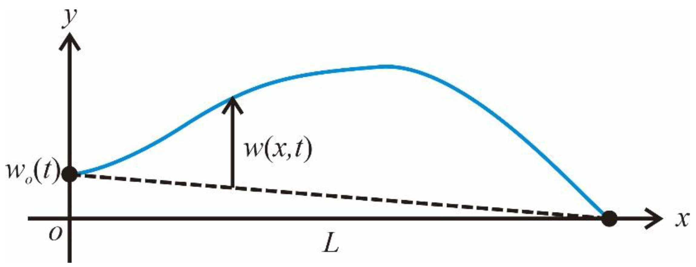
Figure 2.
Root-locus of closed-loop system.
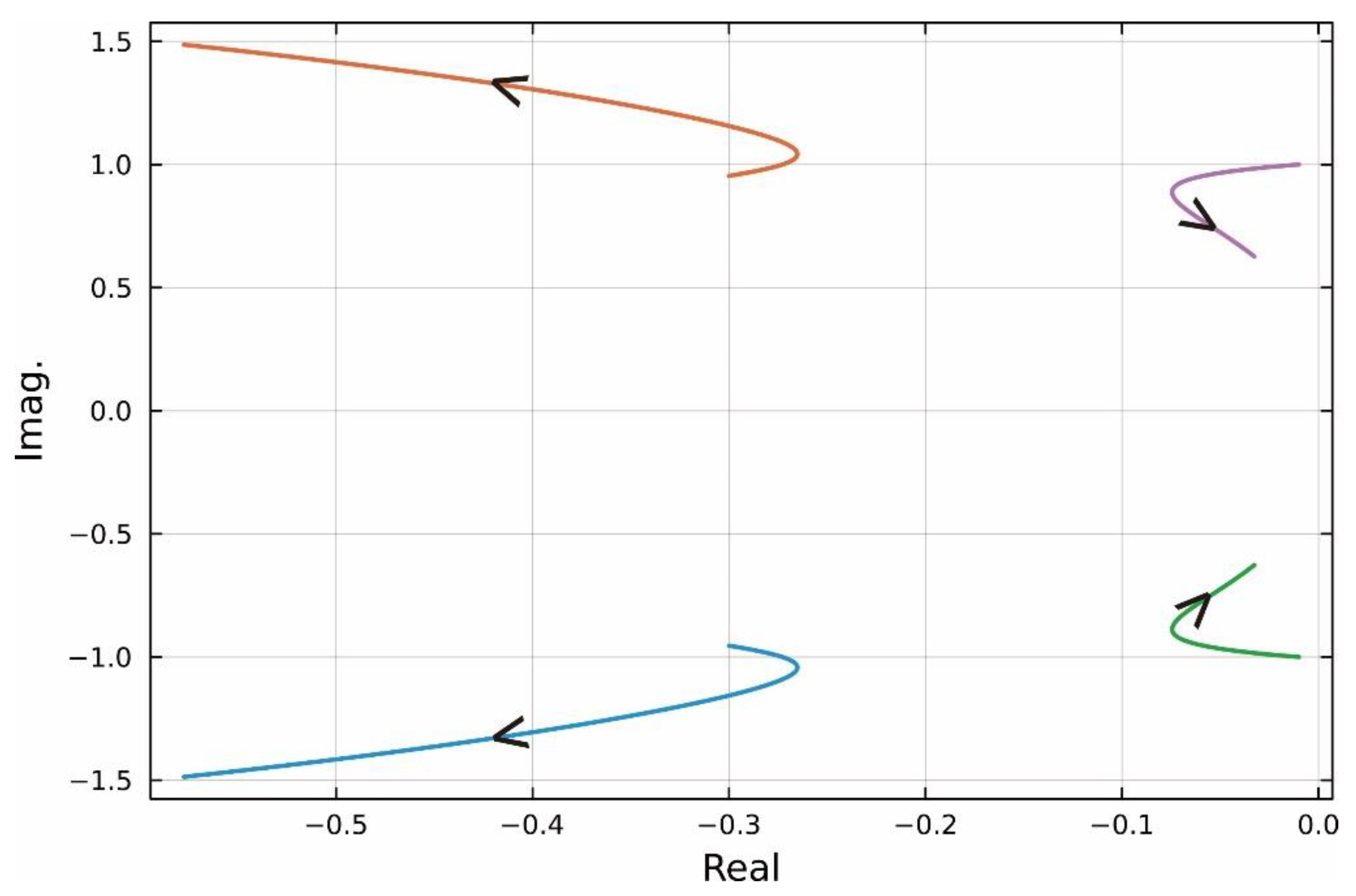
Figure 3.
Maximum of real parts of roots.
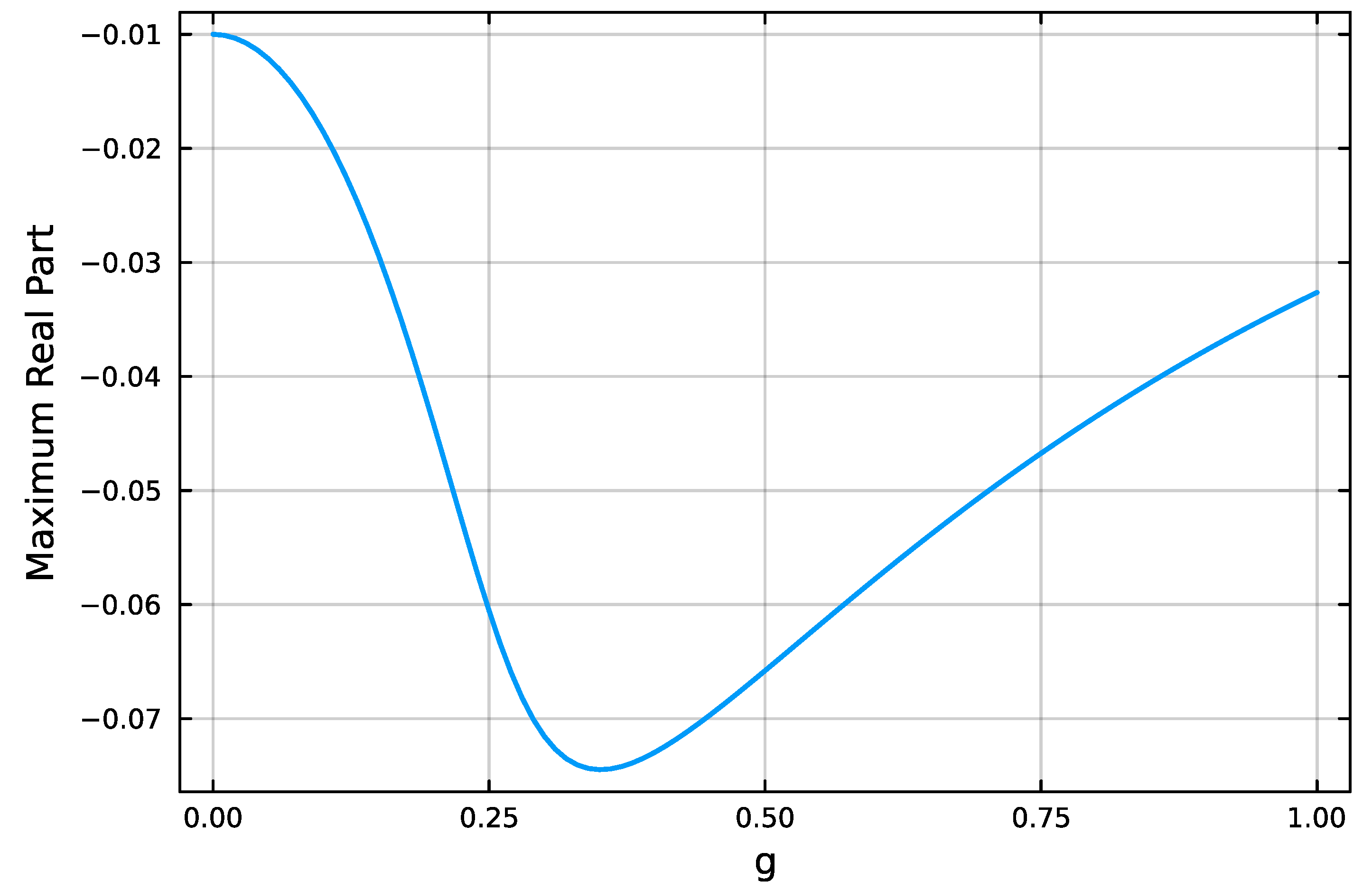
Figure 4.
Block diagram of the closed-loop system.
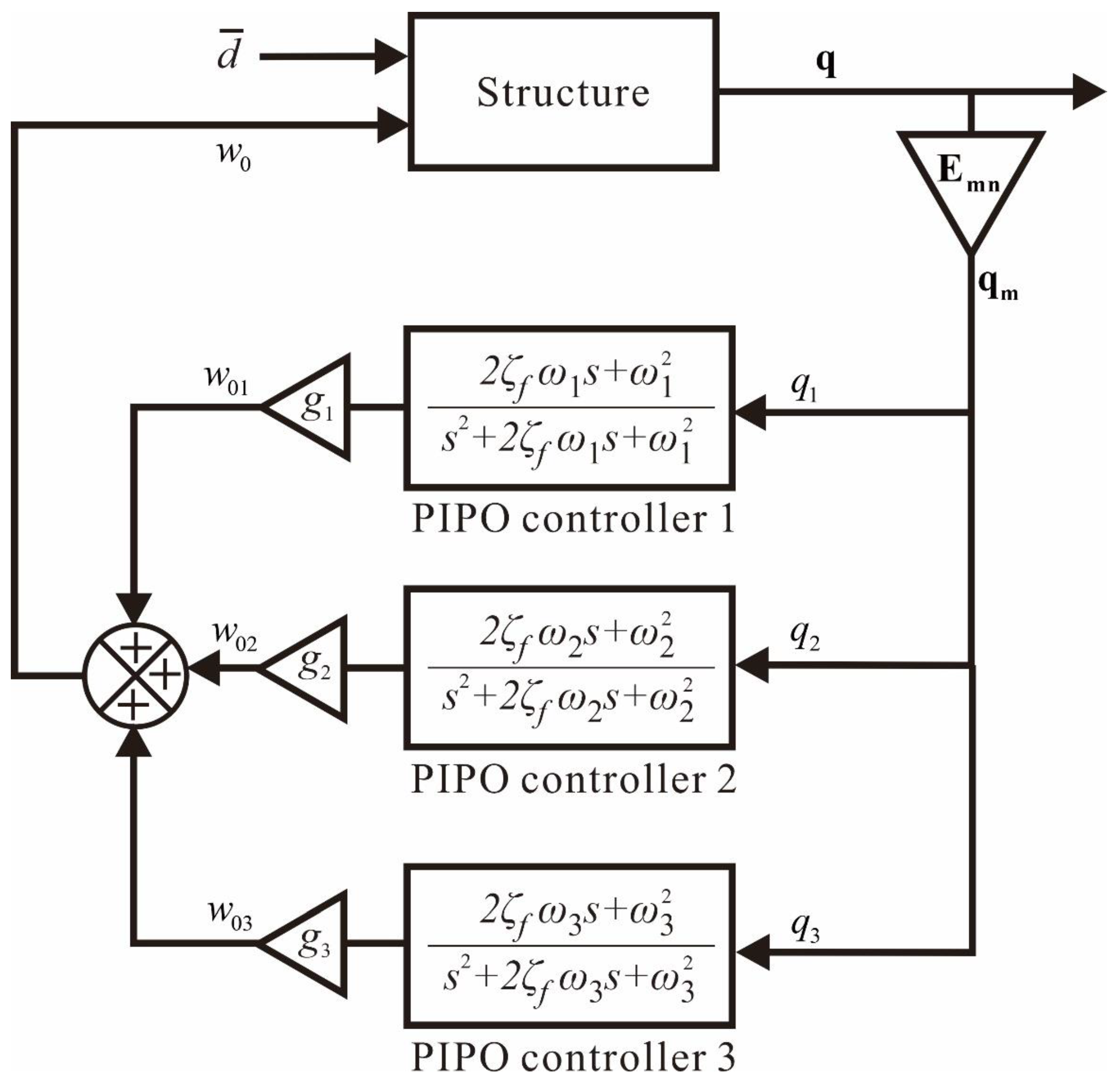
Figure 5.
Uncontrolled and controlled frequency response functions.
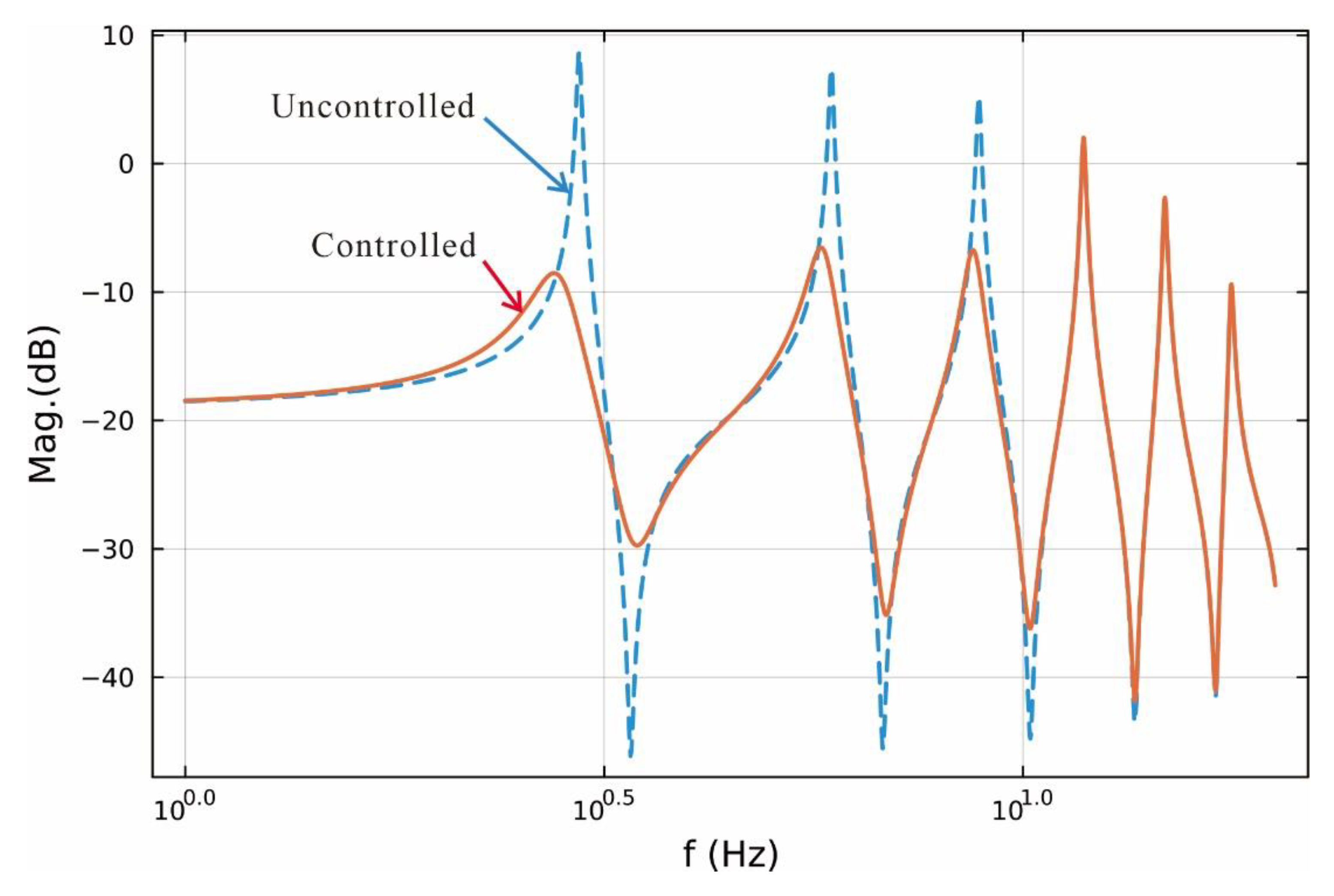
Figure 6.
Uncontrolled and controlled frequency response functions.
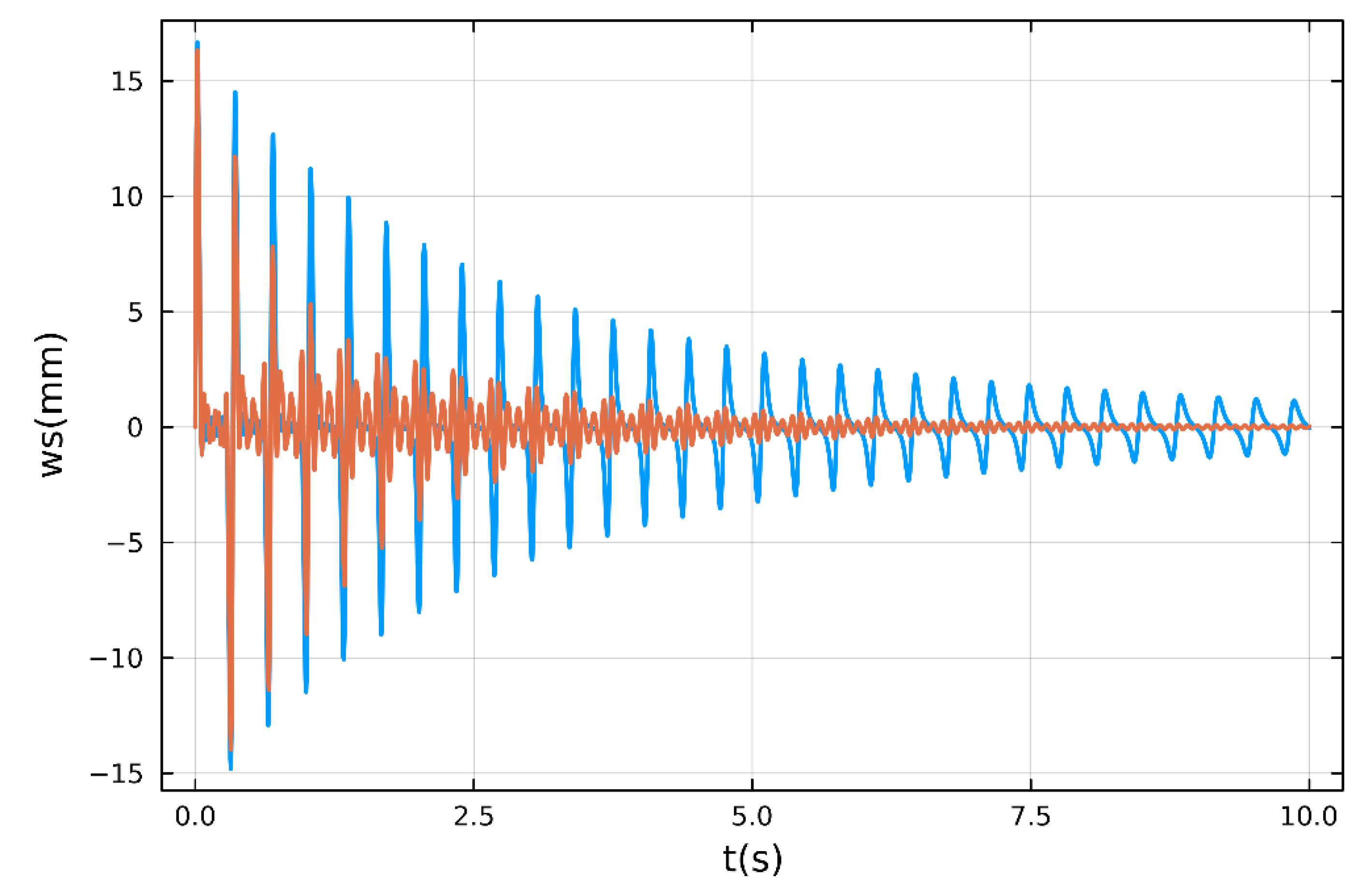
Figure 7.
Experimental testbed and wiring diagram.
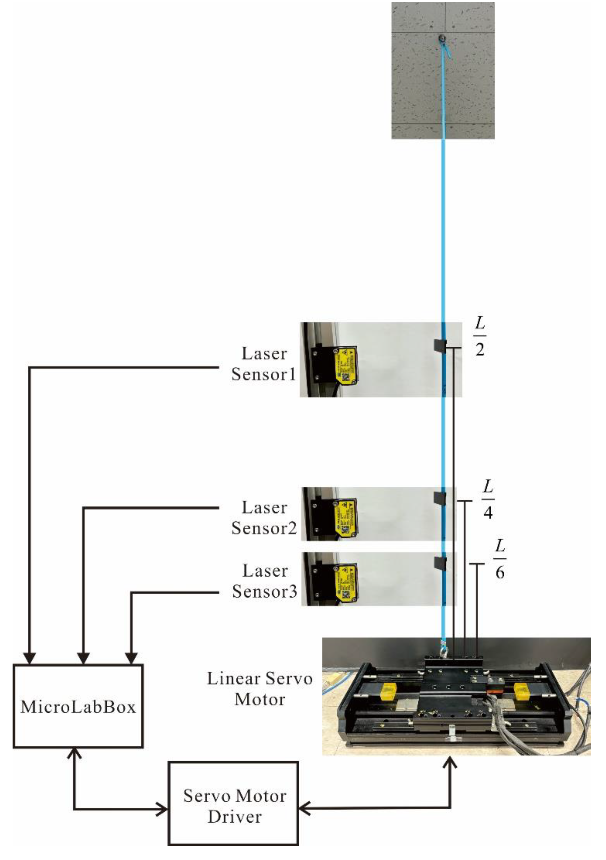
Figure 8.
Simulink block diagram for MIMO PIPO control.
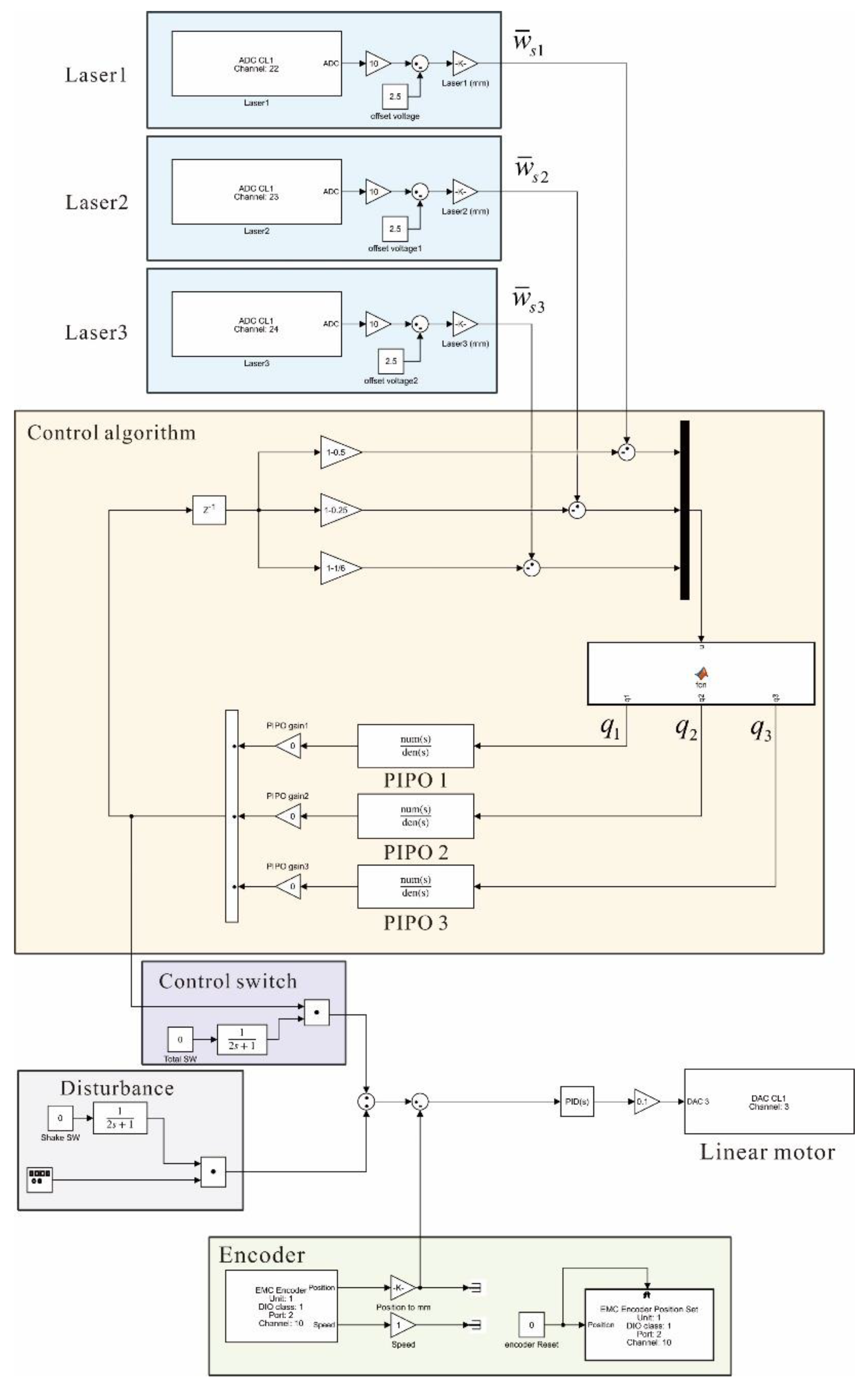
Figure 9.
Experimental impulse response.
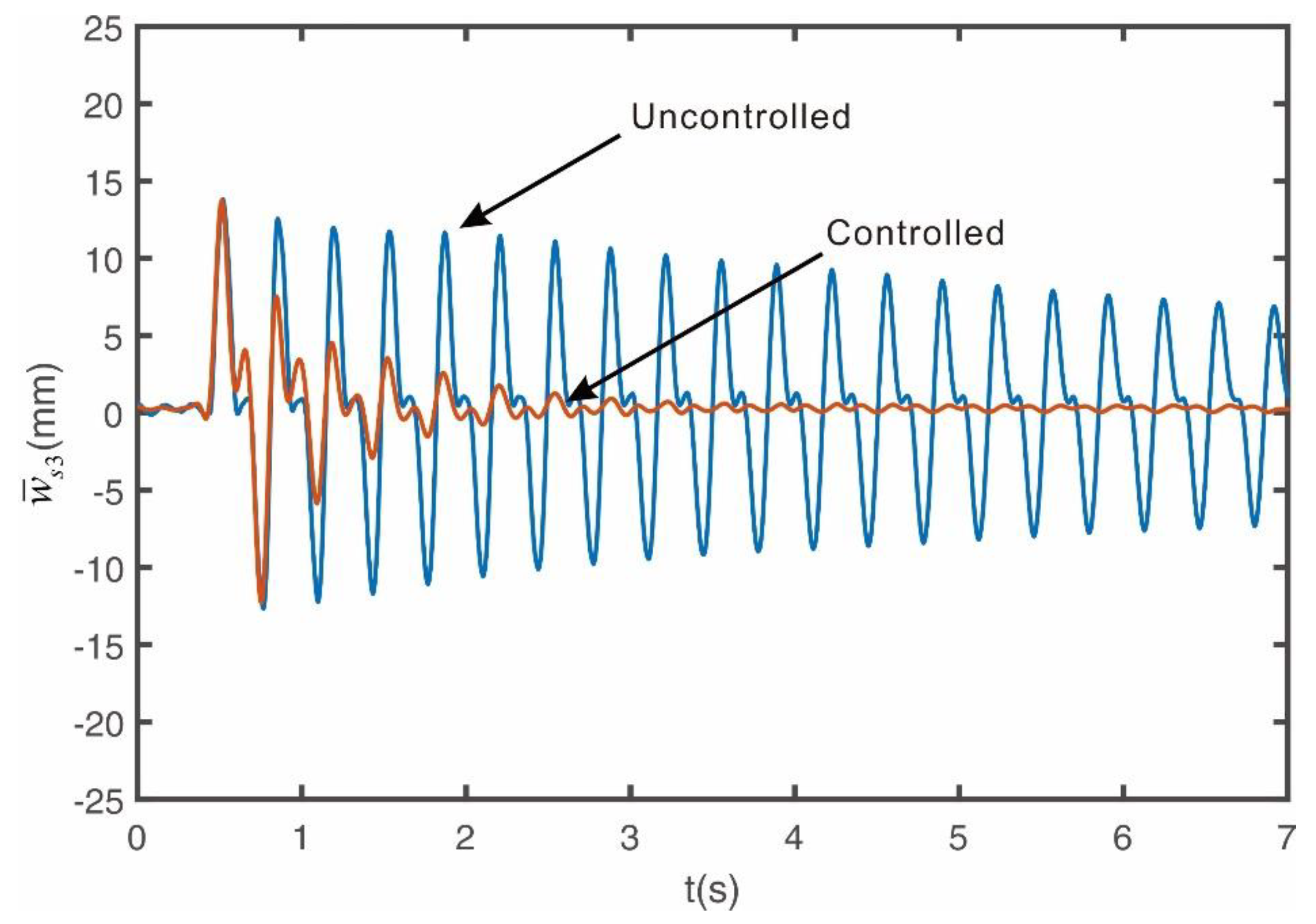
Figure 10.
Experimental free vibration response with the first mode excited.
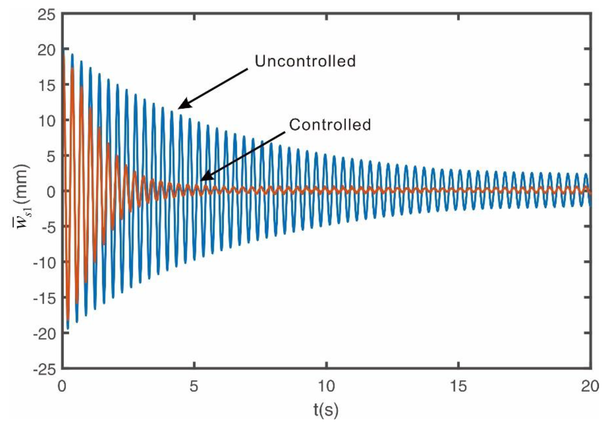
Figure 11.
Experimental free vibration response with the second mode excited.
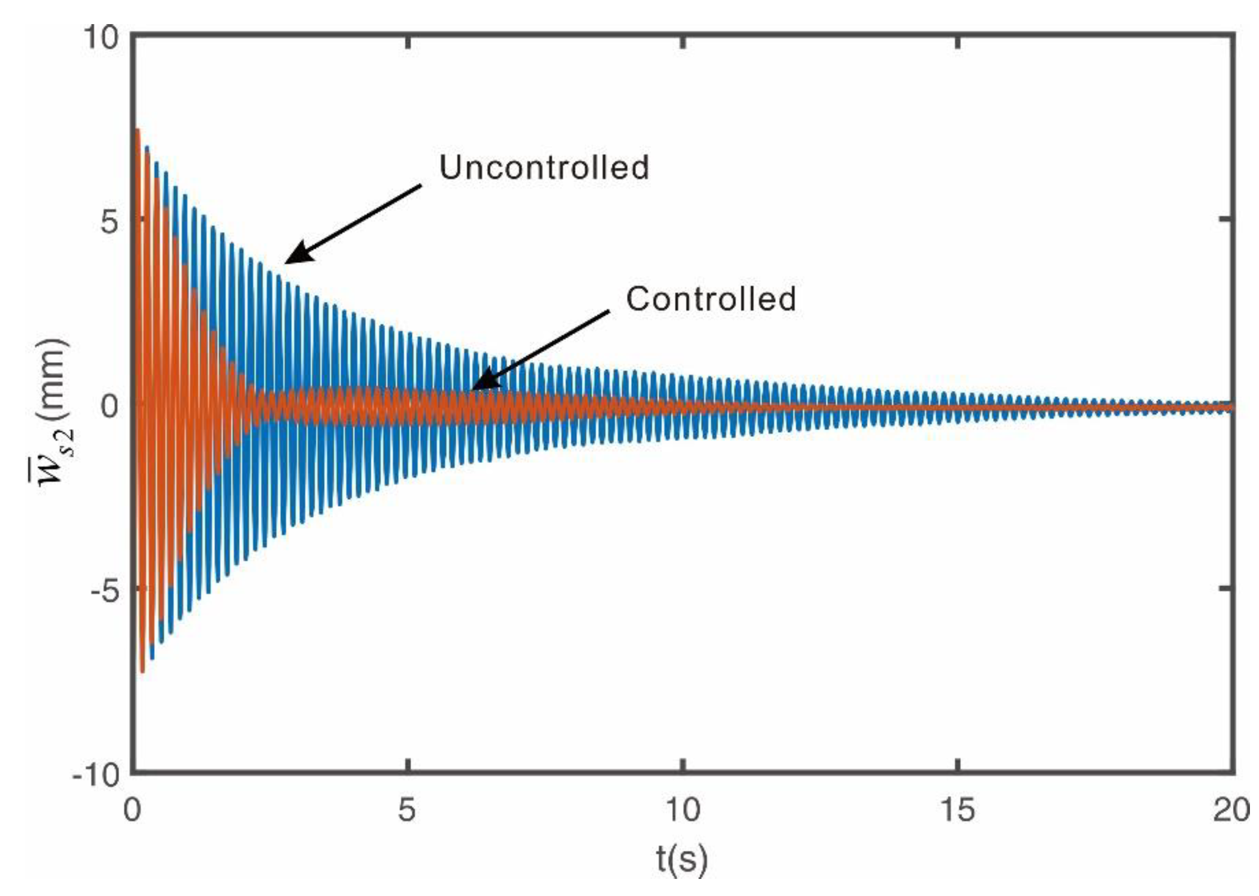
Figure 12.
Experimental free vibration response with the third mode excited.
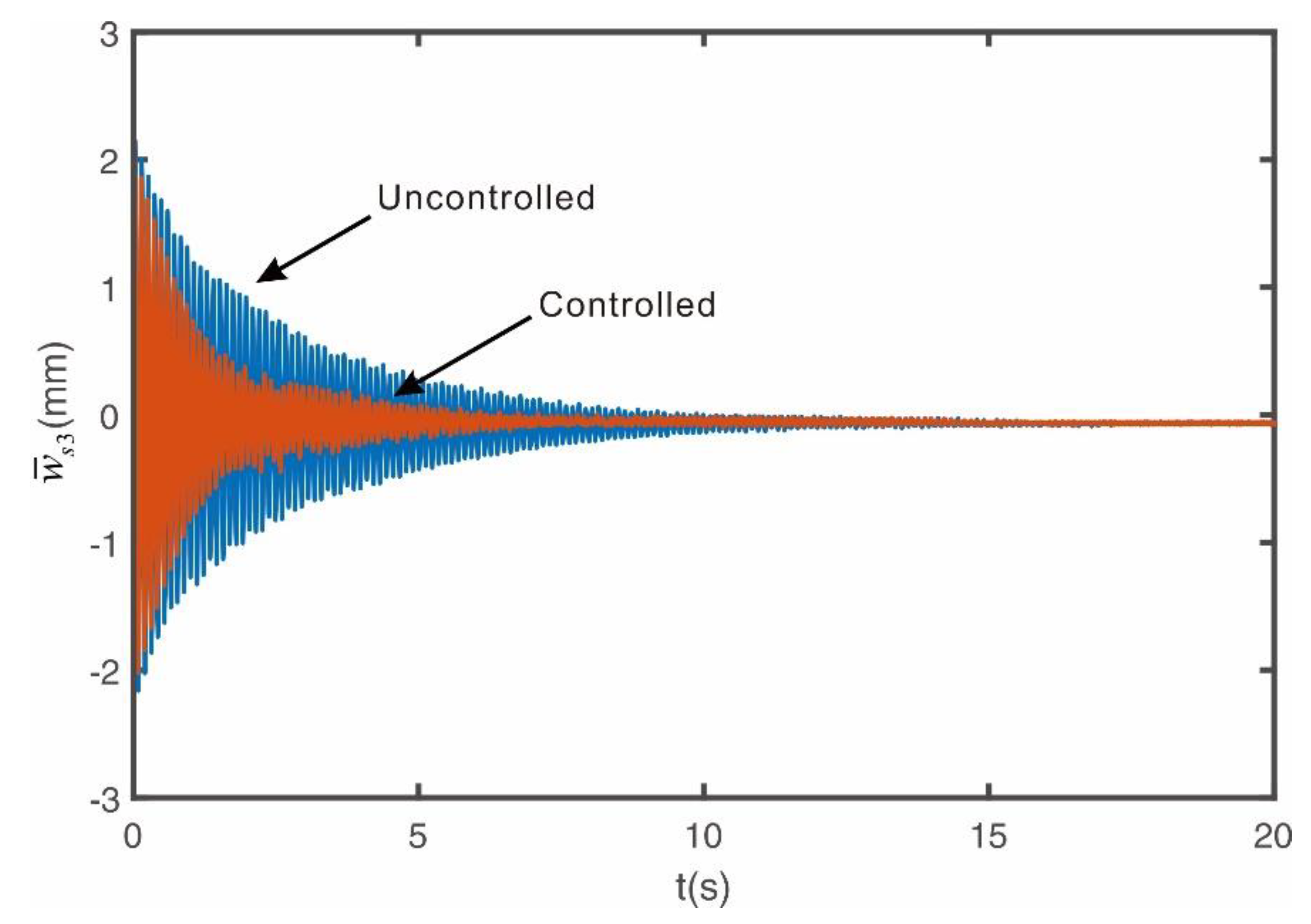

Table 1.
Parameters and material properties of string for numerical analysis.
| Mass per unit length | ||
| Length | ||
| Tension | ||
| Damping ratio | 0.006 | |
| Number of admissible functions | 10 | |
| Number of modes to be controlled | 3 | |
| Compensator damping factor | 0.3 | |
| Controller gain matrix | ||
| FRF measurement point | 0.12 |
Disclaimer/Publisher’s Note: The statements, opinions and data contained in all publications are solely those of the individual author(s) and contributor(s) and not of MDPI and/or the editor(s). MDPI and/or the editor(s) disclaim responsibility for any injury to people or property resulting from any ideas, methods, instructions or products referred to in the content. |
© 2025 by the authors. Licensee MDPI, Basel, Switzerland. This article is an open access article distributed under the terms and conditions of the Creative Commons Attribution (CC BY) license (http://creativecommons.org/licenses/by/4.0/).
Copyright: This open access article is published under a Creative Commons CC BY 4.0 license, which permit the free download, distribution, and reuse, provided that the author and preprint are cited in any reuse.


