Cost-Benefit Analysis of Environmental Projects: An Integrated Theoretical Framework

1. Introduction

The increasing awareness of environmental degradation and climate change has led to a surge in environmental projects aimed at mitigating these issues. These projects, ranging from renewable energy initiatives to conservation efforts, are crucial in addressing the pressing challenges of our time (Stern, 2007; IPCC, 2022). However, the success of these projects hinges on their ability to deliver tangible benefits that outweigh the costs involved. Cost-benefit analysis (CBA) is a crucial tool in evaluating the economic feasibility and overall impact of such projects, yet its application to environmental contexts remains problematic (Arrow et al., 2013).

The theoretical foundations of CBA are deeply rooted in welfare economics and public finance. Since its formalization by Dupuit in the 19th century and subsequent development by Kaldor (1939), Hicks (1939), and others, CBA has become the predominant framework for evaluating public investments. At its core, CBA involves comparing the total expected benefits of a project with its total expected costs, both expressed in monetary terms. The primary objective is to determine whether the project is worth undertaking from an economic perspective by evaluating whether the present value of benefits exceeds the present value of costs (Boardman et al., 2017).

However, when applied to environmental contexts, traditional CBA encounters several theoretical and methodological challenges that limit its effectiveness. First, environmental projects often generate benefits that extend far into the future, raising questions about appropriate discount rates and intergenerational equity (Goulder & Williams, 2012). The choice of discount rate is not merely a technical matter but embodies profound ethical judgments about the relative importance of present versus future generations (Dasgupta, 2008). Stern (2007) advocated for near-zero discount rates for climate change mitigation projects, while others like Nordhaus (2007) argued for rates closer to market returns, illustrating the contentious nature of this parameter.

Second, environmental projects generate numerous non-market benefits that are challenging to quantify in monetary terms (Costanza et al., 2014). These include improvements in biodiversity, ecosystem services, air and water quality, and human health and well-being. While economic theory has developed various methods for non-market valuation, including contingent valuation, choice experiments, hedonic pricing, and travel cost methods, each approach has limitations and uncertainties (Carson, 2012; Bateman et al., 2011). The resulting estimates can vary widely depending on the methodology, context, and population surveyed, raising questions about their reliability and validity.

Third, environmental projects often involve significant uncertainties and risks that are difficult to incorporate into traditional CBA frameworks (Heal & Millner, 2014). Climate change, for instance, involves deep uncertainties about future emissions trajectories, climate sensitivity, and potential tipping points. Biodiversity conservation projects may face uncertainties about species responses to management interventions, ecosystem dynamics, and future threats. These uncertainties call for more sophisticated approaches that go beyond deterministic benefit-cost calculations to incorporate probabilistic reasoning and robust decision-making under uncertainty (Polasky et al., 2011).

Fourth, environmental projects typically generate impacts across multiple dimensions (Montgomery, 2024), including economic, environmental, and social domains (de Groot et al., 2010). Traditional CBA tends to focus primarily on economic efficiency, potentially neglecting important ecological and social considerations. This narrow focus can lead to decisions that maximize economic returns at the expense of environmental sustainability or social equity (Howarth & Norgaard, 2013). Moreover, the attempt to reduce all values to a single monetary metric has been criticized as reductionist and potentially obscuring important value dimensions that resist monetization (Spash, 2008; Vatn, 2009).

These limitations have prompted various extensions and alternatives to traditional CBA, including multi-criteria analysis (Belton & Stewart, 2002), deliberative valuation (Wilson & Howarth, 2002), and integrated assessment modeling (Weyant, 2017). While these approaches offer valuable insights, they often lack a unified theoretical framework that can systematically integrate economic, environmental, and social dimensions within a coherent decision-making structure. As Farrow (2004) observes, “The challenge is not to abandon benefit-cost analysis but to improve it and complement it with other approaches that can address its limitations” (p. 47).

Furthermore, the application of CBA to environmental projects has been critiqued from various philosophical perspectives. Ecological economists argue that CBA’s assumption of weak sustainability (where natural and manufactured capital are substitutable) is fundamentally flawed and that strong sustainability principles should guide environmental decision-making (Daly, 2007). Environmental ethicists question the anthropocentric orientation of CBA and argue for recognizing the intrinsic value of nature beyond its instrumental value to humans (O’Neill et al., 2008). Critical theorists suggest that CBA’s technocratic approach can mask power dynamics and reinforce existing inequalities in environmental decision-making (Forsyth, 2003).

Despite these critiques, CBA remains a dominant framework in environmental policy and project evaluation due to its theoretical grounding in welfare economics, its ability to provide clear decision rules, and its alignment with budgetary and fiscal processes (Pearce et al., 2006; Sunstein, 2018). Rather than abandoning CBA, many scholars have called for its refinement and extension to better address environmental complexities (Atkinson & Mourato, 2008; Barbier, 2011). As Gowdy et al. (2010) note, “Economics has much to offer to environmental decision-making, but only if it moves beyond simplistic applications of standard theory” (p. 35).

This paper addresses these challenges by proposing a theoretical framework that integrates environmental and social factors alongside economic considerations in a unified mathematical structure. The model is designed to provide a holistic assessment of environmental projects, enabling decision-makers to make more informed and balanced judgments. By explicitly recognizing multiple value dimensions, incorporating temporal dynamics, and addressing uncertainty, the framework aims to overcome the limitations of traditional CBA while retaining its analytical rigor and decision-making utility.

1.1. Theoretical Background

Our framework builds on three foundational areas in economics and decision theory:

• Welfare Economics: The theoretical basis for cost-benefit analysis rests on the principles of welfare economics, particularly the Kaldor-Hicks compensation criterion, which states that a project is desirable if those who gain could potentially compensate those who lose, with a net positive outcome (Just et al., 2004). We extend this to include intergenerational equity considerations especially relevant to environmental projects.
• Environmental Valuation Theory: The economic valuation of environmental goods and services draws upon theories of total economic value (TEV), which encompasses use values (direct, indirect, and option values) and non-use values (existence and bequest values) (Pearce et al., 2006).
• Multi-Criteria Decision Analysis (MCDA): When multiple, potentially conflicting objectives exist, MCDA provides theoretical frameworks for structuring complex problems, incorporating diverse stakeholder perspectives, and making trade-offs explicit (Belton & Stewart, 2002).

1.2. Research Gap and Contribution

While extensive literature exists on both CBA and environmental economics, there remains a theoretical gap in frameworks that simultaneously:

• Integrate economic, environmental, and social dimensions in a coherent mathematical structure
• Address temporal dynamics across all dimensions
• Account for uncertainty and risk in a unified way
• Provide clear methodological guidance for non-market valuation within CBA
• This paper contributes to the literature by proposing a theoretical framework that addresses these gaps, thereby enhancing the applicability of CBA to complex environmental projects.

2. Methodology

The methodology section presents the mathematical equations used in the model, along with a progressive explanation of the variables involved.

The economic evaluation follows standard cost-benefit analysis (CBA). The three primary measures are:

• Net Present Value (NPV) The NPV of a project is defined as the present value of net benefits:

  $$\mathrm{N}\mathrm{P}\mathrm{V}={\sum }_{t=0}^T {\displaystyle \frac{B_t-C_t}{(1+r{)}^t}}$$

  (1)

  where:
  • $B_t$ is the benefit at time $t$,
  • $C_t$ is the cost at time $t$,
  • $r$ is the discount rate, and
  • $T$ is the time horizon.
• Internal Rate of Return (IRR)
  The IRR is the discount rate that satisfies:

  $${\sum }_{t=0}^T {\displaystyle \frac{B_t-C_t}{(1+\mathrm{I}\mathrm{R}\mathrm{R}{)}^t}}=0$$

  (2)
• Benefit-Cost Ratio (BCR)
  The BCR is given by:

  $$\mathrm{B}\mathrm{C}\mathrm{R}={\displaystyle \frac{{\sum }_{t=0}^T \frac{B_t}{(1+r{)}^t}}{{\sum }_{t=0}^T \frac{C_t}{(1+r{)}^t}}}$$

  (3)

For convenience in the integrated framework, we define the net economic contribution at time $t$ as:

$$EC\left(t\right)=B_t-C_t$$

(4)

2.1. Environmental Dimension

Environmental impacts are assessed through a set of indicators that capture different ecological aspects:

2.2. Carbon Impact Function

The net carbon impact is modeled as:

$$CI\left(t\right)=E_b-E\left(t\right)$$

(5)

where:

• $E_b$ is the baseline emissions, and
• $E\left(t\right)$ is the emissions with the project at time $t$.

2.

Biodiversity Conservation Function

Biodiversity value is expressed as:

$$BD\left(t\right)=\alpha S\left(t\right)+\beta H\left(t\right)+\gamma G\left(t\right)$$

(6)

where:

• $S\left(t\right)$ is the species richness index,
• $H\left(t\right)$ is the habitat quality index,
• $G\left(t\right)$ is the genetic diversity index, and
• $\alpha ,\beta ,\gamma$ are weighting parameters reflecting ecological significance.

3.

Environmental Quality Function

A composite quality indicator is given by:

$$EQ\left(t\right)={\sum }_{i=1}^n w_i{q}_i\left(t\right)$$

(7)

where:

• $q_i\left(t\right)$ is the quality index for environmental component $i$ at time $t$,
• $w_i$ is the weight for component $i$, and
• $n$ is the number of environmental components.

Combining these, we represent the total environmental value as:

$$ENV\left(t\right)={\omega }_{C}CI\left(t\right)+{\omega }_{B}BD\left(t\right)+{\omega }_{E}EQ\left(t\right)$$

(8)

Substituting equations (5), (6), and (7) gives:

$$ENV\left(t\right)={\omega }_C\left[E_b-E\left(t\right)\right]+{\omega }_B\left[\alpha S\right(t)+\beta H(t)+\gamma G(t\left)\right]+{\omega }_E\left[{\sum }_{i=1}^n w_i{q}_i\left(t\right)\right]$$

(9)

where ${\omega }_C,{\omega }_B$, and ${\omega }_E$ are conversion factors that translate environmental impacts into monetary units.

2.3. Social Dimension

The social impact is captured by aggregating multiple social indicators:

• Social Welfare Function
  The basic social welfare is:

  $$SW\left(t\right)={\sum }_{j=1}^m {\lambda }_j{s}_j\left(t\right)$$

  (10)

  where:
  • $s_j\left(t\right)$ is social indicator $j$ at time $t$,
  • ${\lambda }_j$ is the weight for indicator $j$, and
  • $m$ is the number of social indicators.
• Employment Function
  Employment benefits are modeled as:

  $$EMP\left(t\right)=J_d\left(t\right)+\delta J_i\left(t\right)$$

  (10)

  where:
  • $J_d\left(t\right)$ is the number of direct jobs created at time $t$,
  where:
  • $J_d\left(t\right)$ is the number of direct jobs created at time $t$,
  • $J_i\left(t\right)$ is the number of indirect jobs, and
  • $\delta$ reflects the relative economic weight of indirect jobs.
• Health Impact Function
  Health outcomes are expressed as:

  $$HI\left(t\right)={\sum }_{k=1}^p {\mu }_k{h}_k\left(t\right)$$

  (12)

  where:
  • $h_k\left(t\right)$ is health indicator $k$ at time $t$,
  • ${\mu }_k$ is the corresponding weight, and
  • $p$ is the number of health indicators.

The overall social value is then given by:

$$SOC\left(t\right)={\lambda }_{W}SW\left(t\right)+{\lambda }_{E}EMP\left(t\right)+{\lambda }_{H}HI\left(t\right)$$

or, equivalently,

$$SOC\left(t\right)={\lambda }_W\left[{\sum }_{j=1}^m {\lambda }_j{s}_j\left(t\right)\right]+{\lambda }_E\left[J_d\left(t\right)+\delta J_i\left(t\right)\right]+{\lambda }_H\left[{\sum }_{k=1}^p {\mu }_k{h}_k\left(t\right)\right]$$

(13)

where ${\lambda }_W,{\lambda }_E$, and ${\lambda }_H$ are conversion factors to monetary terms.

2.4. Integrated Value Function

The core of the framework is the integrated value (IV), which aggregates economic, environmental, and social values over time. It is defined as:

$$IV={\int }_0^T \left[EC\right(t)+\varphi ENV(t)+\psi SOC(t\left)\right]e^{-rt}dt$$

(14)

where:

• $\varphi$ and $\psi$ are conversion factors for environmental and social values, respectively,
• $e^{-rt}$ is the discounting term using the social discount rate $r$,
• $T$ is the project’s time horizon.

A project is deemed acceptable if $IV>0$, and when comparing alternatives (e.g., project A vs. project B), the decision rule is:

$$I{V}_A>I{V}_B$$

(14)

2.5. Addressing Temporal Dynamics

Given the long-term impacts typical of environmental projects, a time-varying (or declining) discount rate is adopted. One proposed form is:

$$r\left(t\right)=r_0{e}^{-\eta ,t}$$

(15)

where:

• $r_0$ is the initial discount rate,
• $\eta$ is a decline parameter that accounts for increased uncertainty over time.

Alternatively, following a derivation based on uncertainty in the discount rate (assuming a gamma distribution for $r$), the effective discount rate can be expressed as:

$$r\left(t\right)={\displaystyle \frac{a}{b+t}}$$

(16)

with parameters $a$ and $b$ determined by the underlying probability distribution.

2.6. Incorporating Uncertainty and Risk

Environmental projects face deep uncertainties. To account for these, the framework introduces a probabilistic approach and a risk adjustment:

• Expected Integrated Value
  The expected value over all states $\omega$ in the uncertainty set $\mathsf{\Omega }$ is:

  $$E\left[IV\right]={\int }_{\mathsf{\Omega }} IV\left(\omega \right)p\left(\omega \right)d\omega$$

  (17)
  For computational purposes, this may be discretized as:

  $$E\left[IV\right]\approx {\sum }_{i=1}^N IV\left({\omega }_i\right)p\left({\omega }_i\right)$$

  (18)
• Risk Adjustment
  To incorporate risk aversion, a risk-adjusted integrated value is defined as:

  $$I{V}_{\mathrm{risk}}=E\left[IV\right]-\lambda \mathrm{V}\mathrm{a}\mathrm{r}\left[IV\right]$$

  (19)

  where the variance is:

  $$\mathrm{V}\mathrm{a}\mathrm{r}\left[IV\right]={\int }_{\mathsf{\Omega }} \left(IV\right(\omega )-E[IV\left]{)}^{2}p\right(\omega )d\omega$$

  (20)

  and $\lambda$ is the risk aversion coefficient.
• Robust Decision Making
  For cases of deep uncertainty (where probabilities are not well defined), the maximin criterion can be used:

  $$\underset{a\in A}{\mathrm{m}\mathrm{a}\mathrm{x}} \underset{\omega \in {\mathsf{\Omega }}^{\prime }}{\mathrm{m}\mathrm{i}\mathrm{n}} IV(a,\omega )$$

  (21)

  where $A$ represents the set of decision alternatives and ${\mathsf{\Omega }}^{\prime }$ a set of plausible future states.

2.7. Sensitivity Analysis

To explore the sensitivity of the integrated value to the conversion factors $\varphi$ and $\psi$, we compute the partial derivatives:

• Sensitivity with respect to $\varphi$:

  $${\displaystyle \frac{\partial IV}{\partial \varphi }}={\int }_0^T ENV\left(t\right)e^{-rt}dt$$

  (22)
• Sensitivity with respect to $\psi$

  $${\displaystyle \frac{\partial IV}{\partial \psi }}={\int }_0^T SOC\left(t\right)e^{-rt}dt$$

  (23)
  The ratio of these sensitivities,

  $${\displaystyle \frac{\frac{\partial IV}{\partial \varphi }}{\frac{\partial IV}{\partial \psi }}}={\displaystyle \frac{{\int }_0^T ENV\left(t\right)e^{-rt}dt}{{\int }_0^T SOC\left(t\right)e^{-rt}dt}}$$

  (24)

provides insight into the relative importance of environmental versus social impacts in the overall project assessment.

8. Detailed Mathematical Derivations

For completeness, we now integrate the derivations from the appendix into our methodological discussion.

2.8. Derivation of the Integrated Value Function

Starting with the definition:

$$IV={\int }_0^T \left[EC\right(t)+\varphi ENV(t)+\psi SOC(t\left)\right]e^{-rt}dt$$

(25)

we substitute:

• $EC\left(t\right)=B_t-C_t($ from (4)),
• $ENV\left(t\right)$ from (8a), and
• $\mathrm{S}\mathrm{O}\mathrm{C}\left(t\right)$ from (12a).

This yields an expanded form:

$$\begin{array}{l}IV={\int }_0^T\{\left[B_t-C_t\right]\\ \hspace{1em}\hspace{1em}\hspace{1em}\hspace{1em}+\varphi \left({\omega }_C\left[E_b-E\left(t\right)\right]+{\omega }_B\left[\alpha S\right(t)+\beta H(t)+\gamma G(t\left)\right]+{\omega }_E{\displaystyle \sum _{i=1}^n} w_i{q}_i\left(t\right)\right)\\ \hspace{1em}\hspace{1em}\hspace{1em}\hspace{1em}\left.+\psi \left({\lambda }_W{\displaystyle \sum _{j=1}^m} {\lambda }_j{s}_j\left(t\right)+{\lambda }_E\left[J_d\left(t\right)+\delta J_i\left(t\right)\right]+{\lambda }_H{\displaystyle \sum _{k=1}^p} {\mu }_k{h}_k\left(t\right)\right)\right\}{e}^{-rt}dt.\end{array}$$

(26)

2.9. Optimal Decision Rule

For a project to be acceptable, the integrated value must be positive:

$$IV>0$$

(27)

When comparing two projects (A and B), the decision criterion is:

$$I{V}_A>I{V}_B$$

(28)

2.10. Time-Declining Discount Rate Derivation

Assume that the discount rate $r$ is a random variable with density $f\left(r\right)$. The present value of a benefit

$B$ at time $t$ is:

$$PV(B,t)=BE\left[e^{-rt}\right]=B{\int }_0^{\mathrm{\infty }} e^{-rt}f\left(r\right)dr$$

(29)

This can be written as:

$$PV(B,t)=B{e}^{-r\left(t\right)t}$$

(30)

where the effective discount rate $r\left(t\right)$ is defined by:

$$r\left(t\right)=-{\displaystyle \frac{1}{t}}\ln \left({\int }_0^{\mathrm{\infty }} e^{-rt}f\left(r\right)dr\right)$$

(31)

For a gamma distribution with parameters $a$ and $b$, this simplifies to:

$$r\left(t\right)={\displaystyle \frac{a}{b+t}}$$

(32)

2.11. Risk-Adjusted Integrated Value

To incorporate risk, a risk-adjustment factor $\theta \left(t\right)$ is introduced:

$$I{V}_{\mathrm{risk}}={\int }_0^T \left[EC\left(t\right)+\varphi ENV\left(t\right)+\psi SOC\left(t\right)\right]\theta \left(t\right)e^{-rt}dt$$

(33)

with

$$\theta \left(t\right)={\displaystyle \frac{1}{1+\rho \sigma \left(t\right)}}$$

(34)

where:

• $\rho$ is the risk aversion coefficient,
• $\sigma \left(t\right)$ is the standard deviation of outcomes at time $t$.

For numerical evaluation, the integral (30) may be discretized as:

$$I{V}_{\mathrm{risk}}\approx {\sum }_{t=0}^T \left[EC\right(t)+\varphi ENV(t)+\psi SOC(t\left)\right]\theta \left(t\right)e^{-rt}\mathsf{\Delta }t$$

(35)

2.12. Sensitivity Analysis of Conversion Factors

The responsiveness of the integrated value to changes in the environmental conversion factor $\varphi$ and the social conversion factor $\psi$ is given by:

$${\displaystyle \frac{\partial IV}{\partial \varphi }}={\int }_0^T ENV\left(t\right)e^{-rt}dt$$

(36)

$$\begin{array}{rr}& \\ & {\displaystyle \frac{\partial IV}{\partial \psi }}={\int }_0^T SOC\left(t\right)e^{-rt}dt\end{array}$$

(37)

The ratio,

$${\displaystyle \frac{\frac{\partial IV}{\partial \varphi }}{\frac{\partial IV}{\partial \psi }}}={\displaystyle \frac{{\int }_0^T ENV\left(t\right)e^{-rt}dt}{{\int }_0^T SOC\left(t\right)e^{-rt}dt}}$$

(38)

indicates whether the integrated value is more sensitive to environmental or social impacts.

• Summary

This integrated framework systematically combines economic, environmental, and social impacts into a single valuation measure, addressing long-term dynamics and uncertainty through time-varying discount rates and risk adjustments. Equations (1)-(39) provide a formal, step-by-step explanation of the methodology, ensuring transparency in assumptions and variable definitions.

This revised and numbered presentation of the mathematical derivations (originally in the appendix) is now embedded within the methodology, thereby creating a cohesive and comprehensive framework for the cost-benefit analysis of environmental projects.

3. Results

Figure 1. Economic, Environmental and Social Dimensions.

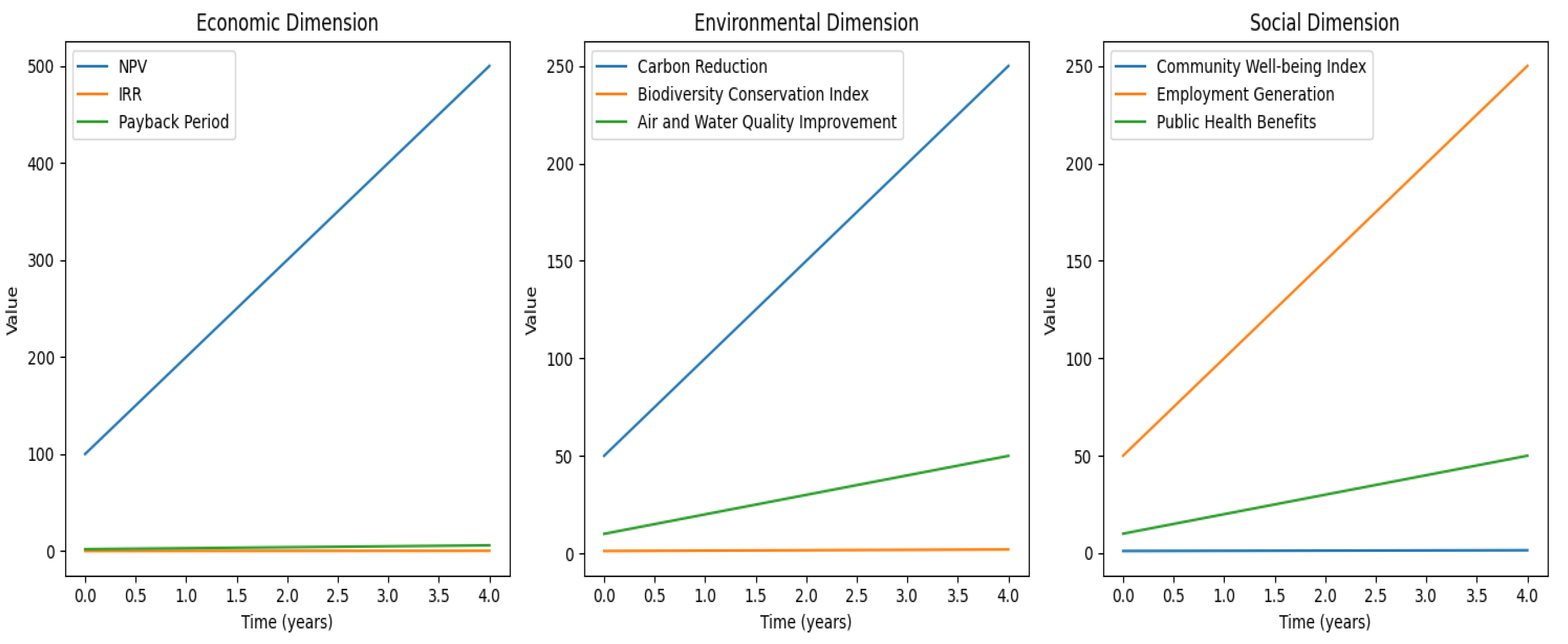
Figure 1. Economic, Environmental and Social Dimensions.

Explanations

• Economic Dimension Graph: This graph shows how the financial aspects of the project change over time. The Net Present Value (NPV) represents the difference between the project’s benefits and costs, adjusted for the time value of money. A positive NPV indicates that the project is profitable. The Internal Rate of Return (IRR) is the discount rate at which the NPV is zero, providing a measure of the project’s profitability. The Payback Period is the time it takes to recover the initial investment. A shorter payback period is generally preferred.
• Environmental Dimension Graph: This graph illustrates the project’s environmental impacts over time. Carbon Reduction shows the decrease in greenhouse gas emissions due to the project. The Biodiversity Conservation Index measures the project’s contribution to preserving local ecosystems and species (Montgomery, 2024a). The Air and Water Quality Improvement index reflects enhancements in air and water quality resulting from the project.
• Social Dimension Graph: This graph demonstrates the project’s social impacts over time. The Community Well-being Index measures improvements in the quality of life for local residents. Employment Generation shows the number of jobs created or supported by the project. Public Health Benefits reflect health improvements resulting from the project, such as reduced respiratory diseases.

These graphs provide a visual representation of the project’s impacts across economic, environmental, and social dimensions, helping decision-makers understand the comprehensive benefits of the project.

Figure 2. Sensitivity Surface of Integrated Value.

Figure 2. Sensitivity Surface of Integrated Value.

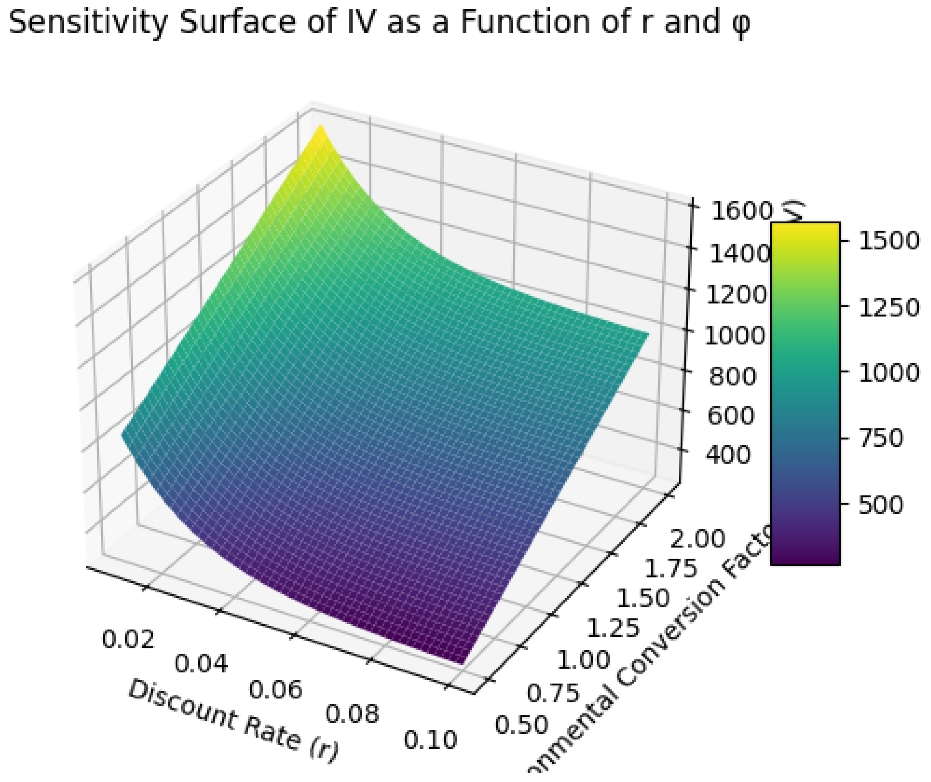
Explanation:

This 3D surface plot shows how the overall integrated value (IV) of a project changes as a function of two critical parameters: the discount rate (r) and the environmental conversion factor (ϕ). In this synthetic example, the IV is modeled as a combination of a discounted economic component and a scaled environmental benefit. The plot highlights the sensitivity of the overall valuation to these parameters, illustrating that a higher discount rate (implying greater impatience or uncertainty) significantly reduces the economic contribution, while a higher environmental conversion factor increases the overall IV. This graph underscores the importance of choosing appropriate values for these parameters in the decision-making process.

Figure 3. Temporal Dynamics of Project Values.

Figure 3. Temporal Dynamics of Project Values.

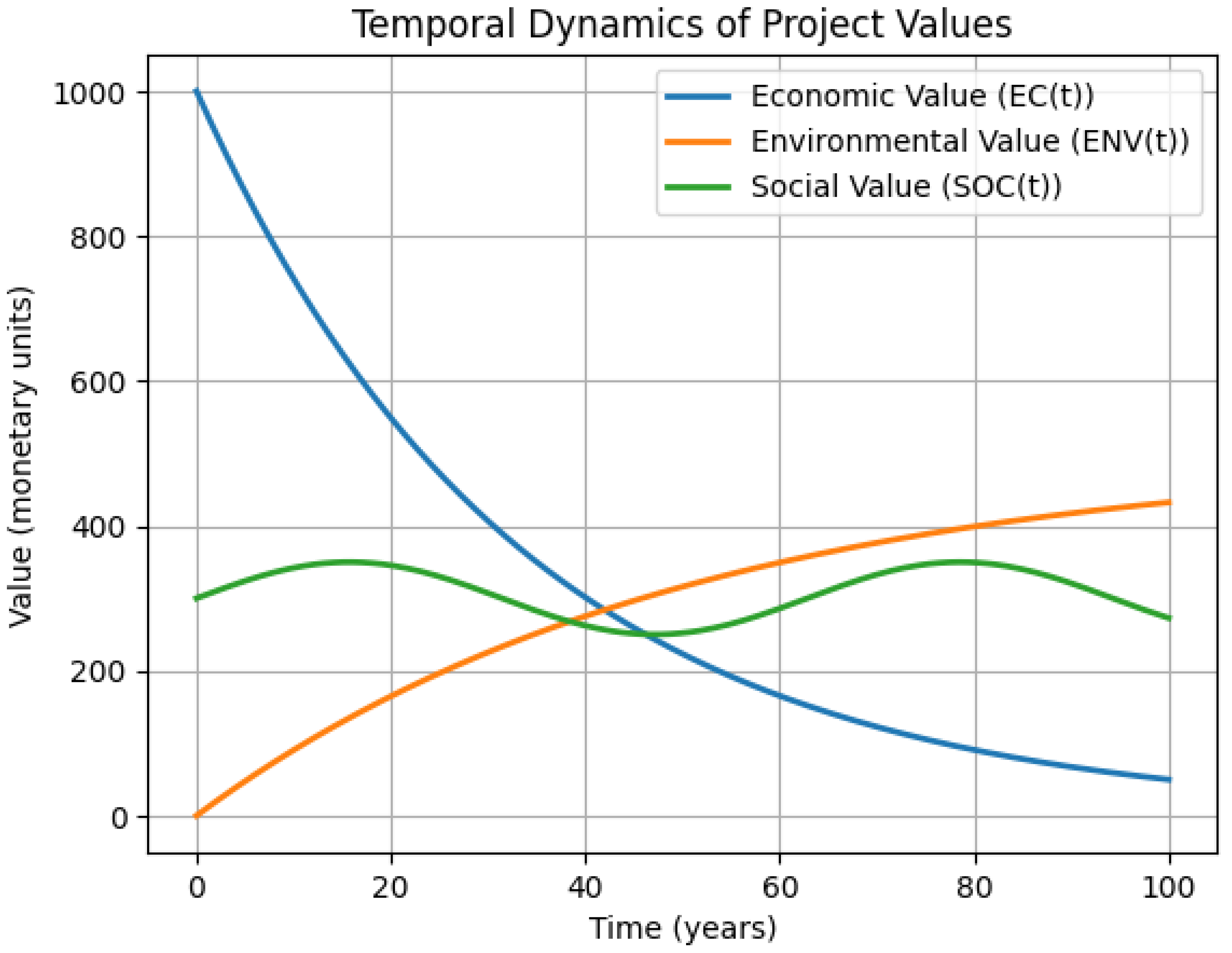
Explanation:

This time-series plot depicts the evolution of the three core dimensions—economic EC(t), environmental ENV(t), and social SOC(t) values—over the project’s lifetime. In this example, the economic value declines over time due to discounting effects and potential project depreciation. In contrast, the environmental benefit accumulates gradually, reflecting long-term ecological improvements, while the social value fluctuates as community impacts evolve. The graph illustrates how benefits from each dimension accrue at different rates and underscores the need to consider all dimensions over time when evaluating environmental projects.

Figure 4. Impact of Risk Aversion on Valuation.

Figure 4. Impact of Risk Aversion on Valuation.

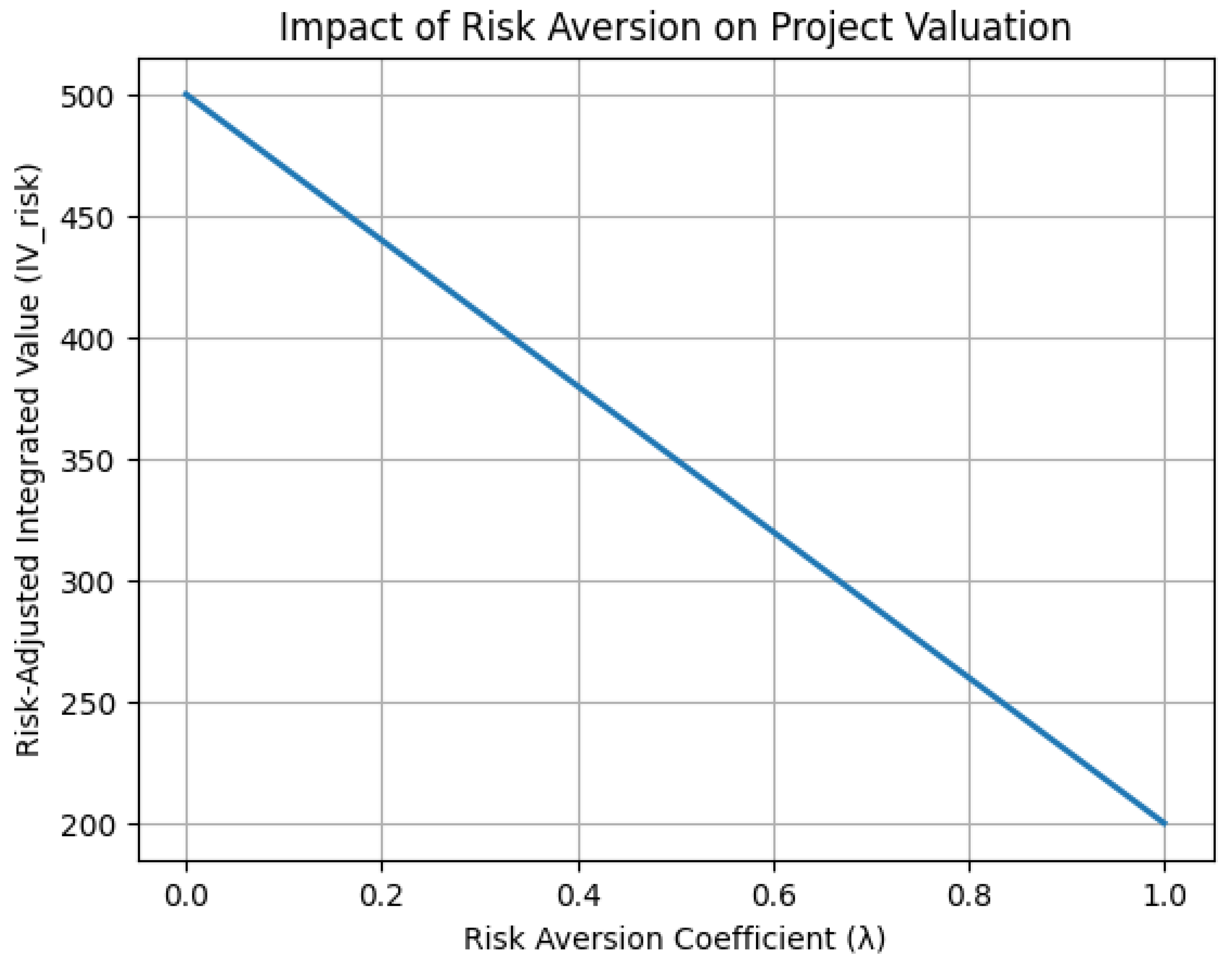
Explanation:

This graph illustrates the effect of risk aversion on the risk-adjusted integrated value IVrisk of a project. The horizontal axis represents the risk aversion coefficient λ, while the vertical axis shows the corresponding IVrisk . In this example, a higher risk aversion leads to a lower adjusted value because the decision-maker discounts the expected integrated value by an amount proportional to the outcome variance. The graph provides insight into how risk attitudes can alter project evaluations, emphasizing that robust decision-making must account for risk in addition to mean benefits.

Figure 5. Comparison of Evaluation Methods.

Figure 5. Comparison of Evaluation Methods.

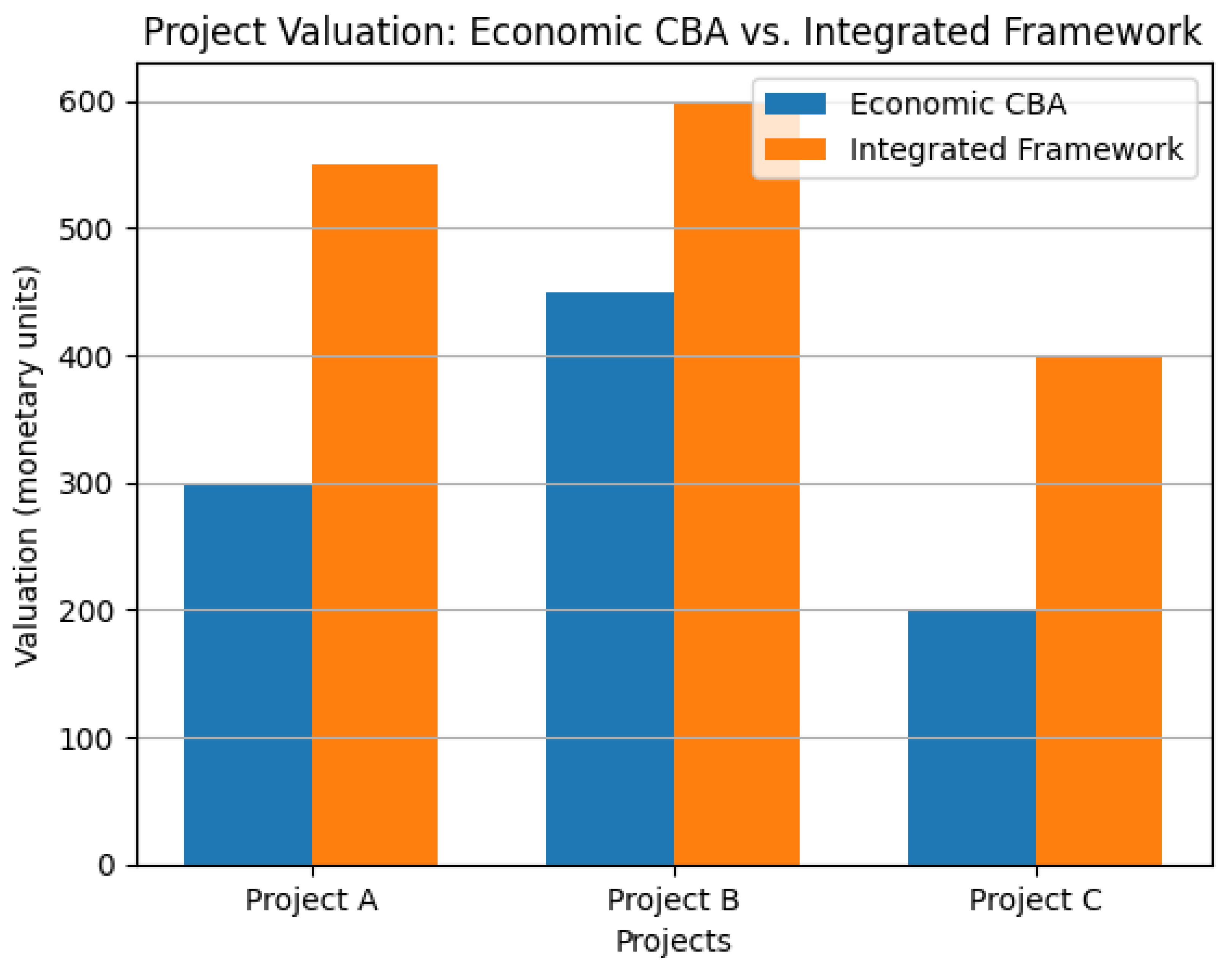
Explanation:

This bar chart compares project valuations derived from a traditional economic cost–benefit analysis (which considers only the economic dimension) versus the integrated framework (which also includes environmental and social impacts). Three hypothetical projects are evaluated. For each project, two bars represent the outcomes from the economic-only approach and the integrated framework. Notice that the integrated approach typically yields a higher valuation, as it captures additional benefits that are not reflected in a narrow economic analysis. This comparison clearly demonstrates the potential for misallocation of resources if environmental and social factors are omitted from the evaluation.

Figure 6. Sensitivity of Integrated Value to Environmental and Social Conversion Factors.

Figure 6. Sensitivity of Integrated Value to Environmental and Social Conversion Factors.

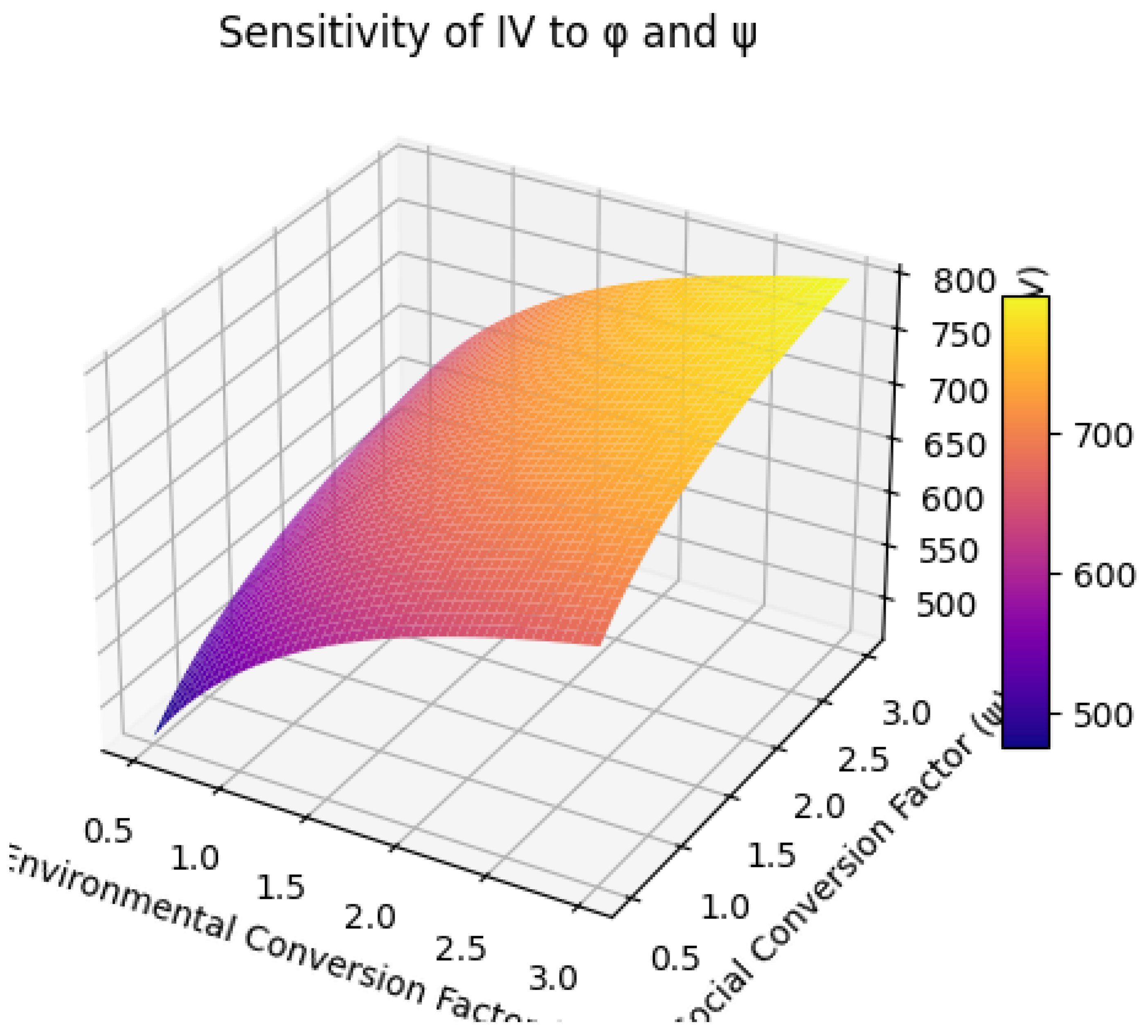
Explanation:

This 3D surface plot explores how the overall integrated value (IV) changes as a function of both the environmental conversion factor (ϕ) and the social conversion factor (ψ). In the integrated framework, these conversion factors translate non-market environmental and social benefits into monetary terms. The graph uses a non-linear synthetic function to mimic diminishing returns in both dimensions. It demonstrates that as either ϕ or ψ increases, the integrated value increases—but at a decreasing rate. This visualization helps decision makers understand the importance and interplay of these two factors when aggregating benefits.

Graph 7. This multi-line plot illustrates how the integrated value (IV) evolves over time for three different discount rates. For each discount rate, the graph shows the cumulative effect of economic, environmental, and social benefits over a project’s lifetime. The economic component declines over time due to discounting, while environmental and social benefits accumulate gradually. By comparing curves for discount rates r=0.02, 0.050, and 0.080, the graph emphasizes how higher discount rates reduce the present value of long-term benefits—a key consideration when planning sustainable projects.

Graph 7. This multi-line plot illustrates how the integrated value (IV) evolves over time for three different discount rates. For each discount rate, the graph shows the cumulative effect of economic, environmental, and social benefits over a project’s lifetime. The economic component declines over time due to discounting, while environmental and social benefits accumulate gradually. By comparing curves for discount rates r=0.02, 0.050, and 0.080, the graph emphasizes how higher discount rates reduce the present value of long-term benefits—a key consideration when planning sustainable projects.

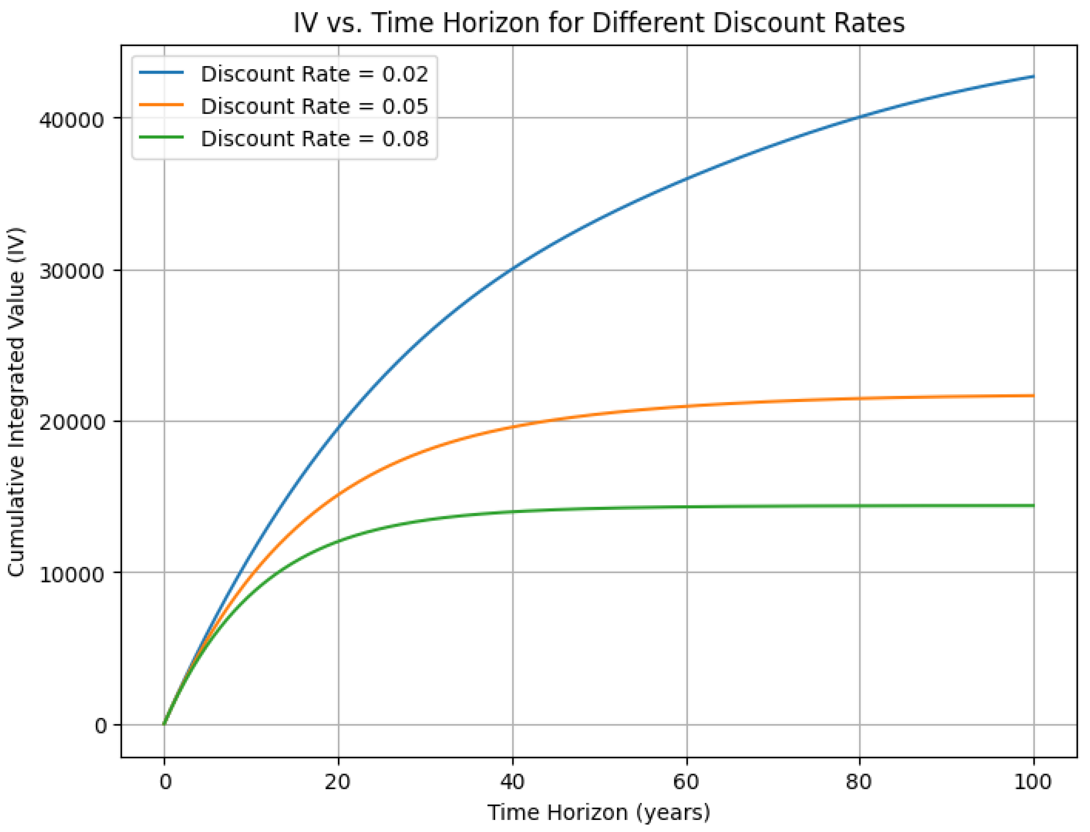
Figure 8. Monte Carlo Simulation of Integrated Value Distribution.

Figure 8. Monte Carlo Simulation of Integrated Value Distribution.

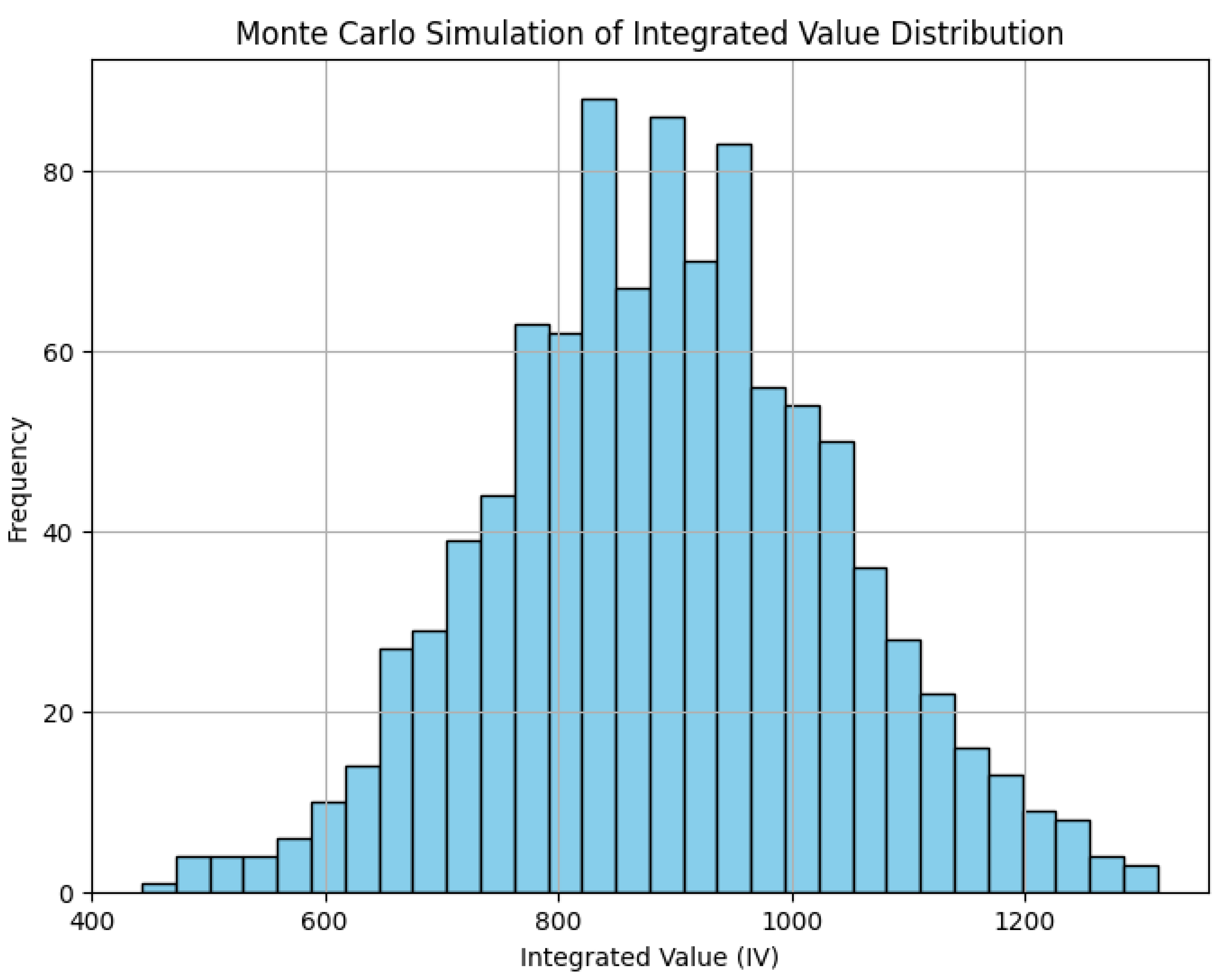
Explanation:

Recognizing that many input parameters in environmental projects are uncertain, this histogram presents a Monte Carlo simulation of the integrated value. In this simulation, we assume that the IV follows a normal distribution (with a mean and standard deviation representing combined uncertainty across dimensions). The histogram shows the range and frequency of potential outcomes, illustrating the risk profile of a project. This type of analysis aids in robust decision-making by highlighting the variability in project valuations under uncertain conditions.

Figure 9. Stacked Bar Chart of Component Contributions to Integrated Value.

Figure 9. Stacked Bar Chart of Component Contributions to Integrated Value.

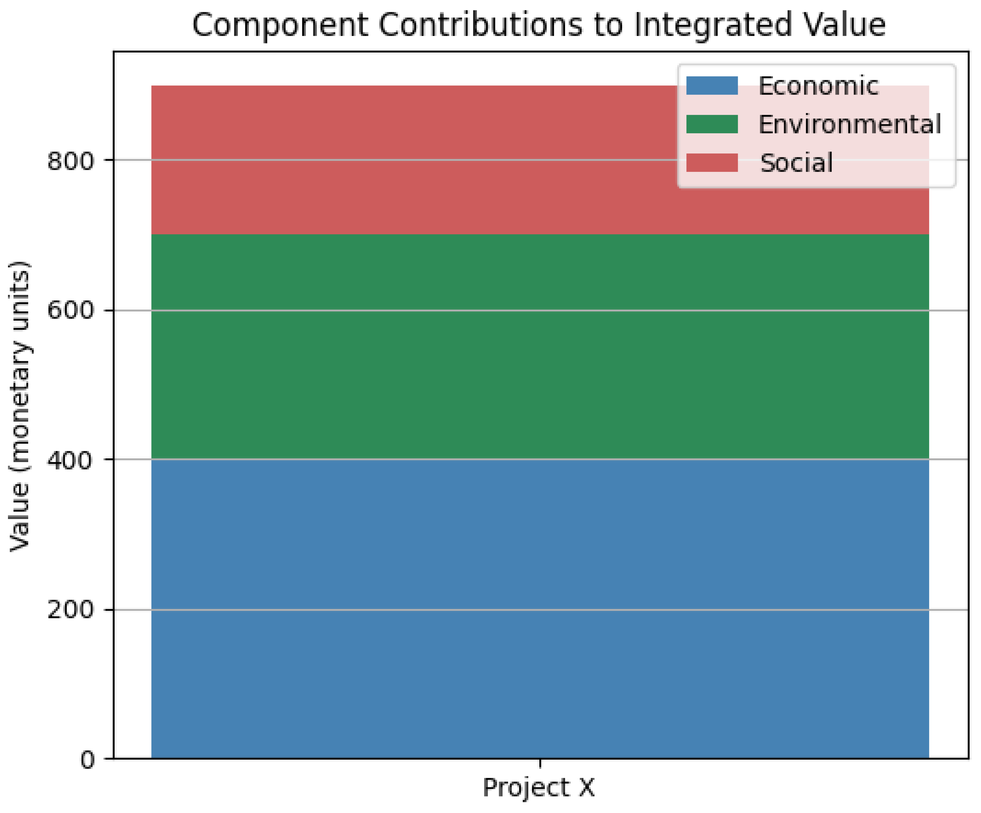
Explanation:

This stacked bar chart compares the relative contributions of the economic, environmental, and social components to the overall integrated value for a selected project scenario. The bar is divided into segments that represent each component’s share. Such a visualization helps decision makers see which dimensions drive the total valuation and can highlight areas where additional benefits (or costs) might be captured. In the example, the economic component forms the base value, with significant contributions added by environmental and social factors.

4. Discussion

The discussion section provides an in-depth analysis of the results, highlighting the strengths and limitations of the model. It also explores the potential applications of the model and acknowledges future research directions.

4.1. Strengths of the Model

The proposed model offers a comprehensive framework for evaluating environmental projects by integrating economic, environmental, and social factors. This holistic approach enables decision-makers to consider the full range of project impacts, rather than focusing solely on financial aspects (Montgomery, 2025). The model’s ability to quantify intangible benefits, such as improved air quality and community well-being, is a significant strength. By assigning monetary values to these benefits, the model provides a more comprehensive evaluation of project outcomes, which is crucial for informed decision-making.

One of the key strengths of the model is its flexibility. It can be adapted to various types of environmental projects, from renewable energy initiatives to conservation efforts. For instance, a renewable energy project aimed at reducing carbon emissions can use the model to assess its economic viability, environmental impact, and social benefits. The model can also be used to evaluate the effectiveness of conservation projects focused on preserving biodiversity and identify areas for improvement.

Another strength of the model is its potential to support policy-making. By providing a comprehensive assessment of project impacts, the model can inform the development of policies that promote sustainable development. For example, the model can be used to evaluate the cost-effectiveness of different policy options for reducing greenhouse gas emissions or promoting biodiversity conservation. This can help policymakers prioritize initiatives that deliver the greatest benefits at the lowest cost.

4.2. Limitations of the Model

Despite its strengths, the model has several limitations. The assignment of monetary values to environmental and social benefits can be subjective and may vary depending on the context. For instance, the value of biodiversity conservation may differ significantly between regions, depending on the local ecosystem and its significance to the community. Additionally, the model relies on the availability of accurate data, which may not always be accessible, particularly in developing countries.

Another limitation is the challenge of capturing long-term impacts. Environmental projects often have benefits that extend over decades, such as the preservation of ecosystems or the reduction of greenhouse gas emissions. Quantifying these long-term benefits in monetary terms can be complex and uncertain. The model may need to be refined to better capture these long-term impacts and incorporate them into the analysis.

4.3. Potential Applications

The model can be applied to a wide range of environmental projects, including renewable energy initiatives, conservation efforts, and sustainable urban development. For example, a renewable energy project aimed at reducing carbon emissions can use the model to assess its economic viability, environmental impact, and social benefits. The model can help identify the most cost-effective technologies and strategies for achieving emission reduction targets.

In the context of conservation efforts, the model can be used to evaluate the effectiveness of different approaches to preserving biodiversity. For instance, it can compare the benefits of establishing protected areas versus implementing community-based conservation programs. The model can also assess the economic and social impacts of these conservation efforts, such as the creation of jobs in ecotourism or the improvement of local infrastructure.

Sustainable urban development projects can also benefit from the model. For example, the model can be used to evaluate the cost-effectiveness of green infrastructure, such as urban parks and green roofs, in improving air quality and reducing urban heat island effects. The model can also assess the social benefits of these projects, such as enhanced community well-being and increased property values.

4.4. Future Research Directions

Future research should focus on refining the model’s methodology for assigning monetary values to environmental and social benefits. This could involve developing more robust valuation techniques that consider the local context and stakeholder preferences. Additionally, the model can be expanded to include more indicators, such as cultural heritage preservation and climate resilience.

Comparative studies can also be conducted to assess the model’s applicability in different regions and contexts. This could involve applying the model to a diverse range of environmental projects in various countries and evaluating its effectiveness in capturing the full range of project impacts. These studies can help identify best practices and areas for improvement in the model’s application.

Another avenue for future research is the integration of the model with other decision-making tools, such as multi-criteria decision analysis (MCDA) and life cycle assessment (LCA). This integration can provide a more comprehensive framework for evaluating environmental projects and support more informed decision-making.

5. Conclusion

The proposed mathematical model for cost-benefit analysis of environmental projects provides a robust framework for evaluating the economic, environmental, and social impacts of such initiatives. By integrating these dimensions, the model offers a comprehensive assessment that supports informed decision-making. The demonstration of the model through Python code and the subsequent analysis of the results highlights its potential applications and limitations.

The model’s ability to quantify intangible benefits, such as improved air quality and community well-being, is a significant advancement in the field of environmental project evaluation. By assigning monetary values to these benefits, the model provides a more comprehensive evaluation of project outcomes, which is crucial for informed decision-making. This is particularly important in the context of environmental projects, where the benefits often extend beyond financial considerations.

The model’s flexibility and potential applications are vast. It can be adapted to various types of environmental projects, from renewable energy initiatives to conservation efforts and sustainable urban development. The model can also support policy-making by informing the development of policies that promote sustainable development. By providing a comprehensive assessment of project impacts, the model can help policymakers prioritize initiatives that deliver the greatest benefits at the lowest cost.

However, the model also has limitations that need to be addressed. The assignment of monetary values to environmental and social benefits can be subjective and may vary depending on the context. The model relies on the availability of accurate data, which may not always be accessible, particularly in developing countries. Additionally, capturing long-term impacts and incorporating them into the analysis remains a challenge.

Future research should focus on refining the model’s methodology and expanding its scope to address these limitations. This could involve developing more robust valuation techniques, expanding the range of indicators, and integrating the model with other decision-making tools. Comparative studies can also be conducted to assess the model’s applicability in different regions and contexts.

In conclusion, the proposed model represents a significant step forward in the evaluation of environmental projects. Its comprehensive approach and potential applications make it a valuable tool for decision-makers and policymakers. However, further research and refinement are needed to fully realize its potential and address the complex challenges of environmental project evaluation.

*The Author declares there are no conflicts of interest.

6. Attachments

import numpy as np

import matplotlib.pyplot as plt

from mpl_toolkits.mplot3d import Axes3D

# Try importing cumtrapz; if unavailable, define a custom function.

try:

from scipy.integrate import cumtrapz

except ImportError:

def cumtrapz(y, x, initial=0):

y = np.asarray(y)

x = np.asarray(x)

dx = np.diff(x)

area = (y[:-1] + y [1:]) / 2 * dx

return np.concatenate(([initial], np.cumsum(area)))

#############################################

# Graph 1: Sensitivity Surface of Integrated Value

#############################################

T = 50 # Time horizon (years)

r_vals = np.linspace(0.01, 0.1, 50) # Discount rates from 1% to 10%

phi_vals = np.linspace(0.5, 2.0, 50) # Environmental conversion factor values

R, Phi = np.meshgrid(r_vals, phi_vals)

# Synthetic function: Economic part discounted + environmental contribution

IV = 1000 * np.exp(-R * T) + Phi * 500

fig = plt.figure()

ax = fig.add_subplot(111, projection=‘3d’)

surf = ax.plot_surface(R, Phi, IV, cmap=‘viridis’)

ax.set_xlabel(‘Discount Rate (r)’)

ax.set_ylabel(‘Environmental Conversion Factor (φ)’)

ax.set_zlabel(‘Integrated Value (IV)’)

ax.set_title(‘Sensitivity Surface of IV as a Function of r and φ’)

fig.colorbar(surf, shrink=0.5, aspect=5)

plt.show()

#############################################

# Graph 2: Temporal Dynamics of Project Values

#############################################

T = 100 # Time horizon in years

t = np.linspace(0, T, 200)

# Simulated time series for each dimension:

EC_t = 1000 * np.exp(-0.03 * t) # Economic value declines over time

ENV_t = 500 * (1 - np.exp(-0.02 * t)) # Environmental value accumulates gradually

SOC_t = 300 + 50 * np.sin(0.1 * t) # Social value oscillates over time

plt.figure()

plt.plot(t, EC_t, label=‘Economic Value (EC(t))’, linewidth=2)

plt.plot(t, ENV_t, label=‘Environmental Value (ENV(t))’, linewidth=2)

plt.plot(t, SOC_t, label=‘Social Value (SOC(t))’, linewidth=2)

plt.xlabel(‘Time (years)’)

plt.ylabel(‘Value (monetary units)’)

plt.title(‘Temporal Dynamics of Project Values’)

plt.legend()

plt.grid(True)

plt.show()

#############################################

# Graph 3: Impact of Risk Aversion on Valuation

#############################################

lambda_vals = np.linspace(0, 1, 100) # Risk aversion coefficient values between 0 and 1

E_IV = 500 # Assumed expected integrated value

variance_IV = 300 # Assumed variance for demonstration

# Risk-adjusted integrated value calculation:

IV_risk = E_IV - lambda_vals * variance_IV

plt.figure()

plt.plot(lambda_vals, IV_risk, linewidth=2)

plt.xlabel(‘Risk Aversion Coefficient (λ)’)

plt.ylabel(‘Risk-Adjusted Integrated Value (IV_risk)’)

plt.title(‘Impact of Risk Aversion on Project Valuation’)

plt.grid(True)

plt.show()

#############################################

# Graph 4: Comparison of Evaluation Methods

#############################################

projects = [‘Project A’, ‘Project B’, ‘Project C’]

economic_only = [300, 450, 200] # Valuations from traditional economic CBA

integrated_framework = [550, 600, 400] # Valuations from the integrated framework

x = np.arange(len(projects))

width = 0.35 # Width of the bars

plt.figure()

plt.bar(x - width/2, economic_only, width, label=‘Economic CBA’)

plt.bar(x + width/2, integrated_framework, width, label=‘Integrated Framework’)

plt.xlabel(‘Projects’)

plt.ylabel(‘Valuation (monetary units)’)

plt.title(‘Project Valuation: Economic CBA vs. Integrated Framework’)

plt.xticks(x, projects)

plt.legend()

plt.grid(True, axis=‘y’)

plt.show()

#############################################

# Graph 5: Sensitivity of IV to Environmental and Social Conversion Factors

#############################################

phi_vals = np.linspace(0.5, 3.0, 50)

psi_vals = np.linspace(0.5, 3.0, 50)

Phi, Psi = np.meshgrid(phi_vals, psi_vals)

# Synthetic function with diminishing returns for both conversion factors:

IV = 200 + (500 * Phi) / (1 + Phi) + (300 * Psi) / (1 + Psi)

fig = plt.figure()

ax = fig.add_subplot(111, projection=‘3d’)

surf = ax.plot_surface(Phi, Psi, IV, cmap=‘plasma’, edgecolor=‘none’)

ax.set_xlabel(‘Environmental Conversion Factor (φ)’)

ax.set_ylabel(‘Social Conversion Factor (ψ)’)

ax.set_zlabel(‘Integrated Value (IV)’)

ax.set_title(‘Sensitivity of IV to φ and ψ’)

fig.colorbar(surf, shrink=0.5, aspect=10)

plt.show()

#############################################

# Graph 6: Integrated Value vs. Time Horizon for Different Discount Rates

#############################################

T = 100

t = np.linspace(0, T, 500)

# Define sample functions for each dimension:

EC = 1000 * np.exp(-0.03 * t) # Economic value declines over time

ENV = 500 * (1 - np.exp(-0.02 * t)) # Environmental value accumulates

SOC = 300 + 50 * np.sin(0.1 * t) # Social value oscillates

phi, psi = 1, 1 # Conversion factors (for simplicity)

total_benefit = EC + phi * ENV + psi * SOC

r_list = [0.02, 0.05, 0.08] # Different discount rates

IV_curves = {}

for r in r_list:

discount_factor = np.exp(-r * t)

discounted_benefit = total_benefit * discount_factor

IV = cumtrapz(discounted_benefit, t, initial=0)

IV_curves[r] = IV

plt.figure(figsize=(8,6))

for r, IV in IV_curves.items():

plt.plot(t, IV, label=f’Discount Rate = {r}’)

plt.xlabel(‘Time Horizon (years)’)

plt.ylabel(‘Cumulative Integrated Value (IV)’)

plt.title(‘IV vs. Time Horizon for Different Discount Rates’)

plt.legend()

plt.grid(True)

plt.show()

#############################################

# Graph 7: Monte Carlo Simulation of Integrated Value Distribution

#############################################

np.random.seed(0) # For reproducibility

n_simulations = 1000

mean_IV = 900 # Assumed mean integrated value

std_IV = 150 # Assumed standard deviation

simulated_IV = np.random.normal(mean_IV, std_IV, n_simulations)

plt.figure(figsize=(8,6))

plt.hist(simulated_IV, bins=30, color=‘skyblue’, edgecolor=‘black’)

plt.xlabel(‘Integrated Value (IV)’)

plt.ylabel(‘Frequency’)

plt.title(‘Monte Carlo Simulation of Integrated Value Distribution’)

plt.grid(True)

plt.show()

#############################################

# Graph 8: Stacked Bar Chart of Component Contributions to Integrated Value

#############################################

EC_value = 400 # Economic contribution

ENV_value = 300 # Environmental contribution

SOC_value = 200 # Social contribution

components = [‘Project X’]

economic = [EC_value]

environmental = [ENV_value]

social = [SOC_value]

x = np.arange(len(components))

plt.figure(figsize=(6,5))

plt.bar(x, economic, width=0.5, label=‘Economic’, color=‘steelblue’)

plt.bar(x, environmental, width=0.5, bottom=economic, label=‘Environmental’, color=‘seagreen’)

plt.bar(x, social, width=0.5, bottom=np.array(economic) + np.array(environmental), label=‘Social’, color=‘indianred’)

plt.xticks(x, components)

plt.ylabel(‘Value (monetary units)’)

plt.title(‘Component Contributions to Integrated Value’)

plt.legend()

plt.grid(axis=‘y’)

plt.show()

References

- Arrow, K. J., Cropper, M. L., Gollier, C., Groom, B., Heal, G. M., Newell, R. G., Nordhaus, W. D., Pindyck, R. S., Pizer, W. A., Portney, P. R., Sterner, T., Tol, R. S. J., & Weitzman, M. L. (2013). Determining benefits and costs for future generations. Science, 341(6144), 349-350. [CrossRef]
- Atkinson, G., & Mourato, S. (2008). Environmental cost-benefit analysis. Annual Review of Environment and Resources, 33, 317-344.
- Barbier, E. B. (2011). Capitalizing on Nature: Ecosystems as Natural Assets. Cambridge University Press.
- Bateman, I. J., Mace, G. M., Fezzi, C., Atkinson, G., & Turner, K. (2011). Economic analysis for ecosystem service assessments. Environmental and Resource Economics, 48(2), 177-218. [CrossRef]
- Belton, V., & Stewart, T. J. (2002). Multiple Criteria Decision Analysis: An Integrated Approach. Kluwer Academic Publishers.
- Boardman, A., Greenberg, D., Vining, A., & Weimer, D. (2017). Cost-Benefit Analysis: Concepts and Practice. Cambridge University Press.
- Carson, R. T. (2012). Contingent valuation: A practical alternative when prices aren’t available. Journal of Economic Perspectives, 26(4), 27-42. [CrossRef]
- Costanza, R., de Groot, R., Sutton, P., van der Ploeg, S., Anderson, S. J., Kubiszewski, I., Farber, S., & Turner, R. K. (2014). Changes in the global value of ecosystem services. Global Environmental Change, 26, 152-158. [CrossRef]
- Daly, H. E. (2007). Ecological Economics and Sustainable Development: Selected Essays of Herman Daly. Edward Elgar Publishing.
- Dasgupta, P. (2008). Discounting climate change. Journal of Risk and Uncertainty, 37(2-3), 141-169.
- de Groot, R. S., Alkemade, R., Braat, L., Hein, L., & Willemen, L. (2010). Challenges in integrating the concept of ecosystem services and values in landscape planning, management and decision making. Ecological Complexity, 7(3), 260-272. [CrossRef]
- Farrow, S. (2004). Using risk assessment, benefit-cost analysis, and real options to implement a precautionary principle. Risk Analysis, 24(3), 727-735. [CrossRef]
- Forsyth, T. (2003). Critical Political Ecology: The Politics of Environmental Science. Routledge.
- Gollier, C. (2002). Discounting an uncertain future. Journal of Public Economics, 85(2), 149-166.
- Gollier, C., & Weitzman, M. L. (2010). How should the distant future be discounted when discount rates are uncertain? Economics Letters, 107(3), 350-353.
- Goulder, L. H., & Williams, R. C. (2012). The choice of discount rate for climate change policy evaluation. Climate Change Economics, 3(04), 1250024. [CrossRef]
- Gowdy, J., Howarth, R. B., & Tisdell, C. (2010). Discounting, ethics, and options for maintaining biodiversity and ecosystem integrity. In P. Kumar (Ed.), The Economics of Ecosystems and Biodiversity: Ecological and Economic Foundations (pp. 257-283). Earthscan.
- Hanley, N., & Barbier, E. B. (2009). Pricing Nature: Cost-Benefit Analysis and Environmental Policy. Edward Elgar Publishing.
- Heal, G., & Millner, A. (2014). Reflections: Uncertainty and decision making in climate change economics. Review of Environmental Economics and Policy, 8(1), 120-137.
- Hicks, J. R. (1939). The foundations of welfare economics. The Economic Journal, 49(196), 696-712.
- Howarth, R. B., & Norgaard, R. B. (2013). Intergenerational transfers and the social discount rate. Environmental and Resource Economics, 3(4), 337-358. [CrossRef]
- IPCC. (2022). Climate Change 2022: Impacts, Adaptation and Vulnerability. Cambridge University Press.
- Just, R. E., Hueth, D. L., & Schmitz, A. (2004). The Welfare Economics of Public Policy: A Practical Approach to Project and Policy Evaluation. Edward Elgar Publishing.
- Kaldor, N. (1939). Welfare propositions of economics and interpersonal comparisons of utility. The Economic Journal, 49(195), 549-552. [CrossRef]
- Montgomery R. M. (2025). Investigating Coexistence and Extinction in a Four-Species Trophic System Using Random Matrix Theory. Journal of Medicine and Healthcare. SRC/JMHC-375. [CrossRef]
- Mongomery, R. M. (2024). Topological Dynamics in Ecological Biomes and Toroidal Structures: Mathematical Models.
- Montgomery, R. M. (2024)a. Techniques for Outlier Detection: A Comprehensive View. Journal of Biomedical and Engineering Research.2 (2), 1-10.
- of Stability, Bifurcation, and Structural Failure. J Gene Engg Bio Res, 6(2), 01-09.
- Nordhaus, W. D. (2007). A review of the Stern Review on the economics of climate change. Journal of Economic Literature, 45(3), 686-702. [CrossRef]
- O’Neill, J., Holland, A., & Light, A. (2008). Environmental Values. Routledge.
- Pearce, D., Atkinson, G., & Mourato, S. (2006). Cost-Benefit Analysis and the Environment: Recent Developments. OECD Publishing.
- Polasky, S., Carpenter, S. R., Folke, C., & Keeler, B. (2011). Decision-making under great uncertainty: Environmental management in an era of global change. Trends in Ecology & Evolution, 26(8), 398-404.
- Spash, C. L. (2008). How much is that ecosystem in the window? The one with the bio-diverse trail. Environmental Values, 17(2), 259-284. [CrossRef]
- Stern, N. (2007). The Economics of Climate Change: The Stern Review. Cambridge University Press.
- Sunstein, C. R. (2018). The Cost-Benefit Revolution. MIT Press.
- Turner, R. K., Pearce, D., & Bateman, I. (1994). Environmental Economics: An Elementary Introduction. Harvester Wheatsheaf.
- Vatn, A. (2009). An institutional analysis of methods for environmental appraisal. Ecological Economics, 68(8-9), 2207-2215. [CrossRef]
- Weitzman, M. L. (2001). Gamma discounting. American Economic Review, 91(1), 260-271.
- Weyant, J. (2017). Some contributions of integrated assessment models of global climate change. Review of Environmental Economics and Policy, 11(1), 115-137. [CrossRef]
- Wilson, M. A., & Howarth, R. B. (2002). Discourse-based valuation of ecosystem services: Establishing fair outcomes through group deliberation. Ecological Economics, 41(3), 431-443. [CrossRef]
Disclaimer/Publisher’s Note: The statements, opinions and data contained in all publications are solely those of the individual author(s) and contributor(s) and not of MDPI and/or the editor(s). MDPI and/or the editor(s) disclaim responsibility for any injury to people or property resulting from any ideas, methods, instructions or products referred to in the content. |
© 2025 by the authors. Licensee MDPI, Basel, Switzerland. This article is an open access article distributed under the terms and conditions of the Creative Commons Attribution (CC BY) license (http://creativecommons.org/licenses/by/4.0/).
Copyright: This open access article is published under a Creative Commons CC BY 4.0 license, which permit the free download, distribution, and reuse, provided that the author and preprint are cited in any reuse.