Submitted:
06 May 2025
Posted:
07 May 2025
You are already at the latest version
Abstract
In this paper we study an ODE model for the interaction between nature and society where the system dynamics is driven largely by the social wealth. The relevant variables are renewable resources, non-renewable ones, and wealth, while population depends on wealth and does not act on the other variables. We first obtain that the relevant trajectories are positive and cannot grow arbitrarily large. Then we compute all the equilibria and study their stability. We also give numerical simulations of some trajectory.
Keywords:
human and nature dynamics
; ODE systems for society dynamics
; ecological–economic modeling
1. Introduction
This paper continues a research that we have carried out in our three previous works [1,2,3]. In all these papers we introduced low-dimension ODE systems intended to model the interactions between society and natural resources. The models in the quoted papers deal with four variables: x is the population, y the level of renewable resources, z the level of non-renewable resources, w the wealth produced using and depleting the resources. In this paper we introduced a model dealing only with . This derives from the effort to study a model able to capture some characteristics of modern wealthy societies. In this kind of societies population is less or more stationary (or slowly decreasing) and the dynamics of interaction between society and resources is led by other variables. In [3] we introduced an ODE system in which the dynamics is led by non-renewable resources, while in the present paper we study a model in which the evolution is driven by the wealth w. The system is the following
Here, are as we said above, while are positive coefficients. The equations for is the usual logistic equation, with a depletion term . This means that the rate of depletion is given by the level of wealth in the society. In the same way, the equation for has a depletion term with rate of depletion . There is also, in the equation for z, a replenishment term, which says that human ingenuity is able to find new sources of non-renewable resources. The replenishment term depends only on w and is given through the function , which is a saturation function of the type used in population dynamics. This term means that there is a replenishment of this kind of resources, but its rate is bounded. Finally, the equation for states that wealth increases thanks to the use of resources (renewable and non-renewable) and decreases because of consumption () and because of the investment needed to replenish non-renewable resources (). In the present model, differently from our previous papers, the rate of consumption depends on w, to be coherent with the idea to study a model in which the dynamics is driven by w.
We now briefly describes the main result of this paper (see also the conclusions, section 8). As we are interested on the trajectories with positive or non negative component, we first have proved that relevant trajectories remain positive. We then prove that none of the variables can diverge to , which means, in particular, that there can’t be indefinite growth in wealth. We then compute the equilibrium points of the system, and we study their stability. In some cases, due to the difficulty of this study, we get stability or instability results only when the depletion coefficients . We obtain that there are stable equilibria with positive values for all the variables, at least for some range of the parameters.
The search for mathematical models to investigate global social evolution and highlight the risks of collapse has nowadays a long tradition, starting at least with the celebrated work of the MIT group on the "Limits to growth": see the books [4,5,6], the update [7] and also [8]. The models introduced by the MIT group are high dimensional, and are studied through numerical computations. More recently some low dimensional model has been proposed for the same purposes. Our work started, in [1], from the HANDY model, which has been introduced in [9,10], and has then been studied by various authors (see [11,12,13,14,15,16,17,18]). After [1] we have changed in various way our models, so the problems studied in [2,3] and in the present paper can not be anymore considered examples of HANDY models. See also [19] for another model of interactions between society and nature. The main contribution of our research (including the present paper and the quoted ones) to this debate lies in the fact that, even assuming a moderate optimism on the replenishment of non-renewable resources, the aim of an indefinite growth in wealth seems impossible to attain, and also disruptive for the society. During our research, we have obtained this kind of results with different hypotheses on the main drivers of societal evolution, so they seem to have some kind of robustness (using the word in a non rigorous sense).
The paper is organized as follows: after the introduction, in section 2 we prove that the relevant trajectories are defined and non negative for all , and that they cannot go to . In section 3 we compute all the equilibria of system (1). In the following sections 4, 5, 6, we analyze the stability of the equilibria. In section 7 we show some numerical simulations and in section 8 we present a summary of the main results obtained.
2. General Results
We are interested in non-negative solutions of (1) hence, as in our previous papers, we will work in the positive cone defined as
or in its closure
Let be the vector field of the system (1). Note that . Thus, we have a standard result of existence and uniqueness:
Proposition 1.
For any and , there exists a unique solution to the Cauchy problem
defined on a maximal interval with .
If , we assume , that is, we assume that the social-nature evolution we study starts with a positive amount of renewable and non-renewable resources, while the starting social wealth is positive or zero. However, the next proposition shows that the case can be dealt with in a very easy way.
Proposition 2.
Let with . Let be the solution of the logistic equation
Then the function is the unique solution of the Cauchy problem:
Proof.
The proof follows from a straightforward computation. □
Proposition 2 shows that, when the initial value is zero, the solution is known, and no further analysis is necessary. For this reason, from now on, we assume , that is, we will study system (1) with initial condition . We will also assume .
Proposition 3.
Let be a solution of (2) with and . Then for all .
Proof.
From Proposition 2, we know that for all . On the other hand, the two equations for and have the zero constant as a solution for all , hence this constant cannot be crossed by another solution, ensuring that and remain positive for all . □
Proposition 4.
Let and be the solution of (2) with . Then is bounded on .
Proof.
We distinguish two cases
for all : in this case for all t, hence for all t, hence is bounded.
for some . Let us define
If we have for all , so is obviously bounded in . If we assume then , by continuity, it is easy to obtain , for all , , so that . On the other hand, using the equation for , we get
This is a contradiction, so this case is ruled out, hence and y is bounded.
□
Proposition 5.
Under the same assumptions, we have .
Proof.
We argue by contradiction. Assume . Consider the variable , which satisfies for all , hence for all . Consequently, for all , so it is bounded in . Similarly, for , recalling that is bounded, we have , hence on . Therefore, on , implying that is bounded on . Thus, is bounded on , which contradicts the standard ODE theory. Therefore, . □
Proposition 6.
It cannot happen that .
Proof.
Assume by contradiction that . Then we have , and given that
we obtain that there exists such that for all . Therefore, is decreasing on and has a limit . If , then , which contradicts well-known theorems. Hence . Now, consider . Since is bounded, , and , there exists such that for all . This implies for all , which contradicts the assumption . The thesis is thus proved. □
Proposition 7.
It cannot happen that .
Proof.
We will prove that implies , and by Proposition 6 this is a contradiction, hence the thesis. So, assume as . Fix and such that for all .
We consider the following cases:
- Assume for all . This implies on , hence there exists a limit . If , recalling that , from we would obtain , a contradiction with well-known theorems. Hence, it must be , that is, , but this contradicts Proposition 6. Thus, we can rule out this case, meaning that it is not possible that
-
Therefore, there exists such thatNow, let us pick . Ifwe obtain because hence . On the other hand, assumeDefineBy continuity, we get , for all , and . Hence, on , so . We have thus proved that for all , it holds that . Therefore, for any , there exists such that for all , which meansThis is ruled out by Proposition 6, so we have obtained a contradiction, and the thesis is proved.
□
3. Equilibrium Points
Equilibrium points are the solutions of the following system:
Let us consider the different possible cases:
- 1)
- , no conditions on z. We obtain a family of equilibria with .
- 2)
- , , . In this case, we obtain the equilibrium , which is not in , so it is not of interest.
- 3)
-
, , . In this case, from (), we obtain the equation for w:which has the solutionsand we assume of course For z we obtain, from equation (),Hence, we have two equilibria:
- 4)
- , . We obtain and no conditions on z, so we have a family of equilibria:
- 5)
-
, , . In this case, we obtain the linear system:whose solutions areThus, we obtain an equilibrium:
- 6)
- , , . As before, we obtain the two values , given in (6) for the variable w, while the values for y and z are now given bygiving rise to two steady states:
4. Stability of Equilibria: Cases 1 and 3
The Jacobian matrix of the vector field at a point is given by:
Let us now analyze the stability of the equilibria previously identified. We will not consider case 2) because, as we have seen above, the equilibrium is not in .
4.1. Case 1
In case 1), we have , so the first row of the Jacobian matrix is the vector . This means that is an eigenvalue, hence all these equilibria are unstable.
4.2. Case 3
In case 3), we also have , so the first row of the Jacobian matrix is the vector . This means that is an eigenvalue. We will obtain asymptotic results as for . In this section we will assume, for simplicity, linear relations between the coefficients . Specifically, we assume , , and with , and we will study the asymptotic behavior of equilibria as . Now we want to obtain the asymptotic developments of w. Recall that
Let us now find what happens as . First, we have
hence
For the equilibrium we obtain the eigenvalue , indicating that this is an unstable equilibrium, as . For the equilibrium the eigenvalue becomes
Therefore, if , the equilibrium is also unstable for . Let us now analyze the case . We have
so the entry of the Jacobian matrix (13), computed at the points (12), becomes
Hence, the Jacobian matrix in this case becomes
We have
We obtain the following developments:
As a consequence, we have
Given these asymptotic expansions, we obtain
This matrix has an eigenvalue and we are assuming , hence as . The other eigenvalues are obtained from the submatrix
We have Trace()= and Det()=, so the eigenvalues of have negative real part as . Hence all the eigenvalues of have negative real part, and is an asymptotically stable equilibrium. The following proposition summarizes the results of this section
Proposition 8.
All the equilibria of Case 1 are unstable (for any value of the parameters). As to Case 3, the equilibrium is unstable as , while equilibrium is unstable if and is asymptotically stable if (and ).
5. Stability of Equilibria: Case 4
In case 4 the equilibria are given by with , and the Jacobian matrix is
The eigenvalues are , , and . If , then and the equilibria are unstable. Let us study the case , that is, . In this case the study of the Jacobian matrix is not useful, because two eigenvalues are negative and one is zero. We will however obtain a stability result with an ad hoc argument. We will deal only with trajectories starting in , because in our model these are the relevant trajectories. Let us start by introducing the rectangular neighborhoods of P as follows, for :
After this we introduce the constants as follows: since , it is possible to choose two positive numbers such that for all , the following holds:
Also we pick such that , that is, .
We then state the result we are going to prove:
Proposition 9.
There is such that for all there is such that, if we pick and we call the trajectory starting from Q at , then for all . Also, it holds:
- are decreasing function, and for all .
- .
- There exists a positive constant , independent of ϵ and , such that the following holds:
Notice that Proposition 9 states that P is Lyapunov-stable and give some information on the asymptotic behavior of the variables as , but does not imply asymptotic stability. Indeed, if , does not converge to Z.
The proof of Proposition 9 will be done in several steps.
Step 1: For any , if , then for all .
Proof.
By the arguments of Proposition 4 it is to get that , and if , then obviously . □
Step 2: Assume and , , . Then it holds and for all .
Proof.
As it is easy to get
Hence we get
As a consequence, there exists such that for all , it holds and .
Now we define
We know that . We want to prove that , which gives the thesis. Let us consider all other possible cases and show that they lead to a contradiction.
- i)
- If then ; we have for all , hence . Therefore,implying for . Since , we obtain a contradiction with the definition of .
- ii)
- If we have for all , hence . Therefore,hence for all . Since , this is a contradiction with the definition of .
- iii)
-
If , by continuity, we easily obtain and on , with . Therefore, as above, for all , and on , hence , which is a contradiction.Thus, the only possibility left is , which proves the thesis.
□
Step 3: Hypotheses as in Step 2. Then, it is for all .
Proof.
By the previous steps we know that and for all . Using the equation for we obtain, as in Step 2:
and a simple integration gives the result.
□
Step 4: Hypotheses as in Step 2. Then there exist a positive constants , independent of and , such that the following holds:
Proof.
The inequality is obvious from Step 2. Now, using Step 3 and the equation for in the model (1), we have
hence , so that
so that with .
□
Step 5: There are and sucht that, if , , , and , then for all .
Proof.
Notice that the thesis is obvious if , because is decreasing and positive. Hence we assume . Let us take . We have for all , by the hypotheses and the previous Steps. Now, assume and define
Let us pick and consider the inequality
By the standard asymptotic development of this is equivalent to
and by simple computations this is equivalent to
By our choice of , we get that there is such that for all the inequality (18) holds, and of course we can choose . Now from (18) we deduce, as and ,
so that
and we get the result thanks to Step 4.
□
For the next Step 6, we introduce , and we notice that for all and all it is .
Step 6: Pick and . Assume , , . Then for all .
Proof.
By the equation for and the previous Steps we get
where . Let us consider the function which is the solution of the following logistic Cauchy problem:
By standard comparison principles we obtain for all . Now, the well-known properties of logistic equation give that, if then for all , hence for all . On the other hand, if , we know that for all t, so also , by our choice of . The proof of Step 6 is now complete.
□
Step 7: Assume the hypotheses of Step 6. Then it is .
Proof.
We will study and , and we will prove that they are equal. Let us start by proving that . We use the arguments of Proposition 4, and we distinguish two cases, as we did there:
for all : in this case we know that for all t, so there exists and it holds . If then, recalling Step 3,
which is a contradiction with standard result. Hence , which trivially implies .
for some : in this case we have proved, in Proposition 4, that for all , which of course implies .
So we get, in any case, . Let us now prove that . Fix any , and pick such that for all it holds . From the equation for we get
where and the inequality holds for all . Now we pick the value and consider the function which is the solution of the following logistic Cauchy problem
As , standard results give that is increasing for and . On the other hand, an easy application of comparison principles gives that for all , hence . As this hold for all , we get .
We can now conclude the argument: we have obtained , and this obviously implies
The thesis is proved.
□
Step 8: We now end the proof of Proposition 9: it is enough to choose and and, for any , to define . The previous Steps give all the result stated in Proposition 9.
Let us now collect the result of this section.
Proposition 10.
Let with . If , then the equilibrium point P is unstable. If , then P is Lyapunov-stable and the asymptotic result of Proposition 9 hold.
Remark 1.
We notice that the results of this section are not asymptotic results, but hold for any value of the parameters, provided the hypotheses are satisfied.
6. Stability of Equilibria: Cases 5 and 6
We now deal with cases 5 and 6. As in section 3 we will study the stability and instability properties of equilibria when and we will assume, for simplicity, linear relations between the coefficients . So, as above, we set , , and with , and we will study the asymptotic behavior of equilibria as . This approach rules out case 5) because, as , from (9) we get , so the steady state is not in . We can repeat the same computations of Case 3, obtaining that the Jacobian matrix (13), computed at the points (12), is as follows:
Now we want to obtain the asymptotic developments of y, z, and w. For the values () the same computations of Case 3 hold, while for we use 11. Hence we have, for ,
Looking at the Jacobian matrix (21), we obtain in this case
Considering
we have
Hence, the Jacobian matrix is given by
Its determinant is given by Det. Denoting by = Det its characteristic polynomial, we obtain DetDet as . As lower order terms, we obtain that has a real positive root, which is a real positive eigenvalue of . We then deduce that the equilibrium is unstable as .
Let us now see what happens for . We have:
We note that if , which is true only if the previously encountered condition is satisfied. From now on, we will consider this condition valid so that remains in .
Looking at the Jacobian matrix (21), we obtain in this case:
Now we notice that
so that we have:
Hence, the Jacobian matrix is given by:
Denoting by its characteristic polynomial, we obtain:
We apply now the Routh-Hurwitz criterion (see [20]). As we are assuming , we have .So we need only to check if . We have
as , so we have asymptotic stability.
The following proposition summarizes the results of this section.
Proposition 11.
When we have the following results:
- i)
- The equilibrium of Case 5 is not in .
- ii)
- The equilibrium of Case 6 is always unstable.
- iii)
- The equilibrium of Case 6 is asymptotically stable if and it is outside if .
Remark 2.
If , that is , we obtain the condition that we found in our previous works.
7. Simulations
We now present the results obtained from simulations conducted using Matlab’s ode45 solver, which utilizes an explicit adaptive Runge-Kutta method. The goal of these simulations was to verify our theoretical analyses. We display our findings in two formats: Cartesian graphs in scenarios where instability is more pronounced and phase diagrams in cases of stability where these representations provide clearer insights.
In the Cartesian graphs shown, the evolution of the variables is depicted by introducing small perturbations to the initial conditions around the equilibrium point. Different colors represent the variables: green for renewable resources, black for non-renewable resources and blue for accumulated wealth. Dashed lines indicate the coordinates of the equilibrium point under consideration, with the color corresponding to each specific component (e.g., blue for wealth). The x-axis is labeled with a generic time unit that does not correspond to specific intervals such as days, months, or years, but instead represents a general time scale that may not cover extended periods. The simulation is terminated once the system’s behavior becomes evident.
The phase diagrams illustrate the behavior of renewable or non-renewable resources and wealth in proximity to the steady states discussed in our study. These diagrams focus on two main variables, plotting three distinct trajectories (depicted in magenta, dark green and red) generated by applying three different perturbations around the critical point within a two-dimensional space. The graphs highlight stable points, where the dynamics naturally lead the system towards equilibrium. Initial points are marked with small circles, while steady states are indicated by small stars.
7.1. Case 3
We wanted to test a stable situation with . We considered the following parameter values: , that is , resulting in the stable point with . In Figure 1 we have represented the phase diagrams obtained by considering non-renewable resources versus wealth on the left, and renewable resources versus wealth on the right. The Jacobian matrix calculated at has eigenvalues .
We also tested, without displaying the graph, some cases of instability, noting that the trajectories, in this situation, stabilize at the point denoted as in Case 6. Specifically, by varying the parameter in Case 3, we obtain with a critical point and convergence to , which corresponds to the point with the same parameters as in Case 6.
7.2. Case 4
In the simulations for the scenario described in Case 4, we considered the parameters , starting from the critical point with ; since we want to study , we have set .
In Figure 2, we show the simulations related to ; on the left, we started with a positive perturbation on the coordinate , while applying a negative perturbation to and . In the Figure 2 on the right, all perturbations are positive. As predicted by the theory, the trajectories of the variables and decrease, while . We note that for both graphs, we have convergence , while the trajectory of behaves differently. Furthermore, the convergence of the variable varies depending on the magnitude of the input perturbation and its relationship with Z. The Jacobian matrix calculated at the point has the following eigenvalues: .
7.3. Case 6
Figure 3 shows the simulations related to the point obtained with , i.e. and , which is a stable point. The eigenvalues of the Jacobian matrix calculated here are . We note that this is a stable situation where all variables are strictly positive.
8. Conclusions
We now summarize the main results of this paper. First, we have obtained that for the trajectories in it can’t happen or or , as . Of course, this does not mean that this variables remain bounded, but that there is a positive constant C such that if, for example, at a time , then w must go below C at a time . So an excessive growth in wealth generates oscillations, and these are phenomena that generally have negative social consequences. Another relevant result is the following: although we have obtained that many equilibria of the system are unstable (or are outside ), there are still, at least for some range of the parameters, stable equilibria with positive values for all the variables (see Proposition 11 and Figure 3). We note that all numerical simulations confirm the theoretical results obtained. From these results a general indication seems to emerge: assuming the hypotheses of the model, an indefinite growth in wealth is not a reasonable aim, while it seems possible to drive the society towards a steady state with positive values of all the variables, at least for small rates of exploitation of resources. Hence, the results of our works (the present one and the previous papers [1,2,3]) are in line with the ideas of those who support the need to abandon the idea of infinite growth and instead to search a path towards stationary economic situations, possibly through a period of degrowth.
These results are similar to those that we have obtained in our previous papers, using similar but different models. This seems to us a relevant achievement in itself, because it means that these results are very stable with respect to changes in the model. Despite the fact that, in any case, all the models that we have studied, in the present and the previous papers, are of course too simple to allow precise predictions on social evolution, this stability of the qualitative ideas that they suggest may be an interesting contribution to the debate on the future of our societies.
Author Contributions
Conceptualization, M. B.; Methodology, M. B. and I. C.; Software, I. C.; Formal analysis, M. B. All authors have read and agreed to the published version of the manuscript.
Funding
This research received no external funding.
Data Availability Statement
Data are contained within the article.
Conflicts of Interest
The authors declare no conflict of interest.
References
- Badiale, M.; Cravero, I. A HANDY-type model with non-renewable resources. Nonlinear Analysis: Real World Applications 2024, 77, 104071. https://www.sciencedirect.com/science/article/pii/S1468121824000117. [CrossRef]
- Badiale, M.; Cravero, I. A Nonlinear ODE Model for a Consumeristic Society. Mathematics 2024, 12, 1253. [CrossRef]
- Badiale, M.; Cravero, I. A Nonlinear ODE Model for a Society Strongly Dependent on Non-Renewable Resources. AppliedMath 2025, 5. [CrossRef]
- Meadows, D.H.; Meadows, D.L.; Randers, J. Beyond the limits: Confronting global collapse, envisioning a sustainable future; Chelsea Green Publishing Co.: White River Junction, VT, 1992.
- Meadows, D.H.; Meadows, D.L.; Randers, J. The limits to growth: The 30-year update; Chelsea Green Publishing Co.: White River Junction, VT, 2004.
- Meadows, D.H.; Meadows, D.L.; Randers, J.; Behrens, W.W. The limits to growth: A report for the Club of Rome’s project on the predicament of mankind; Universe Books: New York, 1972.
- Herrington, G. Update to limits to growth: Comparing the World3 model with empirical data. Journal of Industrial Ecology 2022, 26, 312–324. [CrossRef]
- Murphy, T.W. Limits to economic growth. Nature Physics 2022, 18, 844–847. [CrossRef]
- Motesharrei, S.; Rivas, J.; Kalnay, E. Human and nature dynamics (HANDY): Modeling inequality and use of resource in the collapse or sustainability of societies. Ecological Economics 2014, 101, 90–102. [CrossRef]
- Motesharrei, S.; Rivas, J.; Kalnay, E.; Asrar, G.; Busalacchi, A.; Cahalan, R.; Cane, M.; Colwell, R.; Feng, K.; et al., R.F. Modeling sustainability: Population, inequality, consumption, and bidirectional coupling of the Earth and Human Systems. National Science Review 2016, 3, 470–494. [CrossRef] [PubMed]
- Akhavan, N.; Yorke, A. Population collapse in Elite-dominated societies: a differential model without differential equations. SIAM J. Appl. Dyn. Syst. 2020, 19, 1736–1757. [CrossRef]
- Al-Khawaja, T. Mathematical Models, Analysis and Simulations of the HANDY Model with Middle Class. PhD thesis, Oakland University, Rochester, MI, USA, 2021. https://our.oakland.edu/handle/10323/11946 (accessed on 20 March 2024).
- Castro, R.; Fritzson, P.; Cellier, F.; Motesharrei, S.; Rivas, J. Human-Nature Interaction in World Modeling with Modelica. In Proceedings of the Proceedings of the 10th International Modelica Conference, Lund, Sweden, 2014; pp. 477–488. [CrossRef]
- Grammaticos, B.; Willox, R.; Satsuma, J. Revisiting the Human and Nature Dynamics Model. Regular and Chaotic Dynamics 2020, 25, 178–198. https://arxiv.org/pdf/1911.05533.
- Sendera, M. Data adaptation in handy economy-ideology model. https://arxiv.org/abs/1904.04309.
- Shillor, M.; Kadhim, T. Analysis and simulation of the HANDY model with social mobility, renewables and nonrenewables. Electronic Journal of Differential Equations 2023, 2023, 1–22. https://ejde-ojs-txstate.tdl.org/ejde/article/download/360/332.
- Tonnelier, A. Sustainability or societal collapse, dynamics and bifurcations of the handy model. SIAM Journal on Applied Dynamical Systems 2023, 22, 1877–1905. [CrossRef]
- Yang, Z.; Abdollahian, M.; Neal, P. Social Spatial Heterogeneity and System Entrainment in Modeling Human and Nature Dynamics. In Proceedings of the Theory, Methodology, Tools and Applications for Modeling and Simulation of Complex Systems; Zhang, L.; Song, X.; Wu, Y., Eds., Singapore, 2016; pp. 311–318.
- Nitzbon, J.; Heitzig, J.; Parlitz, U. Sustainability, collapse and oscillations in a simple World-Hearth model. Environmental Research Letters 2017, 12, 074020. [CrossRef]
- Gantmacher, F.R. The theory of matrices volume 2; AMS Chelsea Publishing, 2000.
Figure 1.
Case 3. Phase diagram related to the analysis of the stable point . On the left: non-renewable resources versus wealth. On the right: renewable resources versus wealth.
Figure 1.
Case 3. Phase diagram related to the analysis of the stable point . On the left: non-renewable resources versus wealth. On the right: renewable resources versus wealth.
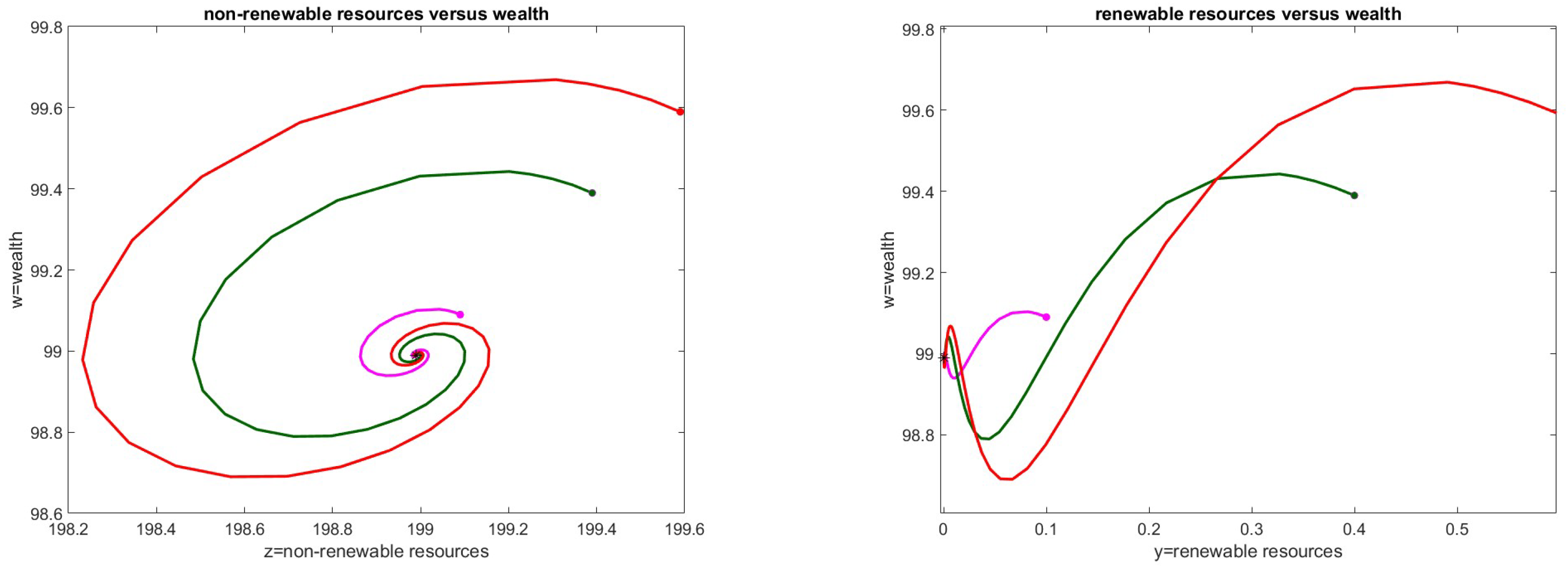
Figure 2.
Case 4. The variable z stabilizes at a value different from the critical one. On the left: negative perturbations on and . On the right: all initial perturbations are positive.
Figure 2.
Case 4. The variable z stabilizes at a value different from the critical one. On the left: negative perturbations on and . On the right: all initial perturbations are positive.
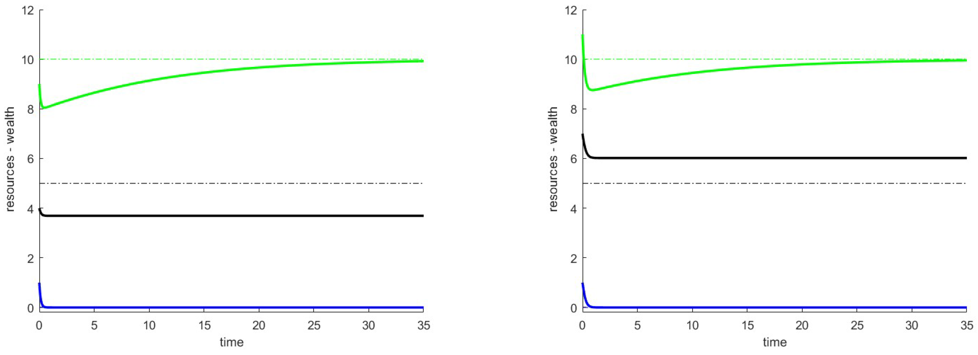
Figure 3.
Case 6. Phase diagram related to the analysis of the stable point . On the left: non-renewable resources versus wealth. On the right: renewable resources versus wealth.
Figure 3.
Case 6. Phase diagram related to the analysis of the stable point . On the left: non-renewable resources versus wealth. On the right: renewable resources versus wealth.

Disclaimer/Publisher’s Note: The statements, opinions and data contained in all publications are solely those of the individual author(s) and contributor(s) and not of MDPI and/or the editor(s). MDPI and/or the editor(s) disclaim responsibility for any injury to people or property resulting from any ideas, methods, instructions or products referred to in the content. |
© 2025 by the authors. Licensee MDPI, Basel, Switzerland. This article is an open access article distributed under the terms and conditions of the Creative Commons Attribution (CC BY) license (http://creativecommons.org/licenses/by/4.0/).
Copyright: This open access article is published under a Creative Commons CC BY 4.0 license, which permit the free download, distribution, and reuse, provided that the author and preprint are cited in any reuse.


