Submitted:
10 January 2025
Posted:
13 January 2025
You are already at the latest version
Abstract
In this work we study an ODE system intended to model the interaction between nature and society in the case of a society heavily dependent on non-renewable resources. In the model this dependence translates into the fact that the rates of consumption of resources and wealth depend on non-renewable resources. We first obtain that the relevant trajectories of the system are bounded, then we compute all the equilibria of the system and study their stability.
Keywords:
human and nature dynamics
; ODE systems for society dynamics
; ecological-economic modeling
1. Introduction
In this paper we pursue a line of research that we started in our two previous papers [1,2]. Our aim is to elaborate some simple nonlinear ODE models to describe the interaction between human society and nature, paying attention in particular to the use of renewable and non-renewable resources. In [1] we started from the HANDY model, which has been introduced in [3] (see also [4]) and then studied by several authors (see [5,6,7,8,9,10]). Our work was linked in particular with [10], who simplified and clarified the original HANDY model, and [9], who introduced non-renewable resources. In the paper [2] we introduced a different model, which can not anymore be considered a HANDY model. Our present paper is linked to [2], so we will discuss analogies and differences between the present paper and [2].
The model that we will study in the present paper is the following:
Here x is the variable for the population, y the variable for renewable resources, z the one for non-renewable resources, w the one for wealth. c, d, , , , k, , are positive parameters. The equation for describes the fact that the population is decreasing when the value , that is wealth per capita via a parameter, is very small or very big. This seems to fit the reality of contemporary rich societies better then the original HANDY model, in which a rich population grows with a positive rate. In the other three equations we have depletion terms whose rate of depletion is lead by z, the non-renewable resources, not by population x or wealth w. This is the main difference with respect to previous models, like HANDY-type models or our previous one expounded in [2]. The dynamics in this model are largely driven by non-renewable resources, and we think that this could be a good way to capture some relevant features of contemporary industrialized societies, which indeed strongly depend on non-renewable resources like oil.
Let us now describe the equation for . The equations for is a standard logistic one, with a depletion term . The equation for has a depletion term with rate of depletion , giving rise to the term . There is also a replenishment term, which is a novelty introduced in our papers, to describe the fact that human ingenuity is able to find new sources of non-renewable resources, or maybe new non-renewable resources (oil instead of coal, for example). The replenishment term has the form , where the replenishment rate is driven by w and z, and the function is a saturation function of standard use in population dynamics. This term modelize a moderate optimism on non-renewable resources: there is a replenishment of this kind of resources, but its rate is bounded. Finally, the equation for states that wealth increases thanks to the use of resources (renewable and non-renewable) and decreases because of consumption. In the present model, differently from our previous papers, the rate of consumption depends on z, again to underline the strong dependence on z.
After describing the model, we can now introduce the main results of the present paper. As first thing, we remark that we are interested on the trajectories with positive or non negative component, so we prove that relevant trajectories remain positive. Then we prove that all such trajectories are bounded, which in particular implies that in our model there can’t be undefinite growth in wealth or population. We also compute all the equilibrium points of our system, and we study their stability. As this study can be very complex, in some cases we bound ourselves to obtain asymptotic results, i.e., we get stability or instability results when the depletion coefficients and are small. In particular, we study two different cases, one in which and both go to zero at the same rate, and the other in which is fixed (but small) and . Assuming this behaviour, it happens that some equilibrium has negative components, and we are not interested in it. However we find, at least in some range of the parameters, stable equilibria with positive values of all the variables, in particular population and wealth.
The paper is organized as follows: after the introduction, in section 2 we prove that the relevant trajectories are defined and non negative for all , and that they are bounded. In section 3 we compute all the equilibria of system (1). In the following sections 4, 5, 6, 7 we analyze the stability of the equilibria. In section 8 we show some numerical simulations and in section 9 we present a summary of the main results obtained.
2. General Results
We work in the positive cone
or in its closure
or in
Let us write and let be the vector field of the ODE system (1). Let us define the open sets
We have and . Hence, by standard ODE theory, we obtain a result of local existence and uniqueness.
Proposition 1.
For any , the problem
has a unique solution defined in a maximal interval .
We will study the solutions of (2) with .
Proposition 2.
Let and be the solution of (2) defined in with . Then for all .
Proof.
It is obvious that , , for all because , , and the constant zero function ( for all t) is a solution for the equations relating to x, y, and z, hence it can’t be crossed. As for w, we notice that there exists such that in . Indeed, this is obvious if while, if , we just have to remark that . We then define
If then in and the claim is proved. If then it is easy to see that for all and , hence . But from (1) we get , that is, a contradiction. Hence and the proposition is proved. □
We now prove that is bounded in . The proof is divided in four steps, one for each variable.
Proposition 3.
is bounded in .
Proof.
The proof is the same as in our previous work [1], so we skip it. □
Proposition 4.
is bounded in .
Proof.
We have
If for all then , so z is decreasing, hence for all and z is bounded. Now we assume that for some . If for all , then obviously z is bounded in . Hence assume exists such that . Define
By continuity of z, it is easy to deduce that for all hence . On the other hand
that is a contradiction. So, this last case is ruled out, and we are left with the previous ones, which imply that z is bounded in .
□
Proposition 5.
is bounded in .
Proof.
From Propositions 3 and 4, we see that there exists such that for all . Hence
for all . If for all , then w is decreasing hence is bounded. So we assume that exists such that . If for all , then is bounded in . So let us assume such that . Define
By continuity we have for all hence . But
and the contradiction rules out this case, so we are left with the previous ones, which imply that w is bounded in .
□
Proposition 6.
is bounded in .
Proof.
We have
Consider the function
It is obvious that if and only if and if and only if
Hence when , that is when . We know that w is bounded, so let us write . We have that implies , and setting , we have that implies .
Now, if for all then in so is decreasing and obviously it is bounded. So, let us assume for some If for all then is obviously bounded. So we assume for some Define
By continuity we have for all , hence . But implies . We have got a contradiction, so this last case cannot hold, and we are left with the previous two ones which imply that x is bounded in
□
An easy consequence of the previous propositions is the following
Corollary 7.
.
Proof.
We have proved that is bounded in . The result derives from standard ODE theory. □
3. Equilibrium Points
Equilibrium points are the solutions of the system
We notice that the first equation (3a) is independent from the other three, so it can be solved independently and it gives either or , where are the solutions of , and satisfy
Let us now study the system given by the last three equations. We distinguish several cases.
- 1)
- . In this case, the equation () is satisfied for all w, and we have the three families of equilibria:with . Notice that gives the origin, where F is not defined, so this point is not, properly speaking, an equilibrium. In any case, we will see what happens to the trajectories starting nearby the origin.
- 2)
-
. In this case, from () and (), we obtain the systemso thatIn this case, the equilibrium points are
- 3)
- Assuming and , we obtain . There is no condition on w, so we have three families of points, similar to case 1). Specifically, we have:with . As above, when we obtain a point where F is not defined, so it is not, properly speaking, an equilibrium. However we will study the behavior of the trajectories starting nearby this point.
- 4)
-
. Then . From () and () we obtainand from these, we obtain the following equation for zFor suitable values of the parameters this equation has two real solution , which yield six equilibrium points:
In the next sections we will study stability and instability of these equilibria. In many cases we will be able to obtain asymptotic results as . As to , we will consider two cases: small but fixed; , which means that both and .
4. Stability and Instability: Case 1
We begin by studying case 1. Let P be any of the points we have found. Fix and let be the ball with center P and radius . Let us pick any and be the traiectory starting at Q for . Assume for all . We then have , , for all , hence
As a consequence we have
Hence
which implies exp for all . Then as , a contradiction with the hypothesis . The contradiction proves that for any , the trajectory leaves the ball . This clearly implies the instability of the equilibria we are studying. This holds for any choice of the parameters, in particular for any . Notice that the argument works also in the case of the origin, which is not properly speaking an equilibrium. We have then proved the following proposition.
Proposition 8.
The points of case 1 are all unstable equilibria, for any value of the parameters.
5. Stability and Instability: Case 3
We now treat case 3, which is similar to case 1. Let P be any of the equilibria of case 3. As above, let us fix and . Define the trajectory starting at Q for . Assume that for all . We study the stability of P distinguishing several cases.
We first assume and take , which implies
Hence the trajectory satisfies
On the other hand, we have . By a simple integration, this implies where and with . Hence we get which implies, by another simple integration,
for all , hence , a contradiction with for all . The contradiction proves that, for any point , the trajectory must exit , and this proves the instability of P. Notice that this includes the case .
We now assume . Let us take , which implies
Hence we get
As above, we have , which implies hence, by integration,
This holds for all , hence , a contradiction. As above, this proves the instability of P.
We conclude that, if , these equilibria are unstable.
Let us now assume . By continuity, we can take such that
Consider as above the ball , a point and the trajectory . If for any , then
so that
A simple integrazion then gives that blows in finite time, a contradiction. Hence the trajectory must leave the ball and this holds for any , proving the instability of P.
The cases not covered by the previous results are those when and , which implies . Hence we can state the following proposition:
Proposition 9.
If one of the following conditions is satisfied, the equilibrium points P of case 3 are unstable:
- i)
- .
- ii)
- .
- iii)
- .
As a consequence of , we get the following corollary
Corollary 10.
- i)
- If is fixed, then all the equilibria of case 3 are unstable for .
- ii)
- If and , then there exists such that for all it holds , hence all the equilibria of case 3 are unstable.
6. Stability and Instability: Case 2
To analyze the other cases, we introduce the Jacobian matrix of F at X:
We will denote by the entry of this matrix located in position . Let us see how to simplify these entries. Recall that for the equilibria of case 2 it holds and , hence
so that
Also, we have
Given that and , the Jacobian (10) in case 2 becomes
In this case we have to deal with the values
Recalling that
the asymptotic developments of z and w as are given by
Note that is always an eigenvalue. We have for
while, for we obtain
6.0.1. Equilibria
Now let us study the equilibria . We get
Case . We first assume that , and we start studying . From (11) we derive the following statement for the Jacobian calculated at
This is an upper triangular matrix, and its eigenvalues are . As , by continuity of the eigenvalues of a matrix with respect to the entries, we get that there exists such that, for all , has a positive eigenvalue, so that is instable for .
Let us now look for , again in the case . In this case we have an eigenvalue given by
If then when and is unstable. If , then we obtain that for the first two eigenvalues are negative, while the last two are obtained as the eigenvalues of the following matrix
Using the formulas for we obtain the following asymptotic developments:
Hence we have Trace as , and Det as , so it is easy to conclude that has two real strictly negative eigenvalues, as .
Let’s summarize the results now obtained in the following proposition:
Proposition 11.
In the case where and , the equilibrium in case 2 is unstable, while the equilibrium is unstable if and is asymptotically stable if .
Case fixed. Here we study the stability of equilibria keeping fixed (but small) and letting . We get
In this case, for , we have the eigenvalue , which implies that the equilibrium is unstable as . As for we get
In this case, the eigenvalue is negative as . The behavior of the point thus depends on the remaining two eigenvalues, which do not depend on and are the same of the matrix that we have seen above, so in this case they are both strictly negative as . We can therefore summarize our results in the following proposition:
Proposition 12.
For any there is such that for all the equilibrium is unstable. For any there is such that for all the equilibrium is asymptotically stable.
6.0.2. Equilibria
Let us now treat the equilibria . The Jacobian matrix is given by
We have that is an eigenvalue of the matrix, and by simplifying its expression, we obtain
Hence that if , i.e., if . From the definition of in (4), we have that while . Therefore, the Jacobian matrices , corresponding to the case , have a positive eigenvalue, so we can conclude that the points are unstable equilibria, for any . We only need to analyze the points related to the case . We study first the case .
Case We notice that an eigenvalue is given by . With the same argument as above, we have that is positive, as and , in the case where and in the case where with . Therefore we can state that, in the hypotheses and , is an unstable equilibrium while is unstable for . We are left with the analysis of when . Taking in account that in the present case we have , we can easily obtain that the two remaining eigenvalues of the matrix have the same sign as those of the matrix above, hence they are both negative, as . We summarize the results obtained in the following two propositions:
Proposition 13.
The equilibria are unstable for any .
Proposition 14.
As and , the equilibrium is unstable, while the equilibrium is unstable if and asymptotically stable if .
We now study the stability of equilibria in the case in which is fixed (but small) and .
Case of fixed . As we said above, we only need to analyze the points . If we have, as in the case of equilibrium , an eigenvalue , which is positive for and , so we can conclude that is an unstable equilibrium. If , the second eigenvalue is given by , and this is negative as . The remaining two eigenvalues have the same sign as those seen for the point and are therefore negative. Thus, the point is an asymptotically stable equilibrium for . We summarize our results as follows:
Proposition 15.
When and , the equilibrium is unstable. For any the equilibrium is asymptotically stable as .
7. Stability and Instability: Case 4
We recall that the equilibria in this case are given by
and
.
We refer to (10) and, recalling that and , we have
Thus, the Jacobian matrix (10) in case 4 becomes
To study stability we first note that, for all the equilibria we are now dealing with, we have the eigenvalue . This eigenvalue is always negative for the points whereas in the case of the points , the sign of this eigenvalue is the same as obtained in (13). So we have a positive eigenvalue in the case and a negative eigenvalue in the case . We can therefore already state that
Proposition 16.
The points are unstable equilibria for any .
We have now the study the stability of the equilibria . For this we will study the eigenvalues of the submatrix given by
Its characteristic polynomial will be denoted by .
Analyzing further, we also note that : indeed, the equilibria differ from the ones only for the x-component, which does not appear in the matrix . As a consequence, the stability behavior of will be the same as that of .
We first study the case in which . Given the greater complexity of case 4, in this scenario, we restrict our study to the particular case . We will then keep fixed at a small value and study the behavior as .
Equilibria , case
We need to get the asymptotic development of the values ( ), that are solutions of equation (8). We set and the equation (8), dividing by , becomes
We now give some asymptotic developments for the roots of this equation. As first thing, the discriminant is given by
and that of the reciprocal of the first coefficient multiplied by two, given by
We then obtain
We then obtain the following developments for the z- coordinates of the equilibria.
Let us start to study . If then as , hence the equilibria are not in . So we assume , and the previous formula for , toghether with (14) and (15), proves that all the coordinates of are non negative, as . Analyzing , the Jacobian (17) evaluated at these points becomes:
If we call this matrix, it is easy to obtain
But the characteristic polynomial of this matrix is given by det, hence
As we are assuming , we get as , hence the equation has at least a real positive solution and the equilibria and are unstable.
Let us now study the equilibria . Recall that we are still in the hypothesis . Combining the formula above for with (14) and (15), we get that the y-coordinate of these equilibria satisfies
If we have as , and the equilibria are not in . Hence we assume , and it is easy to verify that all the coordinates of the equilibria are non negative, as . The Jacobian matrix evaluated at these equilibria becomes
and the coefficients of the characteristic polynomial are the following:
According to the Routh-Hurwitz criterion, therefore, the equilibrium are asymtpotically stable if . Let’s summarize the results now obtained in the following proposition:
Proposition 17.
In the case where , the point are in the positive cone for and are unstable equilibrium points , while the points and are in the positive cone for , and are asymptotically stable equilibrium points.
Now we study the case with fixed and arbitrarily small.
Equilibria , case fixed
We rewrite (8) as
and we look for asymptotic expansions of the roots .
This is a quadratic equation in z whose asymptotic expansion of the discriminant is given by:
and the reciprocal of the first coefficient multiplied by two is given by
From here we obtain
so that
From this expansions, toghether with (14) and (15), it is easy to obtain the corresponding expansions for ().
If is fixed and , we have , hence the points are not in and we can avoid to study them. In a similar way, we are interested in fixed but small ’s, hence we can assume , so that for and also and do not belong to .
Let us summarize these results in the following proposition:
Proposition 18.
The equilibrium points are not in as . Assuming , the equilibria are not in as .
8. Simulations
We now present the results obtained from simulations using Matlab’s ode45 solver, which employs an explicit adaptive Runge-Kutta method. In these simulations, we aimed to validate our theoretical analyses. We show our results both in the form of Cartesian graphs, particularly in cases of instability where the figure appeared more significant, and in the form of phase graphs in cases of stability. Additionally, we simply reported the data obtained in other cases to have the broadest possible range of cases.
In the displayed cartesian graphs, the evolution of variables is obtained by uniformly perturbing the initial value around the equilibrium point and is shown in different colors: population in magenta, renewable resources in green, non-renewable resources in black, and accumulated wealth in blue. Dashed lines represent the coordinates of the equilibrium point being considered, with matching colors for the corresponding components (e.g., magenta for population). On the x-axis, we use a generic time unit that does not correspond to specific periods such as days, months, or years. It is a generic unit that does not necessarily cover long intervals. We suspend our simulation when the behavior becomes apparent.
The phase graphs illustrate the evolution of population and wealth near steady points discussed in our study. These graphs focus on two key variables, population and wealth, plotting three different trajectories (described with dark green, purple, and red colors) obtained with three different perturbations on the critical point, in a two-dimensional space. The graphs depict stable points, where the dynamics gradually guide the system towards equilibrium. The starting points are marked by small circles, while the steady states are indicated by a small star.
The simulations were performed by varying the parameters and . In these experiments, we kept some parameter values constant based on what is generally found in the literature, see [2,9,10]. Specifically, we set the regeneration factor of nature , the factor regulating the potential increase of non-renewable resources , and the factors governing the population dynamics , , . For stability tests, ensuring the solutions remain within the cone, or graphical requirements, we considered different values for the nature’s carrying capacity and the wealth consumption , indicating their values in each specific case.
8.1. Case 1
In Figure 1 we visualize the behavior of the trajectories obtained by perturbing a point belonging to the family (), which we now denote as point Q. We have chosen the parameters , and depicted the data related to with the eigenvalues of the Jacobian at the point being in the case with fixed while .
In this scenario, the behavior of the trajectories seems to stabilize outside the critical point. We have verified that the trajectories converge to the point of case 2, with eigenvalues
. We recall that the points of case 2 are stable for fixed and .
8.2. Case 2
Regarding case 2, we first analyze the point . This point is a stable equilibrium with a positive population when is fixed and , regardless of the choice of other parameters, or when in the case .
The graph in Figure 2 illustrate the evolution of population and wealth near the point , obtained by setting , , so , and . These values give instability, and we verify this fact for three different perturbation. We recall that the starting points are marked by small circles, while the steady state is indicated by a small star. Notice that if we set and we obtain stability, with eigenvalues , which differ from the eigenvalues obtained for the case in Figure 2 only in the value of .
We also report the data concerning the unstable equilibrium
. This point is unstable both when and when is fixed with . The eigenvalues obtained for the case are , , , and . In contrast, when and , the last eigenvalue changes to . In these computations, we used the parameters and .
8.3. Case 3
In these simulations, we considered the following parameter values: . In Figure 3 and Figure 4, we present the data related to the unstable critical point P of the family (), referred to . In particular we obtain the point with the eigenvalues of the Jacobian matrix at the point given by . In Figure 3, we report the trajectories obtained with fixed and small , namely . In Figure 4, we report the trajectories for large values of , specifically . We aimed to simulate these scenarios over large time intervals. In the situation of Figure 3, we verified that the trajectories do not stabilize and sometimes exhibit gradually damped oscillations. Meanwhile, in the situation of Figure 4, the curves appear to stabilize at a point with a positive population. We exclude the possibility that this point could be the point from case 2 because, with the chosen parameters, this point does not belong to the positive cone. Therefore, we suppose it might be the point from case 4, for which we have theoretical results only for very small values of .
8.4. Case 4
Regarding case 4, we analyze the scenarios given by . This point take positive values in its components, meaning it is within the cone, and the established asymptotic behavior is obtained only for small values of , i.e., . Therefore, as can be seen from the developments, the variable z takes very large values and equilibrium is reached immediately.
In Figure 5 and Figure 6, we show the analysis of the point . The coordinates of are (0.2741, 50.4775, 995.2250, 0.2094), and it is obtained using the parameters , , and . Under these conditions, we have . The eigenvalues of the Jacobian calculated at this point are , giving a stable critical equilibrium with positive population. The graph in Figure 5 illustrates the evolution of population and wealth near . The three different starting points are marked by small circles, while the steady state is indicated by a small star. The graph in Figure 6 shows the trajectory of the curves obtained with a non-uniform perturbation of the components of . Specifically, for the variable z, a negative perturbation of -500 was chosen to visualize the initial point without further increasing the already large difference between the component values.
For completeness, we also provide additional data, particularly for the point = (0, 9.9950, 5.0057, 1.0000 ), along with the eigenvalues of the Jacobian matrix calculated at this point, which are , , , . To ensure the point lies within the cone, we set and . An analogous case is obtained for the point , where the eigenvalues of the Jacobian matrix are the same except for .
We also report the simulation data for the instable point where we set to obtain ; the eigenvalues are . In this last case, we had to further reduce the value of so that the point remains in the cone.
9. Conclusions
Let us summarize the main results of this paper. First, we have obtained that all the relevant trajectories (that is, the trajectories starting in ) are bounded. So, in our model, an indefinite growth of the variables is ruled out, and in particular this is true for population and wealth. Secondly, we have obtained that most of the equilibria of the system are unstable (or are outside ), but there are, at least for some range of the parameters, stable equilibria with positive values for all the variables (see Proposition 17 and Figure 5 and Figure 6). Hence, a general indication that can be drawn from our study is the following: on one hand, it seems pointless, or even dangerous, to pursue the idea of an indefinite growth in wealth and/or population, even assuming, as we do here, a moderate optimism on the replenishment of non-renewable resources; on the other hand, it is possible to drive the society towards a safe stationary state. Our results also show that this safe state is attainable when , that is for small rates of exploitation of resources.
We notice that the numerical simulations related to Figure 3 and Figure 4 also seem interesting: indeed, they suggest that, for a trajectory starting near an equilibrium with zero non-renewable resources, the values of population and wealth collapse and remains very small (at least, along all our simulations). This fits very well with the idea that our model describes a society strongly dependent on non-renewable resources: indeed, it means that in such a society a crisis in non-renewable resources leads to a general collapse. We remark that we have obtained similar results in our previous papers [1,2]. These three papers work with different hypotheses, as we have explained in the introduction, and the fact that similar results are nevetherless obtained seems to us relevant, because it proves that these results are robust, do not depend on some particular characteristic of a model. We will try to pursue this kind of results in a forthcoming paper, where a new variation of the model will be introduced.
Conflicts of Interest
Declare conflicts of interest or state “The authors declare no conflicts of interest.” Authors must identify and declare any personal circumstances or interest that may be perceived as inappropriately influencing the representation or interpretation of reported research results. Any role of the funders in the design of the study; in the collection, analyses or interpretation of data; in the writing of the manuscript; or in the decision to publish the results must be declared in this section. If there is no role, please state “The funders had no role in the design of the study; in the collection, analyses, or interpretation of data; in the writing of the manuscript; or in the decision to publish the results”.
References
- M.Badiale, I.Cravero. A HANDY type model with non renewable resources. Nonlinear Anal. RWA 2024, 77, 104071. [Google Scholar] [CrossRef]
- M.Badiale, I.Cravero. A Nonlinear ODE Model for a Consumeristic Society. Mathematics 2024, 12, 1253. [Google Scholar] [CrossRef]
- S.Motesharrei, J.Rivas, E.Kalnay. Human and nature dynamics (HANDY): Modeling inequality and use of resource in the collapse or sustainability of societies. Ecol. Econ. 2014, 101, 90–102. [Google Scholar] [CrossRef]
- Motesharrei, J. Rivas, J.; et al. Modeling sustainability: Population, inequality, consumption, and bidirectional coupling of the Earth and Human Systems. Natl. Sci. Rev. 2016, 3, 470–494. [Google Scholar] [CrossRef]
- N.Akhavan, A. N.Akhavan, A.Yorke, Population collapse in Elite-dominated societies: A differential model without differential equations.
- T.A.K.A. Al-Khawaja, Mathematical Models, Analysis and Simulations of the HANDY Model with Middle Class. Ph.D. Dissertation, Oakland University, Rochester, MI, USA, 2021. Available online: https://our.oakland.edu/handle/10323/11946 (accessed on 20 March 2024). SIAM J. Appl. Dyn. Syst. 2020, Vol.19, pp.1736–1757. Available online: https://our.oakland.edu/handle/10323/11946 (accessed on 20 March 2024).
- B.Grammaticos, R.Willox, J.Satsuma. Revisiting the Human and Nature Dynamics Model. Regul. Chaotic Dyn. 2020, 25, 178–198. [Google Scholar] [CrossRef]
- M.Sendera, *!!! REPLACE !!!*. Data adaptation in handy economy-ideology model. arXiv 2019, arXiv:1904.04309. [Google Scholar]
- M.Shillor, T.A.Kadhim. Kadhim Analysis and simulation of the HANDY model with social mobility, renewables and nonrenewables. Electron. J. Differ. Equ. 2023, 2023, 1–22. [Google Scholar]
- A.Tonnelier, *!!! REPLACE !!!*. Sustainability or societal collapse, dynamics and bifurcations of the handy model. SIAM J. Appl. Dyn. Syst. 2023, 22, 1877–1905. [Google Scholar] [CrossRef]
Figure 1.
Case 1: Unstable critical point , , fixed.
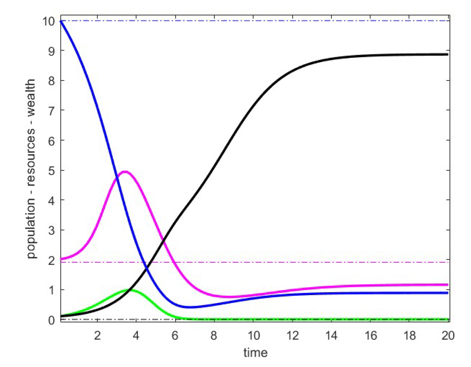
Figure 2.
Case 2: Phase plot for with fixed.
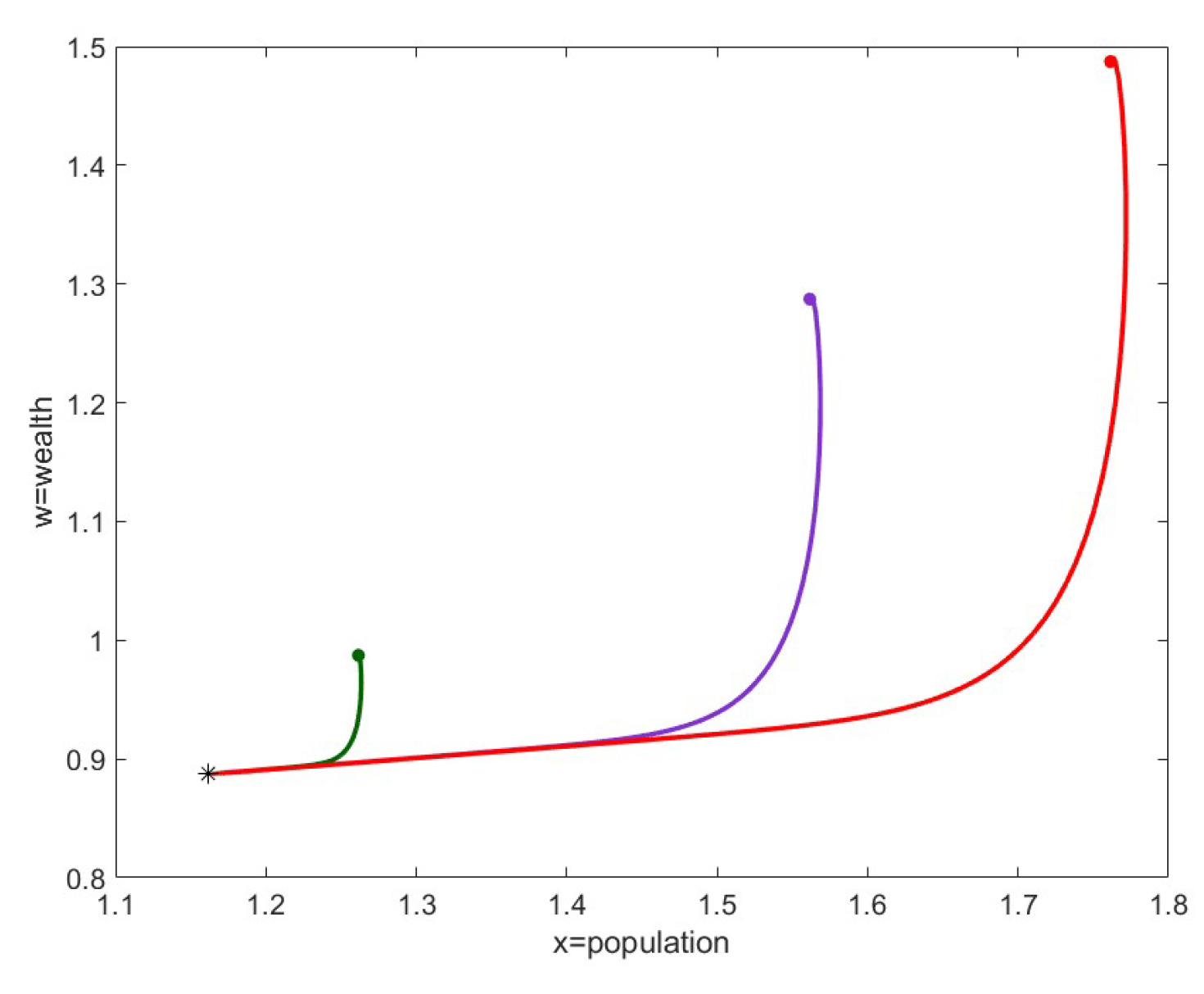
Figure 3.
Case 3: ,

Figure 4.
Case 3: .
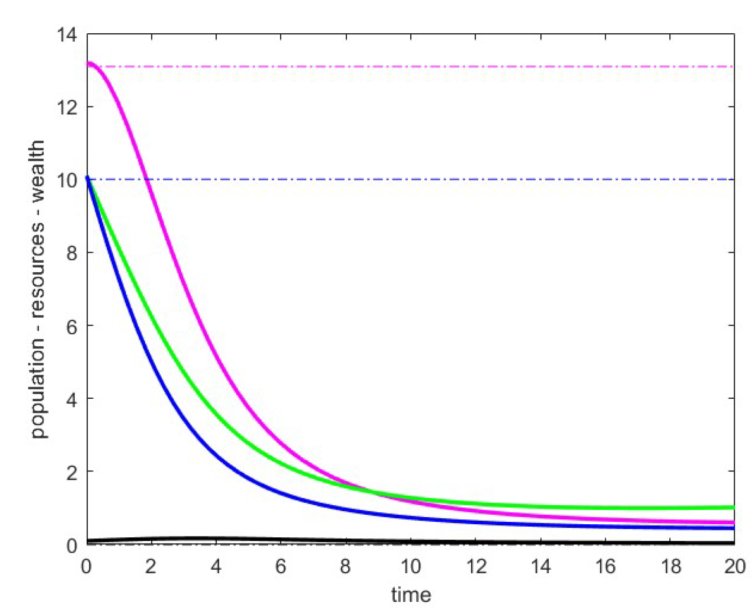
Figure 5.
Case 4: point , phase plot
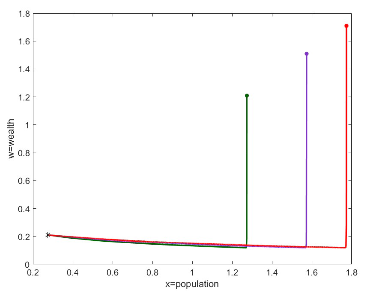
Figure 6.
Case 4: trajectories near .

Disclaimer/Publisher’s Note: The statements, opinions and data contained in all publications are solely those of the individual author(s) and contributor(s) and not of MDPI and/or the editor(s). MDPI and/or the editor(s) disclaim responsibility for any injury to people or property resulting from any ideas, methods, instructions or products referred to in the content. |
© 2025 by the authors. Licensee MDPI, Basel, Switzerland. This article is an open access article distributed under the terms and conditions of the Creative Commons Attribution (CC BY) license (http://creativecommons.org/licenses/by/4.0/).
Copyright: This open access article is published under a Creative Commons CC BY 4.0 license, which permit the free download, distribution, and reuse, provided that the author and preprint are cited in any reuse.


