From Barthel-Randers-Kropina Geometries to the Accelerating Universe: A Brief Review of Recent Advances in Finslerian Cosmology

1. Introduction-Early History and Modern Developments

In 1918, the same year in which Herman Weyl proposed his important extension of Riemannian geometry [1,2], by introducing in mathematics and physics the concept of nonmetricity, another equally interesting generalization of the Riemannian framework was proposed by Paul Finsler [3]. The work of Weyl was clearly influenced by the progresses in the physics of his time, and especially by the development by Einstein [4,5] and Hilbert [6] of general relativity, and has been extensively used in physics, especially recently [7]. On the other hand, Finsler geometry, which represents, at least from a physicist’s perspective, a much more drastic extension of Riemannian geometry, was not considered from the point of view of the applications in fundamental physics for at least 40 years.

Actually, Finslerian geometry was already anticipated by Riemann [8], who has already assumed the existence of metric structures in a general space based on the distance element $ds=F\left(x^1,x^2,\dots ,x^n;d{x}^1,d{x}^2,\dots ,d{x}^n\right)=F\left(x^1,x^2,\dots ,x^n;,y^1,y^2,\dots ,y^n\right)$, or simply $F(x,y)$, where the condition that for $y=0$, F is a positive definite function defined on the tangent bundle $TM$ must also be imposed. In order to assure the independence of the length of curves on their parameterization, it is further required that F is a function which is homogeneous of degree one in y. Riemann geometry is just a special case of the general distance element $ds$, obtained under the assumption $F^2=g_{IJ}\left(x\right)d{x}^{I}d{x}^J$. Thus, Finsler geometry is not a proper generalization of Riemann’s geometry, but it "...is just Riemannian geometry without the quadratic restriction" [9]. However, it is an established practice especially in the physics literature to describe Finsler geometry as a generalization of Riemann’s geometry, and in the present work we will also adopt this view, mostly for the simplicity of the presentation.

In a simple description Finsler geometry can be considered as a geometry in which the metric tensor $g_{ij}$ is a function of both the coordinates x, defined on the base manifold M, and of the tangent vectors y, so that $g_{IJ}=g_{IJ}(x,y)$. In a physically intuitive sense Finsler geometry can be considered as a geometry in which the metric tensor, determining the distance between two neighboring points, is an arbitrary function of both coordinates and velocities. For presentations of Finsler geometry from a mathematical perspective see [10,11,12,13,14].

The remarkable success of general relativity in the description of gravitational phenomena, and its many observational confirmations have significantly strengthened the position of the Riemannian geometry as the "true" geometry of nature. General relativity, in its Riemannian formulation, successfully passes all the Solar System tests, inside which it can explain with a high precision the gravitational phenomenology. Important confirmations of the validity of general relativity include such diverse phenomena as the perihelion precession of Mercury, light bending by the Sun, frame dragging, the Nordtvedt effect in lunar motion, and the Shapiro time delay, respectively [15]. The experimental detection of gravitational waves represents a brilliant confirmation of the predictions of general relativity [16], which opened a new window on the Universe, and led to new perspectives on the black hole properties, their dynamical evolution, and the mass distribution of neutron stars [17]. Inspired by the immense success of general relativity, the Riemannian geometric framework was also extended, leading to important developments in mathematics like the introduction of the concept of torsion [18,19], or of the concept of absolute parallelism [20]. These new geometries have found important applications in physics, and they have been used to model the gravitational interaction from new perspectives.

From a mathematical point of view, Ehlers Pirani and Schild aimed to develop a constructive axiomatization of gravity. In their seminal 1972 paper, they built up the kinematical structure of general relativity, purely based on axioms, which have a somewhat empirical content [21]. Although the axiomatization is quite dense and technical, recent pedagogical reviews are present in the literature [22,23,24]. We briefly outline the four steps of the axiomatization in the following [25]:

• In the first step, the basic physical/empirical entities are postulated, such as the timelike worldlines for freely falling massive particles, the lightlike wordlines of light rays, and radar echoes between massive particle wordlines. These empirical elements provide enough structure to define a system of coordinates and allow for the construction of a differentiable structure on the spacetime set M, turning it into a smooth manifold.
• The conformal structure is established by requiring that, at each point in spacetime, the set of all possible directions (i.e. tangent vectors) splits into two components when the directions corresponding to massless (lightlike) trajectories are removed. This splitting reflects the causal distinction between future and past. Additionally, in a sufficiently small neighborhood V around the worldline of a massive particle, for any point $p\in V$ not lying on the particle’s path, the function that maps p to the product of the radar emission time $t_e$ and reception time $t_a$, i.e. $p\mapsto t_e{t}_r$, must be at least twice differentiable.
• Imposing that through each point in spacetime, and for each timelike direction, there exists one unique timelike (massive) trajectory passing through that point, results in a projective structure. Each of these trajectories must admit a parametrization such that, in local coordinates near the point, the motion satisfies $\ddot{x}=0$. This expresses the fact that particles move along straight lines in free fall.
• In the final step the compatibility between the conformal and projective structures is demanded. In particular, light rays must be special cases of particle geodesics in the limit of zero mass. This determines the metric up to a conformal factor, which leads to a Weyl structure. Through some technical steps (see .), eliminating the second clock effect leads to a Lorentzian structure, i.e. a pseudo-Riemannian manifold.

It turns out that if one weakens the twice differentiability assumption on the map $p\mapsto t_e{t}_r$, there are Finsler functions, which satisfy all the other EPS axioms. A well known example is given by

$$F(x,y)=e^{2\sigma (x,y)}\sqrt{\left|a_{IJ}\left(x\right)y^I{y}^J\right|},$$

(1)

where $\sigma (x,y)$ is a non-singular 0-homogeneous function in y satisfying

$${\partial }_K\sigma -y^M{\Gamma }_{MK}^N\left(x\right){\displaystyle \frac{\partial \sigma (x,y)}{\partial y^N}}=0$$

(2)

with ${\Gamma }_{MK}^N$ being the Christoffel symbols associated to the Riemannian metric $a_{IJ}\left(x\right)$. This geometry is of Berwald type, i.e. it is the closest to a Riemannian geometry, but it is not trivial.

Despite the systematic, rigorous and physically appealing nature of Finsler geometry, the applications in physics of this geometry appeared relatively late. A first step in this direction was taken in the work of Randers [26], who tried to formulate a unified theory of electromagnetism and gravity. Initially, the theory was formulated in a higher dimensional Riemannian geometry. The Finslerian nature of the Randers geometry was recognized by Ingarden [27]. Essentially, Randers geometry is a specific example of a Finsler geometry, with the fundamental function $F(x,y)={\left(a_{IJ}\left(x\right)d{x}^{I}d{x}^J\right)}^{1/2}+b_K\left(x\right)y^K$, where $b_K\left(x\right)$ is an arbitrary vector field. Presently, Randers spaces are considered as Finsler spaces $F^n=(M,\alpha +\beta )$, equipped with the Cartan nonlinear connection N, i.e. they are denoted with $R{F}^n=(M,\alpha +\beta ,N)$ [28]. A comprehensive overview of several Finsler metrics and of some of their physical applications is given in Table 1.

Finsler geometry has found applications in several areas of physics, including the geometric formulation of quantum mechanics [29,30,31,32], kinetic theory of gases [33,34], dispersion relations [35] and optics [36]. A more exotic application is related to an extension of the Standard Model of particle physics, where a Finsler structure can be given for the nonminimal fermion sector [37]. It is also interesting to note that Lorentz-violating scalar fields can also be described by Riemann-Finsler geometry [38]. In the latter cases, the Finsler geometry considered is of Berwald type: the closest one to the Riemannan geometry, which is still not trivial and compatible with the weakened Ehlers-Pirani-Schild axioms.

The first attempts at formulating a Finslerian theory of gravitation, but still in the framework of unified field theories, belonged to Horváth [39], and Horváth and Moór [40]. Early Finslerian type gravitational theories were also formulated in [41,42], respectively, where a set of Finslerian type gravitational field equations were proposed, representing a straightforward extension of the Einstein field equations, and given by

$$R_{\mu \nu }-{\displaystyle \frac{1}{2}}{g}_{\mu \nu }R+\lambda g_{\mu \nu }=\chi T_{\mu \nu },K_{\mu \nu }-{\displaystyle \frac{1}{2}}{g}_{\mu \nu }K+\lambda g_{\mu \nu }=\chi T_{\mu \nu },$$

(3)

and

$$S_{\mu \nu }-{\displaystyle \frac{1}{2}}{g}_{\mu \nu }S-{\lambda }^{\left(i\right)}{g}_{\mu \nu }=-{\chi }^{\left(i\right)}{T}_{\mu \nu }^i,$$

(4)

respectively. In Eqs. (3) and (4) $\chi$ denotes the gravitational constant, $\lambda$ is the cosmological constant, while ${\lambda }^{\left(i\right)}$ and ${\chi }^{\left(i\right)}$ represent the internal cosmological and gravitational constants. The quantities $R_{\mu \nu }$, R, $K_{\mu \nu }$, K and $S_{\mu \nu }$ and S denoting the hh-, hv- and vv-Ricci curvature tensors, and the hh-, hv- and vv-scalar curvatures of the Finsler space $(M,F)$. Moreover, $T_{\mu \nu }$ is the energy-momentum tensor of the baryonic matter, and $T_{\mu \nu }^i$ denotes the internal energy-momentum tensor. In [43] another Finslerian type approach to gravity was introduced and developed. The main focus of this work was the Finslerian description and interpretation of the particle motion in a gravitational field. For the Finslerian extensions of general relativity along the line of [43] see [44]. Finslerian type generalized Schwarzschild metrics have been investigated in [45,46].

Miron [47] has proposed the vector bundle point of view to formulate a system of Einstein type gravitational field equations. The starting point of this approach is to interpret the field y as a fibre at the point x of the base manifold M. The total space of this vector bundle is obtained as a unification of the fields x and y [48]. A nonlinear connection naturally induces an adapted basis in the fiber $T_{(x,y)}TM$ of the double tangent bundle $TTM$ and a corresponding dual basis in the fiber $T_{(x,y)}^{*}TM$ of the cotangent bundle $T^{*}TM$. These are given by

$$X_A=\left({\displaystyle \frac{\delta }{\delta x^{\lambda }}}={\displaystyle \frac{\partial }{\partial x^{\lambda }}}-N_{\lambda }^i{\displaystyle \frac{\partial }{\partial y^i}},{\displaystyle \frac{\partial }{\partial y^i}}\right),X^A=\left(d{x}^{\kappa },\delta y^i=d{y}^i+N_{\lambda }^{i}d{x}^{\lambda }\right),$$

(5)

respectively.

In Eq. (5), the indices $A,B$ run over $\left(\kappa ,i\right)\in \left\{0,1,2,3,...,7\right\}$, while the Greek indices $\lambda ,\kappa$ take values in $\{0,1,2,3\}$. The functions $N_{\lambda }^i$ define the nonlinear connection. By construction, the basis (5) is adapted to a Finsler-type metric on $TM$, given by

$$G=g_{\lambda \kappa }(x,y)d{x}^{\kappa }d{x}^{\lambda }+g_{ij}(x,y)\delta y^i\delta y^j,$$

(6)

where $g_{\lambda k}(x,y)$ and $g_{ij}(x,y)$ are the horizontal and vertical metric components, respectively.

On the total space of the vector bundle the Einstein field equations are assumed to have their standard general relativistic form, ${\mathcal{R}}_{AB}-(1/2)\mathcal{R}{g}_{AB}={\tau }_{AB}$, where ${\tau }_{AB}$ is the matter energy-momentum tensor. The field equations can be decomposed, and can be written down as [47]

$$R_{\lambda \nu }-{\displaystyle \frac{1}{2}}(R+S)g_{\lambda \nu }={\tau }_{\lambda \nu },{\stackrel{1}{P}}_{i\lambda }={\tau }_{i\lambda },{\stackrel{2}{P}}_{\lambda i}=-{\tau }_{\lambda i},$$

(7)

$$S_{ij}-{\displaystyle \frac{1}{2}}(R+S)g_{ij}={\tau }_{ij}.$$

(8)

An interesting Finslerian type gravitational theory was proposed in [49]. The basic idea of this approach is the assumption that the Einstein vacuum field equations can be obtained from the condition $H=H_i^i=0$, where $H_k^i$, the Finslerian deviation tensor, is obtained from the first and second derivatives of the quantity $G^l={\gamma }_{jk}^l{\dot{x}}^j{\dot{x}}^k/2$ as

$$H_k^i=2{\displaystyle \frac{\partial G^i}{\partial x^k}}-{\displaystyle \frac{{\partial }^2{G}^i}{\partial x^j\partial {\dot{x}}^k}}{\dot{x}}^j+2{\displaystyle \frac{{\partial }^2{G}^i}{\partial {\dot{x}}^j\partial {\dot{x}}^k}}{G}^j-{\displaystyle \frac{\partial G^i}{\partial {\dot{x}}^j}}{\displaystyle \frac{\partial G^j}{\partial {\dot{x}}^k}}.$$

(9)

If the metric is Riemannian, we obtain the limiting case of the general relativistic gravitational field equations. But Finslerian solutions of the gravitational field equations proposed in [49] can also be obtained.

An important class of Finsler geometries is represented by the Berwald-Finsler spaces. A system of gravitational field equations defined in a Berwald geometry was proposed and investigated in [50]. The derivation of the field equations in the Berwald-Finsler geometry is essentially based on the Bianchi identities satisfied by the Chern curvature tensor. In general the geometric part of the gravitational field equation is not symmetric, and this indicates that the principle of the local Lorentz invariance is not satisfied in this theory. The field equations as proposed in [50] are given by

$$\begin{array}{c}\hfill \left[Ri{c}_{\mu \nu }-{\displaystyle \frac{1}{2}}{g}_{\mu \nu }S\right]+\left\{{\displaystyle \frac{1}{2}}{B}_{\alpha \mu \nu }^{\alpha }+B_{\mu \nu \alpha }^{\alpha }\right\}=8\pi G{T}_{\mu \nu },\end{array}$$

(10)

where

$$A_{\lambda \mu \nu }\equiv {\displaystyle \frac{F}{4}}{\displaystyle \frac{\partial }{\partial y^{\lambda }}}{\displaystyle \frac{\partial }{\partial y^{\mu }}}{\displaystyle \frac{\partial }{\partial y^{\nu }}}\left(F^2\right),$$

(11)

is the Cartan tensor, and $B_{\mu \nu \alpha \beta }=-A_{\mu \nu \lambda }{R}_{\theta \alpha \beta }^{\lambda }{y}^{\theta }/F$. The Cartan tensor measures the deviation of the Finsler geometry from the Riemannian one on a given manifold.

With the use of a variational principle, Finsler type gravitational field equations have been derived from a Finsler-Lagrange function L in [51]. The action considered in [51] is given by

$$S\left[L\right]={\int }_{\Sigma \subset TM}\mathrm{vol}(\Sigma )R_{|\Sigma },$$

(12)

where $\Sigma =\{(x,\dot{x})\in TM|F(x,\dot{x})=1\}$ denotes the unit tangent bundle, and $\mathrm{vol}(\Sigma )$, the volume form on $\Sigma$, is defined by using the Finsler metric. The field equations obtained from the action (12) are given by

$$2R-{\displaystyle \frac{L}{3}}{g}^{Lij}{R}_{·i·j}+{\displaystyle \frac{2L}{3}}{g}^{Lij}\left[{(\nabla P_i)}_{·j}+P_{i|j}-P_i{P}_j\right]=0,$$

(13)

where P is the Landsberg tensor, and

$$g_{ij}^L={\displaystyle \frac{1}{2}}{\displaystyle \frac{{\partial }^{2}L}{\partial {\dot{x}}^i\partial {\dot{x}}^j}}={\displaystyle \frac{1}{2}}{L}_{·i·j}.$$

(14)

Moreover, $R_{.i.j}$ is the geodesic deviation operator, and R denotes its trace.

When extended to gravitational systems much bigger than the Solar System, which involves the presence of galactic and cosmological scales, Einstein’s theory of general relativity is facing a number of very serious challenges, whose possible solutions could be obtained only if we introduce a fundamental modification in our understanding of the gravitational force.

One of the most intriguing discoveries of the recent times is the observational proof that our Universe is in fact in a phase of accelerating expansion [52,53,54,55,56]. The transition from deceleration to acceleration occurred at a small redshift z, given by $z\approx 0.5$. To explain this observation requires a profound modification of the theoretical foundations of Einstein’s general relativity.

The simplest explanation for the recent, exponential de Sitter type expansion can be obtained by reintroducing in the Einstein field equations the cosmological constant $\Lambda$, introduced by Einstein in 1917 [57], and later rejected by him as the biggest blunder of his life. Einstein’s main goal was to use $\Lambda$ to construct a static, general relativistic cosmological model of the Universe.

The cosmological constant has a complicated history [58], but presently it is adopted as one of the basic physical (geometrical?) parameters to build up the standard cosmological paradigm, the $\Lambda$CDM model, which is currently used for the interpretation of the observational data. The $\Lambda$CDM model also includes in its theoretical structure another basic, equally mysterious, component, the dark matter [59]. Intensive searches for the dark matter particle have yielded no results, and thus the only evidence for the existence of dark matter is gravitational. However, despite these theoretical shortcomings, the $\Lambda$CDM model fits the observational data very well [60,61,62,63].

But on the theoretical level the $\Lambda$CDM model is confronted with the uncertainty of its foundations: no (convincing) physical theory does exist which could provide it with a solid basis. The first major problem is related to the geometrical or physical interpretation of the cosmological constant [58,64,65]. If we interpret the cosmological constant as the vacuum energy density ${\rho }_{vac}$ at the Planck scale, we are led to the “worst prediction in physics” [66]. The vacuum energy density can be computed as

$${\rho }_{vac}\approx {\displaystyle \frac{\hslash }{c}}{\int }_{k_{dS}}^{k_{Pl}}\sqrt{k^2+{\left({\displaystyle \frac{mc}{\hslash }}\right)}^2}{d}^{3}k\approx {\rho }_{Pl}={\displaystyle \frac{c^5}{\hslash G^2}}={10}^{93}{\displaystyle \frac{\mathrm{g}}{{\mathrm{cm}}^3}},$$

(15)

and this result differs by a factor of ${10}^{-120}$ from the observed value of the energy density associated to $\Lambda$, ${\rho }_{\Lambda }=\Lambda c^2/8\pi G\approx {10}^{-30}\mathrm{g}/{\mathrm{cm}}^3$ [67].

Presently, the $\Lambda$CDM standard paradigm is faced with several important problems. An important challenge to the $\Lambda$CDM model is the "Hubble tension", which has its origins in the differences in the estimations of the values of the Hubble constant $H_0$ (representing the present day value of the Hubble function H), obtained on one hand from the CMB measurements [68], and on the other hand from the local observations of the Type Ia supernovae [69,70,71]. The value of $H_0$ obtained by the SHOES collaboration for $H_0$ is $H_0=74.03\pm 1.42$ km/s/Mpc [69]. The early Universe determinations, using the Planck satellite data, give for $H_0$ the value $H_0=67.4\pm 0.5$ km/s/Mpc [68], which differs by $\sim 5\sigma$ from the SH0ES estimations.

Several other theoretical problems whose solution cannot be found in the framework of the $\Lambda$CDM paradigm still exist. Some of these problems are represented by the question of the smallness of $\Lambda$ and its fine tuning. The question of why the transition from the decelerating to the accelerating phases took place recently is still waiting for a response. And perhaps the most important question, if the cosmological constant is really required to construct successful cosmological models, does not have an answer yet.

Hence, considering alternative approaches for the description of the gravitational interaction may allow us to solve the observational problems of cosmology the consideration of the cosmological constant. There are three major possibilities that have been proposed for the extension of general relativity, the dark components approach, the dark gravity approach, and the dark coupling approach [72]. In the dark gravity approach it is assumed that the geometry of the Universe, as well as the description of the gravitational interaction requires a significant departure from the formalism of the Riemann geometry. Geometries that go beyond the Riemannian one, like, for example, Weyl geometry, geometries with torsion, or teleparallel geometries have been investigated in [73,74,75,76,77,78,79,80,81,82,83]. For reviews of dark gravity type theories, and of their applications, see [84,85,86,87,88].

As a dark gravity candidate, Finsler geometry has an important scientific potential yet to be explored, despite the fact that it has already been considered in various contexts as an important alternative to Riemann geometry, and the standard $\Lambda$CDM paradigm.

Randers geometry was extensively applied in the study of the gravitational phenomena in [89,90,91,92,93,94,95,96,97,98,99,100,101,102,103,104,105,106,107,108,109]. In [93], generalized Friedmann equations in a Randers-Finsler geometry of the form

$$\dot{H}+H^2+{\displaystyle \frac{3}{4}}H{Z}_t=-{\displaystyle \frac{4\pi G}{3}}\left(\rho +3p\right),$$

(16)

$$\dot{H}+3H^2+{\displaystyle \frac{11}{4}}H{Z}_t=4\pi G\left(\rho -p\right),$$

(17)

have been obtained, where H, $\rho$, p are the Hubble function, and the baryonic matter energy density and pressure, respectively. The quantity $Z_t={\dot{u}}_0$, with $u_0$ denoting the time component of the four-velocity $u_{\mu }$. The generalized Friedmann equations above give the relation $3H^2+3H{Z}_t=8\pi G\rho$. The term $H{Z}_t$, induced by the Finsler-Randers geometry, leads to the existence of new phases in the cosmic evolution of the Universe. The system of Friedmann equations (16) and (17) were used in [94] for the investigation of particle creation processes in the Finsler type geometries.

A scalar-tensor theory that arises effectively from the Lorentz fiber bundle of a Finsler-type geometry was proposed in [110], where its cosmological implications were also investigated. The action in the presence of matter considered in this work is

$$\mathcal{S}={\displaystyle \frac{1}{16\pi G}}\int \sqrt{|det\mathbf{G}|}{\mathcal{L}}_{G}d{x}^{\left(N\right)}+\int \sqrt{|det\mathbf{G}|}{\mathcal{L}}_{M}d{x}^{\left(N\right)},$$

(18)

where $d{x}^{\left(N\right)}=d^{4}x\wedge {\varphi }^{\left(1\right)}\wedge {\varphi }^{\left(2\right)}$. Several Lagrangian densities were adopted, given by

$${\mathcal{L}}_G=\tilde{\mathcal{R}}-{\displaystyle \frac{1}{\varphi }}V\left(\varphi \right),$$

(19)

where $V\left(\varphi \right)$ is the potential for the scalar $\varphi$, and

$$\tilde{\mathcal{R}}=R-{\displaystyle \frac{2}{\varphi }}\square \varphi +{\displaystyle \frac{1}{2{\varphi }^2}}{\partial }_{\mu }\varphi {\partial }^{\mu }\varphi ,$$

(20)

where $\tilde{\mathcal{R}}$ denotes the curvature for the particular situation of a holonomic basis $[X_M,X_N]=0$. In the case of a non-holonomic basis the adopted Lagrangian density is given by ${\overline{\mathcal{L}}}_G=\tilde{R}$. The generalized Friedmann equations are given by

$$\begin{array}{cc}\hfill & 3H^2=8\pi G{\rho }_m-{\displaystyle \frac{{\dot{\varphi }}^2}{4{\varphi }^2}}+{\displaystyle \frac{1}{\varphi }}\left({\displaystyle \frac{V\left(\varphi \right)}{2}}-3H\dot{\varphi }\right),\hfill \end{array}$$

(21)

$$\begin{array}{cc}\hfill & \dot{H}=-4\pi G({\rho }_m+P_m)+{\displaystyle \frac{{\dot{\varphi }}^2}{4{\varphi }^2}}+{\displaystyle \frac{1}{2\varphi }}\left(H\dot{\varphi }-\ddot{\varphi }\right),\hfill \end{array}$$

(22)

$$\ddot{\varphi }+3H\dot{\varphi }=-16\pi G\varphi {\rho }_m-6\varphi \left(\dot{H}+2H^2\right)+\varphi V^{\prime }\left(\varphi \right)+{\displaystyle \frac{{\dot{\varphi }}^2}{2\varphi }},$$

(23)

and

$$\begin{array}{ccc}& & 3H^2=8\pi G{\rho }_m-(1+A){\displaystyle \frac{{\dot{\varphi }}^2}{4{\varphi }^2}}-3H{\displaystyle \frac{\dot{\varphi }}{\varphi }},\hfill \end{array}$$

(24)

$$\begin{array}{ccc}& & \dot{H}=-4\pi G({\rho }_m+P_m)+(1+A){\displaystyle \frac{{\dot{\varphi }}^2}{4{\varphi }^2}}+{\displaystyle \frac{1}{2\varphi }}\left(H\dot{\varphi }-\ddot{\varphi }\right),\hfill \end{array}$$

(25)

$$\begin{array}{ccc}& & (1+A)\left(\ddot{\varphi }+3H\dot{\varphi }\right)=-16\pi G\varphi {\rho }_m-6\varphi \left(\dot{H}+2H^2\right)+{\displaystyle \frac{{\dot{\varphi }}^2}{2\varphi }}\left(1+A+\varphi A^{\prime }\right)-\dot{\varphi }\dot{A},\hfill \end{array}$$

(26)

respectively. Here $A\left(\varphi \right)$ denotes a real function of $\varphi$. From the above equations one can reconstruct the thermal history of the Universe, and obtain a sequence of matter and dark-energy dominated phases. The effective dark energy equation of state has a parameter that can be either phantom or quintessence type. A phantom-divide crossing during the cosmological evolution does also appear.

Berwald-Finsler geometries have been investigated as potential candidates for the description of the gravitational fields [111,112]. Spatially homogeneous and isotropic Berwald spacetimes, obtained from a Finsler Lagrangian constructed from a zero-homogeneous function defined on the tangent bundle, and which includes the velocity dependence of the Finsler Lagrangian, were discussed in [112]. Cosmological Berwald geometries can also be used for the description of the dynamics of the Universe.

In a series of recent papers [113,114,115,116] a systematic investigation of the applications of Finsler geometry in cosmology was considered. The basic geometric ingredients used for the construction of gravitational theories were the $(\alpha ,\beta )$ metrics, and the osculating Barthel connection. One of the basic properties of the Finsler geometry is that to each point of the space-time manifold an arbitrary point vector field y is associated, with the metric g becoming a function of both x, the coordinates defined on the base manifold, and y, $g=g(x,y)$. In the osculating approach one assumes the existence of a vector field $Y=Y\left(x\right)$, which allows the construction of a Riemannian metric $g\left(x\right)=g(x,Y(x\left)\right)$. In the case of the $(\alpha ,\beta )$ metrics, the connection associated to these metrics, the Barthel connection, is nothing but the Levi-Civita connection associated to $g\left(x\right)$.

The introduction in the $(\alpha ,\beta )$ spaces of the Finsler geometry of the osculating Barthel connection leads to a significant simplification of the mathematical formalism, and opens the possibility of constructing unique and well defined physical models that could be successfully used for the description of the gravitational interaction. In the present review we briefly introduce, from the perspective of the cosmological applications, the Barthel-Randers, Barthel-Kropina, and the conformal Barthel-Kropina models, respectively, and we also present their mathematical and theoretical foundations.

From the generalized Friedmann equations of the osculating Barthel–Randers-Kropina cosmological models, obtained by assuming that the background Riemannian metric is of the Friedmann–Lemaitre–Robertson–Walker (FLRW) type, an effective geometric dark energy component can be always generated, which results from the presence of extra terms in the cosmological evolution equations.

A central problem for the physical acceptability of the Finslerian type models is how successfully could they describe the observational data. The cosmological tests, and comparisons with observational data of theis dark energy models considered in this work are investigated are considered in detail. In the present review we perform a detailed analysis of the three cosmological models of Barthel-Randers type, introduced in [113], we constrain the model parameters. In our investigation we use 15 Hubble data points (Cosmic Chronometers), the Pantheon Supernovae Type Ia data sample, and the most recent Baryon Acoustic Oscillation (BAO) measurements from the Dark Energy Spectroscopic Instrument (DESI) Data Release 2. The statistical analysis is performed by using Markov Chain Monte Carlo (MCMC) simulations. The results of the statistical analysis of the Barthel-Randers cosmological models are compared with the similar analysis of the Barthel-Kropina cosmological models, already performed in [115], and with the standard $\Lambda$CDM model. The Akaike information criterion (AIC), and the Bayesian information criterion (BIC) are used as the models selection tools. The statefinder diagnostics, consisting in the study of the jerk and snap parameters, and the $Om\left(z\right)$ diagnostics are also considered for the comparative study of the Barthel-Randers, Barthel–Kropina and $\Lambda$CDM cosmologies. Our statistical results indicate that the osculating Barthel type $(\alpha ,\beta )$ Finslerian dark energy models give a good description of the observational data, and thus they can be considered a viable alternative of the $\Lambda$CDM model, even if not all of them would be favoured compared to $\Lambda$CDM.

The present paper is organized as follows. We review some basic concepts and definitions of Finsler geometry in Section 2. In Section 3 we introduce the mathematical foundations of the Barthel-Randers-Kropina gravitational theories, by reviewing the basic concepts of $(\alpha ,\beta )$ metrics, osculating spaces, and Barthel connections. The basic principles of constructing $(\alpha ,\beta )$ cosmological models are also presented. The generalized Friedmann equations of the three basic models considered in the present work: Barthel-Randers, Barthel-Kropina and conformal Barthel-Kropina are also written down, together with the corresponding energy balance equations. The thermodynamic interpretation of the cosmological models with nonvanishing matter energy-momentum tensor is also presented, and briefly discussed. The cosmological implications of the Barthel-Randers and Barthel-Kropina models are discussed in Section 4, where constraints on the free parameters of these models are obtained by using a combination of observational data sets, including Type Ia supernovae, Baryon Acoustic Oscillations, and Hubble parameter measurements. A detailed comparison of the Barthel-Randers and Barthel-Kropina cosmological models is performed in Section 5. A discussion of the main results and of the relevance of the statistical analysis is presented in Section 6. Finally, we discuss and conclude our results in Section 7.

2. Fundamentals of Finsler Geometry

The assumption that spacetime can be described mathematically as a four dimensional differentiable manifold M, endowed with a pseudo-Riemannian tensor $g_{IJ}$, where $I,J,K...=0,1,2,3$, is one of the fundamental assumptions of modern theoretical physics. The next fundamental concept, the interval between two events located at the points $x^I$ and $x^I+d{x}^I$ on the world line of a standard clock is defined by the chronological hypothesis as $ds={\left(g_{IJ}d{x}^{I}d{x}^J\right)}^{1/2}$ [117,118]. A very important metrical generalization of the Riemannian geometry is the geometry anticipated by Riemann [8], but which was later on systematically developed by Finsler [3].

In a simple interpretation Finsler spaces are metric spaces with the interval $ds$ between two neighboring points $x=\left(x^I\right)$ and $x+dx=(x^I+d{x}^I)$ given by

$$ds=F\left(x,dx\right),$$

(27)

where F, the Finsler metric function, must be positively homogeneous of degree one in $dx$, and thus satisfy the condition

$$F\left(x,\lambda dx\right)=\lambda F\left(x,dx\right)\mathrm{for}\lambda >0.$$

(28)

The Finsler metric function F can be written in terms of the canonical coordinates of the tangent bundle $(x,y)=(x^I,y^I)$, where $y=y^I\left(\partial /\partial x^I\right)$, is any tangent vector y at x. Then we can introduce the Finsler metric tensor $g_{IJ}$ defined according to

$$g_{IJ}\left(x,y\right)={\displaystyle \frac{1}{2}}{\displaystyle \frac{{\partial }^2{F}^2\left(x,y\right)}{\partial y^I\partial y^J}}.$$

(29)

Hence Eq. (27) can be written as

$$d{s}^2=g_{IJ}\left(x,y\right)y^I{y}^J.$$

(30)

Riemann spaces are some particular cases of the Finsler spaces, and they correspond to $g_{IJ}\left(x,y\right)=g_{IJ}\left(x\right)$ and $y^I=d{x}^I$, respectively.

Given a Finsler function F, one can obtain the geodesic equations in the form [117,118]

$${\displaystyle \frac{d^2{x}^I}{d{\lambda }^2}}+2G^I\left(x,y\right)=0,$$

(31)

where the functions $G^i(x,y)$ denote the spray coefficients

$$G^I\left(x,y\right)={\displaystyle \frac{1}{4}}{g}^{IJ}\left({\displaystyle \frac{{\partial }^2{F}^2}{\partial x^K\partial y^J}}{y}^K-{\displaystyle \frac{\partial F^2}{\partial x^J}}\right).$$

(32)

Equivalently, more reminiscent to Riemannian geometry, they can be rewritten as

$${\displaystyle \frac{d^2{x}^I}{d{\lambda }^2}}+{\Gamma }_{JK}^I\left(x,y\right){\displaystyle \frac{d{x}^J}{d\lambda }}{\displaystyle \frac{d{x}^K}{d\lambda }}=0,$$

(33)

where

$${\Gamma }_{JK}^I(x,y)y^J{y}^K=2G^i(x,y)={\displaystyle \frac{1}{4}}{g}^{IJ}\left({\displaystyle \frac{{\partial }^2{F}^2}{\partial x^K\partial y^J}}{y}^K-{\displaystyle \frac{\partial F^2}{\partial x^J}}\right).$$

(34)

Here, the quantities ${\Gamma }_{JK}^I(x,y)$ are the local coefficients of the Finsler connection used. We point out that the theory of Finsler connections is more complex than in the Riemannian case since only metrical, torsion free connection is the Levi-Civita one, hence the existence of such connection implies that the Finsler metric is in fact Riemannian. The obvious conditions imposed for the existence of Finsler connections are then non-metricity and torsion free (this is the case of the Chern connection) or metrical connection with surviving torsion (this is the case of the Cartan connection). The precise form of the Finsler connections depends on the concrete form of the non-metricity and surviving torsion, respectively, but these details are beyond the aim of the present paper (one can consult [13,14,127] or other textbooks on Finsler geometry). The local coefficients of a Finsler connection D are defined as

$$D_{{\displaystyle \frac{\delta }{\delta x^K}}}{\displaystyle \frac{\delta }{\delta x^J}}={\Gamma }^I{(x,y)}_{JK}{\displaystyle \frac{\delta }{\delta x^I}},D_{{\displaystyle \frac{\partial }{\partial x^K}}}{\displaystyle \frac{\partial }{\partial x^J}}=V^I{(x,y)}_{JK}{\displaystyle \frac{\partial }{\partial x^I}},$$

(35)

where ${\displaystyle \frac{\delta }{\delta x^I}}$ is the adapted basis induced by the Cartan nonlinear connection. We prefer to keep the notation $C_{JK}^I={\displaystyle \frac{1}{2}}{\displaystyle \frac{{\partial }^3{F}^2}{\partial y^I\partial y^J\partial y^K}}$ for the Cartan tensor of $(M,F)$. For instance, the Cartan connection of a Finsler space $(M,F)$ is the only Finsler connection on $TTM$ which is metrical and having $h\left(hh\right)$ and $v\left(vv\right)$-torsion vanishing (the rest of the torsion survives). The local coefficients of the Cartan connection are given by

$$\begin{array}{cc}\hfill {\Gamma }_{JK}^I\left(x,y\right)& ={\displaystyle \frac{1}{2}}{g}^{IL}\left(x,y\right)\left[{\displaystyle \frac{\delta g_{LJ}\left(x,y\right)}{\delta x^K}}+{\displaystyle \frac{\delta g_{LK}\left(x,y\right)}{\delta x^J}}-{\displaystyle \frac{\delta g_{JK}\left(x,y\right)}{\delta x^L}}\right]\hfill \\ \hfill V_{JK}^I\left(x,y\right)& ={\displaystyle \frac{1}{2}}{g}^{IL}\left(x,y\right)\left[{\displaystyle \frac{\partial g_{LJ}\left(x,y\right)}{\partial y^K}}+{\displaystyle \frac{\partial g_{LK}\left(x,y\right)}{\partial y^J}}-{\displaystyle \frac{\partial g_{JK}\left(x,y\right)}{\partial x^L}}\right],\hfill \end{array}$$

(36)

Likewise, the Chern connection is defined to be the only Finsler connection on $TTM$ which is almost compatible and torsion free. The local coefficients of the Cartan connection are given by $({\Gamma }_{JK}^I(x,y),0)$. However, despite the quite complicated form of the connection coefficients ${\Gamma }_{JK}^I(x,y)$, due to the homogeneity of the geometrical objects involved, the equation (33) gets the simple form

$${\displaystyle \frac{d^2{x}^I}{d{\lambda }^2}}+{\gamma }_{JK}^I\left(x,y\right){\displaystyle \frac{d{x}^J}{d\lambda }}{\displaystyle \frac{d{x}^K}{d\lambda }}=0,$$

(37)

where

$$\begin{array}{c}\hfill {\gamma }_{JK}^I\left(x,y\right)={\displaystyle \frac{1}{2}}{g}^{IL}\left(x,y\right)\left[{\displaystyle \frac{\partial g_{LJ}\left(x,y\right)}{\partial x^K}}+{\displaystyle \frac{\partial g_{LK}\left(x,y\right)}{\partial x^J}}-{\displaystyle \frac{\partial g_{JK}\left(x,y\right)}{\partial x^L}}\right].\end{array}$$

(38)

are the formal Christoffel coefficients of the Finsler space $(M,F)$.

Berwald spaces are a special class of Finsler geometry, and they can be obtained by assuming that the Berwald connection coefficients are independent of the fiber coordinate y [10].

With the help of the spray coefficients $G^I$, one can define the vector field S on $TM\setminus 0$ according to

$$S=y^I{\displaystyle \frac{\partial }{\partial x^I}}-2G^I{\displaystyle \frac{\partial }{\partial y^I}}.$$

S is the spray induced by F. A curve $\gamma$ defined on M is a geodesic of F if and only if its canonical lift $\widehat{\gamma }\left(t\right)=(\gamma \left(t\right),\dot{\gamma }\left(t\right))$ to $TM$ is an integral curve of S.

The notion of Finsler metrics that we have recalled here belong to the class of classic Finsler metrics, in other words, at each point $x\in M$, the function $F_x:T_{x}M\to \mathbb{R}$ is a function defined on the tangent space $T_{x}M$ of a differentiable manifold M satisfying the following conditions

(i)

$F_x$ is $C^{\infty }$ on $\widetilde{T_{x}M}=T_{x}M\setminus \left\{0\right\}$,

(ii)

$F_x$ is 1-positive homogeneous: $F_x\left(\lambda y\right)=\lambda F_x\left(y\right)$, for all $\lambda >0$ and $y\in T_{x}M$,

(iii)

for each $x\in M$, the Hessian matrix (29) is positive defined in $\widetilde{T_{x}M}$.

At each point $x\in M$, the indicatrix $\{y\in T_{x}M:F_x\left(y\right)=1\}$ is a closed, strictly convex, smooth hypersurface around the origin of $T_{x}M$.

A more general notion is the notion of conic Finsler metrics, that is, Finsler norms defined only on a conic domain of $T_{x}M$. Let us recall that $A_x\subset T_{x}M$ is called a conic domain of $T_{x}M$ if $A_x$ is an open, non-empty subset of $T_{x}M$ such that if $v\in A_x$, then $\lambda v\in A_x$, for all $\lambda >0$. We remark that the origin of $T_{x}M$ does not belong to $A_x$ except for the case $A_x=T_{x}M$.

We can now define a Finsler norm defined only on a conic domain $A_x\subset T_{x}M$ with the properties (i)-(iii) given above for all $y\in A_x$. At each point $x\in M$, the indicatrix $S_x:=\{y\in A_x\subset T_{x}M:F_x\left(y\right)=1\}$ is a hypersurface embedded in $A_x$ as a closed subset.

Let $A\subset TM$ be an open subset of the tangent bundle $\pi :TM\to M$ such that $\pi \left(A\right)=M$, and A is conic in $TM$, that is for each $x\in M$, the set $A_x:=A\cap T_{x}M$ is a conic domain in $T_{x}M$. A function $F:A\to \mathbb{R}$ is a conic Finsler metric if its restriction $F_x:A_x\to \mathbb{R}$ satisfies the conditions (i)-(iii) above, for each $x\in M$. The local and global geometry of conic Finsler spaces can be now developed in a similar way with the case of classical Finsler metrics (see [119,120] and references therein).

3. Osculating $(\mathbf{\alpha },\mathbf{\beta })$ Type Cosmological Models

In the present Section we review the mathematical and theoretical foundations of the Barthel-Randers-Kropina type cosmological models, which we will discuss in the framework of the general $(\alpha ,\beta )$ geometries. We also write down the generalized Friedmann equations obtained for the case of the Friedmann-Lemaitre-Robertson-Walker Riemannian metric. The thermodynamic interpretation of the models is also discussed.

3.1. Mathematical Foundations of the $(\alpha ,\beta )$ Finslerian Cosmologies

We begin our discussion of the cosmology of the Finslerian type geometries with a brief discussion of the mathematical properties of the $(\alpha ,\beta )$ metrics, of the Barthel connection, and of the osculating geometries.

3.1.1. Kropina and $(\alpha ,\beta )$ Geometries

As we have already mentioned, a special type of Finsler space is the Randers space [26], with the metric function given by

$$F={\left[a_{IJ}\left(x\right)y^I{y}^J\right]}^{1/2}+b_I\left(x\right)y^I,$$

(39)

where $a_{IJ}$ is the metric tensor of a Riemannian space, and $b_I\left(x\right)y^I$ is a linear 1-form defined on the tangent bundle $TM$ and we used the parametrization $d{x}^I=y^I$.

Another remarkable class of Finsler spaces are the Kropina spaces [121,122], which are Finsler spaces with metrics of the form

$$F\left(x,y\right)={\displaystyle \frac{a_{IJ}\left(x\right)y^I{y}^J}{b_I\left(x\right)y^I}}.$$

(40)

By generalizing these results, Matsumoto [123,124] defined the notion of the $(\alpha ,\beta )$ metrics in the following way: being given a Finsler metric function $F(x,y)$, it is called an $(\alpha ,\beta )$ metric if F is a positively homogeneous function $F(\alpha ,\beta )$ of first degree in two variables $\alpha \left(x,y\right)={\left[a_{IJ}\left(x\right)y^I{y}^J\right]}^{1/2}$ and $\beta \left(x,y\right)=b_I\left(x\right)y^I$, respectively.

In our analysis we suppose that $\alpha$ is a pseudo-Riemannian or Riemannian metric, with the properties that it is non-degenerate (regular), or positive-definite, respectively. We point out that the Kropina-type metrics are conic Finsler metrics defined only on some conic domain of the tangent bundle. By extension, we can regard any $(\alpha ,\beta )$ as conic Finsler metrics allowing the Riemannian part to be pseudo-Riemannian metrc.

In the special cases of the Randers and Kropina metrics the Finsler metric functions are given by $F=\alpha +\beta$, and $F={\displaystyle \frac{{\alpha }^2}{\beta }}$, respectively (see also Table 1). Therefore the Randers and Kropina metrics belong to the general class of the $(\alpha ,\beta )$ metrics.

We can define the general $(\alpha ,\beta )$ metrics as metrics having the metric function given by

$$F(\alpha ,\beta )=\alpha \varphi \left(\beta /\alpha \right)=\alpha \varphi \left(s\right),$$

(41)

where $s=\beta /\alpha$, and $\varphi =\varphi \left(s\right)$ is a $C^{\infty }$ positive function on an open interval $(-b_o,b_o)$.

Many examples of $(\alpha ,\beta )$ metrics have been considered in the literature, the most studied one being the Randers metric $F=\alpha +\beta$ (see [125] and references within). The Kropina metrics are also classic examples of $(\alpha ,\beta )$ metrics (see [126] for physical motivations of introducing this metric). More recently, the local and global aspects of Kropina metrics have been extensively studied in [120,128,129,130,131].

3.1.2. The Barthel Connection

Let $(M^n,F)$ be a Finsler space, defined on a base manifold $M^n$. We can also define on $M^n$ a vector field $Y\left(x\right)\ne 0$. We introduce now a specific mathematical object $(M^n,F(x,y),Y\left(x\right))$, which represents a Finsler space $(M^n,F(x,y))$ with a tangent vector field $Y\left(x\right)$ also defined. If the vector Y does not vanish in any point on M, then from the Finslerian metric $\widehat{g}(x,y)$ one obtains the Y-Riemann metric ${\widehat{g}}_Y\left(x\right)=\widehat{g}(x,Y)$.

Obviously, one can evaluate any geometrical object in a Finsler space $(M,F)$ in the specific direction given by a fixed vector field Y. This remark leads to the natural idea of evaluating the Cartan connection coefficients ${\Gamma }_{JK}^I(x,y)$ given in (36) at $y=Y\left(x\right)$. This is the so-called Barthel connection introduced by Barthel himself in [132,133] and developed later by Ingarden and Matsumoto [126].

The Barthel connection is an affine connection on M, ${\widehat{g}}_Y$ metrical with torsion

$$T_{JK}^I\left(x\right)=V_{LJ}^I(x,Y\left(x\right))Y_K^L-V_{LK}^I(x,Y\left(x\right))Y_J^L,$$

(42)

where $Y_J^L\left(x\right):={\displaystyle \frac{\partial Y^L}{\partial x^J}}-N_J^L(x,Y\left(x\right))$ and $N_J^L(x,y)$ is the Cartan nonlinear connection of the Finsler space $(M,F)$.

The local coefficients of the Barthel connection can be written as

$$b_{JK}^I\left(x\right)=F_{JK}^I(x,Y\left(x\right))+V_{JL}^I(x,Y\left(x\right))Y_J^L\left(x\right).$$

(43)

The absolute differential of the vector Y is defined according to [134]

$$D{Y}^I=d{Y}^I+Y^K{b}_{KH}^I(x,Y)d{x}^H,$$

(44)

where by $b_{KH}^I(x,Y)$ we have denoted the coefficients of the Barthel connection. By using the homogeneity of the geometrical objects involved, it results

$$D{Y}^I=d{Y}^I+Y^K\left({\widehat{\gamma }}_{KH}^I-{\widehat{\gamma }}_{KS}^R{Y}^S{\widehat{C}}_{RH}^I\right)d{x}^H,$$

(45)

The Barthel connection has a number of interesting properties. It depends on the vector field on which it acts, a property that does not exist in Riemann geometry. Therefore, the Barthel connection has very different properties, and so it significantly differs from the connections in Riemann geometry. Another important property is related to the direction and magnitude dependence of the Barthel connection. For anisotropic metrics, like most of the Finsler metrics, all geometric properties depend on the direction. For the Barthel connection, there is no dependence on the magnitude of the vector field, but only on its direction. The Barthel connection, keeping the metric function unchanged by the parallel transport, is the simplest connection with this property. For Finsler vector fields, depending on both x and y, the Barthel connection allows the transition to the Cartan geometry of the Finsler spaces. Moreover, the Barthel connection can be considered as the connection of a point Finsler space.

Finally, we would like to mention that unlike the Levi-Civita connection of the Riemannian geometry, the Finsler connections (Cartan or Chern connections) are not defined on the base manifold M, but they live on the total space of the tangent bundle [13,14]. On the other hand, even though they are completely different, the Barthel and Levi-Civita connections are affine connections on the base manifold M. This is a very important characteristic of the Barthel type geometries that leads to significant differences between the geometrical theories of gravity as formulated on Riemann and Finsler manifolds.

3.1.3. The Y-Osculating Riemann Geometry

In 1936 Nazim [135] introduced and developed the concept of osculating Riemann spaces of Finsler geometries. This concept was later studied by Varga [136]. In the osculating approach one associates to a complex geometric object, like a Finsler geometry and connection, a simpler mathematical structure, like, for example, an affine or a linear connection, or a Riemann metric. Hence in this approach it is assumed that the osculating geometry, approximates at a certain level the more complicated one. Thus, with the use of the osculating formalism, one can derive mathematical results that significantly simplifies the description of the properties of the mathematically complex geometries.

Let a nowhere vanishing local section Y of ${\pi }_M:TM\to M$ be given. Geometric objects existing on $TM$ can be pulled back to M. Since $g_{IJ}\circ Y$ is a function defined on U, a new metric, defined according to

$${\widehat{g}}_{IJ}\left(x\right):=g_{IJ}{(x,y)|}_{y=Y\left(x\right)},x\in U,$$

(46)

can be introduced. The pair $\left(U,{\widehat{g}}_{IJ}\right)$ represents a Riemannian manifold, while ${\widehat{g}}_{IJ}\left(x\right)$ is the Y- osculating Riemannian metric, defined on $(M,F)$.

For the osculating Riemannian metric given by Eq. (46), we define the Christoffel symbols of the first kind as

$$\begin{array}{c}\hfill {\widehat{\gamma }}_{IJK}\left(x\right):={\displaystyle \frac{1}{2}}\left\{{\displaystyle \frac{\partial }{\partial x^J}}\left[g_{IK}(x,Y\left(x\right))\right]+{\displaystyle \frac{\partial }{\partial x^K}}\left[g_{IJ}(x,Y\left(x\right))\right]-{\displaystyle \frac{\partial }{\partial x^I}}\left[g_{JK}(x,Y\left(X\right))\right]\right\}.\end{array}$$

(47)

With the use of the rule of the derivative of the composed functions, we explicitly find

$${\widehat{\gamma }}_{IJK}\left(x\right)={\left.{\gamma }_{IJK}(x,y)\right|}_{y=Y\left(x\right)}+2{\left.\left(C_{IJL}{\displaystyle \frac{\partial Y^L}{\partial x^K}}+C_{IKL}{\displaystyle \frac{\partial Y^L}{\partial x^J}}-C_{JKL}{\displaystyle \frac{\partial Y^L}{\partial x^I}}\right)\right|}_{y=Y\left(x\right)},$$

(48)

where $C_{IJL}$ denotes the Cartan tensor. Hence, if a global section Y of $TM$ does exist, so that $Y\left(x\right)\ne 0$, $\forall x\in M$, one can always define the osculating Riemannian manifold $(M,{\widehat{g}}_{ij})$.

The Case of the $(\alpha ,\beta )$ Metrics

Let’s focus now on the case of the $(\alpha ,\beta )$ metrics. The Hessian matrix of an $(\alpha ,\beta )$-metric $F=F(\alpha ,\beta )$ is given by

$$g_{IJ}(x,y)={\displaystyle \frac{L_{\alpha }}{\alpha }}{h}_{IJ}+{\displaystyle \frac{\partial L_{\alpha \alpha }}{{\alpha }^2}}{y}_I{y}_J+{\displaystyle \frac{\partial L_{\alpha \beta }}{\alpha }}\left(y_I{b}_J+y_J{b}_i\right)+L_{\beta \beta }{b}_I{b}_J,$$

(49)

and the Cartan tensor by

$$2C_{IJK}={\displaystyle \frac{L_{\alpha \beta }}{\alpha }}\left(h_{IJ}{p}_K+h_{JK}{p}_I+h_{KI}{p}_J\right)+L_{\beta \beta \beta }{p}_I{p}_J{p}_K,$$

(50)

where the notation $L:={\displaystyle \frac{F^2}{2}}$ is customary. Here $p_I=b_I-{\displaystyle \frac{\beta }{\alpha }}{y}_I$ and $h_{IJ}=g_{IJ}-{\displaystyle \frac{y_I{y}_J}{F^2}}$ is the angular tensor of $(M,F)$.

We choose the vector field as $Y=b$, with $b^I=a^{IJ}{b}_J$. Since the vector field Y is globally non-vanishing on M, we obtain the result that $\beta$ has no zero points on M. Hence, we can define for the $(\alpha ,\beta )$ metrics the b- osculating Riemannian manifold $(M,{\widehat{g}}_{IJ})$, with the Riemannian metric given by ${\widehat{g}}_{IJ}\left(x\right):=g_{IJ}(x,b)$, where $b^I=a^{IJ}{b}_J$.

With respect to $\alpha$, the length $\tilde{b}$ of b is obtained as ${\tilde{b}}^2=b_I{b}^I={\alpha }^2\left(x,b\right)$. Moreover, we have $Y_I\left(x,b\right)=b_I$, respectively.

The b-osculating Riemannian metric can be explicitly written as

$$\begin{array}{c}\hfill {\widehat{g}}_{IJ}\left(x\right)={\left.{\displaystyle \frac{L_{\alpha }}{\tilde{b}}}\right|}_{y=b\left(x\right)}{g}_{IJ}+{\left.\left({\displaystyle \frac{L_{\alpha \alpha }}{{\tilde{b}}^2}}+2{\displaystyle \frac{L_{\alpha \beta }}{\tilde{b}}}+L_{\beta \beta }-{\displaystyle \frac{L_{\alpha }}{{\tilde{b}}^3}}\right)\right|}_{y=b\left(x\right)}{b}_I{b}_J.\end{array}$$

(51)

Moreover, we obtain $\beta \left(x,b\right)={\tilde{b}}^2$, and $p_I\left(x,b\right)=0$. Hence, by using the expression of the Cartan tensor for an $(\alpha ,\beta )$ metric, we obtain the important result that $C_{IJK}\left(x,b\right)=0$. For $Y=b$, we find

$${\widehat{\gamma }}_{IJK}\left(x\right)={\left.{\gamma }_{IJK}(x,y)\right|}_{y=b\left(x\right)}.$$

(52)

Thus, we have obtained the fundamental result that in the case of an $(\alpha ,\beta )$-metric, the Barthel connection, representing the linear b-connection, where $b^I=\left(a^{IJ}{b}_J\right)$, is the Levi-Civita connection of the b-Riemannian metric. Hence, after the evaluation of the fundamental Finsler tensor $g_{ij}(x,y)$ of $(M,F)$ at the point $(x,Y(x\left)\right)$, we obtain a Riemannian metric ${\widehat{g}}_Y$ on M, with its Levi-Civita connection.

The Curvature Tensor

The Barthel connection with local coefficients $\left(b_{BC}^A\left(x\right)\right)$ is an affine connection. We define the curvature tensor of an affine connection, having local coefficients $\left({\Gamma }_{BC}^A\left(x\right)\right)$, as

$$R_{BCD}^A={\displaystyle \frac{\partial {\Gamma }_{BD}^A}{\partial x^C}}-{\displaystyle \frac{\partial {\Gamma }_{BC}^A}{\partial x^D}}+{\Gamma }_{BD}^E{\Gamma }_{EC}^A-{\Gamma }_{BC}^E{\Gamma }_{ED}^A.$$

(53)

Thus, it follows that the curvature of the Barthel connection can be obtained from Eq. (53) by taking $\left({\Gamma }_{BC}^A\left(x\right)\right)=\left(b_{BC}^A\left(x\right)\right)$. For the Kropina metric with $F={\alpha }^2/\beta$, the Barthel connection is equal with the Levi-Civita connection of the osculating metric ${\widehat{g}}_{AB}\left(x\right)=g_{AB}\left(x,b\left(x\right)\right)$, with $b_I\left(x\right)$ denoting the components of the one-form $\beta$. Moreover, $g_{AB}$ is the fundamental tensor of F.

Since $b_{BC}^A={\widehat{\gamma }}_{BC}^A$, where ${\widehat{\gamma }}_{BC}^A$ are the coefficients of the Levi-Civita connection, for the curvature tensors of the Kropina metric the we find the expressions

$${\widehat{R}}_{BCD}^A={\displaystyle \frac{\partial {\widehat{\gamma }}_{BD}^A}{\partial x^C}}-{\displaystyle \frac{\partial {\widehat{\gamma }}_{BC}^A}{\partial x^D}}+{\widehat{\gamma }}_{BD}^E{\widehat{\gamma }}_{EC}^A-{\widehat{\gamma }}_{BC}^E{\widehat{\gamma }}_{ED}^A,$$

(54)

and

$${\displaystyle {\widehat{R}}_{BD}=\sum _A\left[{\displaystyle \frac{\partial {\widehat{\gamma }}_{BD}^A}{\partial x^A}}-{\displaystyle \frac{\partial {\widehat{\gamma }}_{BA}^A}{\partial x^D}}+\sum _E\left({\widehat{\gamma }}_{BD}^E{\widehat{\gamma }}_{EA}^A-{\widehat{\gamma }}_{BA}^E{\widehat{\gamma }}_{ED}^A\right)\right],}$$

(55)

respectively, where the indices $A,B,C,D,E$ take the values $\{0,1,2,3\}$, and we have defined ${\widehat{R}}_{BD}={\widehat{R}}_{BAD}^A$, and ${\widehat{R}}_D^B={\widehat{g}}^{BC}{\widehat{R}}_{CD}$, respectively [113,114,115,116]. The generalized Ricci scalar is defined according to $\widehat{R}={\widehat{R}}_B^B$.

3.2. Building Cosmological Models in $(\alpha ,\beta )$ Geometries

We proceed now to the investigation of the possibility of using the Finslerian geometric framework, and the general $(\alpha ,\beta )$ metrics, to build specific cosmological models. Our basic quantities in this respect are the Riemannian metric $a_{IJ}$, which determines $\alpha =a_{IJ}d{x}^{I}d{x}^J=a_{IJ}{y}^I{y}^J$, and the coefficient $b_I$ of the one form $\beta =b_{I}d{x}^I=b_I{Y}^I$. To construct a cosmological model in the $(\alpha ,\beta )$ type Finsler geometries we introduce several assumptions, detailed below.

The Universe Is Homogeneous and Isotropic

As a first approximation on the structure and matter distribution in the Universe we assume the validity of the cosmological principle. The cosmological principle implies the homogeneity of the Universe. The homogeneity of the Universe imposes the fundamental constraint that on large cosmological scales all the physical and geometrical properties of the Universe depend globally on the cosmological time only.

The Riemannian Metric $a_{IJ}$ Is the FLRW Metric

In the following we will restrict our study to the case in which the metric a in the definition of $\alpha =a_{IJ}d{x}^{I}d{x}^j$ is the flat, homogeneous and isotropic -Lemaitre-Robertson-Walker (FLRW) metric. In a system of coordinates $\left(x^0=ct,x^1=x,x^2=y,x^3=z\right)$ defined on the base manifold M, the Riemannian FLRW metric is given by

$$d{s}_R^2=g_{IJ}d{x}^{i}d{x}^j=c^{2}d{t}^2-a^2\left(x^0\right)\left(d{x}^2+d{y}^2+d{z}^2\right),$$

(56)

where t is the universal cosmological time, c is the speed of light, and $a\left(x^0\right)$ is the scale factor, describing the expansionary properties of the Universe. From observational point of view the Hubble function, defined as $H=\left(1/a\left(x^0\right)\right)\left(da\left(x^0\right)/d{x}^0\right)$ plays an important role, since it allows the in depth comparison of the astrophysical data with the theoretical predictions.

The Finsler Metric Depends on $x^0$ only

The cosmological principle, together with the homogeneity postulates, requires that together with $a_{IJ}=a_{IJ}\left(x^0\right)$, the components of the 1-form $\beta$ are also functions of the cosmological time only, $b_I=b_I\left(x^0\right)$.

The 1-Form b Has Vanishing Space-like Components

The cosmological principle, requiring the homogeneity of the Universe, as well as the isotropy condition that follows from the choice of the Riemann metric as the FLRW metric, having only diagonal components, leads to a strong mathematical constraint on the components of the coefficients of the 1-form b. The isotropy of the metric imposes the condition that all the space-like components of A identically vanish, so that $b_1=b_2=b_3=0$. If this restriction is not satisfied, then after performing a spatial rotation in the $(x,y,z)$ three-dimensional space, we can construct a preferred direction, oriented, for example, in the direction of the x coordinate. But the possibility of such a transformation, and the existence of a preferred direction would contradict the isotropic condition implemented via the FLRW metric, as well as the observed large scale spatial isotropy of the Universe. Hence, in the present approach to Finslerian cosmology we assume that the vector b has only one independent component, so that $b_0\left(x^0\right)$. Therefore, in a homogeneous and isotropic cosmology the 1-form field b takes the simple form

$$\begin{array}{c}\hfill \left(b_I\right)=\left(a\left(x^0\right)\eta \left(x^0\right),0,0,0\right)=\left(b^I\right),\end{array}$$

(57)

where we have introduced the auxiliary function $\eta \left(x^0\right)$ to obtain a representation of $b_0$ in terms of the scale factor of the Universe.

Matter Moves Along the Hubble Flow

We assume that similarly to the standard general relativistic cosmology, defined in the Riemannian geometric setting, in Finslerian cosmology we can also introduce a comoving frame in which the cosmological observers, as well as ordinary matter, move along with the Hubble flow, defined by the metric $a_{ij}\left(x\right)$. If we introduce the Riemannian four-velocities $u^I$ of the matter particles, defined as $u^I=d{x}^I/d{s}_R$, then the existence of a moving frame implies that the space-like components of the matter four-velocity do vanish identically, and the four velocity has only a non-zero temporal component $u^I=(1,0,0,0)$, which can be normalized to one.

The Matter Content of the Universe is a Perfect Fluid

We postulate that cosmological matter in the Universe consists of a perfect fluid, whose thermodynamic properties can be described by two basic thermodynamic quantities only, given by the energy density $\rho c^2$, and the thermodynamic pressure p, respectively. We also assume that the thermodynamic quantities can be defined in the usual way, by using the standard definitions of statistical physics and thermodynamics. From assumptions c and d it follows that the matter energy-momentum tensor has only two non-zero components, ${\widehat{T}}_0^0=\rho c^2$, and ${\widehat{T}}_I^I=-p$, $i=1,2,3$, respectively, and thus it can be represented in the form

$${\widehat{T}}_I^J=\left(\begin{array}{cccc}\rho c^2& 0& 0& 0\\ 0& -p& 0& 0\\ 0& 0& -p& 0\\ 0& 0& 0& -p\end{array}\right),$$

(58)

Geometric Quantities

Once the above conditions and assumption have been adopted, we obtain the expressions of the Finsler metric, and of $\alpha$ and $\beta$ in the FLRW cosmological background of the osculating Barthel-$(\alpha ,\beta )$ geometry as follows

(iii)

$\left(a_{IJ}\right)=\left(\begin{array}{cccc}1& 0& 0& 0\\ 0& -a^2\left(x^0\right)& 0& 0\\ 0& 0& -a^2\left(x^0\right)& 0\\ 0& 0& 0& -a^2\left(x^0\right)\end{array}\right);$

(iv)

${\left.\alpha \right|}_{y=b\left(x\right)}=a\left(x^0\right)\eta \left(x^0\right)$;

(v)

${\left.\beta \right|}_{y=b\left(x\right)}={\left[a\left(x^0\right)\eta \left(x^0\right)\right]}^2$;

(vi)

${\left.(h_{IJ}\right|}_{y=b\left(x\right)})=\left(\begin{array}{cccc}0& 0& 0& 0\\ 0& -a^2\left(x^0\right)& 0& 0\\ 0& 0& -a^2\left(x^0\right)& 0\\ 0& 0& 0& -a^2\left(x^0\right)\end{array}\right);$

where $I,J\in \{0,1,2,3\}$, and $h_{IJ}(x,y):=a_{IJ}-{\displaystyle \frac{y_I}{\alpha }}{\displaystyle \frac{y_J}{\alpha }}$ is the angular metric of $(M,\alpha )$. From the above expressions, it turns out that the Finsler metric g is also diagonal. This result follows in a natural way from the definition of the $(\alpha ,\beta )$ metric. Thus, in this Finslerian modification of general relativity we maintain one of the essential properties of the FLRW metric (56), namely, homogeneity and isotropy of the Riemannian geometry.

Gravitational Field Equations

We postulate that the Einstein gravitational field equations, describing geometrically the properties of the gravitational interaction, can be formulated in a general $(\alpha ,\beta )$ Finslerian geometry as

$${\widehat{G}}_{IJ}={\widehat{R}}_{IJ}-{\displaystyle \frac{1}{2}}{\widehat{g}}_{IJ}\widehat{R}={\displaystyle \frac{8\pi G}{c^4}}{\widehat{T}}_{IJ},$$

(59)

where G is the gravitational constant. These equations are the natural extension of the Riemannian Einstein equations in the Finslerian framework. They reduce to the standard general relativistic Einstein equations in the limiting case of the Riemann geometry.

Flowchart of the Algorithmic Construction of Osculating Barthel Type Finslerian Gravitational Theories

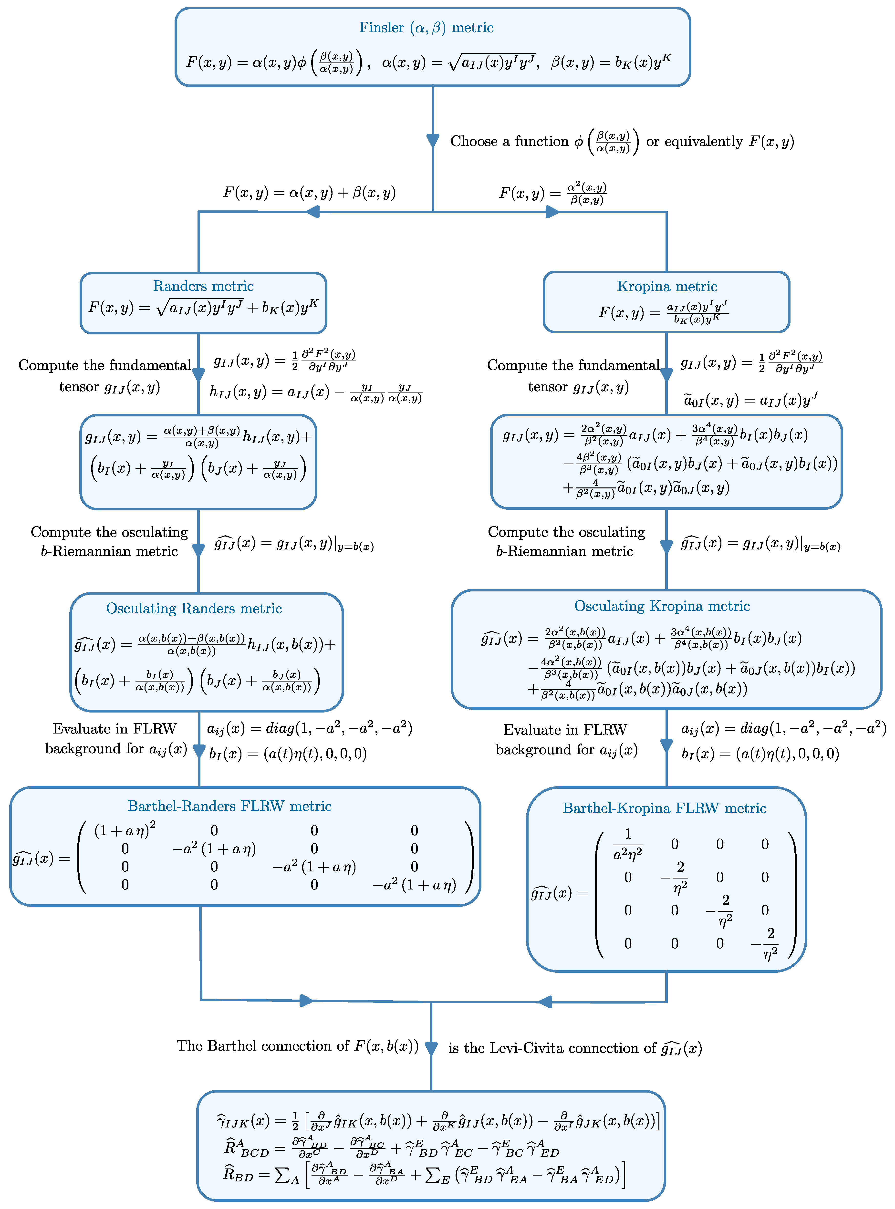
The steps necessary to construct a specific Barthel-Kropina type cosmological model, and the underlying gravitational theory, are presented algorithmically in the form of a flowchart in Figure 1.

Although specific examples are restricted to the cases of Barthel-Randers and Barthel-Kropina geometries, the formalism can be easily extended to any other choices of the Finslerian function $F=\alpha \varphi \left(s\right)$, and the implementation of the geometrical model into a gravitational theoretical framework can be done easily. In all these cases some extensions of standard general relativity can be obtained, leading to gravitational field equations that contain extra Finslerian terms, which in a cosmological context can be interpreted as describing an effective geometric dark energy, generated by the nonlocal geometric structure of the spacetime, with the metric tensor nonlocalized due to the presence of the vector y, representing an internal degree of freedom.

There are a large number of $(\alpha ,\beta )$ metrics, whose physical and gravitational properties is worth investigating, and which could offer new and important insights into the gravitational and cosmological phenomena. The flowchart of the algorithmic approach presented in Figure 1 may simplify and clarify the necessary steps taken for the investigation of these classes of theories.

Figure 1. Flowchart of the algorithmic approach for the construction of the $(\alpha ,\beta )$ gravitational models with the Barthel connection.

Figure 1. Flowchart of the algorithmic approach for the construction of the $(\alpha ,\beta )$ gravitational models with the Barthel connection.

3.3. Barthel-Randers Cosmology

For the case of the Randers geometry we have $F=\alpha +\beta$. By using the above assumptions it turns out that the generalized Friedmann equations in this geometry take the form [113]

$$3H^2=8\pi G{\varphi }^2\rho -{\displaystyle \frac{3}{4}}{\displaystyle \frac{{\dot{\varphi }}^2}{{\varphi }^2}}-3H{\displaystyle \frac{\dot{\varphi }}{\varphi }},$$

(60)

and

$$2\dot{H}+3H^2=-{\displaystyle \frac{8\pi G}{c^2}}{\varphi }^{2}p-{\displaystyle \frac{\ddot{\varphi }}{\varphi }}+{\displaystyle \frac{5}{4}}{\displaystyle \frac{{\dot{\varphi }}^2}{{\varphi }^2}}-H{\displaystyle \frac{\dot{\varphi }}{\varphi }},$$

(61)

respectively, where we have denoted

$$\varphi \left(x^0\right)=1+a\left(x^0\right)\eta \left(x^0\right).$$

(62)

Eqs. (60) and (61) give the dynamical evolution of H as

$$\dot{H}=-4\pi G{\varphi }^2\left(\rho +{\displaystyle \frac{p}{c^2}}\right)-{\displaystyle \frac{\ddot{\varphi }}{2\varphi }}+{\displaystyle \frac{{\dot{\varphi }}^2}{{\varphi }^2}}+H{\displaystyle \frac{\dot{\varphi }}{\varphi }}.$$

(63)

Eq. (60) can be rewritten as

$$3{\left(H+{\displaystyle \frac{\dot{\varphi }}{2\varphi }}\right)}^2=8\pi G{\varphi }^2\rho .$$

(64)

By introducing the new Hubble function defined as

$$\tilde{H}=H+{\displaystyle \frac{\dot{\varphi }}{2\varphi }},$$

(65)

we obtain the final form of the generalized Friedmann equations in the Barthel-Randers cosmology as

$$3{\tilde{H}}^2=8\pi G{\varphi }^2\rho ,$$

(66)

and

$$2\dot{\tilde{H}}+3{\tilde{H}}^2=-{\displaystyle \frac{8\pi G}{c^2}}{\varphi }^{2}p+{\displaystyle \frac{{\dot{\varphi }}^2}{{\varphi }^2}}+2H{\displaystyle \frac{\dot{\varphi }}{\varphi }},$$

(67)

respectively.

The Energy Conservation Equation

The energy conservation equation of the matter in the present model of the Barthel-Randers cosmology can be obtained by assuming that similarly to the standard Riemannian general relativistic case, the covariant divergence of the energy-momentum tensor vanishes, ${\widehat{\nabla }}_{\mu }{T}^{\mu \nu }=0$, with the covariant derivative calculated with the help of the Barthel-Randers connection ${{\widehat{\gamma }}^{\mu }}_{\nu \alpha }$. Hence, the conservation equation in Barthel-Randers cosmology can be written as [113]

$$\dot{\rho }+3\left(H+{\displaystyle \frac{\dot{\varphi }}{2\varphi }}\right)\left(\rho +{\displaystyle \frac{p}{c^2}}\right)=0,$$

(68)

or, in an alternative form, as

$${\displaystyle \frac{d}{dt}}\left(\rho a^3\right)+{\displaystyle \frac{p}{c^2}}{\displaystyle \frac{d}{dt}}{a}^3+{\displaystyle \frac{3}{2}}{a}^3\left(\rho +{\displaystyle \frac{p}{c^2}}\right)=0.$$

(69)

The conservation equation is not independent, and can be also derived directly with the use of the Friedman equations. By taking the time derivative of Eq. (60), and after substituting $\dot{H}$ from Eq. (61), we find

$$\begin{array}{cc}\hfill & 8\pi G{\varphi }^2\left(\dot{\rho }+{\displaystyle \frac{3Hp}{c^2}}\right)-{\displaystyle \frac{3}{8{\varphi }^3}}({\dot{\varphi }}^3-2H\varphi {\dot{\varphi }}^2-20H^2{\varphi }^2{\dot{\varphi }}^2)\hfill \\ & +4\pi G\varphi \dot{\varphi }(3p+4\rho )+9H^3=0.\hfill \end{array}$$

(70)

By substituting the expression of $H^2$ from the Friedman equation (60), we recover Eq. (70).

3.4. Barthel-Kropina Cosmology

In the Kropina geometry the Finslerian metric function is given by $F={\alpha }^2/\beta$. The generalized Friedmann equations, can be obtained directly from the Einstein equations, and are given by [114]

$${\displaystyle \frac{3{\left({\eta }^{\prime }\right)}^2}{{\eta }^2}}={\displaystyle \frac{8\pi G}{c^2}}{\displaystyle \frac{1}{a^2{\eta }^2}}\rho ,$$

(71)

and

$$2{\displaystyle \frac{{\eta }^{\prime \prime }}{\eta }}+2\mathcal{H}{\displaystyle \frac{{\eta }^{\prime }}{\eta }}-3{\displaystyle \frac{{\left({\eta }^{\prime }\right)}^2}{{\eta }^2}}={\displaystyle \frac{8\pi G}{c^4}}{\displaystyle \frac{p}{a^2{\eta }^2}},$$

(72)

respectively, where by $\mathcal{H}$ we have denoted the generalized Hubble function of the Barthel-Kropina cosmology, defined according to $\mathcal{H}=\left(1/a\left(x^0\right)\right)\left(da\left(x^0\right)/d{x}^0\right)$.

In the above equations, and in the following, a prime denotes the derivative with respect to $x^0$, a dot denotes the derivative with respect to the cosmological time t, and the standard Hubble function is given by $H=c\mathcal{H}$. After eliminating the term $-3{\left({\eta }^{\prime }\right)}^2$ with the help of Eq. (71), Eq. (72) becomes [114]

$$a\eta {\displaystyle \frac{d}{d{x}^0}}\left({\eta }^{\prime }a\right)={\displaystyle \frac{4\pi G}{c^4}}\left(\rho c^2+p\right).$$

(73)

In the Barthel-Kropina geometry the full system of the generalized Friedmann equations is represented by two ordinary differential equations with four unknowns $\left(a,\eta ,\rho ,p\right)$. By considering an equation of state for the baryonic matter, $p=p\left(\rho \right)$, the number of unknowns in the system of generalized Friedmann equations becomes three, and the system is still underdetermined. Therefore, to obtain solvable cosmological models, and to close the system, we must impose a supplementary independent relation on two of the model parameters.

Energy Balance Equation

One of the basic consequences of the standard Friedmann cosmology is the conservation of the matter energy-momentum tensor. But as one can easily observe from the Friedmann equations (71) and (72), this property does not hold anymore in the Barthel-Kropina cosmology. The matter non-conservation equation matter as well as the energy density balance equation can be obtained after the multiplication of Eq. (71) with $a^3$, and applying the time derivation operator $d/d{x}^0$ on the result. By using in the obtained relation the second generalized Friedmann equation, the energy nonconservation equation in the Barthel-Kropina cosmology is obtained as [114]

$$\begin{array}{c}\hfill {\displaystyle \frac{8\pi G}{c^4}}\left[{\displaystyle \frac{d}{d{x}^0}}\left(\rho c^2{a}^3\right)+p{\displaystyle \frac{d}{d{x}^0}}{a}^3\right]=6a^5\left[\mathcal{H}{\left({\eta }^{\prime }\right)}^2+\left({\eta }^{\prime }+\mathcal{H}\eta \right){\eta }^{\prime \prime }+{\mathcal{H}}^2\eta {\eta }^{\prime }\right].\end{array}$$

(74)

Eq. (74) can be written in a form similar to the standard general relativistic conservation equation as

$$\begin{array}{c}\hfill {\displaystyle \frac{4\pi G}{c^4}}\left[{\displaystyle \frac{d}{d{x}^0}}\left(\rho c^2{a}^3\right)+p{\displaystyle \frac{d}{d{x}^0}}{a}^3\right]=3a^5\left[{\displaystyle \frac{8\pi G}{2c^4}}\left({\displaystyle \frac{5}{3}}\rho c^2+p\right){\displaystyle \frac{\mathcal{H}}{a^2}}+{\eta }^{\prime }{\eta }^{\prime \prime }\right].\end{array}$$

(75)

The General Relativistic Limit

An interesting and important property of the generalized Friedmann equations of the Barthel-Kropina cosmological model, given by Eqs. (71) and (72), respectively, is that they admit a general relativistic limit, in which they take the form of the standard Friedmann equations of general relativity. The general relativistic limit is given by [114]

$$\eta \to \pm {\displaystyle \frac{1}{a}},\beta \to (1,0,0,0).$$

(76)

Then from Eqs. (71) and (72) we immediately reobtain the Friedmann equations of standard general relativity

$${\displaystyle \frac{3{\left(a^{\prime }\right)}^2}{a^2}}={\displaystyle \frac{8\pi G}{c^2}}\rho ,2{\displaystyle \frac{a^{\prime \prime }}{a}}+{\displaystyle \frac{{\left(a^{\prime }\right)}^2}{a^2}}=-{\displaystyle \frac{8\pi G}{c^4}}p.$$

(77)

From Eqs. (77) it follows that the energy density $\rho$ is conserved, with the conservation equation given by $\dot{\rho }+3H\left(\rho +p/c^2\right)=0$.

3.5. Conformal Barthel-Kropina Cosmology

Let’s consider that an $(\alpha ,\beta )$-metric with $F=F(\alpha ,\beta )$ is given. The conformal transformation of the metric is defined as [116]

$$\tilde{F}(x,y):=e^{\sigma \left(x\right)}F(x,y)=\tilde{F}\left(\tilde{\alpha },\tilde{\beta }\right).$$

(78)

The metric (78) is again an $\left(\tilde{\alpha },\tilde{\beta }\right)$ metric, with

$$\tilde{\alpha }=e^{\sigma \left(x\right)}\alpha ,\tilde{\beta }=e^{\sigma \left(x\right)}\beta .$$

(79)

The fundamental tensor of $\tilde{F}$ is calculated with the help of the Hessian [116]

$${\tilde{g}}_{IJ}:={\displaystyle \frac{1}{2}}{\displaystyle \frac{{\partial }^2{\tilde{F}}^2}{\partial y^I\partial y^J}}.$$

(80)

The conformal transformation of the Kropina metric is obtained as

$$\tilde{F}:=e^{\sigma \left(x\right)}{\displaystyle \frac{{\alpha }^2}{\beta }}={\displaystyle \frac{{\tilde{\alpha }}^2}{\tilde{\beta }}},$$

where $\tilde{\alpha }=e^{\sigma \left(x\right)}\alpha$, $\tilde{\beta }=e^{\sigma \left(x\right)}\beta$. The osculating Riemannian metric is obtained as

$${\widehat{\tilde{g}}}_{IJ}\left(x\right)=e^{2\sigma \left(x\right)}{\widehat{g}}_{IJ}\left(x\right),$$

(81)

where ${\widehat{g}}_{IJ}\left(x\right)$ is given by

$$\begin{array}{ccc}\hfill {\widehat{g}}_{IJ}(x,b\left(x\right))& =& {\displaystyle \frac{2{\alpha }^2}{{\beta }^2}}{a}_{IJ}\left(x\right)+{\displaystyle \frac{3{\alpha }^4}{{\beta }^4}}{b}_I{b}_J-{\displaystyle \frac{4{\alpha }^2}{{\beta }^3}}(b_I{b}_J+b_J{b}_I)+{\displaystyle \frac{4}{{\beta }^2}}{b}_I{b}_J,\hfill \end{array}$$

(82)

where $b_I:=a_{IJ}{b}^J={\tilde{a}}_{0I}(x,b\left(x\right))$ (see flowchart 1). For cosmological applications we choose the conformal factor as $\sigma \left(x\right)=\varphi \left(x^0\right)$. Hence in the study of the dynamical evolution of the Universe we will restrict our investigations to conformal transformations of the Kropina metric that depend only on time.

The Generalized Friedmann Equations

In the conformal Barthel-Kropina geometry the generalized Friedmann equations take the form [116]

$${\displaystyle \frac{3{\left({\eta }^{\prime }\right)}^2}{{\eta }^2}}={\displaystyle \frac{8\pi G}{c^2}}{\displaystyle \frac{1}{a^2{\eta }^2}}\tilde{\rho }+3{\left({\varphi }^{\prime }\right)}^2-6{\displaystyle \frac{{\eta }^{\prime }}{\eta }}{\varphi }^{\prime },$$

(83)

and

$$\begin{array}{ccc}\hfill & & {\displaystyle \frac{2}{{\eta }^2}}[-3{\left({\eta }^{\prime }\right)}^2+2\eta {\eta }^{\prime }\mathcal{H}+2\eta {\eta }^{\prime \prime }]={\displaystyle \frac{16\pi G}{c^4}}{\displaystyle \frac{1}{a^2{\eta }^2}}\tilde{p}\hfill \\ & & -4\left[{\varphi }^{\prime \prime }+{\displaystyle \frac{1}{2}}{\left({\varphi }^{\prime }\right)}^2\right]+\left({\displaystyle \frac{{\eta }^{\prime }}{\eta }}-\mathcal{H}\right){\varphi }^{\prime },\hfill \end{array}$$

(84)

respectively. We eliminate now the term $-3{\left({\eta }^{\prime }\right)}^2/{\eta }^2$ between Eqs. (83) and (84), and thus we find the relation

$$\begin{array}{ccc}\hfill 2{\displaystyle \frac{1}{a\eta }}{\displaystyle \frac{d}{d{x}^0}}\left(a{\eta }^{\prime }\right)& =& {\displaystyle \frac{4\pi G}{c^4}}{\displaystyle \frac{1}{a^2{\eta }^2}}\left(\tilde{\rho }{c}^2+\tilde{p}\right)-\left({\varphi }^{\prime \prime }-{\left({\varphi }^{\prime }\right)}^2\right)-{\displaystyle \frac{11}{4}}{\displaystyle \frac{{\eta }^{\prime }}{\eta }}{\varphi }^{\prime }-{\displaystyle \frac{1}{4}}{\varphi }^{\prime }\mathcal{H}.\hfill \end{array}$$

(85)

The general relativistic limit of the system (83)-(84) is obtained by taking $\eta \to 1/a$, and $\left(b_I\left(x\right)\right)=(1,0,0,0)$, respectively. Consequently, $\beta =y^0$. Thus, in this limit, the generalized Friedmann cosmological evolution equations of the conformal Barthel-Kropina model become [116]

$$3{\mathcal{H}}^2={\displaystyle \frac{8\pi G}{c^4}}\tilde{\rho }{c}^2+3{\left({\varphi }^{\prime }\right)}^2+6\mathcal{H}{\varphi }^{\prime },$$

(86)

and

$$2{\mathcal{H}}^{\prime }+3{\mathcal{H}}^2=-{\displaystyle \frac{8\pi G}{c^4}}\tilde{p}+2\left[{\varphi }^{\prime \prime }+{\displaystyle \frac{1}{2}}{\left({\varphi }^{\prime }\right)}^2\right]+\mathcal{H}{\varphi }^{\prime },$$

(87)

respectively. For $\varphi =0$ we fully recover the standard Friedmann equations of general relativity.

3.6. Thermodynamic Interpretation of the $(\alpha ,\beta )$ Cosmologies

It is a general property of several Finslerian type cosmological models that the matter energy-momentum is not conserved. For example, Eq. (68) illustrate this situation for the case of the Barthel-Randers cosmological models. Hence, contrary to the general relativistic case, in the Barthel-Randers type cosmological model, as well as in the Barthel-Kropina and conformally transformed Barthel-Kropina cosmologies, the baryonic matter content of the Universe is not conserved anymore. This intriguing property of the models raises the problem of the physical interpretation of the nonconservation of the matter energy-momentum tensor, and the problem of the cosmological significance of this effect.

A possible physical understanding of the energy-momentum nonconservation can be obtained by interpreting this effect by using the thermodynamics of irreversible processes, and assuming that it describes particle creation and annihilation in a cosmological environment. In the following we briefly introduce first the foundations of the thermodynamic of irreversible processes, and then we illustrate the general formalism by considering the specific case of the Barthel-Randers type cosmological model. The nonconservation of the energy-momentum tensor is a specific feature of several modified gravity theories, and specifically in approaches to gravity involving the presence of geometry-matter coupling [137]. Example of such theories are the $f\left(R,L_m\right)$[138] and the $f(R,T)$ [139] theories.

The non-conservation of the matter energy-momentum tensor, as shown, for example, for the Barthel-Randers case by Eq. (68), can thus be interpreted as showing that due to the existence of the Finslerian geometric effects, during the cosmological evolution matter creation processes may take place during the cosmological evolution. This indicates the possibility of creating matter from geometry. Quantum field theories in curved space-time also predict the same particle creation effect, as initially proposed and investigated in [140,141,142,143,144,145]. In quantum field theory particle creation is due to the time variation of the gravitational field. In an anisotropic Bianchi type I metric quantum particle creation was considered in [142], and for a quantum scalar field with a non-zero mass the renormalized expression of the energy-momentum tensor was determined. Hence, the osculating Finsler-Barthel type gravity theories, in which the creation of matter is also allowed by the general formalism, could also be interpreted as providing an effective, semiclassical description of the quantum effects in the gravitational field. It is important to note, however, that the nature of the particles is not necessarily known, unless quantum theoretical effects are taken into account.

3.6.1. Irreversible Thermodynamics and Matter Creation

Eq. (68), obtained within the framework of the Barthel-Randers cosmology, shows that the covariant divergence of the energy-momentum tensor, which is a function of the equilibrium quantities of the thermodynamic system represented by the baryonic matter, is different from zero. Similar effects do appear for the case of other thermodynamical quantities, like, for example, the particle and entropy fluxes. Hence, in the presence of matter creation all the balance equilibrium equations must be modified to account for this effect [146,147,148]. We will present first the general formalism of irreversible thermodynamics in the presence of matter creation, by adopting a cosmological perspective. We will consider all the results in the Riemann space, with metric $a_{AB}\left(x\right)$. Moreover, we interpret the Finslerian effects as generating a set of specific physical events in the background Riemann geometry. Hence, in the following all the physical and geometrical quantities will be expressed with the help of the FLRW metric (56). Consequently, all considered physical and geometrical quantities are functions of the cosmological time t only.

Particle Balance Equations

To describe particle dynamics we introduce the particle number density n, and the four-velocity $u^I$ of matter. From these quantities we construct the particle flux $N^I\equiv n{u}^I$. All these physical parameters are defined in Riemannian geometry. The particle balance equation in the presence of matter creation is given by

$${\nabla }_I{N}^I=\dot{n}+3Hn=n\Gamma ,$$

(88)

where ${\nabla }_I$ is the covariant derivative defined in the Riemann space with the help of the Levi-Civita connection associated to the FLRW metric (56), while $\Gamma$ denotes the matter creation rate. For $\Gamma \ll 3H$, the source term in the particle balance equation is negligible, and we reobtain the standard particle conservation law of general relativity.

The Entropy Flux

We introduce now the entropy density $\tilde{s}$, and the entropy per particle $\sigma =\tilde{s}/n$. From these quantities we construct the entropy flux vector defined as $S^I\equiv \tilde{s}{u}^I=n\sigma u^I$. The divergence of the entropy flux gives the relation

$${\nabla }_I{S}^I=n\dot{\sigma }+n\sigma \Gamma \ge 0,$$

(89)

where the positivity condition is a direct consequence of the second law of thermodynamics. The case $\sigma =\mathrm{constant}$ gives the relation

$${\nabla }_I{S}^I=n\sigma \Gamma =\tilde{s}\Gamma \ge 0.$$

(90)

Eq. (90) shows that if the entropy per particle can be taken as a constant, then the variation of the entropy is only due to the matter generated via the transfer of the energy of the gravitational field to matter. Since $\tilde{s}>0$, the particle production rate $\Gamma$ must satisfy the basic thermodynamic condition $\Gamma \ge 0$. From a physical point of view this condition can be interpreted as permitting the creation of matter from the gravitational field, but suppressing the opposit process.

The Creation Pressure

If particle creation takes place, the matter energy-momentum tensor must also be modified to take into account the presence of the irreversible processes and the second law of thermodynamics. Generally, in the thermodynamical description of open systems, the energy-momentum tensor can be represented as [149]

$$T^{IJ}=T_{\mathrm{eq}}^{IJ}+\Delta T^{IJ},$$

(91)

where $T_{\mathrm{eq}}^{IJ}$ is the equilibrium thermodynamic component [149], and $\Delta T^{IJ}$ describes the supplementary terms induced by particle creation. For a homogeneous and isotropic space-time geometry, $\Delta T^{IJ}$, giving the particle creation contribution to $T^{IJ}$, can be generally represented in the form

$$\Delta T_0^0=0,\Delta T_I^J=-P_c{\delta }_I^J,$$

(92)

where $P_c$ denotes the creation pressure, an effective thermodynamic quantity, which in a macroscopic physical system describes phenomenologically particle creation. Moreover, in a fully covariant representation the tensor $\Delta T^{IJ}$ is given by [149]

$$\Delta T^{IJ}=-P_c{h}^{IJ}=-P_c\left(a^{IJ}-u^I{u}^J\right),$$

(93)

where $h^{IJ}=a^{IJ}-u^I{u}^J$ is the projection operator defined in the FLRW geometry. Thus, we obtain straightforwardly the relation $u_I{\nabla }_J\Delta T^{IJ}=3H{P}_c$.

In the presence of particle production by the gravitational field, from the scalar component of the energy balance equation $u_I{\nabla }_J{T}^{IJ}=0$, obtained from Eq. (91), we obtain the time variation of the energy density $\rho$ of the cosmological fluid as

$$\dot{\rho }+3H\left[\rho +{\displaystyle \frac{1}{c^2}}\left(p+P_c\right)\right]=0.$$

(94)

The thermodynamic quantities describing baryonic matter must also satisfy the Gibbs law [147]

$$nTd\left({\displaystyle \frac{\tilde{s}}{n}}\right)=nTd\sigma =d\rho -{\displaystyle \frac{\rho +p/c^2}{n}}dn,$$

(95)

where by T is the temperature of the cosmological matter.

3.6.2. Application: Particle Creation in Barthel-Randers Cosmology

As an example of the application of the irreversible thermodynamic of open systems we consider now the interpretation of the Barthel-Randers cosmology as a cosmological theory also describing particle creation during the evolution of the Universe.

Creation Pressure in Barthel-Randers Cosmology

After some simple algebraic transformations, the particle energy balance equation (68) of the Barthel-Randers cosmology can be rewritten as

$$\dot{\rho }+3H\left[\left(\rho +{\displaystyle \frac{p}{c^2}}\right)\left(1+{\displaystyle \frac{\dot{\varphi }}{2H\varphi }}\right)\right]=0.$$

(96)

By comparing Eqs. (94) and (96) we find the expression of the Barthel-Randers creation pressure as

$$P_c={\displaystyle \frac{\dot{\varphi }}{2H\varphi }}\left(\rho c^2+p\right)={\displaystyle \frac{c^2\rho \dot{\varphi }}{2H\varphi }}\left(1+\omega \right),$$

(97)

where $\omega =p/\rho c^2$. The energy density balance Eq. (68) can now be derived equivalently from the divergence of the total energy momentum tensor $T^{IJ}$, given by

$$T^{IJ}=\left(\rho c^2+p+P_c\right)u^I{u}^J-\left(p+P_c\right)a^{IJ},$$

(98)

where all the mathematical operations must be performed in the Riemann space with the FLRW metric (56).

The Particle Creation Rate

By assuming adiabatic particle production, which requires that $\dot{\sigma }=0$, the Gibbs relation (95) gives

$$\dot{\rho }=\left(\rho +{\displaystyle \frac{p}{c^2}}\right){\displaystyle \frac{\dot{n}}{n}}=\left(\rho +{\displaystyle \frac{p}{c^2}}\right)\left(\Gamma -3H\right).$$

(99)

By combining this relation with the energy balance equation (96) we obtain the particle creation rate as a function of the creation pressure, the Hubble function and the equilibrium thermodynamic quantities as

$$\Gamma ={\displaystyle \frac{-3H{P}_c}{\rho c^2+p}}.$$

(100)

By using Eq. (97) we find for the Barthel-Randers cosmological particle creation rate the expression

$$\begin{array}{c}\hfill \Gamma =-{\displaystyle \frac{3}{2}}{\displaystyle \frac{\dot{\varphi }}{\varphi }}=-{\displaystyle \frac{3}{2}}{\displaystyle \frac{d}{dt}}ln\varphi =-{\displaystyle \frac{3}{2}}{\displaystyle \frac{\dot{a}\eta +a\dot{\eta }}{1+a\eta }}.\end{array}$$

(101)

If $1+a\eta >0$, the condition $\Gamma \ge 0$, which is equivalent with the existence of particle creation, leads to the constraint

$$\dot{\varphi }=\dot{a}\eta +a\dot{\eta }=a\left(\dot{\eta }+H\eta \right)\le 0,$$

(102)

on the scale factor a, and the temporal component of the one-form $\eta$. The condition does not depend explicitly on the equation of state of the baryonic matter, but an indirect dependence via the Hubble function does exist. The condition $\dot{\varphi }<0$ implies the existence of a negative creation pressure, as it follows from Eq. (97). Therefore particle production is thermodynamically allowed only if the creation pressure is negative, $P_c<0$.

The Barthel-Randers particle balance equation can thus be reformulated to take the form

$$\dot{n}+3Hn=-{\displaystyle \frac{3}{2}}n{\displaystyle \frac{\dot{\varphi }}{\varphi }}=\Gamma n,$$

(103)

and it can be integrated to give for the particle number density the expression

$$n={\displaystyle \frac{n_0}{{\varphi }^{3/2}{a}^3}},$$

(104)

where $n_0$ is a constant of integration.

For an Universe consisting of pressureless dust with $p=0$, the creation pressure is given by

$$P_c={\displaystyle \frac{\dot{\varphi }}{2H\varphi }}\rho c^2={\displaystyle \frac{\rho c^2}{2H}}{\displaystyle \frac{d}{dt}}ln\varphi ,$$

(105)

and it depends linearly on the baryonic matter density.

The divergence of the entropy flux vector $S^I$ takes the form

$${\nabla }_I{S}^I={\displaystyle \frac{-3n\sigma H{P}_c}{\rho c^2+p}}=-{\displaystyle \frac{3}{2}}n\sigma {\displaystyle \frac{\dot{\varphi }}{\varphi }}=n\sigma \Gamma .$$

(106)

The Matter Temperature

The temperature T of the baryonic matter represents an important characteristic of physical systems. To obtain the temperature evolution in the presence of particle creation, we consider the general thermodynamic case in which the density and the pressure are functions of the particle number density, and of the temperature. Hence $\rho$ and p can be generally represented in parametric form $\rho =\rho (n,T)$ and $p=p(n,T)$, respectively. Then we obtain

$$\dot{\rho }={\left({\displaystyle \frac{\partial \rho }{\partial n}}\right)}_T\dot{n}+{\left({\displaystyle \frac{\partial \rho }{\partial T}}\right)}_n\dot{T}.$$

(107)

By using the energy and particle balance equations we find first the relation

$$-3H\left(\rho c^2+p+P_c\right)={\left({\displaystyle \frac{\partial \rho }{\partial n}}\right)}_{T}n\left(\Gamma -3H\right)+{\left({\displaystyle \frac{\partial \rho }{\partial T}}\right)}_n\dot{T}.$$

(108)

As a second step we use of the thermodynamic relation [149]

$$T{\left({\displaystyle \frac{\partial p}{\partial T}}\right)}_n=\rho c^2+p-n{\left({\displaystyle \frac{\partial \rho }{\partial n}}\right)}_T,$$

(109)

which together with Eq. (108) gives the temperature evolution of the matter in the Barthel-Randers cosmology in the presence of particle production as

$${\displaystyle \frac{\dot{T}}{T}}={\displaystyle \frac{1}{c^2}}{\left({\displaystyle \frac{\partial p}{\partial \rho }}\right)}_n{\displaystyle \frac{\dot{n}}{n}}=\omega {\displaystyle \frac{\dot{n}}{n}}.$$

(110)

From the particle balance equation we obtain the ratio $\dot{n}/n$ as

$${\displaystyle \frac{\dot{n}}{n}}=-3\left({\displaystyle \frac{\dot{\varphi }}{\varphi }}+{\displaystyle \frac{\dot{a}}{a}}\right).$$

(111)

By assuming that $\dot{\varphi }<0$, we obtain for the temperature evolution of the particles in the Barthel-Randers Universe the relation

$$T=T_0{\displaystyle \frac{{\varphi }^{3\omega /2}}{a^3}}.$$

(112)

Generally, $\omega$ is an arbitrary scale factor dependent parameter $\omega =\omega \left(a\right)$[150]. In a thermodynamically consistent cosmological model all geometrical and physical quantities must be well-defined and regular for all $\omega \left(a\right)$.

3.6.3. Creation of Exotic Matter

In our discussion of the thermodynamic of open systems, as presented in the previous Section, we have assumed that matter is created in the form of baryonic matter, satisfying the energy condition $\rho c^2+p\ge 0$, and the restriction on the parameter of the matter equation of state $\omega \ge 0$. But we cannot a priori exclude the possibility case in which an exotic fluid with $\omega <0$ is created during the cosmological evolution of the Barthel-Randers Universe. The open system thermodynamic approach to particle creation considered previously is also applicable if $\omega <0$. For this case the creation pressure becomes negative for $\dot{\varphi }>0$, with the particle creation rate $\Gamma$ becoming positive. Therefore, matter creation processes generating exotic particles can also be included in the Barthel-Randers cosmological model.

A particular and important case is represented by an exotic fluid satisfying the equation of state ${\rho }_{\left(ex\right)}{c}^2+p_{\left(ex\right)}=0$, with $\omega =-1$, which is equivalent to the presence of a cosmological constant. Then from Eq. (94) we obtain

$${\dot{\rho }}_{\left(ex\right)}=-3H{P}_c.$$

(113)

If the exotic particle creation process is adiabatic, with $\dot{\sigma }=0$, from the Gibbs relation we find

$${\dot{\rho }}_{\left(ex\right)}=\left({\rho }_{\left(ex\right)}{c}^2+p_{\left(ex\right)}\right){\displaystyle \frac{{\dot{n}}_{\left(ex\right)}}{n_{\left(ex\right)}}}=0.$$

(114)

The above two equations give independently

$${\dot{\rho }}_{\left(ex\right)}=P_c=0,$$

(115)

which describe an Universe with constant exotic matter density, and vanishing creation pressure. On the other hand if $\omega =-2$, and ${\rho }_{\left(ex\right)}>0$, then $P_c=-\left(c^2\dot{\varphi }/2H\varphi \right){\rho }_{\left(ex\right)}$, $\Gamma =(3/2)\dot{\varphi }/\varphi$, and matter production can take place if the conditions $\dot{\varphi }>0$ and $\varphi >0$ are satisfied.

Thus in a Barthel-Randers Universe the creation of exotic matter or possibly of scalar fields is allowed in a way consistent with the laws of thermodynamics. The creation processes take place in the Riemannian geometry characterized by the FLRW metric.

4. Cosmological Implications of Barthel Randers and Barthel-Kropina Models

In this Section, we investigate the cosmological implications of the Barthel-Randers and Barthel-Kropina models by exploring three distinct variants of the Barthel-Randers framework alongside the Barthel-Kropina cosmological model. To constrain the free parameters of these models, we employ a combination of observational datasets, including Type Ia supernovae, baryon acoustic oscillations, and Hubble parameter measurements. By extracting the posterior distributions of the model parameters through Bayesian inference, we are able to assess the observational viability of the Barthel-Randers and Barthel-Kropina models. This comparison with the standard $\Lambda$CDM cosmology enables us to explore possible deviations from the conventional expansion history and to evaluate whether these geometrically extended models offer a competitive or improved description of the Universe’s evolution.

4.1. Specific Cosmological Models

In this subsection, we present the normalized Hubble functions associated with both the Barthel-Randers [113] and Barthel-Kropina [114] cosmological models. Our starting point is the family of cosmological scenarios proposed in [113], where three distinct variants of the Barthel-Randers model were introduced. Each of these variants is characterized by a specific choice of the function $\phi \left(z\right)$. The normalized Hubble function for all three models can be expressed in a unified form as

$$h\left(z\right)={\displaystyle \frac{2\phi \left(z\right)\sqrt{{(1+z)}^3\sqrt{\phi \left(z\right)}{\Omega }_{m0}+\phi {\left(z\right)}^2{\Omega }_{\Lambda 0}+{(1+z)}^4{\Omega }_{r0}}}{(1+z)\frac{d\phi \left(z\right)}{dz}-2\phi \left(z\right)}},$$

(116)

where z is the redshift, ${\Omega }_{m0}$, ${\Omega }_{\Lambda 0}$, and ${\Omega }_{r0}$ are the present-day matter, dark energy, and radiation density parameters, respectively. The dark energy density parameter ${\Omega }_{\Lambda 0}$ is obtained through the constraint

$${\Omega }_{\Lambda 0}={\left(1-{\displaystyle \frac{1}{2}}{\phi }^{\prime }\left(0\right)\right)}^2-{\Omega }_{m0}-{\Omega }_{r0},$$

(117)

where ${\phi }^{\prime }\left(0\right)$ is the derivative of the function $\phi \left(z\right)$ evaluated at $z=0$. The form of $\phi \left(z\right)$ determines the behavior of each specific model and encodes the influence of the underlying Finslerian geometry. In the following, we present the explicit forms of $\phi \left(z\right)$ corresponding to each of the three models proposed in [113]:

• Linear model: $\phi \left(z\right)=1+\beta z$,
• Logarithmic model: $\phi \left(z\right)=1+ln(1+\beta z)$,
• Exponential model: $\phi \left(z\right)=e^{2\beta z}$.

We can obtain the corresponding normalized Hubble function by plugging the corresponding form of $\phi \left(z\right)$ into Eq. (116).

In the case of the Barthel-Kropina geometry, we adopt the model proposed by [114]. The corresponding normalized Hubble function is expressed as a system of differential equations in the redshift representation as follows

$${\displaystyle \frac{df\left(z\right)}{dz}}=-{\displaystyle \frac{u\left(z\right)}{(1+z)h\left(z\right)}},$$

(118)

$$\begin{array}{cc}\hfill {\displaystyle \frac{du\left(z\right)}{dz}}={\displaystyle \frac{1+f\left(z\right)}{2(1+z)h\left(z\right)}}[& 2h\left(z\right)\left({\displaystyle \frac{2}{1+f\left(z\right)}}-3\omega (1+f\left(z\right))\right)u\left(z\right)\hfill \\ \hfill & +3\left(\omega -{\displaystyle \frac{1}{{(1+f\left(z\right))}^2}}\right)u{\left(z\right)}^2+3\omega f\left(z\right)(2+f\left(z\right))h{\left(z\right)}^2],\hfill \end{array}$$

(119)

$${\displaystyle \frac{dh\left(z\right)}{dz}}={\displaystyle \frac{1}{2(1+z)h\left(z\right)}}\left[3h{\left(z\right)}^2-{\displaystyle \frac{4h\left(z\right)u\left(z\right)}{1+f\left(z\right)}}+{\displaystyle \frac{3u{\left(z\right)}^2}{{(1+f\left(z\right))}^2}}+{\displaystyle \frac{2(1+z)h\left(z\right)}{1+f\left(z\right)}}{\displaystyle \frac{du\left(z\right)}{dz}}\right].$$

(120)

The system of equations has to be solved with initial conditions $f\left(0\right)=f_0$, $u\left(0\right)=u_0$, and $h\left(0\right)=1$.

4.2. Methodology and Datasets

In this subsection, we provide a detailed explanation of the methodology used to estimate the posterior distributions of the model parameters, employing the Markov Chain Monte Carlo (MCMC) approach. This approach allows us to constrain model parameters by analyzing various observational datasets. The MCMC technique efficiently samples from the likelihood function while incorporating prior information, leading to a robust estimation of the posterior probability distribution [151]. It is important to note, that once the maximum posterior distribution is obtained, supposing the MCMC converged, one also has the maximum likelihood, which is a prior independent quantity, even if the posterior depends on the prior. Through this method, the model’s parameter space is thoroughly explored.

The MCMC algorithm works by taking samples from the posterior distribution, which is determined using Bayes’ theorem as

$$P\left(\theta \right|D)={\displaystyle \frac{L\left(D\right|\theta \left)P\right(\theta )}{P\left(D\right)}},$$

(121)

where $P\left(\theta \right|D)$ represents the probability of the parameters $\theta$ given the observational data D. The term $L\left(D\right|\theta )$ is the likelihood function, which measures how well the model fits the data. $P\left(\theta \right)$ is the prior distribution, incorporating any existing knowledge about the parameters, while $P\left(D\right)$ is the evidence, acting as a normalization factor [152].

One of the key advantages of the MCMC method is that it not only finds the most likely values for the parameters but also accounts for uncertainties in both the model and the observational data. We define the likelihood function in such a way that it compares the theoretical predictions of the Hubble parameter ($H\left(z\right)$), luminosity distance ($\mu \left(z\right)$), transverse distance ($D_H\left(z\right)$), comoving angular diameter distance ($D_M\left(z\right)$), and comoving volume distance ($D_V\left(z\right)$) with observational data, taking into account uncertainties through covariance matrices. The MCMC sampling is carried out using the emcee library [153], which has built in it an affine invariant ensemble sampler. This sampler is used to efficiently explore the parameter space. After running the MCMC chains with multiple walkers, we discard the initial burn-in steps to remove biases from the starting positions.

To visualize and analyze the posterior distributions, we utilize the GetDist package [154], which provides an extensive set of tools for generating 1D and 2D posterior distribution. In this work, we use three different observational datasets: Cosmic Chronometers, Type Ia supernovae, and Baryon Acoustic Oscillations.

Below, we provide a detailed description of each dataset and how the likelihood has been formed based on them.

• Cosmic Chronometers : In this study, we utilize the Hubble measurements extracted based on the differential age approach, as described in [155]. This technique leverages passively evolving massive galaxies, which formed at redshifts around $z\sim 2-3$, enabling a direct and model-independent determination of the Hubble parameter using the relationship $\Delta z/\Delta t$. This method significantly reduces the reliance on astrophysical assumptions [156,157].
  For our analysis, we use 15 Hubble measurements selected from the 31 Hubble measurements used in [158], which cover a redshift range from $0.179\le z\le 1.965$. We define the likelihood function for the CC dataset using the following expression: ${\mathcal{L}}_{\mathrm{CC}}=e^{{\displaystyle \frac{-1}{2}}(\Delta H^T\left(z\right){\mathbf{C}}^{-1}\Delta H\left(z\right))},$ with $\Delta \mathbf{H}\left(z\right)={\mathbf{H}}_{\mathrm{Model}}\left(\theta \right)-{\mathbf{H}}_{\mathrm{Obs}}$. Here, ${\mathbf{H}}_{\mathrm{Model}}\left(\theta \right)$ is the theoretical Hubble parameter, calculated at each redshift value $z_i$ using the model parameters $\theta$, while ${\mathbf{H}}_{\mathrm{obs}}$ represents the corresponding observed value of the Hubble parameter at the $i^{\mathrm{th}}$ redshift. Following [159], we use the full covariance matrix $\mathbf{C}$, which takes into account both statistical and systematic uncertainties in the observations. The inverse of this covariance matrix, ${\mathbf{C}}^{-1}$, is employed to incorporate these uncertainties into the likelihood function.
• Type Ia supernova : We also use the Pantheon⁺ dataset without the SHOES calibration, which consists of light curves from 1701 Type Ia Supernovae (SNe Ia) covering a redshift range of $0\le z\le 2.3$[160]. To analyze this data, we adopt the likelihood function described in [161], which incorporates the total covariance matrix, ${\mathbf{C}}_{\mathrm{total}}$, that includes both statistical (${\mathbf{C}}_{\mathrm{stat}}$) and systematic (${\mathbf{C}}_{\mathrm{sys}}$) uncertainties [162]. The likelihood function is given by: ${\mathcal{L}}_{\mathrm{SNe}\mathrm{Ia}}=e^{\left(-{\displaystyle \frac{1}{2}}{\mathbf{r}}^T{\mathbf{C}}_{\mathrm{total}}^{-1}\mathbf{r}\right)},$ where $\mathbf{r}$ represents the residual vector, defined as the difference between the observed and theoretical distance moduli: $r_i={\mu }_{\mathrm{obs}}\left(z_i\right)-{\mu }_{\mathrm{th}}(z_i,\theta )$, where $\theta$ Here, ${\mathbf{C}}_{\mathrm{total}}^{-1}$ is the inverse of the total covariance matrix. The model-predicted distance modulus is calculated as: ${\mu }_{\mathrm{model}}\left(z_i\right)=5{log}_{10}\left({\displaystyle \frac{d_L\left(z\right)}{\mathrm{Mpc}}}\right)+\mathcal{M}+25,$ where the luminosity distance $d_L\left(z\right)$ in a flat FLRW Universe is given by: $d_L\left(z\right)=c(1+z){\int }_0^z{\displaystyle \frac{d{z}^{\prime }}{H\left(z^{\prime }\right)}}.$ Here, c is the speed of light, and $H\left(z\right)$ is the Hubble parameter. This formulation highlights the degeneracy between the nuisance parameter $\mathcal{M}$ and the Hubble constant $H_0$.
• Baryon Acoustic Oscillation : In our analysis, we also incorporate the most recent Baryon Acoustic Oscillation (BAO) measurements from the Dark Energy Spectroscopic Instrument (DESI) Data Release 2 (DR2) [163]. The BAO scale is determined by the sound horizon at the drag epoch, $z_d\approx 1060$, given by: $r_d={\int }_{z_d}^{\infty }{\displaystyle \frac{c_s\left(z\right)}{H\left(z\right)}}dz,$ where $c_s\left(z\right)$ is a function of the baryon to photon densities ratio, and $H\left(z\right)$ is the Hubble parameter. In a flat $\Lambda$CDM model, $r_d=147.09\pm 0.26$ Mpc [63]. However, in this study, we treat $r_d$ as a free parameter, allowing late-time observations to constrain the corresponding model parameters [164,165,166,167,168]. For our analysis, we compute the following cosmological distance measures: the Hubble distance, $D_H\left(z\right)$, the comoving angular diameter distance, $D_M\left(z\right)$, and the volume-averaged distance, $D_V\left(z\right)$, given by: $D_H\left(z\right)={\displaystyle \frac{c}{H\left(z\right)}},D_M\left(z\right)=c{\int }_0^z{\displaystyle \frac{d{z}^{\prime }}{H\left(z^{\prime }\right)}},D_V\left(z\right)={\left[z{D}_M^2\left(z\right)D_H\left(z\right)\right]}^{1/3}.$ Here, c denotes the speed of light in vacuum. To constrain each model parameter, we analyze the following ratios: ${\displaystyle \frac{D_M\left(z\right)}{r_d}},{\displaystyle \frac{D_H\left(z\right)}{r_d}},{\displaystyle \frac{D_V\left(z\right)}{r_d}}.$ We also use the ratio $D_M\left(z\right)/D_H\left(z\right)$, which serves as an additional constraint independent of the sound horizon scale $r_d$. The likelihood function for the BAO data is given by: ${\mathcal{L}}_{\mathrm{BAO}}=exp\left(-{\displaystyle \frac{1}{2}}{\mathbf{r}}_Y^T·{\mathbf{C}}_{D_Y}^{-1}·{\mathbf{r}}_Y\right),$ where the residuals are defined as: ${\mathbf{r}}_Y=D_{Y,\mathrm{Model}}-D_{Y,\mathrm{Data}}$ with $Y={\displaystyle \frac{D_H}{r_d}},{\displaystyle \frac{D_M}{r_d}},{\displaystyle \frac{D_V}{r_d}},{\displaystyle \frac{D_M}{D_H}}.$ In our case, the statistical covariance matrix has been considered generally to be diagonal, with elements corresponding to the squared observational uncertainties and defined as : ${\mathbf{C}}_{D_Y}=\mathrm{diag}\left({\sigma }_{D_Y}^2\right),{\mathbf{C}}_{D_Y}^{-1}={\left(\mathrm{diag}\left({\sigma }_{D_Y}^2\right)\right)}^{-1}.$ The overall BAO likelihood function is then constructed as the product of the individual likelihoods: ${\mathcal{L}}_{\mathrm{BAO}}={\mathcal{L}}_{D_H/r_d}\times {\mathcal{L}}_{D_V/r_d}\times {\mathcal{L}}_{D_M/r_d}\times {\mathcal{L}}_{D_M/D_H}.$

The posterior distribution of model parameters is obtained by maximizing the likelihood function. The total likelihood function is given by

$${\mathcal{L}}_{\mathrm{tot}}={\mathcal{L}}_{\mathrm{CC}}\times {\mathcal{L}}_{\mathrm{SNe}\mathrm{Ia}}\times {\mathcal{L}}_{\mathrm{BAO}}.$$

(122)

First, we discuss how to extract the posterior distribution of the model parameters in the Barthel-Randers framework. To achieve these, we apply the standard approach outlined above. In these models, we treat the parameters $H_0$, ${\Omega }_{m0}$, $\beta$, $\mathcal{M}$, and $r_d$ as free parameters with the following priors: $H_0\left(\mathrm{km}{\mathrm{s}}^{-1}{\mathrm{Mpc}}^{-1}\right)\in [50,100],{\Omega }_{mo}\in [0,1],\mathcal{M}\in [-20,-18],r_d\left(\mathrm{Mpc}\right)\in [100,200]$, and $\beta$ as Gaussian distribution, as the model is sensitive to this parameter. The ${\Omega }_{r0}$ is extracted using the following relation: ${\Omega }_{r0}=\left(4.183699\times {10}^{-5}\right)h^{-2},$ where $h={\displaystyle \frac{H_0}{100}}$. In the case of the Linear and Logarithmic Models, ${\Omega }_{\Lambda 0}$ is extracted using the relation ${\Omega }_{\Lambda 0}=1-\beta +{\displaystyle \frac{{\beta }^2}{4}}-{\Omega }_{m0}-{\Omega }_{r0},$ while in the case of the Exponential Model, ${\Omega }_{\Lambda 0}$ is extracted using the relation: ${\Omega }_{\Lambda 0}=1-2\beta +{\beta }^2-{\Omega }_{m0}-{\Omega }_{r0}.$ This makes the explicit variation of ${\Omega }_{r0}$ and ${\Omega }_{\Lambda 0}$ redundant, as both are fully determined by the other parameters.

To constrain the Barthel-Kropina model, we begin by numerically solving the system of differential equations given in equations (118)–(120). These equations are integrated using the solve_ivp function from SciPy, employing the Radau method a fifth order implicit Runge–Kutta scheme particularly effective for handling the stiff differential equations. For numerical stability and accuracy over the redshift range $z\in [0,3]$, we set the relative and absolute tolerances to ${10}^{-3}$ and ${10}^{-6}$, respectively. After obtaining the numerical solutions, we use a MCMC approach to constrain the model parameters. For more information on how to handle these kind of Hubble like functions that appear within differential equations, please refer to [169]. In the case of the Barthel-Kropina model, we take the $H_0\left(\mathrm{km}{\mathrm{s}}^{-1}{\mathrm{Mpc}}^{-1}\right)\in [50,100],u_o\in [0.0,3.0],\mathcal{M}\in [-20,-18],r_d\left(\mathrm{Mpc}\right)\in [100,200],\mathrm{and}{f}_0$ as Gaussian distribution. It is important to note that in both cases, we work with the normalized Hubble function. The final Hubble parameter $H\left(z\right)$ can be obtained by multiplying the normalized function $h\left(z\right)$ with the Hubble constant $H_0$, i.e., $H\left(z\right)=H_0·h\left(z\right)$.

Figure 2. The constraints on the parameters of the Barthel-Randers and Barthel-Kropina cosmological models, showing both 1$\sigma$ and 2$\sigma$ confidence intervals. The contours show the correlations between these parameters, with marginalized probability distributions along the diagonal.

Figure 2. The constraints on the parameters of the Barthel-Randers and Barthel-Kropina cosmological models, showing both 1$\sigma$ and 2$\sigma$ confidence intervals. The contours show the correlations between these parameters, with marginalized probability distributions along the diagonal.

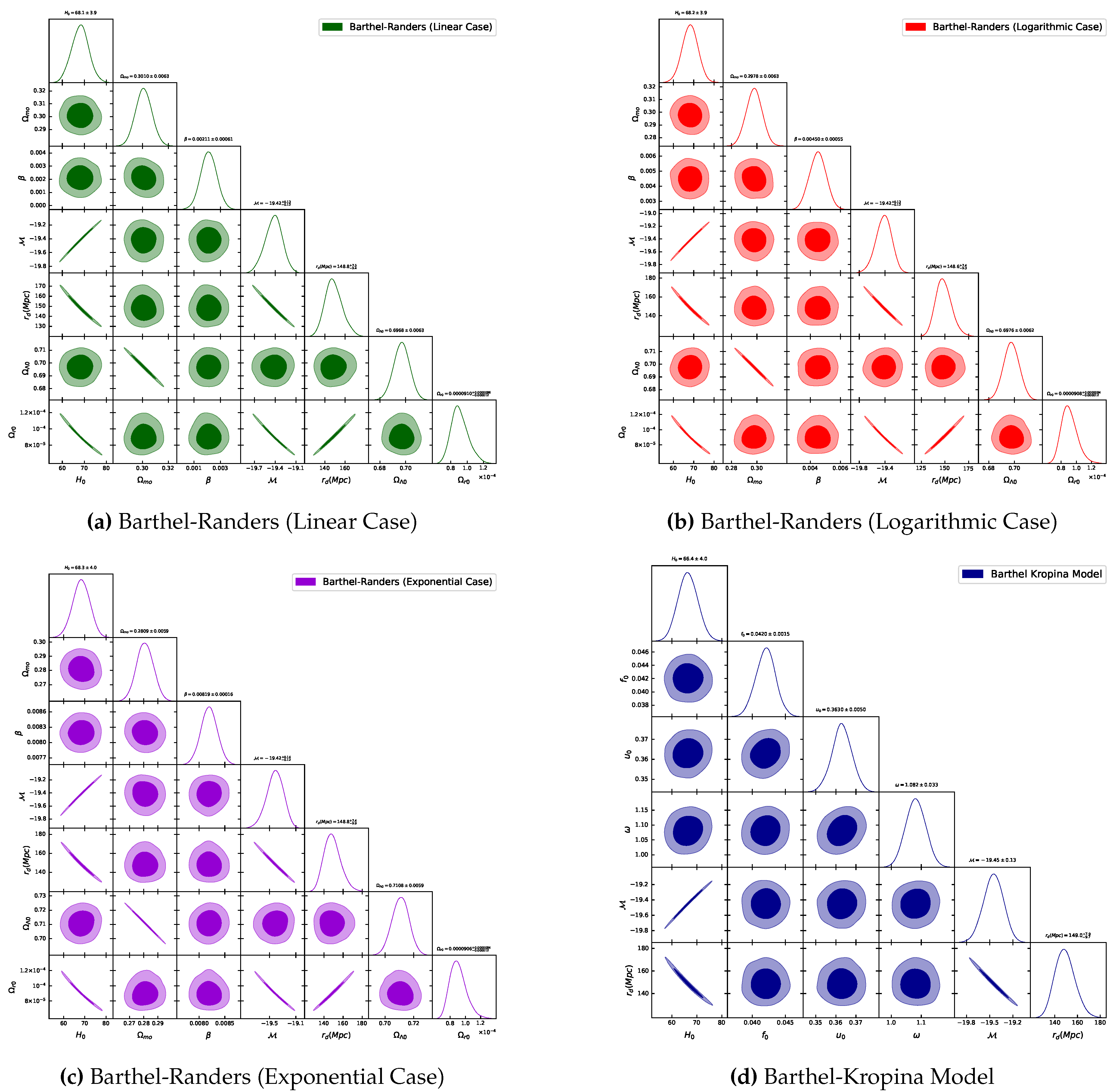
Table 2. Summary of the mean values and 95% credible intervals (2$\sigma$) for the parameters of the $\Lambda$CDM, Barthel-Randers, and Barthel-Kropina cosmological models.

Cosmological Models	Parameter	JOINT
$\Lambda$CDM Model	$H_0$	$68.1\pm 4.1$
	${\Omega }_{m0}$	$0.3040\pm 0.0064$
	$\mathcal{M}$	$-19.42\pm 0.12$
	$r_d$	$148.8\pm 7.6$
	${\Omega }_{\Lambda 0}$	$0.6960\pm 0.0064$
BR (Linear Case)	$H_0$	$68.1\pm 3.9$
	${\Omega }_{m0}$	$0.3010\pm 0.0063$
	$\beta$	$0.00211\pm 0.00061$
	$\mathcal{M}$	$-19.42\pm 0.12$
	$r_d$	$148.8\pm 7.5$
	${\Omega }_{\Lambda 0}$	$0.6968\pm 0.0063$
	${\Omega }_{r0}$	$(9.10\pm 1.20)\times {10}^{-5}$
BR (Logarithmic Case)	$H_0$	$68.1\pm 3.9$
	${\Omega }_{m0}$	$0.2978\pm 0.0063$
	$\beta$	$0.00450\pm 0.00055$
	$\mathcal{M}$	$-19.42\pm 0.13$
	$r_d$	$148.6\pm 7.4$
	${\Omega }_{\Lambda 0}$	$0.6976\pm 0.0062$
	${\Omega }_{r0}$	$(9.08\pm 1.20)\times {10}^{-5}$
BR (Exponential Case)	$H_0$	$68.3\pm 4.0$
	${\Omega }_{m0}$	$0.2809\pm 0.0059$
	$\beta$	$0.00819\pm 0.00016$
	$\mathcal{M}$	$-19.42\pm 0.14$
	$r_d$	$148.8\pm 7.4$
	${\Omega }_{\Lambda 0}$	$0.7108\pm 0.0059$
	${\Omega }_{r0}$	$(9.06\pm 1.20)\times {10}^{-5}$
Barthel-Kropina Model	$H_0$	$66.4\pm 4.0$
	$f_0$	$0.0420\pm 0.0015$
	$u_0$	$0.3630\pm 0.0050$
	$\omega$	$1.082\pm 0.033$
	$\mathcal{M}$	$-19.45\pm 0.13$
	$r_d$	$149.0\pm 7.9$

Table 2. Summary of the mean values and 95% credible intervals (2$\sigma$) for the parameters of the $\Lambda$CDM, Barthel-Randers, and Barthel-Kropina cosmological models.

Cosmological Models	Parameter	JOINT
$\Lambda$CDM Model	$H_0$	$68.1\pm 4.1$
	${\Omega }_{m0}$	$0.3040\pm 0.0064$
	$\mathcal{M}$	$-19.42\pm 0.12$
	$r_d$	$148.8\pm 7.6$
	${\Omega }_{\Lambda 0}$	$0.6960\pm 0.0064$
BR (Linear Case)	$H_0$	$68.1\pm 3.9$
	${\Omega }_{m0}$	$0.3010\pm 0.0063$
	$\beta$	$0.00211\pm 0.00061$
	$\mathcal{M}$	$-19.42\pm 0.12$
	$r_d$	$148.8\pm 7.5$
	${\Omega }_{\Lambda 0}$	$0.6968\pm 0.0063$
	${\Omega }_{r0}$	$(9.10\pm 1.20)\times {10}^{-5}$
BR (Logarithmic Case)	$H_0$	$68.1\pm 3.9$
	${\Omega }_{m0}$	$0.2978\pm 0.0063$
	$\beta$	$0.00450\pm 0.00055$
	$\mathcal{M}$	$-19.42\pm 0.13$
	$r_d$	$148.6\pm 7.4$
	${\Omega }_{\Lambda 0}$	$0.6976\pm 0.0062$
	${\Omega }_{r0}$	$(9.08\pm 1.20)\times {10}^{-5}$
BR (Exponential Case)	$H_0$	$68.3\pm 4.0$
	${\Omega }_{m0}$	$0.2809\pm 0.0059$
	$\beta$	$0.00819\pm 0.00016$
	$\mathcal{M}$	$-19.42\pm 0.14$
	$r_d$	$148.8\pm 7.4$
	${\Omega }_{\Lambda 0}$	$0.7108\pm 0.0059$
	${\Omega }_{r0}$	$(9.06\pm 1.20)\times {10}^{-5}$
Barthel-Kropina Model	$H_0$	$66.4\pm 4.0$
	$f_0$	$0.0420\pm 0.0015$
	$u_0$	$0.3630\pm 0.0050$
	$\omega$	$1.082\pm 0.033$
	$\mathcal{M}$	$-19.45\pm 0.13$
	$r_d$	$149.0\pm 7.9$

5. Comparing Barthel-Randers, Barthel-Kropina and $\Lambda$CDM Cosmological Models

After obtaining the mean parameter values from the MCMC simulations, we proceed to compare the predictions of the Barthel-Randers and Barthel-Kropina cosmological models with standard $\Lambda$CDM model. This comparison is essential to assess how well the Barthel-Randers and Barthel-Kropina framework replicates the observed cosmic expansion history.

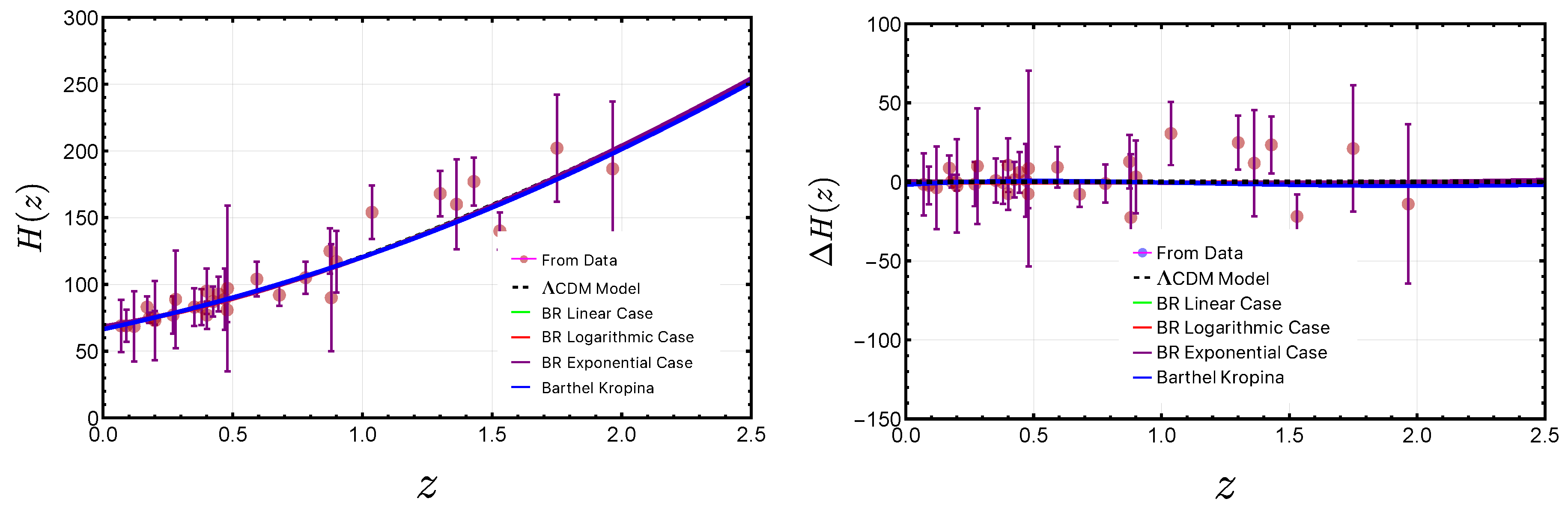
5.1. Evolution of the Hubble Parameter $H\left(z\right)$ and Hubble Residual $\Delta H\left(z\right)$

The Hubble parameter $H\left(z\right)$ characterizes the rate of cosmic expansion as a function of redshift z. Using the mean parameter values for each of the three Barthel-Randers models and Barthel-Kropina model, we compute $H\left(z\right)$ over a relevant redshift range and compare the results with those predicted by the $\Lambda$CDM model. We adopt the following form of the $\Lambda$CDM model for this comparison

$$H_{\Lambda \mathrm{CDM}}(z,H_0,{\Omega }_{m0},{\Omega }_{\Lambda 0})=H_0\sqrt{{\Omega }_{m0}{(1+z)}^3+{\Omega }_{\Lambda 0}},$$

where ${\Omega }_{m0}=0.304$, ${\Omega }_{\Lambda 0}=0.695$, and $H_0=68.1\mathrm{km}{\mathrm{s}}^{-1}{\mathrm{Mpc}}^{-1}$. To quantify the deviation between the Barthel-Randers models and $\Lambda$CDM, we define the Hubble residual as

$$\Delta H\left(z\right)=H_{\mathrm{Barthel}-\mathrm{Randers}\mathrm{Models}}\left(z\right)-H_{\Lambda \mathrm{CDM}}\left(z\right),$$

where $H_{\mathrm{Barthel}-\mathrm{Randers}\mathrm{Models}}\left(z\right)$ denotes the Hubble parameter predicted by the respective Barthel-Randers model. Similarly, for the Barthel-Kropina model, we define

$$\Delta H\left(z\right)=H_{\mathrm{Barthel}-\mathrm{Kropina}\mathrm{Model}}\left(z\right)-H_{\Lambda \mathrm{CDM}}\left(z\right),$$

where $H_{\mathrm{Barthel}-\mathrm{Kropina}\mathrm{Model}}\left(z\right)$ denotes the Hubble parameter predicted by the respective Barthel-Kropina model. Plotting both $H\left(z\right)$ and $\Delta H\left(z\right)$ for the Barthel-Randers models and Barthel-Kropina model allows us to visualize the distinct behaviors introduced by each model and assess their consistency with the standard cosmological framework. A small or nearly constant residual would indicate close agreement with $\Lambda$CDM, while significant deviations may point to possible extensions or alternatives to the standard model.

Figure 3. Comparison of the Barthel-Randers (Linear, Logarithmic, Exponential), Barthel-Kropina, with $\Lambda$CDM model. The left panel shows the evolution of the Hubble parameter $H\left(z\right)$ using mean MCMC values. The right panel shows the Hubble residuals $\Delta H\left(z\right)$, indicating deviations from the standard model.

Figure 3. Comparison of the Barthel-Randers (Linear, Logarithmic, Exponential), Barthel-Kropina, with $\Lambda$CDM model. The left panel shows the evolution of the Hubble parameter $H\left(z\right)$ using mean MCMC values. The right panel shows the Hubble residuals $\Delta H\left(z\right)$, indicating deviations from the standard model.

5.2. Cosmographic Analysis of Barthel-Randers and Barthel-Kropina Models

Cosmography provides a model-independent framework to describe the kinematic behavior of the Universe by expanding cosmological quantities in terms of redshift [170,171,172,173]. In this work, we apply this approach to analyze the deceleration and jerk parameters within the Barthel-Randers and Barthel-Kropina cosmological models, which modify standard cosmic dynamics through different geometrical correction terms.

5.2.1. Deceleration Parameter $q\left(z\right)$ and Jerk Parameter $j\left(z\right)$

The deceleration parameter $q\left(z\right)$ describes the acceleration or deceleration of the cosmic expansion and is defined as:

$$q\left(z\right)=-{\displaystyle \frac{1}{H^2\left(z\right)}}{\displaystyle \frac{dH\left(z\right)}{dz}}-1,$$

A negative value of $q\left(z\right)$ indicates that the Universe is undergoing accelerated expansion. Two important phase derived from $q\left(z\right)$ are the present-day deceleration parameter, $q_0=q(z=0)$, which describes the current rate of acceleration, and the transition redshift, $z_{\mathrm{tr}}$, defined by the condition $q\left(z_{\mathrm{tr}}\right)=0$, marking the point at which the Universe transitioned from decelerated to accelerated expansion. The jerk parameter $j\left(z\right)$ is a third-order cosmographic quantity defined as [174]:

$$j\left(z\right)={\displaystyle \frac{1}{H^3\left(z\right)}}{\displaystyle \frac{d^{2}H\left(z\right)}{d{z}^2}}.$$

which characterizes the rate of change of the acceleration. Importantly, in the standard $\Lambda$CDM model, the jerk parameter remains constant at $j\left(z\right)=1.$ Any deviation from this value can signal dynamics beyond the standard cosmological model. For the three Barthel-Randers models and the Barthel-Kropina model, we evaluate both the deceleration parameter $q\left(z\right)$ and the jerk parameter $j\left(z\right)$ numerically and assess their behavior across the redshift range.

Figure 4. Evolution of the deceleration parameter $q\left(z\right)$ and jerk parameter $j\left(z\right)$ for the Barthel-Randers (Linear, Logarithmic, Exponential), Barthel-Kropina, with $\Lambda$CDM model. The left panel shows the evolution of $q\left(z\right)$ as a function of redshift, while the right panel presents $j\left(z\right)$, showing deviations from the $\Lambda$CDM value $j=1$.

Figure 4. Evolution of the deceleration parameter $q\left(z\right)$ and jerk parameter $j\left(z\right)$ for the Barthel-Randers (Linear, Logarithmic, Exponential), Barthel-Kropina, with $\Lambda$CDM model. The left panel shows the evolution of $q\left(z\right)$ as a function of redshift, while the right panel presents $j\left(z\right)$, showing deviations from the $\Lambda$CDM value $j=1$.

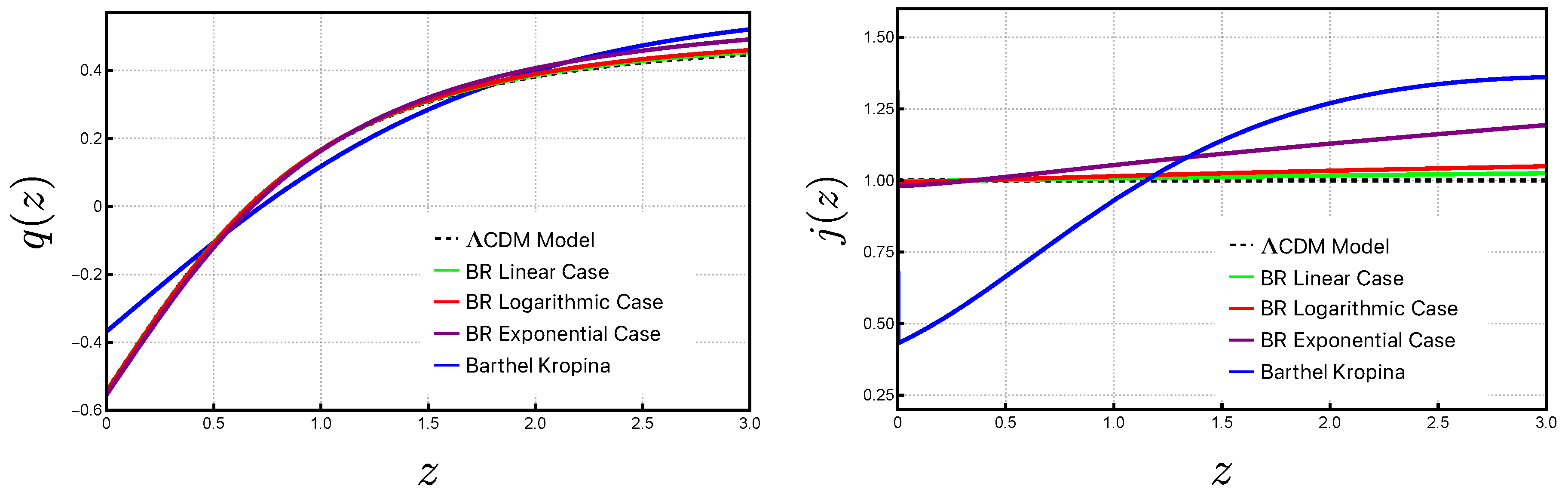
5.3. Statistical Assessment of Barthel-Randers and Barthel-Kropina Models

In this subsection, we apply a set of model selection criteria to evaluate the goodness-of-fit and model complexity of three variants of the Barthel-Randers cosmological models (Linear, Logarithmic, and Exponential) and Barthel-Kropina model. It is crucial to assess how well each models aligns with the data when compared to the $\Lambda$CDM model.

5.4. Goodness of Fit: ${\chi }^2$ and ${\chi }_{red}^2$

The primary measure of model fit is the chi-squared statistic, ${\chi }^2$, which quantifies the discrepancy between theoretical predictions and observational data. For a more normalized comparison, especially when models have different numbers of parameters, we compute the reduced chi-squared:

$${\chi }_{\mathrm{red}}^2={\displaystyle \frac{{\chi }_{\mathrm{tot}}^2}{\mathrm{DOF}}},$$

(123)

where ${\chi }_{\mathrm{tot}}^2$ is the total chi-squared value and DOF denotes the degrees of freedom, calculated as the number of data points minus the number of fitted parameters. A value of ${\chi }_{\mathrm{red}}^2\approx 1$ indicates a good statistical fit [175]. Lower values can suggest overfitting, while significantly higher values may reflect poor model performance.

5.4.1. Model Comparison Using AIC and BIC

In addition to chi-squared statistics, we apply information-theoretic criteria that account for both fit quality and model complexity. These include the Akaike Information Criterion (AIC) and the Bayesian Information Criterion (BIC), defined respectively as [176,177,178,179,180]:

$$\begin{array}{cc}\hfill \mathrm{AIC}& =-2log{\mathcal{L}}_{tot,max}+2\mathcal{P},\hfill \end{array}$$

(124)

$$\begin{array}{cc}\hfill \mathrm{BIC}& =-2log{\mathcal{L}}_{tot,max}+\mathcal{P}ln\left(\mathcal{N}\right),\hfill \end{array}$$

(125)

where $\mathcal{P}$ is the number of free parameters, $\mathcal{N}$ is the total number of data points used in the analysis and ${\mathcal{L}}_{tot,max}$ is the total maximum likelihood. In our analysis, the total number of data points used is the sum of three different observational datasets: $\mathcal{N}=1749$. For the model comparison, we note that the $\Lambda$CDM model has 4 free parameters, whereas the Barthel-Randers cosmological model has 5 free parameters, and the Barthel-Kropina model has 6 free parameters. These criteria penalize overly complex models to prevent overfitting. BIC generally applies a stricter penalty than AIC, especially in large datasets.

5.4.2. Relative Comparison: $\Delta$AIC and $\Delta$BIC

To directly compare the Barthel-Randers models with the $\Lambda$CDM model, we compute

$$\begin{array}{cc}\hfill \Delta \mathrm{AIC}& ={\mathrm{AIC}}_{\mathrm{Barthel}-\mathrm{Randers}\mathrm{Models}}-{\mathrm{AIC}}_{\Lambda \mathrm{CDM}\mathrm{Model}},\hfill \end{array}$$

(126)

$$\begin{array}{cc}\hfill \Delta \mathrm{BIC}& ={\mathrm{BIC}}_{\mathrm{Barthel}-\mathrm{Randers}\mathrm{Models}}-{\mathrm{BIC}}_{\Lambda \mathrm{CDM}\mathrm{Model}}.\hfill \end{array}$$

(127)

Similarly, for the comparison between the Barthel-Kropina model and the $\Lambda$CDM model, we compute

$$\begin{array}{cc}\hfill \Delta \mathrm{AIC}& ={\mathrm{AIC}}_{\mathrm{Barthel}-\mathrm{Kropina}\mathrm{Model}}-{\mathrm{AIC}}_{\Lambda \mathrm{CDM}\mathrm{Model}},\hfill \end{array}$$

(128)

$$\begin{array}{cc}\hfill \Delta \mathrm{BIC}& ={\mathrm{BIC}}_{\mathrm{Barthel}-\mathrm{Kropina}\mathrm{Model}}-{\mathrm{BIC}}_{\Lambda \mathrm{CDM}\mathrm{Model}}.\hfill \end{array}$$

(129)

According to the calibrated Jeffreys’ scales [181], these differences offer insight into model preference:

• $|\Delta \mathrm{AIC}|\le 2$: Comparable support.
• $4\le |\Delta \mathrm{AIC}|<10$: Considerably less support.
• $|\Delta \mathrm{AIC}|\ge 10$: Strongly disfavored.
• $|\Delta \mathrm{BIC}|\le 2$: Weak evidence against the model.
• $2<|\Delta \mathrm{BIC}|\le 6$: Moderate evidence against the model.
• $|\Delta \mathrm{BIC}|>6$: Strong evidence against the model.

A negative value of $\Delta \mathrm{AIC}$ or $\Delta \mathrm{BIC}$ indicates that the Barthel-Randers and Barthel-Kropina models are preferred over $\Lambda$CDM, whereas positive values suggest that the Barthel-Randers and Barthel-Kropina models are less favored.

5.4.3. p-Value Statistics

In our analysis, we also computed the p-value to assess the statistical significance of the fit for the Barthel-Randers cosmological models, calculated as follows:

$$p=1-{\mathcal{F}}_{{\chi }_{\min }^2}(\chi \mid \nu ),$$

where ${\mathcal{F}}_{{\chi }_{\min }^2}(\chi \mid \nu )$ is the cumulative distribution function (CDF) of the chi-squared distribution with $\nu$ degrees of freedom, and $\nu$ represents the number of data points minus the number of free parameters [182].

The p-value quantifies the likelihood of observing results as extreme as those seen in the data, assuming the null hypothesis holds true. A p-value smaller than 0.05 ($p<0.05$) indicates statistical significance, providing strong evidence against the null hypothesis and suggesting that the model is a good fit for the data. These corresponding statistical metrics (${\chi }_{\min }^2$, ${\chi }_{\mathrm{red}}^2$, AIC, BIC, $\Delta$AIC, $\Delta$BIC, and p-value) are computed and compared against the $\Lambda$CDM model. These statistical metrics ensure that both the goodness of fit and the complexity of each model are thoroughly evaluated, enabling a comprehensive statistical assessment of the Barthel-Randers model and Barthel-Kropina models in the context of cosmology.

Table 3. Summary of ${\chi }_{\mathrm{tot},min}^2$, ${\chi }_{\mathrm{red}}^2$, AIC, $\Delta$AIC, BIC, $\Delta$BIC, and p-value for the $\Lambda$CDM model and Barthel-Randers models (Linear, Logarithmic, Exponential), as well as the Barthel-Kropina model.

Model	${\mathbf{\chi }}_{\mathbf{tot}}^2$	${\mathit{\chi }}_{\mathbf{red}}^2$	AIC	$\mathit{\Delta }$AIC	BIC	$\mathit{\Delta }$BIC	p-value
$\Lambda$CDM Model	1802.34	1.032	1810.34	0.00	1832.20	0.00	0.165
BR (Linear Case)	1802.54	1.033	1812.54	2.20	1839.87	7.76	0.160
BR (Logarithmic Case)	1802.89	1.033	1812.89	2.55	1840.22	8.01	0.159
BR (Exponential Case)	1805.15	1.035	1815.15	4.81	1842.48	10.27	0.150
Barthel-Kropina Model	1782.19	1.022	1794.19	$-16.14$	1826.99	$-5.21$	0.251

Table 3. Summary of ${\chi }_{\mathrm{tot},min}^2$, ${\chi }_{\mathrm{red}}^2$, AIC, $\Delta$AIC, BIC, $\Delta$BIC, and p-value for the $\Lambda$CDM model and Barthel-Randers models (Linear, Logarithmic, Exponential), as well as the Barthel-Kropina model.

Model	${\mathbf{\chi }}_{\mathbf{tot}}^2$	${\mathit{\chi }}_{\mathbf{red}}^2$	AIC	$\mathit{\Delta }$AIC	BIC	$\mathit{\Delta }$BIC	p-value
$\Lambda$CDM Model	1802.34	1.032	1810.34	0.00	1832.20	0.00	0.165
BR (Linear Case)	1802.54	1.033	1812.54	2.20	1839.87	7.76	0.160
BR (Logarithmic Case)	1802.89	1.033	1812.89	2.55	1840.22	8.01	0.159
BR (Exponential Case)	1805.15	1.035	1815.15	4.81	1842.48	10.27	0.150
Barthel-Kropina Model	1782.19	1.022	1794.19	$-16.14$	1826.99	$-5.21$	0.251

6. Synthesis of the Results, and Their Discussion

In the present Section we will discuss the main results obtained from the comparison of the present cosmological models with observations, and with the standard $\Lambda$CDM paradigm.

6.1. MCMC Results

Figure 2 presents the corner plot comparing the Barthel-Randers and Barthel-Kropina cosmological models. Figure 2a–c shows the corner plots for the Linear, Logarithmic, and Exponential cases of the Barthel-Randers model, respectively. Figure 2d shows the corner plot for the Osculating Barthel-Kropina dark energy model. The diagonal panels illustrate the one-dimensional marginalized posterior distributions for each parameter, highlighting their most probable values. The off-diagonal panels depict the two-dimensional marginalized contour plots, showing the 68% and 95% confidence intervals.

These contour plots also reveal correlations or degeneracies between parameters. One can observe that the predicted values of $H_0$ in the case of $\Lambda$CDM and the Barthel-Randers models (Linear, Logarithmic, and Exponential cases) are close to those predicted by the DESI results: $H_0^{\mathrm{DESI}\mathrm{DR}1}=(68.52\pm 0.62)\mathrm{km}{\mathrm{s}}^{-1}{\mathrm{Mpc}}^{-1}$ and $H_0^{\mathrm{DESI}\mathrm{DR}2}=(68.17\pm 0.28)\mathrm{km}{\mathrm{s}}^{-1}{\mathrm{Mpc}}^{-1}$. On the other hand, the predicted value of $H_0$ in the case of the Osculating Barthel-Kropina dark energy model aligns more closely with the Planck estimation: $H_0^{\mathrm{Planck}}=(67.4\pm 0.5)\mathrm{km}{\mathrm{s}}^{-1}{\mathrm{Mpc}}^{-1}$.

The predicted values of $r_d$ in all the models are consistent with the Planck estimation, $r_d^{\mathrm{Planck}}=(147.09\pm 0.26)\mathrm{Mpc}$. Although the central value of our predicted $H_0$ aligns well with the estimations from Planck, DESI DR1, and DESI DR2, the associated uncertainty is noticeably larger. This increased uncertainty primarily stems from the inclusion of the full SNe Ia dataset, which, while providing a more comprehensive observational foundation, also introduces larger statistical and systematic errors. A similar trend is observed in the inferred value of the sound horizon at the drag epoch, $r_d$, where our model yields a larger uncertainty compared to the Planck determination. Additionally, we adopt the full covariance matrix for the CC analysis as provided by [159]. For comparison, the current constraints on the f$\Lambda$CDM model using the CC data from Moresco et al. yield: $H_0=66.2_{-3.9}^{+3.8}\mathrm{km}{\mathrm{s}}^{-1}{\mathrm{Mpc}}^{-1}$ when systematics due to SPS models are not included, and $H_0=66.0_{-5.6}^{+5.5}\mathrm{km}{\mathrm{s}}^{-1}{\mathrm{Mpc}}^{-1}$ when the full set of systematic uncertainties is taken into account.

The predicted value of the present-day matter density parameter in the case of the $\Lambda$CDM model, as well as the Linear case of the Barthel-Randers model, is lower than the Planck estimation, ${\Omega }_{m0}^{\mathrm{Planck}}=0.315\pm 0.007,$ and is closer to the values predicted by DESI DR1 and DESI DR2, ${\Omega }_{m0}^{\mathrm{DESI}\mathrm{DR}1}=0.295\pm 0.015\mathrm{and}{\Omega }_{m0}^{\mathrm{DESI}\mathrm{DR}2}=0.2975\pm 0.0086.$

Similarly, the predicted value of ${\Omega }_{m0}$ in the Logarithmic case of the Barthel-Randers model is also in good agreement with the DESI DR1 and DR2 estimations. In contrast, the Exponential case of the Barthel-Randers model predicts a matter density parameter that is lower than the values reported by both DESI DR1 and DR2. It is interesting to observe that the $\Lambda$CDM model, as well as the Linear, Logarithmic, and Exponential cases of the Barthel-Randers model, predict a present-day dark energy density parameter, ${\Omega }_{\Lambda 0}$, that is greater than the value predicted by the Planck estimation: ${\Omega }_{\Lambda 0}^{\mathrm{Planck}}=0.685\pm 0.007.$

6.2. Hubble parameter and Hubble residual results

Figure 3 shows the evolution of the Hubble function and the Hubble residuals for the Linear, Logarithmic, and Exponential cases of the Barthel-Randers model, as well as the Barthel-Kropina model. These are compared with the predictions from the $\Lambda$CDM model and CC measurements. The left panel shows that at high redshift ($z>0.7$), all the considered models deviate noticeably from the $\Lambda$CDM model. However, these deviations are not significant. At low redshift ($z<0.7$), each model aligns closely with the $\Lambda$CDM predictions.

On the right plane we can also observe similar behavior in the Hubble residual plots, where each model shows a slight deviation from the $\Lambda$CDM model at high redshift. However, at low redshift, all models exhibit behavior that closely matches the $\Lambda$CDM predictions. All considered models (Barthel-Randers variants and Barthel-Kropina) closely follow $\Lambda$CDM at low redshifts, indicating consistency with current observations. Their mild deviations at higher redshifts ($z>0.7$) suggest a potentially different early Universe expansion history, offering alternative insights that may help address cosmological tensions such as the Hubble tension.

6.3. Cosmographic Results

Figure 4 shows the evolution of the cosmography parameters for the Linear, Logarithmic, and Exponential cases of the Barthel-Randers model, along with the Barthel-Kropina model, compared to the $\Lambda$CDM model. The left panel shows the evolution of the deceleration parameter, $q\left(z\right)$.

Notably, the Barthel-Kropina model exhibits a distinct evolution compared to both the standard $\Lambda$CDM model and the Barthel-Randers variants. At present time ($z=0$), all Barthel-Randers variants and $\Lambda$CDM predict a deceleration parameter of approximately $q_0\approx -0.511$, while the Barthel-Kropina model predicts a less negative value of $q_0\approx -0.366$. We also analyze an important cosmological feature: the transition redshift $z_{\mathrm{tr}}$.

For the $\Lambda$CDM model, the transition from decelerated to accelerated expansion occurs at $z_{\mathrm{tr}}^{\Lambda \mathrm{CDM}}\approx 0.623.$ The Barthel-Randers variants exhibit slightly later transitions: $z_{\mathrm{tr}}^{\mathrm{BR}\mathrm{Linear}}\approx 0.610,z_{\mathrm{tr}}^{\mathrm{BR}\mathrm{Logarithmic}}\approx 0.607,\mathrm{and}{z}_{\mathrm{tr}}^{\mathrm{BR}\mathrm{Exponential}}\approx 0.606.$

In contrast, the Barthel-Kropina model shows a significantly earlier transition at $z_{\mathrm{tr}}^{\mathrm{Barthel}-\mathrm{Kropina}}\approx 0.723.$ While at high redshift all models show deviations from the $\Lambda$CDM model in their evolution, these deviations are not significant. The right panel shows the evolution of the jerk parameter for each model. At the present time ($z=0$), all variants of the Barthel-Randers models exhibit good agreement with the $\Lambda$CDM model. Although each variant predicts a slightly different value for the jerk parameter, these deviations are not significant. Moreover, the Barthel-Kropina model shows a substantial deviation from the other models, predicting a present-day jerk value of $j_0^{\mathrm{Barthel}-\mathrm{Kropina}}\approx 0.448.$

At high redshift, all variants of the Barthel-Randers models, as well as the Barthel-Kropina model, deviate from the predictions of the $\Lambda$CDM model.

6.4. Statistical Results

Table 3 presents a comparative analysis of the Linear Case, Logarithmic Case, and Exponential Case of the Barthel-Randers model, as well as the Barthel-Kropina model, against the $\Lambda$CDM model, using several statistical metrics. The ${\chi }_{\mathrm{tot},min}^2$ value, a measure of the goodness of fit, for the $\Lambda$CDM model is 1802.34. The Barthel-Randers models (Linear, Logarithmic, and Exponential cases) show similar total ${\chi }_{\mathrm{tot},min}^2$ values ranging from 1802.54 to 1805.15, which are slightly higher than that of the $\Lambda$CDM model. The Barthel Kropina model shows the lowest ${\chi }_{\mathrm{tot},min}^2$ value of 1782.19. This indicates that, in terms of overall goodness of fit, the Barthel Kropina model provides the best fit, while the Barthel-Randers models perform slightly worse than the $\Lambda$CDM model.

The ${\chi }_{\mathrm{red}}^2$ value provides insight into the goodness of fit adjusted for the number of data points and parameters in the model. The $\Lambda$CDM model has a ${\chi }_{\mathrm{red}}^2$ of 1.032, which is very close to the Barthel-Randers models, all of which have values slightly above 1.033. The lowest ${\chi }_{\mathrm{red}}^2$ value is from the Barthel Kropina model (1.022), indicating that it is marginally the best in terms of adjusting for the complexity of the model and fitting the data well.

The AIC is a measure of the relative quality of a model, accounting for both the goodness of fit and the number of parameters. The $\Lambda$CDM model has an AIC of 1810.34. The Barthel-Randers models (Linear, Logarithmic, and Exponential) have AIC values around 1812.54, 1812.89, and 1815.15, which are higher by 2.20, 2.55, and 4.81, respectively, compared to the $\Lambda$CDM model, indicating a slightly worse balance between fit and model complexity. The Barthel Kropina model has the lowest AIC value of 1794.19, which is 16.14 lower than the $\Lambda$CDM model. According to the AIC criterion, the Barthel Kropina model provides the best balance between fit and complexity, while the Barthel-Randers models perform slightly worse than the $\Lambda$CDM model.

The BIC is another metric for model selection, similar to AIC but with a stronger penalty for the number of parameters. The $\Lambda$CDM model has a BIC of 1832.20, which is lower than the Barthel-Randers models but slightly higher than the Barthel Kropina model. The Barthel-Randers models show BIC values between 1839.87 and 1842.48, with an increase of approximately 7.76 to 10.27 compared to the $\Lambda$CDM model. The Barthel Kropina model has the lowest BIC of 1826.99, a decrease of 5.21 compared to the $\Lambda$CDM model. This suggests that the Barthel Kropina model is the best according to the BIC criterion, while the Barthel-Randers models perform worse than the $\Lambda$CDM model.

The p-value indicates the statistical significance of the model in terms of explaining the data. The $\Lambda$CDM model has a p-value of 0.165, indicating that the model is statistically significant at a conventional level (i.e., it cannot be rejected at the 5% significance level). All the other models (Barthel-Randers Linear, Logarithmic, Exponential, and Barthel Kropina) have p-values ranging from 0.160 to 0.251, which are slightly higher or comparable, suggesting that none of the models can be rejected at the 5% significance level. The p-values imply that all models, including the base $\Lambda$CDM model, are statistically significant in explaining the data.

The Barthel Kropina model outperforms the $\Lambda$CDM model in terms of goodness of fit, AIC, and BIC, offering a better balance between fit and model complexity. The Barthel-Randers models (Linear, Logarithmic, Exponential), however, perform slightly worse than the $\Lambda$CDM model in this updated comparison.

Despite these improvements, all models, including the $\Lambda$CDM model, are statistically significant, with p-values indicating that none of them should be rejected. In terms of simplicity, however, the $\Lambda$CDM model remains the most straightforward and easiest to interpret. Therefore, while the Barthel Kropina model appears to be the most favorable overall, the differences between the models are relatively small, and all offer comparable statistical significance.

7. Discussions and Final Remarks

One of the fundamental assumptions, and results, of present day physics is that the gravitational interaction can be successfully described only in geometric terms. However, which geometry can best described gravity is still a matter of debate. The initial Riemannian framework of general relativity was extended to include geometries with nonmetricity, torsion, or both. Teleparallel geometries have also been considered as potential candidates for the description of gravity.

In the present work we have briefly reviewed some recent advances in the application of another geometric framework that could provide some insight into the understanding of the gravitational force, namely, Finsler geometry, and its various particular cases. In Finsler geometry, instead of the point x of Riemann geometry, the metric depends also on an internal degree of freedom y, which is often physically interpreted as velocity. Hence, the y dependence is the essential characteristic of Finsler spaces, and the presence of this internal degrees of freedom opens some new perspective on the physical interpretation of the Finsler geometric theories. Thus, Finsler geometries are generally anisotropic and nonlocal, and these properties significantly enlarge the possibilities of the physical applications.

On the other hand, from a physical point of view it is natural to assume that in some specific physical processes the internal vector y becomes a function of x. Such specific situations may occur if we interpret y as describing space-time fluctuations, and we perform an averaging over it, according to the rule $〈\varphi \left(x\right)〉=\int \varphi (x,y)f\left(y\right)d^{4}y$, where $f\left(y\right)$ is a specific distribution function of y[48]. Hence, Finsler geometry with $\widehat{g}\left(x\right)={\left.g(x,y)\right|}_{y=Y\left(x\right)}$ has a deep physical origin, which points towards interesting physical consequences. The averaging, or the osculating process leads to a reduction of a Finsler geometry F to a corresponding Riemann geometry. The interpretation of the vector y as related to some quantum effects, like the vacuum fluctuation, is also supported by the fact that generally in $(\alpha ,\beta )$ type gravitational theories the matter energy-momentum tensor is not conserved. The most natural physical interpretation of this result is related to the possibility of particle production from the Finslerian vacuum in an expanding Universe, an effect that is also specific to quantum field theories in curved spacetimes [140,141,142,143,144]. Hence, Finslerian type gravitational theories can offer a glimpse on the structure and classical limit of quantum field theories in Riemann geometries.

In our presentation we have concentrated on a specific class of osculating geometries, the osculating $(\alpha ,\beta )$ geometries, which have the remarkable property that their Barthel connection is the Levi-Civita connection. This property allows a significant simplification of the mathematical formalism, which becomes easily tractable by using the standard methods of Riemannian geometry. The osculating $(\alpha ,\beta )$ type theories can be interpreted as two metric theories. First, we have the Finsler metric function $F(\alpha ,\beta )$, which generates its own metric, while $\alpha$ is a Riemannian metric given a priori. For cosmological applications the FLRW metric can be adopted as the Riemann metric $\alpha$, and we assume that this is the physical metric in which the real, observable gravitational processes take place. However, the Finsler metric $\widehat{g}\left(x\right)=g(x,Y\left(x\right))$ has also an important imprint on gravitation, since its presence induces new terms in the gravitational field equations. We have investigated the effects of these new terms from a cosmological perspective only, by interpreting them as describing an effective dark energy that is responsible for the late acceleration of the Universe.

An important test of a cosmological model is represented by its consistency with the observations. We have used three observational datasets (Cosmic Chronometers, Type Ia Supernovae, Baryon Acoustic Oscillations) to perform a detailed analysis, and comparison of the Barthel-Randers, Barthel-Kropina and $\lambda$CDM models. Generally, one can appreciate that all the considered models give a good description of the observational data, but important differences still do appear between the various Finslerian approaches, and the $\Lambda$CDM model. The differences do appear, for example, in the prediction of the critical redshift $z_{crit}$ at which the transition from deceleration to acceleration occurs, with the Barthel-Randers models predicting a value of $z_{crit}$ of the order of $z_{crit}\approx 0.60$, while in the Barthel-Kropina cosmology $z_{crit}\approx 0.72$. Significant differences do appear in the present values of the deceleration parameter $q\left(0\right)$, which in the Barthel-Kropina cosmology takes the value $q\left(0\right)\approx -0.37$, while in $\Lambda$CDM and Barthel-Randers models it has the value $q\left(0\right)\approx -0.50$. Moreover, at redshifts $z>3$, the predictions of all considered models show significant differences with respect to each other. Hence, cosmological observations at high redshift will give the possibility of discriminating between the various cosmological models based on modified gravity theory constructed with the help of Finsler (and other) geometries.

The main goal of the present review is to draw attention to the possibilities offered by Finsler geometry in the explanation of the cosmological phenomena, and to give a brief introduction to the existing results in a very specific, and simple class, of this very complex geometry. We have presented in some detail the generalized Friedmann cosmological equations, and the general theoretical framework in which cosmological models can be constructed. We would like to point out that from the point of view of calculations, the derivation of the field equations and of the evolution equations in these particular geometries are no more complicated than those in standard general relativity. This is related especially to the important fact that the connection in osculating point Finsler geometries is, for the $(\alpha ,\beta )$ metrics, the Barthel connection, which has the same mathematical form as the Levi-Civita connection. In our review we have presented some basic theoretical tools that can be used for the further exploration of the applications of Finsler geometry in the description of gravitational phenomena.

References

- Weyl, H. Gravitation und Elektrizität. In Sitzungsberichte der Königlich Preussischen Akademie der Wissenschaften zu Berlin, 1918 ed.; Königlich Preussische Akademie: Berlin, Germany, 1918; pp. 465–480. [Google Scholar]
- Weyl, H. Space, Time, Matter; Dover Publications: New York, NY, USA, 1952. [Google Scholar]
- Finsler, P. Über Kurven und Flächen in allgemeinen Räumen. Dissertation, University of Göttingen, Germany, 1918; reprinted by Birkhäuser: Basel, Switzerland, 1951.
- Einstein, A. Die Feldgleichungen der Gravitation. In Sitzungsberichte der Königlich Preussischen Akademie der Wissenschaften zu Berlin, 1915 ed.; Königlich Preussische Akademie: Berlin, Germany, 1915; pp. 844–847. [Google Scholar]
- Einstein, A. Die Grundlage der allgemeinen Relativitätstheorie. Annalen der Physik 1916, 49, 769–822. [Google Scholar] [CrossRef]
- Hilbert, D. Die Grundlagen der Physik. Nachrichten von der Gesellschaft der Wissenschaften zu Göttingen, Mathematisch-Physikalische Klasse 1915, 395–407.
- Scholz, E. Weyl Geometry in Late 20th Century Physics. In Beyond Einstein: Perspectives on Geometry, Gravitation, and Cosmology in the Twentieth Century; Rowe, D.E., Sauer, T., Walter, S.A., Eds.; Springer: New York, NY, USA, 2018; pp. 261–360. [Google Scholar]
- Riemann, B. Über die Hypothesen, welche der Geometrie zu Grunde liegen. Abhandlungen der Königlichen Gesellschaft der Wissenschaften zu Göttingen 1868, 13, 133–150. [Google Scholar]
- Chern, S.S. Finsler Geometry Is Just Riemannian Geometry without the Quadratic Restriction. Notices of the American Mathematical Society 1996, 43, 959–963. [Google Scholar]
- Rund, H. The Differential Geometry of Finsler Spaces; Springer-Verlag: Berlin, Germany, 1959. [Google Scholar]
- Asanov, G.S. Finsler Geometry, Relativity and Gauge Theories; D. Reidel Publishing Company: Dordrecht, The Netherlands, 1985. [Google Scholar]
- Bejancu, A. Finsler Geometry and Applications; Ellis Horwood: New York, NY, USA, 1990. [Google Scholar]
- Bao, D.; Chern, S.-S.; Shen, Z. An Introduction to Riemann-Finsler Geometry; Springer-Verlag: New York, NY, USA, 2000. [Google Scholar]
- Shen, Y.-B.; Shen, Z. Introduction to Modern Finsler Geometry; World Scientific: Singapore, 2016. [Google Scholar]
- Will, C.M. The Confrontation between General Relativity and Experiment. Living Reviews in Relativity 2014, 17, 4. [Google Scholar] [CrossRef] [PubMed]
- Abbott, B.P. et al. (LIGO Scientific Collaboration and Virgo Collaboration). Observation of Gravitational Waves from a Binary Black Hole Merger. Physical Review Letters 2016, 116, 061102. [Google Scholar] [CrossRef] [PubMed]
- Abbott, R. et al. (LIGO Scientific Collaboration and Virgo Collaboration). GW190814: Gravitational Waves from the Coalescence of a 23 Solar Mass Black Hole with a 2.6 Solar Mass Compact Object. Astrophysical Journal Letters 2020, 896, L44. [Google Scholar] [CrossRef]
- Cartan, É. Sur les variétés à connexion affine et la théorie de la relativité généralisée. Annales de l’École Normale Supérieure 1924, 41, 1–25. [Google Scholar] [CrossRef]
- Cartan, É. Sur les variétés à connexion affine et la théorie de la relativité généralisée. Annales de l’École Normale Supérieure 1925, 42, 17–88. [Google Scholar] [CrossRef]
- Weitzenböck, R. Invariantentheorie; Noordhoff: Groningen, The Netherlands, 1923. [Google Scholar]
- Ehlers, J.; Pirani, F.A.E.; Schild, A. The Geometry of Free Fall and Light Propagation. General Relativity and Gravitation, 44, 1587 (2012).
- Linnemann, N.; Read, J. Constructive Axiomatics in Spacetime Physics Part I: Walkthrough to the Ehlers-Pirani-Schild Axiomatisation. Preprint, arXiv:2112.14063 [gr-qc], 2021.
- Adlam, E.; Linnemann, N.; Read, J. Constructive Axiomatics in Spacetime Physics Part II: Constructive Axiomatics in Context. Preprint, arXiv:2211.05672 [gr-qc], 2022.
- Adlam, E.; Linnemann, N.; Read, J. Constructive Axiomatics in Spacetime Physics Part III: A Constructive Axiomatic Approach to Quantum Spacetime. Preprint, arXiv:2208.07249 [gr-qc], 2022.
- Pfeifer, C. Finsler Spacetime Geometry in Physics. International Journal of Geometric Methods in Modern Physics, 16 (suppl. 02), 1941004 (2019).
- Randers, G. On an Asymmetrical Metric in the Four-Space of General Relativity. Physical Review, 59, 195 (1941).
- Ingarden, R. On the Geometrically Absolute Optical Representation in the Electron Microscope. Travaux de la Société des Sciences et des Lettres de Wrocław, Série B, 45, 3 (1957).
- Miron, R. The Geometry of Ingarden Spaces. Reports on Mathematical Physics, 54, 131 (2004).
- Tavernelli, I. On the Geometrization of Quantum Mechanics. Annals of Physics, 371, 239 (2016).
- Tavernelli, I. On the Self-Interference in Electron Scattering: Copenhagen, Bohmian and Geometrical Interpretations of Quantum Mechanics. Annals of Physics, 393, 447 (2018).
- Liang, S.-D.; Sabau, S.V.; Harko, T. Finslerian Geometrization of Quantum Mechanics in the Hydrodynamical Representation. Physical Review D, 100, 105012 (2019).
- Tavernelli, I. Gravitational Quantum Dynamics: A Geometrical Perspective. Foundations of Physics, 51, 46 (2021).
- Hohmann, M.; Pfeifer, C.; Voicu, N. The Kinetic Gas Universe. European Physical Journal C, 80, 809 (2020).
- Pfeifer, C.; Voicu, N.; Friedl-Szász, A.; Popovici-Popescu, E. From Kinetic Gases to an Exponentially Expanding Universe. Preprint, arXiv:2504.08062 [gr-qc], 2025.
- Rätzel, D.; Rivera, S.; Schuller, F.P. Geometry of Physical Dispersion Relations. Physical Review D, 83, 044047 (2011).
- Duval, C. Finsler Spinoptics. Communications in Mathematical Physics, 283, 701–727 (2008).
- Schreck, M. Classical Lagrangians and Finsler Structures for the Nonminimal Fermion Sector of the Standard-Model Extension. Physical Review D, 93, 105017 (2016).
- Edwards, B.R.; Kostelecký, V.A. Riemann–Finsler Geometry and Lorentz-Violating Scalar Fields. Physics Letters B, 786, 319–326 (2018).
- Horváth, J.I. A Geometrical Model for the Unified Theory of Physical Fields. Physical Review, 80, 901 (1950).
- Horváth, J.I.; Moór, A. Entwicklung einer einheitlichen Feldtheorie begründet auf die Finslersche Geometrie. Zeitschrift für Physik, 131, 548 (1952).
- Takano, Y. Gravitational Field in Finsler Spaces. Lettere al Nuovo Cimento, 10, 747 (1974).
- Takano, Y. Variation Principle in Finsler Spaces. Lettere al Nuovo Cimento, 11, 486 (1974).
- Asanov, G.S. Finslerian Extension of General Relativity. Foundations of Physics, 11, 137 (1981).
- Asanov, G.S. Finsler Geometry, Relativity and Gauge Theories; D. Reidel: Dordrecht, The Netherlands, 1985. [Google Scholar]
- Asanov, G.S. Finslerian Solution for Static Spherically Symmetric Gravitational Field. Fortschritte der Physik, 39, 185 (1991).
- Asanov, G.S. Finslerian Extension of Schwarzschild Metric. Fortschritte der Physik, 40, 667 (1992).
- Miron, R.; Anastasiei, M. Vector Bundles, Lagrange Spaces, and Applications to the Theory of Relativity; Editura Academiei Române: Bucharest, Romania, 1987. (in Romanian) [Google Scholar]
- Ikeda, S. Advanced Studies in Applied Geometry; Seizansha: Sagamihara, Japan, 1995. [Google Scholar]
- Rutz, S.F. A Finsler Generalisation of Einstein’s Vacuum Field Equations. General Relativity and Gravitation, 25, 1139 (1993).
- Li, X.; Chang, Z. Exact Solution of Vacuum Field Equation in Finsler Spacetime. Chinese Physics C, 34, 28 (2010).
- Hohmann, M.; Pfeifer, C.; Voicu, N. Finsler Gravity Action from Variational Completion. Physical Review D, 100, 064035 (2019).
- Riess, A.G.; et al. (Supernova Search Team). Observational Evidence from Supernovae for an Accelerating Universe and a Cosmological Constant. Astronomical Journal, 116, 1009 (1998).
- Perlmutter, S.; et al. (Supernova Cosmology Project). Measurements of Ω and Λ from 42 High-Redshift Supernovae. Astrophysical Journal, 517, 565 (1999).
- Knop, R.A.; et al. New Constraints on ΩM, ΩΛ, and w from an Independent Set of Eleven High-Redshift Supernovae Observed with HST. Astrophysical Journal, 598, 102 (2003).
- Amanullah, R.; et al. Spectra and Light Curves of Six Type Ia Supernovae at 0.511 < z < 1.12 and the Union2 Compilation. Astrophysical Journal, 716, 712 (2010).
- Weinberg, D.H.; Mortonson, M.J.; Eisenstein, D.J.; Hirata, C.; Riess, A.G.; Rozo, E. Observational Probes of Cosmic Acceleration. Physics Reports, 530, 87 (2013).
- Einstein, A. Kosmologische Betrachtungen zur allgemeinen Relativitätstheorie. Sitzungsberichte der Königlich Preußischen Akademie der Wissenschaften (Berlin), part 1, 142–152 (1917).
- Weinberg, S. The Cosmological Constant Problem. Reviews of Modern Physics, 61, 1 (1989).
- Salucci, P.; Turini, N.; Di Paolo, C. Paradigms and Scenarios for the Dark Matter Phenomenon. Universe, 6, 118 (2020).
- Alam, S.; et al. (BOSS Collaboration). The Clustering of Galaxies in the Completed SDSS-III Baryon Oscillation Spectroscopic Survey: Cosmological Analysis of the DR12 Galaxy Sample. Monthly Notices of the Royal Astronomical Society, 470, 2617 (2017).
- Abbott, T.M.C.; et al. (DES Collaboration). Dark Energy Survey Year 1 Results: Cosmological Constraints from Galaxy Clustering and Weak Lensing. Physical Review D, 98, 043526 (2018).
- Tanabashi, M.; et al. (Particle Data Group). Review of Particle Physics. Physical Review D, 98, 030001 (2018).
- Aghanim, N.; et al. (Planck Collaboration). Planck 2018 Results. VI. Cosmological Parameters. Astronomy & Astrophysics, 641, A6 (2020).
- Martel, H.; Shapiro, P.R.; Weinberg, S. Likely Values of the Cosmological Constant. Astrophysical Journal, 492, 29 (1998).
- Weinberg, S. The Cosmological Constant Problems. In Sources and Detection of Dark Matter and Dark Energy in the Universe; Cline, D.B., Ed.; Springer-Verlag: Berlin, Germany, 2001; p. 18, arXiv:astro-ph/0005265. [Google Scholar]
- Lake, M.J. A New Approach to the Cosmological Constant Problems. SciPost Physics Proceedings, 4, 014 (2021).
- Riess, A.G.; Casertano, S.; Yuan, W.; Macri, L.M.; Scolnic, D. Large Magellanic Cloud Cepheid Standards Provide Foundation for the Determination of the Hubble Constant and Stronger Evidence for Physics Beyond LCDM. Astrophysical Journal, 876, 85 (2019).
- Huang, C.D.; Riess, A.G.; Yuan, W.; Macri, L.M.; Zakamska, N.L.; Casertano, S.; Whitelock, P.A.; Hoffmann, S.L.; Filippenko, A.V.; Scolnic, D. Hubble Space Telescope Observations of Mira Variables in the SN Ia Host NGC 1559: An Alternative Candle to Measure the Hubble Constant. Astrophysical Journal, 889, 5 (2020).
- Pesce, D.W.; et al. The Megamaser Cosmology Project. XIII. Combined Hubble Constant Constraints. Astrophysical Journal Letters, 891, L1 (2020).
- Harko, T.; Lobo, F.S.N. Beyond Einstein’s General Relativity: Hybrid Metric-Palatini Gravity and Curvature-Matter Couplings. International Journal of Modern Physics D, 29, 2030008 (2020).
- Haghani, Z.; Harko, T.; Sepangi, H.R.; Shahidi, S. Weyl-Cartan-Weitzenböck Gravity as a Generalization of Teleparallel Gravity. Journal of Cosmology and Astroparticle Physics, 10, 061 (2012).
- Haghani, Z.; Harko, T.; Sepangi, H.R.; Shahidi, S. Weyl-Cartan-Weitzenböck Gravity through Lagrange Multiplier. Physical Review D, 88, 044024 (2013).
- Nester, J.M.; Yo, H.-J. Symmetric Teleparallel General Relativity. Chinese Journal of Physics, 37, 113 (1999).
- Beltrán Jiménez, J.; Heisenberg, L.; Koivisto, T. Coincident General Relativity. Physical Review D, 98, 044048 (2018).
- D’Agostino, R.; Luongo, O. Growth of Matter Perturbations in Nonminimal Teleparallel Dark Energy. Physical Review D, 98, 124013 (2018).
- Fontanini, M.; Huguet, E.; Le Delliou, M. Teleparallel Gravity (TEGR) as a Gauge Theory. Physical Review D, 99, 064006 (2019).
- Koivisto, T.; Tsimperis, G. The Spectrum of Teleparallel Gravity. Universe, 5, 80 (2019).
- Pereira, J.G.; Obukhov, Y.N. Gauge Structure of Teleparallel Gravity. Universe, 5, 139 (2019).
- Blixt, D.; Hohmann, M.; Pfeifer, C. On the Gauge Fixing in the Hamiltonian Analysis of General Teleparallel Theories. Universe, 5, 143 (2019).
- Coley, A.A.; van den Hoogen, R.J.; McNutt, D.D. Symmetry and Equivalence in Teleparallel Gravity. Journal of Mathematical Physics, 61, 072503 (2020).
- Haghani, Z.; Khosravi, N.; Shahidi, S. The Weyl–Cartan Gauss–Bonnet Gravity. Classical and Quantum Gravity, 32, 215016 (2015).
- Sotiriou, T.P.; Faraoni, V. f(R) Theories of Gravity. Reviews of Modern Physics, 82, 451 (2010).
- De Felice, A.; Tsujikawa, S. f(R) Theories. Living Reviews in Relativity, 13, 3 (2010).
- Cai, Y.F.; Capozziello, S.; De Laurentis, M.; Saridakis, E.N. f(T) Teleparallel Gravity and Cosmology. Reports on Progress in Physics, 79, 106901 (2016).
- Nojiri, S.; Odintsov, S.D.; Oikonomou, V.K. Modified Gravity Theories on a Nutshell: Inflation, Bounce and Late-Time Evolution. Physics Reports, 692, 1 (2017).
- Odintsov, S.D.; Oikonomou, V.K.; Giannakoudi, I.; Fronimos, F.P.; Lymperiadou, E.C. Recent Advances in Inflation. Symmetry, 15, 1701 (2023).
- Basilakos, S.; Stavrinos, P. Cosmological Equivalence between the Finsler–Randers Space-Time and the DGP Gravity Model. Physical Review D, 87, 043506 (2013).
- Exirifard, Q. Cosmological Implications of Modified Gravity Induced by Quantum Metric Fluctuations. Journal of Cosmology and Astroparticle Physics, 11, 026 (2015).
- Silva, J.E.G.; Maluf, R.V.; Almeida, C.A.S. Effective Gravitational Equations on a Brane in Teleparallel Gravity. Physics Letters B, 766, 263 (2017).
- Papagiannopoulos, G.; Basilakos, S.; Paliathanasis, A.; Savvidou, S.; Stavrinos, P.C. Dynamics and Observational Constraints in Scalar–Tensor Theories in Finsler–Randers Spacetime. Classical and Quantum Gravity, 34, 225008 (2017).
- Papagiannopoulos, G.; Basilakos, S.; Paliathanasis, A.; Pan, S.; Stavrinos, P. Finsler–Randers Cosmology: Dynamical Analysis and Growth of Matter Perturbations. European Physical Journal C, 80, 816 (2020).
- Raushan, R.; Chaubey, S. Finslerian Cosmological Model with Bulk Viscosity in Bianchi Type-I Space-Time. European Physical Journal Plus, 135, 228 (2020).
- Triantafyllopoulos, A.; Basilakos, S.; Kapsabelis, E.; Stavrinos, P.C. Finsler–Randers Cosmology: Dynamical Analysis and Growth of Matter Perturbations. European Physical Journal C, 80, 1200 (2020).
- Kapsabelis, E.; Triantafyllopoulos, A.; Basilakos, S.; Stavrinos, P.C. Dynamical Analysis of a Scalar Field Cosmology in Finsler–Randers Spacetime. European Physical Journal C, 81, 990 (2021).
- Kapsabelis, E.; Kevrekidis, P.G.; Stavrinos, P.C.; Triantafyllopoulos, A. Finsler–Randers Cosmology: Dynamical Analysis and Growth of Matter Perturbations. European Physical Journal C, 82, 1098 (2022).
- Nekouee, Z.; Narasimhamurthy, S.K.; Manjunatha, H.M.; Srivastava, S.K. Finslerian Cosmological Model with Bulk Viscosity in Bianchi Type-I Space-Time. European Physical Journal Plus, 137, 1388 (2022).
- Feng, W.; Yang, W.; Jiang, B.; Wang, Y.; Han, T.; Wu, Y. Observational Constraints on Finslerian Cosmology. International Journal of Modern Physics D, 32, 2350029 (2023).
- Das, P.D.; Debnath, U. Finslerian Cosmological Model with Bulk Viscosity in Bianchi Type-I Space-Time. European Physical Journal C, 83, 821 (2023).
- Triantafyllopoulos, A.; Kapsabelis, E.; Stavrinos, P.C. Finsler–Randers Cosmology: Dynamical Analysis and Growth of Matter Perturbations. Universe, 10, 26 (2024).
- Kapsabelis, E.; Saridakis, E.N.; Stavrinos, P.C. Finsler–Randers Cosmology: Dynamical Analysis and Growth of Matter Perturbations. European Physical Journal C, 84, 538 (2024).
- Praveen, J.; Narasimhamurthy, S.K.; Yashwanth, B.R. Finslerian Cosmological Model with Bulk Viscosity in Bianchi Type-I Space-Time. European Physical Journal C, 84, 597 (2024).
- Liu, J.; Wang, R.; Gao, F. Finsler–Randers Cosmology: Dynamical Analysis and Growth of Matter Perturbations. Universe, 10, 302 (2024).
- Nekouee, Z.; Narasimhamurthy, S.K.; Pourhassan, B.; Pacif, S.K.J. Finslerian Cosmological Model with Bulk Viscosity in Bianchi Type-I Space-Time. Annals of Physics, 470, 169787 (2024).
- Nekouee, Z.; Chaudhary, H.; Narasimhamurthy, S.K.; Pacif, S.K.J.; Malligawad, M. Finsler–Randers Cosmology: Dynamical Analysis and Growth of Matter Perturbations. Journal of High Energy Astrophysics, 44, 19 (2024).
- Praveen, J.; Narasimhamurthy, S.K. Finslerian Cosmological Model with Bulk Viscosity in Bianchi Type-I Space-Time. Journal of High Energy Astrophysics, 44, 300 (2024).
- Yashwanth, B.R.; Narasimhamurthy, S.K.; Praveen, J.; Malligawad, M. Finsler–Randers Cosmology: Dynamical Analysis and Growth of Matter Perturbations. European Physical Journal C, 84, 1272 (2024).
- Praveen, J.; Narasimhamurthy, S.K. Finslerian Cosmological Model with Bulk Viscosity in Bianchi Type-I Space-Time. New Astronomy, 119, 102404 (2025).
- Ikeda, S.; Saridakis, E.N.; Stavrinos, P.C.; Triantafyllopoulos, A. Cosmology of Lorentz Fiber-Bundle Induced Scalar-Tensor Theories. Physical Review D, 100, 124035 (2019).
- Fuster, A.; Pabst, C.; Pfeifer, C. Berwald Spacetimes and Very Special Relativity. Physical Review D, 98, 084062 (2018).
- Hohmann, M.; Pfeifer, C.; Voicu, N. Cosmological Finsler Spacetimes. Universe, 6, 65 (2020).
- Hama, R.; Harko, T.; Sabau, S.V.; Shahidi, S. Cosmological Evolution and Dark Energy in Osculating Barthel–Randers Geometry. European Physical Journal C, 81, 742 (2021).
- Hama, R.; Rattanasak, R.; Harko, T.; Sabau, S.V. Dark Energy and Accelerating Cosmological Evolution from Osculating Barthel–Kropina Geometry. European Physical Journal C, 82, 385 (2022).
- Bouali, A.; Chaudhary, H.; Hama, R.; Harko, T.; Sabau, S.V.; San Martín, M. Cosmological Tests of the Osculating Barthel–Kropina Dark Energy Model. European Physical Journal C, 83, 121 (2023).
- Hama, R.; Harko, T.; Sabau, S.V. Conformal Gravitational Theories in Barthel–Kropina-Type Finslerian Geometry and Their Cosmological Implications. European Physical Journal C, 83, 1030 (2023).
- Tavakol, R.K.; Van den Bergh, N. Finsler Spaces and the Underlying Geometry of Space-Time. Physics Letters A, 112, 23 (1985).
- Tavakol, R.K. Geometry of Spacetime and Finsler Geometry. International Journal of Modern Physics A, 24, 1678 (2009).
- Javaloyes, M.A.; Sánchez, M. On the Definition and Examples of Finsler Metrics. Annali della Scuola Normale Superiore di Pisa, Classe di Scienze, 13, 813 (2014).
- Yoshikawa, R.; Sabau, S.V. Kropina Metrics and Zermelo Navigation on Riemannian Manifolds. Geometriae Dedicata, 171, 119 (2014).
- Kropina, V.K. On Projective Finsler Spaces with a Metric of Special Form. Nauchnye Doklady Vysshei Shkoly, Fiziko-Matematicheskie Nauki, 2, 38 (1959).
- Kropina, V.K. On Projective Finsler Spaces with a Metric of Special Form. Uchenye Zapiski Arkhangelskogo Gosudarstvennogo Pedagogicheskogo Instituta, 4, 111 (1959).
- Matsumoto, M. On C-Reducible Finsler Spaces. Tensor, New Series, 24, 29–37 (1972).
- Matsumoto, M. Theory of Finsler Spaces with (α, β)-Metric. Reports on Mathematical Physics, 31, 43–83 (1992).
- Bácsó, S.; Cheng, X.; Shen, Z. Curvature Properties of (α, β)-Metrics. Advanced Studies in Pure Mathematics, 48, 73–110 (2007).
- Antonelli, P.L.; Ingarden, R.S.; Matsumoto, M. The Theory of Sprays and Finsler Spaces with Applications in Physics and Biology; Kluwer Academic Publishers: Dordrecht, The Netherlands, 1993. [Google Scholar]
- Miron, R.; Hrimiuc, D.; Shimada, H.; Sabau, S.V. The Geometry of Hamilton and Lagrange Spaces; Kluwer Academic Publishers: Dordrecht, The Netherlands, 2001. [Google Scholar]
- Yoshikawa, R.; Sabau, S.V. Kropina Metrics and Zermelo Navigation on Riemannian Manifolds. Publicationes Mathematicae Debrecen, 84, 483–499 (2014).
- Sabau, S.V.; Shibuya, K.; Yoshikawa, R. Geodesics on Strong Kropina Manifolds. European Journal of Mathematics, 3, 1172–1224 (2017).
- Heefer, S.; Pfeifer, C.; van Voorthuizen, J.; Fuster, A. On the Metrizability of m-Kropina Spaces with Closed Null One-Form. Journal of Mathematical Physics, 64, 022502 (2023).
- Heefer, S. Berwald m-Kropina Spaces of Arbitrary Signature: Metrizability and Ricci-Flatness. Journal of Mathematical Physics, 65, 122502 (2024).
- Barthel, W. Über eine Geometrische Deutung der Automorphen Funktionen. Mathematische Zeitschrift, 58, 358 (1953).
- Barthel, W. Zur Theorie der Automorphen Funktionen. Archiv der Mathematik, 4, 346 (1953).
- Ingarden, R.S.; Tamássy, L. The Point Finsler Spaces and Their Physical Applications in Electron Optics and Thermodynamics. Mathematical and Computer Modelling, 20, 93 (1994).
- Nazim, A. Über Finslersche Räume. Dissertation, München, Germany, 1936.
- Varga, O. Zur Herleitung des Invarianten Differentials in Finslerschen Räumen. Monatshefte für Mathematik und Physik, 50, 165 (1941).
- Harko, T. Thermodynamic Interpretation of the Generalized Gravity Models with Geometry–Matter Coupling. Physical Review D, 90, 044067 (2014).
- Bertolami, O.; Böhmer, C.G.; Harko, T.; Lobo, F.S.N. Extra Force in f(R) Modified Theories of Gravity. Physical Review D, 75, 104016 (2007).
- Harko, T.; Lobo, F.S.N.; Otalora, G.; Saridakis, E.N. Nonminimal Torsion–Matter Coupling Extension of f(T) Gravity. Physical Review D, 89, 124036 (2014).
- Parker, L. Particle Creation in Expanding Universes. Physical Review Letters, 21, 562 (1968).
- Parker, L. Quantized Fields and Particle Creation in Expanding Universes. I. Physical Review, 183, 1057 (1969).
- Zeldovich, Ya.B.; Starobinsky, A.A. Particle Production and Vacuum Polarization in an Anisotropic Gravitational Field. Zhurnal Éksperimental’noĭ i Teoreticheskoĭ Fiziki, 61, 2161 (1971); [Soviet Physics JETP, 34, 1159 (1972)].
- Parker, L. Particle Creation in Isotropic Cosmologies. Physical Review Letters, 28, 705 (1972); Erratum: Physical Review Letters, 28, 1497 (1972).
- Fulling, S.A.; Parker, L.; Hu, B.L. Conformal Energy-Momentum Tensor in Curved Spacetime: Adiabatic Regularization and Renormalization. Physical Review D, 10, 3905 (1974).
- Parker, L. Particle Creation and Particle Number in an Expanding Universe. Journal of Physics A: Mathematical and Theoretical, 45, 374023 (2012).
- Prigogine, I.; Geheniau, J.; Gunzig, E.; Nardone, P. Thermodynamics of Cosmological Matter Creation. Proceedings of the National Academy of Sciences of the USA, 85, 7428 (1988).
- Calvão, M.O.; Lima, J.A.S.; Waga, I. On the Thermodynamics of Matter Creation in Cosmology. Physics Letters A, 162, 223 (1992).
- Su, J.; Harko, T.; Liang, S.-D. Thermodynamics in Modified Gravity Theories with Geometry–Matter Coupling. Advances in High Energy Physics, 2017, 7650238 (2017).
- Lima, J.A.S.; Baranov, I.P. Gravitationally Induced Particle Production: Thermodynamics and Kinetic Theory. Physical Review D, 90, 043515 (2014).
- Saridakis, E.N.; González-Díaz, P.F.; Sigüenza, C.L. Unified Dark Energy Thermodynamics: Varying w and the −1-Crossing. Classical and Quantum Gravity, 26, 165003 (2009).
- Bernardo, J. M. Reference Prior Distributions for Bayesian Inference. J. R. Stat. Soc. B 1979, 41, 113–127. [Google Scholar] [CrossRef]
- Joyce, J. Bayes’ Theorem. In The Stanford Encyclopedia of Philosophy, Fall 2021 ed.; Zalta, E.N., Ed.; Stanford University: Stanford, CA, USA, 2021. [Google Scholar]
- Lewis, A. GetDist: A Python Package for Analysing Monte Carlo Samples. arXiv 2019, arXiv:1910.13970. [Google Scholar]
- Jimenez, R.; Loeb, A. Constraining Cosmological Parameters Based on Relative Galaxy Ages. Astrophys. J. 2002, 573, 37–51. [Google Scholar] [CrossRef]
- Moresco, M. Raising the Bar: New Constraints on the Hubble Parameter with Cosmic Chronometers at z ∼2. Mon. Not. R. Astron. Soc. 2015, 450, L16–L20. [Google Scholar] [CrossRef]
- Moresco, M.; Pozzetti, L.; Cimatti, A.; Jimenez, R.; Maraston, C.; Verde, L.; Thomas, D.; Citro, A.; Tojeiro, R.; Wilkinson, D. A 6% Measurement of the Hubble Parameter at z ∼0.45: Direct Evidence of the Epoch of Cosmic Re-acceleration. J. Cosmol. Astropart. Phys. 2016, 2016, 014. [Google Scholar] [CrossRef]
- Vagnozzi, S.; Loeb, A.; Moresco, M. Eppur è Piatto? The Cosmic Chronometers Take on Spatial Curvature and Cosmic Concordance. Astrophys. J. 2021, 908, 84. [Google Scholar] [CrossRef]
- Moresco, M.; Jimenez, R.; Verde, L.; Cimatti, A.; Pozzetti, L. Setting the Stage for Cosmic Chronometers. II. Impact of Stellar Population Synthesis Models Systematics and Full Covariance Matrix. Astrophys. J. 2020, 898, 82. [Google Scholar] [CrossRef]
- Brout, D.; Scolnic, D.; Popovic, B.; Riess, A. G.; Carr, A.; Zuntz, J.; Kessler, R.; Davis, T. M.; Hinton, S.; Jones, D.; et al. The Pantheon+ analysis: Cosmological constraints. Astrophys. J. 2022, 938, 110. [Google Scholar] [CrossRef]
- Astier, P.; Guy, J.; Regnault, N.; Pain, R.; Aubourg, E.; Balam, D.; Basa, S.; Carlberg, R.; Fabbro, S.; Fouchez, D.; et al. The supernova legacy survey: measurement of ω, ω and from the first year data set. Astron. Astrophys. 2006, 447, 31–48. [Google Scholar] [CrossRef]
- Conley, A.; Guy, J.; Sullivan, M.; Regnault, N.; Astier, P.; Balland, C.; Basa, S.; Carlberg, R.; Fouchez, D.; Hardin, D.; et al. Supernova constraints and systematic uncertainties from the first three years of the supernova legacy survey. Astrophys. J. Suppl. Ser. 2010, 192(1), 1.
- Karim, M. A.; Aguilar, J.; Ahlen, S.; Alam, S.; Allen, L.; Prieto, C. A.; Alves, O.; Anand, A.; Andrade, U.; Armengaud, E.; Aviles, A. DESI DR2 Results II: Measurements of Baryon Acoustic Oscillations and Cosmological Constraints. arXiv preprint 2025, arXiv:2503.14738, March 18, 2025.
- Pogosian, L.; Zhao, G.-B.; Jedamzik, K. Recombination-independent determination of the sound horizon and the Hubble constant from BAO. Astrophys. J. Lett. 2020, 904, L17. [Google Scholar] [CrossRef]
- Jedamzik, K.; Pogosian, L.; Zhao, G.-B. Why reducing the cosmic sound horizon alone can not fully resolve the Hubble tension. Commun. Phys. 2021, 4, 123. [Google Scholar] [CrossRef]
- Pogosian, L.; Zhao, G.-B.; Jedamzik, K. A consistency test of the cosmological model at the epoch of recombination using DESI BAO and Planck measurements. Astrophys. J. Lett. 2024, 973, L13. [Google Scholar] [CrossRef]
- Lin, W.; Chen, X.; Mack, K.J. Early universe physics insensitive and uncalibrated cosmic standards: Constraints on Ωm and implications for the Hubble tension. Astrophys. J. 2021, 920, 159. [Google Scholar] [CrossRef]
- Vagnozzi, S. Seven hints that early-time new physics alone is not sufficient to solve the Hubble tension. Universe 2023, 9, 393. [Google Scholar] [CrossRef]
- H. Chaudhary, L. Csillag, and T. Harko, "Semi-Symmetric Metric Gravity: A Brief Overview," Universe 10, 419 (2024).
- Cattoën, C.; Visser, M. Cosmographic Hubble fits to the supernova data. Phys. Rev. D 2008, 78, 063501. [Google Scholar] [CrossRef]
- Visser, M.; Cattoën, C. Cosmographic analysis of dark energy. In Dark Matter In Astrophysics And Particle Physics; Klapdor-Kleingrothaus, H.V., Krivosheina, I.V., Eds.; World Scientific Publishing Co. Pte. Ltd.: Singapore, 2009; pp. 287–300. [Google Scholar]
- Visser, M. Cosmography: Cosmology without the Einstein equations. Gen. Relativ. Gravit. 2005, 37, 1541. [Google Scholar] [CrossRef]
- Luongo, O. Cosmography with the Hubble parameter. Mod. Phys. Lett. A 2011, 26, 1459. [Google Scholar] [CrossRef]
- Visser, M. Jerk, snap and the cosmological equation of state. Class. Quantum Gravity 2004, 21, 2603. [Google Scholar] [CrossRef]
- Andrae, R.; Schulze-Hartung, T.; Melchior, P. Dos and don’ts of reduced chi-squared; arXiv preprint arXiv:1012.3754, 2010.
- Liddle, A.R. Information criteria for astrophysical model selection. Mon. Not. R. Astron. Soc. Lett. 2007, 377, L74. [Google Scholar] [CrossRef]
- Vrieze, S.I. Model selection and psychological theory: A discussion of the differences between the Akaike information criterion (AIC) and the Bayesian information criterion (BIC). Psychol. Methods 2012, 17, 228. [Google Scholar] [CrossRef]
- Tan, M.Y.J.; Biswas, R. The reliability of the Akaike information criterion method in cosmological model selection. Mon. Not. R. Astron. Soc. 2012, 419, 3292. [Google Scholar] [CrossRef]
- Arevalo, F.; Cid, A.; Moya, J. AIC and BIC for cosmological interacting scenarios. Eur. Phys. J. C 2017, 77, 1. [Google Scholar] [CrossRef]
- Burnham, K.P.; Anderson, D.R. Model Selection and Multimodel Inference, 2nd ed.; Springer: New York, NY, USA, 2010. [Google Scholar]
- Jeffreys, H. The Theory of Probability; Oxford University Press: Oxford, UK, 1998. [Google Scholar]
- Andrade, C. The P value and statistical significance: Misunderstandings, explanations, challenges, and alternatives; Indian Journal of Psychological Medicine, 41(3), 210–215, 2019.