
Submitted:
06 May 2025
Posted:
07 May 2025
You are already at the latest version
Abstract
Background: Classification trees (CTs) are widely used machine learning algorithms with growing applications in clinical research, especially for risk stratification. Their ability to generate interpretable decision rules makes them attractive to healthcare professionals. This review provides an accessible yet rigorous overview of CT methodology for clinicians, highlighting their utility through a case study addressing the "obesity paradox" in critically ill patients.
Methods: We describe key methodological aspects of CTs, including model development, pruning, validation, and classification types (simple, ensemble, and hybrid). Using data from the ENPIC study, which assessed artificial nutrition in ICU patients, we applied various CT approaches—CART, CHAID, and XGBoost—and compared them with logistic regression. SHAP values were used to interpret ensemble models.
Results: CTs allowed for identification of optimal cut-off points in continuous variables and revealed complex, non-linear interactions among predictors. Although the obesity paradox was not confirmed in the full cohort, CTs uncovered a specific subgroup in which obesity was associated with reduced mortality. The ensemble model (XGBoost) achieved the best predictive performance (highest AUC), though at the expense of interpretability.
Conclusions: CTs are valuable tools in clinical epidemiology, complementing traditional models by uncovering hidden patterns and enhancing risk stratification. While ensemble models offer superior predictive accuracy, their complexity necessitates interpretability techniques such as SHAP. CT-based approaches can guide personalized medicine but require cautious interpretation and external validation.
Keywords:
classification trees
; machine learning
; prediction modelling
; intensive care unit
; obesity paradox
1. Introduction
This work aims to provide an overview of the methodology of classification trees (CT), offering a perspective directed at clinical professionals interested in risk models. A technical yet accessible language has been used so that the content can be understood without requiring extensive methodological knowledge. For readers interested in a deeper understanding of the topic, we provide bibliographic references that we consider most suitable for further exploration, including examples related to nutrition-related problems.
Our focus is limited to classification trees that generate decision rules essential for establishing relationships between variables and identifying groups of patients with specific characteristics. CTs belong to a family of machine learning algorithms that use tree-like structures to support decision-making. This review is accompanied by a real-data application example to illustrate the utility and features of CTs.
1.1. Concept of a Classification Tree
A CT is the graphical representation of a series of decision rules. Starting from a root node, which includes all cases, the tree branches into different “child” nodes containing subgroups of cases. The splitting criterion, also known as branching criterion, is optimally determined after examining the values of all included predictor variables [1]. CTs are a form of supervised machine learning in which the algorithm is provided with records that include predictor variables and the outcome variable. These algorithms function by reducing classification error until the optimal CT is found [2].
1.2. Phases in the Construction of a Classification Tree
To illustrate the process of constructing a CT, we use the CART (Classification and Regression Tree) model as a reference. This process can be divided into several phases [4]:
Phase 1 – Tree Development: From the root node, the most appropriate variable is identified to split the node into two child nodes by establishing an optimal cut-off point if the variable is continuous. Each child node is subsequently split following the same methodology. A supervised machine learning model is used, with all records including predictor variables and the outcome variable submitted to the algorithm.
Phase 2 – Tree Growth Stopping Criteria: Tree development can continue until terminal nodes contain only a single case, or when the value of the dependent variable is the same for all cases within a node. Additional criteria, such as a minimum number of cases per node, can be defined to prevent excessive branching.
Phase 3 – Tree Pruning: A CT developed using the aforementioned method tends to be overly complex and branched, which may lead to overfitting the training dataset. Removing superfluous branches results in a simpler tree with better generalizability. The pruning process uses predefined cost-complexity criteria to eliminate branches that add more complexity than effectiveness. Supervised learning aims to reduce classification error.
Phase 4 – Selection of the Optimal CT: Selecting the optimal CT requires an internal validation system. This can be achieved by randomly splitting the sample into a training set and a validation set, or by applying cross-validation techniques. Cross-validation divides the dataset into subsets—e.g., 10 partitions using 9 for training and 1 for validation in a recursive process.
A final CT includes the decision rules that generate a probability for the event of interest, such as mortality or disease diagnosis.
1.3. Use of Classification Trees in Medicine
CTs have been used in medicine since their inception. The main tasks assigned to them include: generating decision rules for diagnosis, selecting variables based on their importance, determining cut-off points for continuous variables, and identifying clinical relationships among variables [5]. CT algorithms select the most relevant variables, their order of appearance in tree branching, and the optimal cut-off points [2]. The interpretability of decision rules makes CTs attractive for use in clinical settings [6].
A review of bibliographic databases reveals an exponential increase in publications using CT methodology, supporting their ongoing relevance in medical problems [6]. In the past two decades, the widespread adoption of machine learning techniques, including CTs, has further promoted their use [7].
We reference several studies that develop risk models using CTs and provide clear explanations of their methodological construction, such as a model for serious fall injury in older adults [8], or risk stratification in critically ill patients [9]. CTs have also been applied in nutrition, such as malnutrition detection [10], identifying the relationship between frailty and diet quality indicators [11], or predicting dropout from psychological treatment in bariatric surgery candidates [12].
1.4. Types of Classification Trees
There are many types of CTs [1,2]. Broadly, they can be divided into three main types (see Table 1): simple models that generate a single CT, ensemble models that use multiple CTs to improve accuracy, and hybrid models that combine CTs with other machine learning techniques, such as fuzzy logic or artificial neural networks [13].
Different types of simple CTs vary based on their stopping criteria, pruning methods, and procedures for selecting the optimal tree [9]. The most commonly used simple models include CART, CHAID, C4.5, and ctree [14,15,16,17,18]. Table 1 shows their specifications and the available software for implementation [19,20,21,22]. Notably, CART-type trees perform well with small datasets, which explains their continued use in limited data scenarios [9].
Other types of simple CTs, such as FACT (Fast and Accurate Classification Tree), QUEST (Quick Unbiased and Efficient Statistical Tree), CRUISE (Classification Rule with Unbiased Interaction Selection and Estimation), GUIDE (Generalized Unbiased Interaction Detection and Estimation), and Bayesian trees, have shown specific advantages in particular patient groups [2].
In general, model fitting parameters—called hyperparameters—include the tree's maximum depth (branching levels), the minimum number of cases per terminal node, and the internal validation method used (e.g., training-validation split or cross-validation). Each simple CT model may require specific additional hyperparameters for proper functioning [1,2,9].
Ensemble models will be discussed in a separate section. Hybrid models, such as those combining CTs with artificial neural networks or fuzzy logic, require more advanced methodological development [13].
1.5. Advantages and Disadvantages of Classification Trees
Although we have already mentioned several advantages and disadvantages of CTs, they can be summarized as follows [1,2,3,4,5]:
Advantages:
Non-parametric models
- -
- Can handle all variable types (continuous, ordinal, categorical)
- -
- Easy to interpret, with clinically meaningful decision rules
- -
- No additional calculations required to determine individual patient risk
- -
- Perform variable selection and establish variable hierarchy
- -
- Identify optimal cut-off points for continuous variables
- -
- Detect relationships among variables without assuming independence
- -
- Less affected by outliers or missing values
Disadvantages:
- -
- Risk of overfitting and limited generalizability
- -
- High sensitivity to data, leading to model instability
- -
- Complex trees may lose interpretability
- -
- Require specific software and development methodology
- -
- Many CT types exist, and the most suitable one for a specific problem may not be obvious in advance
In summary, it is necessary to strike a balance between the advantage of interpretability through decision rules and the methodological rigor required for their use.
2. ENPIC Study and the Obesity Paradox
We next describe the dataset used in this study, conducting a post hoc analysis of the ENPIC study (Evaluation of Practical Nutrition Practices in the Critical Care Patient), applying classification tree (CT) methodology to explore the obesity paradox [23].
2.1. The ENPIC Study
When providing artificial nutrition to critically ill patients, the goal is to optimize caloric and protein intake. Studies like ENPIC aim to address questions about how to improve this process [24,25,26].
The objective of the ENPIC study was to evaluate compliance with recommendations for specialized nutritional-metabolic treatment of critically ill patients and to assess the influence of nutritional therapy on mortality in this population [25]. It was a multicentre study including ICU patients requiring artificial nutrition, whether enteral or parenteral. The study sample included 525 patients.
2.2. The Obesity Paradox
The concept of the “obesity paradox” was first described in patients undergoing percutaneous coronary interventions, where improved survival was observed among overweight and obese individuals [27].
The obesity paradox suggests that obesity may exert a protective effect in certain diseases, leading to better survival outcomes [27].
Its presence in critically ill patients remains controversial [28]. Some authors argue that the phenomenon can be explained by selection bias and confounding, due to inadequate adjustment for variables involved in the obesity–mortality relationship [29,30,31].
A study published in this journal using the ENPIC dataset—Nutrition Therapy in Critically Ill Patients with Obesity—reported differences among BMI groups in some of the analysed characteristics, as shown in Table 2 [23].
This table presents the general characteristics, nutritional therapy, and outcomes of ICU patients stratified by body mass index (BMI) categories. It reveals demographic differences across BMI groups (normal weight, overweight, and obese). There is a non-significant trend toward lower 28-day mortality in obese patients, raising the question of whether the paradox might be present in this cohort.
The findings suggest that building a mortality risk model requires adjustment for patient-related factors (age, sex, BMI group), nutritional status based on Subjective Global Assessment (SGA), disease severity according to the APACHE II score (Acute Physiology and Chronic Health disease Classification System II) [32], and daily caloric (Kcal/kg/day) and protein (g/kg/day) intake. If the paradox is present, obesity would emerge as a protective factor.
We performed a multiple logistic regression (LR) model using the selected variables and calculated odds ratios (95% CI). Table 3 shows the model, which indicates that factors independently associated with 28-day mortality are older age, higher APACHE II score, malnutrition, and lower protein intake.
The obesity paradox was not detected in this model, as the odds ratio for obesity was not statistically significant. Given the limited sample size and the LR model used, we cannot confirm the presence of the paradox. Classification trees may uncover interactions or relationships not easily detected through traditional regression methods.
In the following sections, we apply CTs to the ENPIC dataset to illustrate methodological aspects and explore the potential presence of the obesity paradox.
3. Use of Classification Trees to Determine Cut-off Points
Continuous variables cannot be arbitrarily categorized. Typically, literature-based criteria or statistical methods are used to justify selected cut-off points.
Classification trees can be used to identify cut-off points in continuous variables and convert them into categorical ones—for example, to define score thresholds for diagnosing heart failure in patients with pleural effusion [33].
Other examples in nutrition-related contexts include determining a TNF-α cut-off related to HbA1c levels using a CHAID tree [34] or defining walking speed thresholds indicative of severe mobility limitations in sarcopenic patients using a CART tree [35].
In our paradox example, we employed a CHAID tree to determine cut-off points for Age and APACHE II score. Figure 1 shows that the selected age and APACHE II groups for categorization can be justified using classification trees.
4. Use of Classification Trees to Identify Relationships Between Variables
As mentioned earlier, one advantage of classification trees is their ability to detect relationships between variables. These relationships are often non-linear. Identifying such associations without assuming independence—and grouping patients based on these patterns—is essential for understanding how risk factors operate differently across subgroups [28].
In our example, previous research has suggested that exploring the obesity paradox requires stratifying patients by nutritional status [28]. In Figure 2, using a CART model, we observe that the risk of mortality is influenced by malnutrition. Among patients without malnutrition, the obese subgroup shows lower mortality, which may suggest that the paradoxical effect is detectable only in non-malnourished patients.
5. Multivariable Risk Models Using Classification Trees
A multivariable classification tree (CT) model can select only the most informative variables, establish a hierarchy, determine optimal cut-off points to categorize continuous variables, and indicate relationships between variables, resulting in a set of decision rules [6,9].
In the obesity paradox example, we included in the CT the same variables used in the logistic regression (LR) model (see Table 2). The CART-type classification tree model discarded caloric intake and sex. Figure 3 shows the classification tree with its decision rules. The first variable selected by the algorithm is age; the subsequent branches include malnutrition status, disease severity, protein intake, and BMI groups. Although not directly related to the paradox, it is interesting to note that in the subgroup of older patients with malnutrition, higher protein intake is associated with lower mortality.
Also highlighted in a red circle is a subgroup of patients in which a paradoxical effect appears to be present. An analysis of this specific group of 62 patients—23 obese and 39 non-obese—found statistically significant differences only in mortality (21.7% vs. 48.7%, p = 0.035) and the prevalence of hypertension (78.3% vs. 51.3%, p = 0.035). No significant differences were observed in age, sex, patient type, time to initiation of artificial nutrition, severity level, type of nutritional support (enteral or parenteral), or caloric and protein intake. This subgroup shows a significant reduction in mortality among obese patients compared to non-obese, suggesting the obesity paradox may exist in specific contexts. The conclusion of this CT model is that the obesity paradox does not exist in general but may be observed in specific patient groups, which can be identified using CT-based methodologies.
6. Ensemble Classification Tree Models
As previously noted, one disadvantage of simple CT models is their tendency to overfit, which limits their generalizability. To mitigate this issue, the idea arose of using not just one CT, but rather an ensemble of trees, to improve both the precision and generalizability of risk models [2].
Ensembles of CTs can be built in various ways (see Table 1), with the two most common being bagging and boosting [2,36].
Bagging (bootstrap aggregating) uses parallel ensemble learning to reduce model variance, averaging the results of individual CTs to produce a final prediction [37]. Each individual tree operates independently, allowing for fast performance. A representative of this method is the Random Forest algorithm [18,38].
In contrast, boosting involves sequential ensemble learning, where each CT is dependent on the previous ones. Boosting reduces bias and is considered "slow learning" compared to bagging. By adding one CT after another, the algorithm progressively improves classification. Popular boosting-based ensemble models include AdaBoost and gradient-based methods like XGBoost [39,40]. Boosting’s flexibility and strong performance have made it one of the most widely used techniques in recent years [40].
Although ensemble models outperform single-tree models in prediction accuracy, they come at the cost of reduced interpretability. This “black-box” nature has led to the development of methods to explain how these models work, providing clinicians with insights into variable importance and relationships [40].
One of the most used explanatory techniques is SHAP (SHapley Additive exPlanations) values. Based on cooperative game theory, SHAP values determine the contribution of each "player" (variable) to the final model outcome. A SHAP value reflects each variable’s contribution to the prediction, and results are visualized using importance plots. SHAP also generates partial dependence plots showing the relationship between each variable and the model outcome [41].
In the obesity paradox example, we use an XGBoost and SHAP model for explanation. Using ensemble methods like XGBoost involves tuning many hyperparameters, which increases complexity [42]. Some of the hyperparameters used in our XGBoost model included: learning rate (eta) set at 0.3, number of trees (n_estimators) set at 20, gamma (loss reduction threshold) at 0, and maximum tree depth (max_depth) at 6.
The same variables used in the LR and CART models were included. Figure 4 shows the SHAP values. The XGBoost model identified age as the most important variable, followed by caloric intake (higher intake = worse outcome), protein intake (higher intake = better outcome), and BMI group. Within the BMI analysis, the obese group showed an association with improved survival. Figure 5 shows the partial dependence plots. Both figures indicate that being obese is associated with a protective effect on mortality.
7. Model Evaluation
The methodology for evaluating a risk model is also very extensive and could, by itself, constitute an independent review. However, it is important to note that the development, validation, and assessment of the predictive accuracy of a risk model should follow standardized procedures, such as the TRIPOD guidelines (Transparent Reporting of a Multivariable Prediction Model for Individual Prognosis or Diagnosis), which provide guidance on all the necessary steps from model construction to evaluation [43].
Our LR models, the CART-type decision tree, and the XGBoost ensemble model generate a probability of death for each patient. We can assess model accuracy using global performance metrics (Brier score, Accuracy, Recall, F-measure), discrimination (AUC ROC), and calibration (calibration curve with slope and intercept values) [9,38,44].
For example, Figure 6 illustrates the discriminatory ability of the models through the ROC curve and the corresponding area under the curve (AUC). We observe that the XGBoost ensemble model achieves the highest AUC, while the LR and CART models yield similar values.
8. Discussion
In this article, we have described how classification trees (CT) can be used in clinical research as a complementary tool to traditional statistical techniques.
Our work is not without limitations. The depth of the methodological review could have been greater, although we believe that the references provided may help interested readers to achieve that objective. The example used to illustrate the methodological review involved a simple selection of variables to facilitate the generation, interpretation, and explanation of the classification tree (CT) models. In model construction, the inclusion of more variables or the use of alternative methodologies—both simple and ensemble-based—could have led to different results and conclusions.
We can state that classification tree–based methodologies remain an important area of experimentation and are constantly evolving technologically [44,45]. Nutrition professionals working with risk models should consider the use of CTs. Simple trees remain appealing due to their interpretability, while more sophisticated models must continue to evolve to become more user-friendly [46]. We also offer our collaboration, sharing our experience with other research groups interested in developing CT-based models.
9. Conclusions
The application of CT methodology in our example, based on the ENPIC study database, has allowed us to illustrate several important aspects:
- -
- How CTs can be used to establish cut-off points for continuous variables.
- -
- How they can identify interactions between variables that might go unnoticed in traditional regression models.
- -
- How multivariable CT models generate decision rules and stratify patient risk based on the most influential predictors.
- -
- How ensemble methods such as Random Forest and XGBoost improve predictive accuracy.
- -
- And finally, how explanatory tools like SHAP values can provide insight into the structure and predictions of complex models.
Although we did not find strong evidence to confirm the existence of the obesity paradox in critically ill patients in a general sense, CT-based analysis helped us identify a specific subgroup of patients in which obesity appeared to be associated with reduced mortality.
This suggests that CTs are especially useful in uncovering clinically relevant patterns that could guide personalized medicine approaches. Nevertheless, caution should be taken when interpreting these findings, as tree-based models are sensitive to data characteristics and may require validation in independent cohorts to confirm their generalizability.
In conclusion, CTs—especially when combined with ensemble methods and model explanation techniques—are valuable tools in clinical epidemiology. They can support both predictive modelling and the exploration of complex relationships among clinical variables, offering new perspectives to improve patient care.
Author Contributions
Conceptualization, J.T., L.S., M.B., J.C.E.S. and J.C.LD.; methodology, J.T., L.S. and J.C.E.S.; software, J.T. and J.C.E.S.; analysis of results, M.L.B., C.L., C.V. J.L.F., I.M., E.P. and J.C.LD; writing—review and editing, J.T., L.S., M.B., J.C.E.S., J.C.LD, M.L.B., C.L., C.V., J.L.F., I.M. and E.P. All authors have read and agreed to the published version of the manuscript.
Funding
Not applicable.
Institutional Review Board Statement
Not applicable.
Informed Consent Statement
Not applicable.
Data Availability Statement
The data in this study are available on request from the author.
Conflicts of Interest
The authors declare no conflicts of interest.
Abbreviations:
The following abbreviations are used in this manuscript:
| AdaBoost | Adaptive Boosting |
| APACHE II | Acute Physiology and Chronic Health disease Classification System II |
| AUC ROC | The area under the ROC curve |
| BMI | Body mass index |
| C4.5 | Concept learning systems version 4.5 |
| CART | Classification and regression tree |
| CHAID | Chi-square automatic interaction detection tree |
| CRUISE | Classification Rule with Unbiased Interaction Selection and Estimation |
| CT | Classification Tree |
| ctree | Conditional inference trees |
| ENPIC | Evaluation of Practical Nutrition Practices in the Critical Care Patient |
| FACT | Fast and Accurate Classification Tree |
| GUIDE | Generalized Unbiased Interaction Detection and Estimation |
| ICU | Intensive Care Unit |
| LR | Logistic Regression |
| Python | Python software |
| QUEST | Quick Unbiased and Efficient Statistical Tree |
| R | The R Project for Statistical Computing |
| SHAP | SHapley Additive exPlanations |
| TRIPOD | Transparent Reporting of a Multivariable Prediction Model for Individual Prognosis or Diagnosis |
| WEKA | Waikato Environment for Knowledge Analysis |
| XGBoost | Extreme Gradient Boosting |
References
- Podgorelec, V; Kokol, P; Stiglic, B; Rozman, I. Decision trees: an overview and their use in medicine. J. Med. Syst. 2002, 26(5), 445-63. [CrossRef]
- Wei-Yin, L. Fifty Years of Classification and Regression Trees. Int. Stat. Rev. 2014, 82,3, 329-348. [CrossRef]
- Quinlan, JR. Induction of decision trees. Mach. Learn. 1986, 1, 81-106.
- Trujillano, J; Sarria-Santamera, A; Esquerda, A; Badia, M; Palma, M; March, J. Approach to the methodology of classification and regression trees. Gac. Sanit. 2008, 22(1),65-72. https://doi.org/10.1157/13115113. [CrossRef]
- Mitchell, T. Decision tree learning. In Machine Learning; Mitchell, T, Ed McGraw Hill: New York, NY, USA, 1997.
- Lemon, SC; Roy, J; Clark, MA; Friedmann, PD; Rakowski, W. Classification and regression tree analysis in public health: methodological review and comparison with logistic regression. Ann. Behav. Med. 2003, 26(3),172-81. [CrossRef]
- Shang, H; Ji, Y; Cao, W; Yi, J. A predictive model for depression in elderly people with arthritis based on the TRIPOD guidelines. Geriatr. Nurs. 2025, 29(63), 85-93. [CrossRef]
- Speiser, JL; Callahan, KE; Houston, DK; Fanning, J; Gill, TM; Guralnik, JM; Newman, AB; Pahor, M; Rejeski, WJ; Miller, ME. Machine Learning in Aging: An Example of Developing Prediction Models for Serious Fall Injury in Older Adults. J. Gerontol. A Biol. Sci. Med. Sci. 2021, 76(4), 647-654. [CrossRef]
- Trujillano, J; Badia, M; Serviá, L; March, J; Rodriguez-Pozo, A. Stratification of the severity of critically ill patients with classification trees. BMC Med. Res. Methodol. 2009, 9;9:83. [CrossRef]
- Yin, L; Lin, X; Liu, J; Li, N; He, X; Zhang, M; Guo, J; Yang, J; Deng, L; Wang, Y; et al. Investigation on Nutrition Status and Clinical Outcome of Common Cancers (INSCOC) Group. Classification Tree-Based Machine Learning to Visualize and Validate a Decision Tool for Identifying Malnutrition in Cancer Patients. JPEN J. Parenter. Enteral Nutr. 2021, 45(8), 736-1748. [CrossRef]
- Tay, E; Barnett, D; Rowland, M; Kerse, N; Edlin, R; Waters, DL; Connolly, M; Pillai, A; Tupou, E; The, R. Sociodemographic and Health Indicators of Diet Quality in Pre-Frail Older Adults in New Zealand. Nutrients. 2023, 15(20),4416. [CrossRef]
- Marchitelli, S; Mazza, C; Ricci, E; Faia, V; Biondi, S; Colasanti, M; Cardinale, A; Roma, P; Tambelli, R. Identification of Psychological Treatment Dropout Predictors Using Machine Learning Models on Italian Patients Living with Overweight and Obesity Ineligible for Bariatric Surgery. Nutrients. 2024,16(16), 2605. [CrossRef]
- Khozeimeh, F; Sharifrazi, D; Izadi, NH; Joloudari, JH; Shoeibi, A; Alizadehsani, R; Tartibi, M; Hussain, S; Sani, ZA; Khodatars, M; et al. RF-CNN-F: random forest with convolutional neural network features for coronary artery disease diagnosis based on cardiac magnetic resonance. Sci. Rep. 2022, 12(1),11178. [CrossRef]
- Breiman, L; Friedman, JH; Olshen, RA; Stone, CJ. Classification and Regression Trees. Belmont (CA), USA, Wadsworth Publishing Co. 1984.
- Kass, GV. An exploratory for investigating large quantities of categorical data. Ann. Appl. Stat. 1980, 29,119-127. [CrossRef]
- Quinlan, JR. C4.5: Programs for Machine learning. San Mateo (CA), USA, Morgan Kaufmann.1993.
- Hothorn, T; Hornik, K; Zeileis, A. Unbiased Recursive Partitioning: A Conditional Inference Framework. Journal of Computational and Graphical Statistics. 2006, 15(3), 651–674. [CrossRef]
- Breiman, L. Random Forest. Mach. Learn. 2001, 45,5-32. [CrossRef]
- SPSS Inc. AnswerTree User’s Guide. Chicago, IL: SPSS Inc.; 2001.
- Hall, M; Frank, E; Holmes, G; Pfahringer, B; Reutemann, P; Witten, IH. The WEKA data mining software. ACM SIGKDD Explor. Newslett. 2009,11. [CrossRef]
- Van Rossum, G; Drake Jr, FL. Python reference manual. Centrum Wiskunde & Informatica (CWI). 1995.
- R Core Team. R: A language and environment for statistical computing. R Foundation for Statistical Computing, Vienna, Austria. 2021. Available online: https://www.R-project.org/.2021.
- Lopez-Delgado, JC; Sanchez-Ales, L; Flordelis-Lasierra, JL; Mor-Marco, E; Bordeje-Laguna, ML; Portugal-Rodriguez, E; Lorencio-Cardenas, C; Vera-Artazcoz, P; Aldunate-Calvo, S; Llorente-Ruiz, et al. Nutrition Therapy in Critically Ill Patients with Obesity: An Observational Study. Nutrients. 2025,17(4), 732. [CrossRef]
- Yébenes, JC; Bordeje-Laguna, ML; Lopez-Delgado, JC; Lorencio-Cardenas, C; Martinez De Lagran Zurbano, I; Navas-Moya, E; Servia-Goixart, L. Smartfeeding: A Dynamic Strategy to Increase Nutritional Efficiency in Critically Ill Patients-Positioning Document of the Metabolism and Nutrition Working Group and the Early Mobilization Working Group of the Catalan Society of Intensive and Critical Care Medicine (SOCMiC). Nutrients. 2024, 16(8),1157. [CrossRef]
- Servia-Goixart, L; Lopez-Delgado, JC; Grau-Carmona, T; Trujillano-Cabello, J; Bordeje-Laguna, ML; Mor-Marco, E; Portugal-Rodriguez, E; Lorencio-Cardenas, C; Montejo-Gonzalez, JC; Vera-Artazcoz, P; et al. Evaluation of Nutritional Practices in the Critical Care patient (The ENPIC study): Does nutrition really affect ICU mortality? Clin. Nutr. ESPEN. 2022, 47, 325-332. [CrossRef]
- Cahill, NE; Heyland, DK. Bridging the guideline-practice gap in critical care nutrition: a review of guideline implementation studies. J. Parenter Enteral Nutr. 2010, 34,653-9. [CrossRef]
- Gruberg, L; Weissman, NJ; Waksman, R; Fuchs, S; Deible, R; Pinnow, EE; Ahmed, LM; Kent, KM; Pichard, AD; Suddath, WO; et al. The impact of obesity on the short-term and long-term outcomes after percutaneous coronary intervention: the obesity paradox? J. Am. Coll. Cardiol. 2002, 39(4),578-84. [CrossRef]
- Robinson, MK; Mogensen, KM; Casey, JD; McKane, CK; Moromizato, T; Rawn, JD; Christopher, KB. The relationship among obesity, nutritional status, and mortality in the critically ill. Crit. Care Med. 2015, 43(1),87-100. [CrossRef]
- Zhou, D; Wang, C; Lin, Q; Li, T. The obesity paradox for survivors of critically ill patients. Crit. Care. 2022, 26(1),198. [CrossRef]
- Dickerson, RN. The obesity paradox in the ICU: real or not? Crit. Care. 2013, 17(3),154. [CrossRef]
- Ripoll, JG; Bittner, EA. Obesity and Critical Illness-Associated Mortality: Paradox, Persistence and Progress. Crit. Care Med. 2023, 51(4),551-554. [CrossRef]
- Knaus, WA; Zimmerman, JE; Wagner, DP; Draper, EA; Lawrence, DE. APACHE-acute physiology and chronic health evaluation: a physiologically based classification system. Crit. Care Med. 1981, 9(8), 591-7. [CrossRef]
- Porcel, JM; Trujillano, J; Porcel, L; Esquerda, A; Bielsa S. Development and validation of a diagnostic prediction model for heart failure-related pleural effusions: the BANCA score. ERJ Open Res. 2025, in press. [CrossRef]
- Díaz-Prieto, LE; Gómez-Martínez, S; Vicente-Castro, I; Heredia, C; González-Romero, EA; Martín-Ridaura, MDC; Ceinos, M; Picón, MJ; Marcos, A; Nova, E. Effects of Moringa oleifera Lam. Supplementation on Inflammatory and Cardiometabolic Markers in Subjects with Prediabetes. Nutrients. 2022, 14(9),1937. [CrossRef]
- Cawthon PM, Patel SM, Kritchevsky SB, Newman AB, Santanasto A, Kiel DP, Travison TG, Lane N, Cummings SR, Orwoll ES, et al. What Cut-Point in Gait Speed Best Discriminates Community-Dwelling Older Adults With Mobility Complaints From Those Without? A Pooled Analysis From the Sarcopenia Definitions and Outcomes Consortium. J. Gerontol. A Biol. Sci. Med. Sci. 2021, 76(10), e321-e327. [CrossRef]
- Tamanna, T; Mahmud, S; Salma, N; Hossain, MM; Karim, MR. Identifying determinants of malnutrition in under-five children in Bangladesh: insights from the BDHS-2022 cross-sectional study. Sci. Rep. 2025, 15(1), 14336. [CrossRef]
- Turjo, EA; Rahman, MH. Assessing risk factors for malnutrition among women in Bangladesh and forecasting malnutrition using machine learning approaches. BMC Nutr. 2024, 10(1),22. [CrossRef]
- Reusken, M; Coffey, C; Cruijssen, F; Melenberg, B; van Wanrooij, C. Identification of factors associated with acute malnutrition in children under 5 years and forecasting future prevalence: assessing the potential of statistical and machine learning methods. BMJ Public Health. 2025, 3(1),e001460. [CrossRef]
- Li, N; Peng, E; Liu, F. Prediction of lymph node metastasis in cervical cancer patients using AdaBoost machine learning model: analysis of risk factors. Am. J. Cancer Res. 2025, 5(3),1158-1173. [CrossRef]
- Wong, JE; Yamaguchi, M; Nishi, N; Araki, M; Wee, LH. Predicting Overweight and Obesity Status Among Malaysian Working Adults With Machine Learning or Logistic Regression: Retrospective Comparison Study. JMIR Form. Res. 2022, 6(12),e40404. [CrossRef]
- Lian, R; Tang, H; Chen, Z; Chen, X; Luo, S; Jiang, W; Jiang, J; Yang, M. Development and multi-center cross-setting validation of an explainable prediction model for sarcopenic obesity: a machine learning approach based on readily available clinical features. Aging Clin. Exp. Res. 2025, 37(1),63. [CrossRef]
- Gu, Y; Su, S; Wang, X; Mao, J; Ni, X; Li, A; Liang, Y; Zeng, X. Comparative study of XGBoost and logistic regression for predicting sarcopenia in postsurgical gastric cancer patients. Sci. Rep. 2025, 5(1),12808. [CrossRef]
- Collins, GS; Reitsma, JB; Altman, DG; Moons, KG. Transparent Reporting of a multivariable prediction model for Individual Prognosis or Diagnosis (TRIPOD): the TRIPOD statement. Ann. Intern. Med. 2015, 62(1),55–63. [CrossRef]
- Harper, PR. A review and comparison of classification algorithms for medical decision making. Health Policy. 2005, 71(3), 315-31. [CrossRef]
- El-Latif, EIA; El-Dosuky, M; Darwish, A; Hassanien, AE. A deep learning approach for ovarian cancer detection and classification based on fuzzy deep learning. Sci. Rep. 2024, 14(1),26463. [CrossRef]
- Lundberg, SM; Nair, B; Vavilala, MS; Horibe, M; Eisses, MJ; Adams, T; Liston, DE; Low, DK; Newman, SF; Kim, J; Lee, SI. Explainable machine-learning predictions for the prevention of hypoxaemia during surgery. Nat. Biomed. Eng. 2018, 2(10),749-760. [CrossRef]
Figure 1.
Using CHAID-type AC trees to establish cutoff points for continuous variables. (A) Cutoff points for age. (B) Cutoff points for the APACHE II severity score variable. R software (CHAID library) was used [22].
Figure 1.
Using CHAID-type AC trees to establish cutoff points for continuous variables. (A) Cutoff points for age. (B) Cutoff points for the APACHE II severity score variable. R software (CHAID library) was used [22].
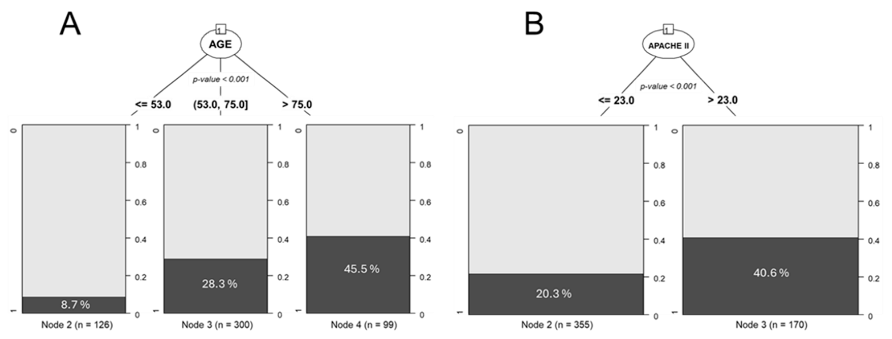
Figure 2.
CART-type AC model to establish the relationship between two variables. Values in bold indicate 28-day mortality. SGA: Subjective Global Assessment; BMI: Body mass index group. It is observed that the non-malnutrition group of obese patients has a lower mortality rate. R software (rpart library) was used [22].
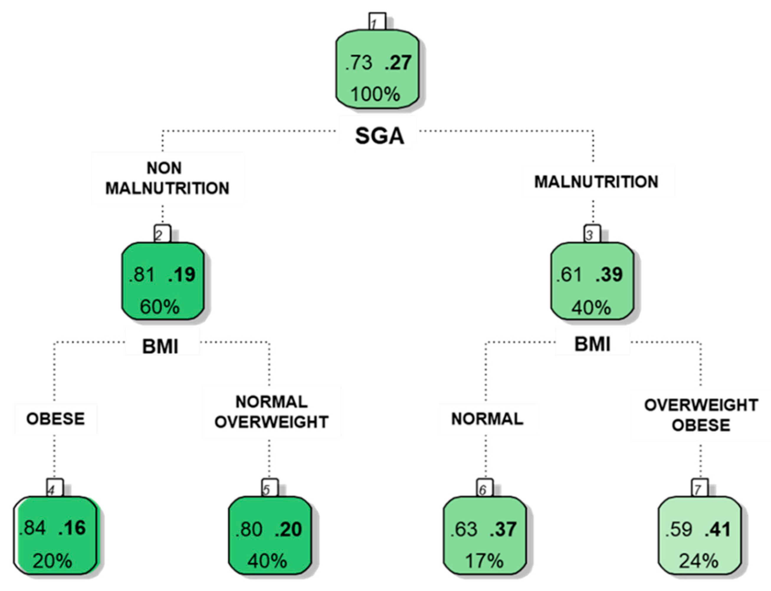
Figure 3.
Multivariate model based on CART-type. AGER: Age groups; SGA: Subjective Global Assessment; APA25: APACHE II score greater than 25; BMIG: Body mass index group; PROTEIN: Protein intake (g/kg/day). The hierarchy of variables is shown, and a special group in which obese patients have a lower mortality rate than those with overweight or a normal BMI is indicated in the red circle. Answer-Tree software used [19].
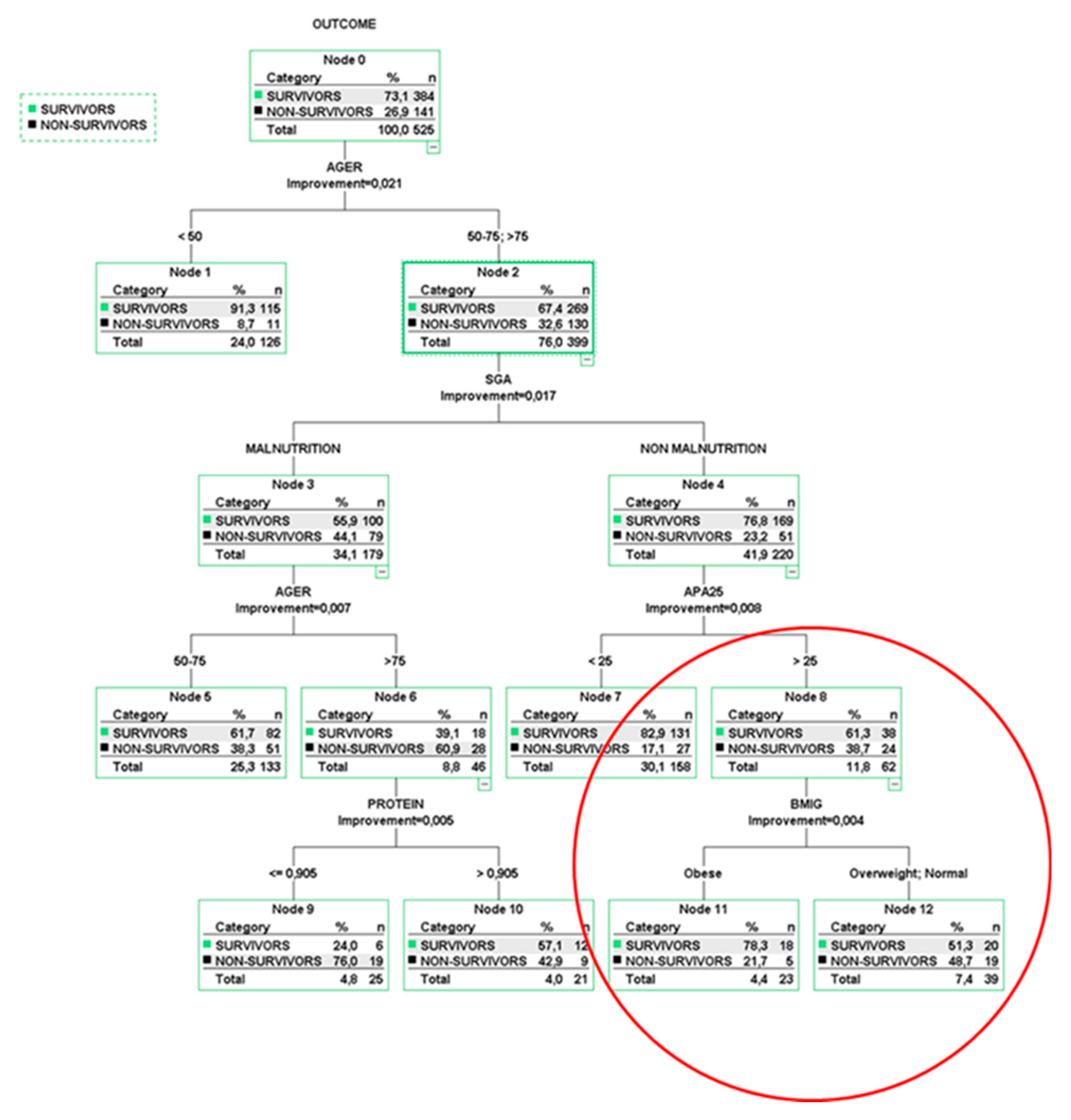
Figure 4.
Graph showing SHAP scores generated by the XGBoost model. AGER: Age groups; KCAL: Calorie intake (Kcal/kg/day); PROTEIN: Protein intake (g/kg/day); SGA: Subjective Global Assessment; APA25: APACHE II score greater than 25; BMIG: Body mass index group. The importance of each variable can be observed, with age being the greatest. It is also observed that the obese patient group has a negative impact on mortality, suggesting a paradoxical effect of obesity. R software (xgboost and SHAPforxgboost libraries) was used [22].
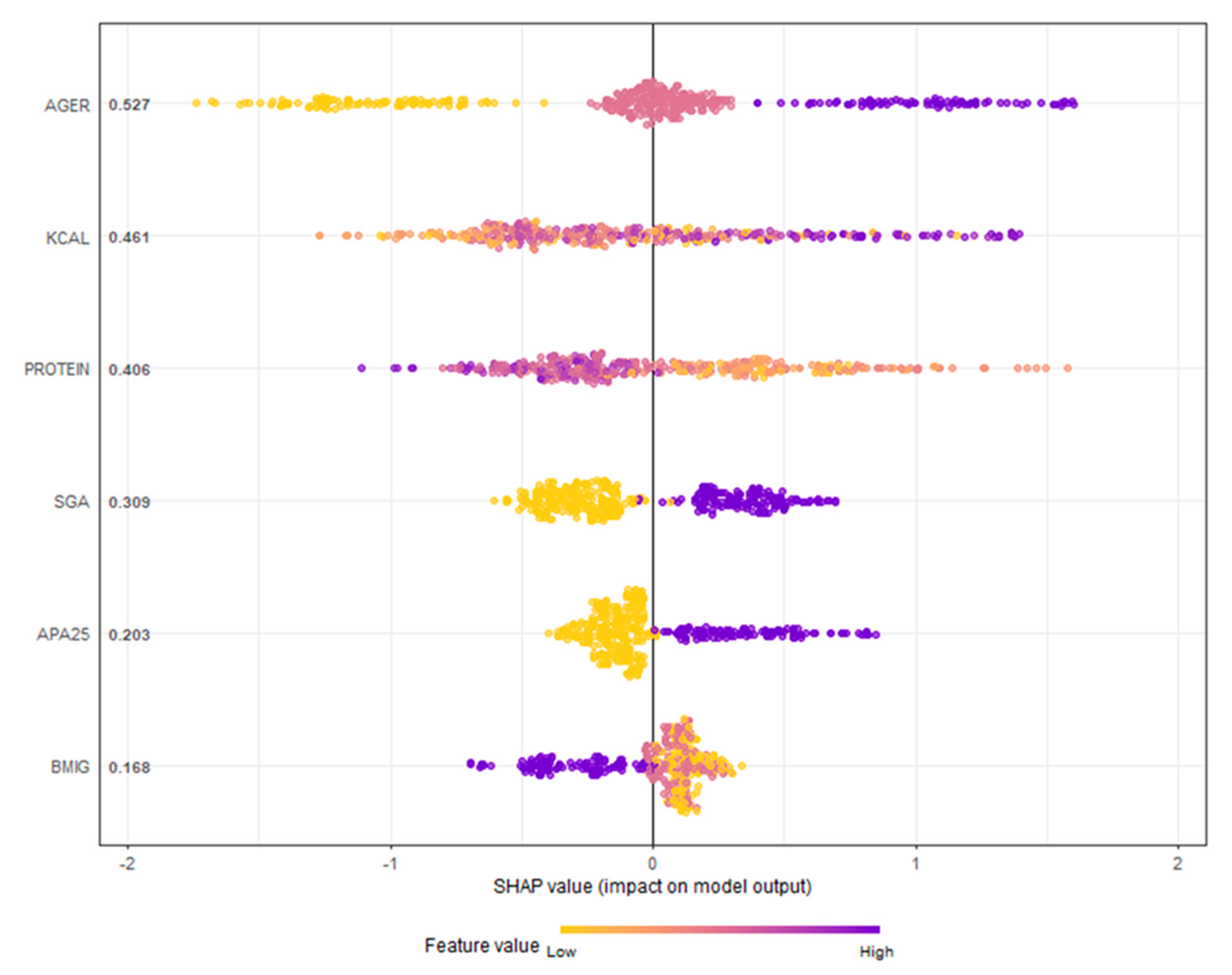
Figure 5.
Partial dependency graphs between each variable and mortality. AGER: Age groups; KCAL: Calorie intake (kcal/kg/day); PROTEIN: Protein intake (g/kg/day); SGA: Subjective Global Assessment; APA25: APACHE II score greater than 25; BMIG: Body mass index groups. We observed different behaviours between calorie and protein intake. Within the BMI groups, mortality was lower in the obese group. R software (SHAPforxgboost library) was used [22].
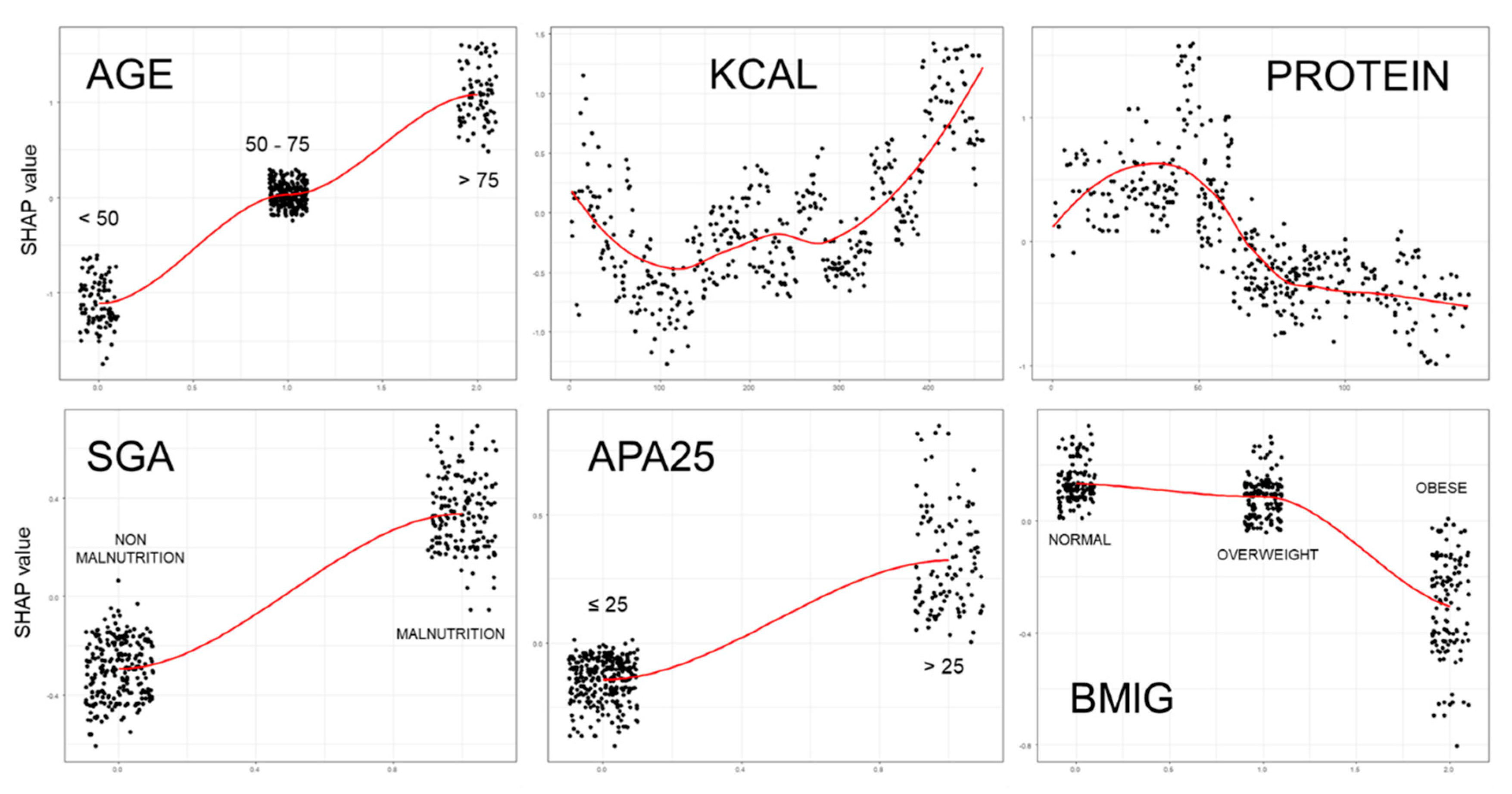
Figure 6.
ROC analysis of the developed models. The area under the ROC curve values are shown. LR: Logistic regression model; CART: CART-type classification tree; XGBoost: XGBoost-type ensemble classification tree model; Prob: Probability of death at 28 days. The LR and CART-type AC models had similar AUCs. The XGBoost model achieved better discrimination (Long's test with p < 0.001).
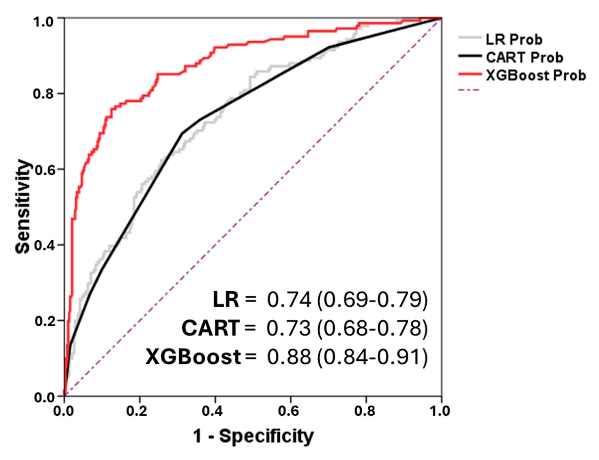

Table 1.
Types of classification trees.
| 1- SIMPLE CLASSIFICATION TREES | ||||
|---|---|---|---|---|
| CART | CHAID | C4.5 | ctree | |
| Description | Classification and Regression Tree | Chi-Square Automatic Interaction Detection | Concept Learning Systems Version 4.5 |
Conditional inference trees |
| Developer | Breiman (1984) | Kass (1980) | Quinlan (1993) | Hothorm (2006) |
| Primary Use | Many disciplines with little data | Applied statisticians | Data miners | Applied statisticians |
| Splitting Method | Entropy Gini index |
Chi-square tests F test |
Gain Ratio | Asymptotic approximations |
| Branch Limitations | Best binary split | Number of values of the input | Best binary split | Bonferroni-adjusted p-values |
| Pruning | Cross-validation | Best binary split p-value |
Misclassification rates | No pruning |
| Software * | Answer-Tree WEKA R - Python |
Answer-Tree R- Python |
WEKA R-Python |
R - Python |
| 2- ENSEMBLED CLASSIFICATION TREES | ||||
| Random Forest | AdaBoost | XG-Boost | ||
| Description | Uncorrelated forest | Adaptive Boosting | Extreme gradient boosting | |
| Developer | Breiman and Cutler (2001) | Freund and Schapire (1995) | Chen y Guestrin (2016) | |
| Ensembled Method | Bagging Parallel |
Adaptive Boosting |
Boosting Gradient Descent |
|
| Software * | R- Python-Java | R – Python - Java | R-Python - Java | |
| 3- HYBRID MODELS | ||||
| Fuzzy Random Forest | Random Forest Neural Network | |||
| Other method | Fuzzy logic | Neural Network | ||
| Developer | Olaru (2003) | Khozeimeh (2022) | ||
| Software * | C language | Python | ||
Table 2.
General characteristics, nutritional therapy, and outcomes of patients admitted to the ICU based on body mass index subgroup. Results of the ENPIC study [23].
Table 2.
General characteristics, nutritional therapy, and outcomes of patients admitted to the ICU based on body mass index subgroup. Results of the ENPIC study [23].
| All patients n = 525 |
Normal n = 165 |
Overweight n = 210 |
Obese n = 150 |
p-Value | ||
| Baseline characteristics & comorbidities | ||||||
| Age, years, mean ± SD | 61.5 ± 15 | 58.8 ± 16.5 | 62.8 ± 14.7 | 62.7 ± 13.5 | 0.05 | |
| Sex, male patients, n (%) | 67.2% (353) | 64.8% (107) | 74.8% (157) | 59.3% (89) | 0.003B | |
| Hypertension, n (%) | 43.6% (229) | 33.9% (56) | 41.9% (88) | 56.7% (85) | 0.01A, B | |
| Diabetes mellitus, n (%) | 25% (131) | 21.2% (35) | 20% (42) | 36% (54) | 0.001A, B | |
| AMI, n (%) | 14.1% (74) | 8.5% (14) | 16.7% (35) | 16.7% (25) | 0.04 B | |
| Neoplasia, n (%) | 20.6% (108) | 24.2% (40) | 19.5% (41) | 18% (27) | 0.11 | |
| Type of patient | Medical, n (%) | 63.8% (335) | 65.5% (108) | 62.9% (132) | 63.3% (95) | 0.81 |
| Trauma, n (%) | 12.6% (66) | 10.9% (18) | 15.2% (32) | 10.7% (16) | 0.75 | |
| Surgery, n (%) | 23.6% (124) | 23.6% (39) | 21.9% (46) | 26% (39) | 0.67 | |
| Prognosis ICU scores & nutrition status on ICU admission | ||||||
| APACHE II, mean ± SD | 20.3 ± 7.9 | 19.7 ± 7.6 | 20.1 ± 7.5 | 21.2 ± 8.5 | 0.18 | |
| Malnutrition (based on SGA), n (%) | 41% (215) | 52.7% (87) | 37.1% (78) | 33.3% (50) | 0.01 B | |
| Characteristics of Medical Nutrition Therapy | ||||||
| Early nutrition, < 48 h, n (%) | 74.9% (393) | 77.6% (128) | 75.2% (158) | 71.3% (107) | 0.43 | |
| Kcal/kg/day, mean ± SD | 19 ± 5.6 | 23.1 ± 6 | 18.6 ± 3.7 | 15.27 ± 4.24 | 0.001 A | |
| Protein, g/kg/day, mean ± SD | 1 ± 0.4 | 1.2 ± 0.4 | 1 ± 0.3 | 0.8 ± 0.2 | 0.01 A, B | |
| EN | 63.2% (332) | 59.4% (98) | 64.3% (135) | 66% (99) | 0.34 | |
| PN | 15.4% (81) | 13.3% (22) | 16.2% (34) | 16.7% (25) | 0.85 | |
| EN-PN | 7.8% (41) | 8.5% (14) | 7.6% (16) | 7.3% (11) | 0.92 | |
| PN-EN | 13.5% (71) | 18.8% (31) | 11.9% (25) | 10% (15) | 0.27 | |
| Outcomes | ||||||
| Mechanical ventilation, n (%) | 92.8% (487) | 89.1% (147) | 93.8% (197) | 95.3% (143) | 0.08 | |
| Vasoactive drug support, n (%) | 77% (404) | 73.9% (122) | 79.5% (167) | 76.7% (115) | 0.44 | |
| Renal replacement therapy, n (%) | 16.6% (87) | 16.4% (27) | 12.9% (27) | 22% (33) | 0.07 | |
| ICU stay, days, mean ± SD | 20.3 ± 18 | 18.2 ± 13.8 | 21.1 ± 17.1 | 21.6 ± 22.5 | 0.08 | |
| 28-day mortality, n (%) | 26.7% (140) | 29.1% (48) | 27.1% (57) | 23.3% (35) | 0.51 | |
AMI: Acute myocardial infarction; PN: Parenteral Nutrition; EN: Enteral Nutrition; SD: standard deviation; APACHE II: Acute Physiology and Chronic Health Disease Classification System II; SGA: Subjective Global Assessment; ICU: Intensive Care Unit. Statistically significant p-values are written in bold. Statistical results correspond to ANOVA p values. Bonferroni post hoc testing with statistically significant differences: A between Normal weight and obese subgroup; B between overweight and obese subgroup.
Table 3.
Multiple logistic regression model (LR) with 28-day mortality as the outcome variable.
| Variable | OR (95%CI) | p-value |
|---|---|---|
| Age (years) | ||
| < 50 | 1 | |
| 50-75 | 3.3 (1.7-6.5) | 0.001 |
| > 75 | 7.0 (3.3-14.9) | < 0.001 |
| SEX (MALE) | 1.0 (0.6-1.6) | 0.998 |
| APACHE II score | ||
| ≤ 25 | 1 | |
| > 25 | 2.2 (1.4-3.5) | < 0.001 |
| BMI groups | ||
| Normal | 1 | |
| Overweight | 0.9 (0.5-1.5) | 0.623 |
| Obese | 0.7 (0.4-1.4) | 0.651 |
| SGA | ||
| Non malnutrition | 1 | |
| Malnutrition | 2.6 (1.74.0) | < 0.001 |
| Median Kcal/Kg/day | 1.1 (0.9-1.1) | 0.315 |
| Median g protein/Kg/day | 0.3 (0.1-0.9) | 0.022 |
OR: Odds Ratio; CI: Confidence interval; APACHE II: Acute Physiology and Chronic Health Disease Classification System II; BMI: Body mass index; SGA: Subjective Global Assessment.
Disclaimer/Publisher’s Note: The statements, opinions and data contained in all publications are solely those of the individual author(s) and contributor(s) and not of MDPI and/or the editor(s). MDPI and/or the editor(s) disclaim responsibility for any injury to people or property resulting from any ideas, methods, instructions or products referred to in the content. |
© 2025 by the authors. Licensee MDPI, Basel, Switzerland. This article is an open access article distributed under the terms and conditions of the Creative Commons Attribution (CC BY) license (http://creativecommons.org/licenses/by/4.0/).
Copyright: This open access article is published under a Creative Commons CC BY 4.0 license, which permit the free download, distribution, and reuse, provided that the author and preprint are cited in any reuse.


