Submitted:
05 May 2025
Posted:
06 May 2025
You are already at the latest version
Abstract
For carbon peak by 2030 and carbon neutrality by 2060, China needs to balance efficiency and fairness to build a sustainable assessment system. The paper uses the Cobb-Douglas-Negative Feedback Model, finds that the green GDP development level of thirty-one provinces, cities and regions in China satisfies Ziff's law. By constructing the Double-Helix Coupling Model under the Lotka-Volterra symbiosis mechanism, the ecological supply capacity is to positively promote the level of ecological welfare or the ability to transform the ecological welfare, if and only if the co-gain parameters of . Zhejiang, Jiangsu, Shandong, and Guangdong provinces continue to support high ecological welfare and high green GDP from 2016 to 2023. They are model provinces for sustainable development in China. The development model of ecological welfare is still path-dependent by predicting the level of ecological welfare in thirty-one provinces, cities, and regions in China in 2030 and 2060. The path-dependent form will hinder the sustainable development of ecological welfare.
Keywords:
green GDP
; Ecological Welfare
; Sustainability
; Cobb-Douglas-Negative Feedback Model
; Lotka-Volterra mechanism
Introduction
The United Nations initially proposed the concept of Green Gross Domestic Product (GGDP) in the Integrated System of Environmental and Economic Accounting (SEEA) in 1993, and in SEEA (2000), SEEA (2003) and SEEA (2012) have continuously improved and optimized the GGDP accounting methodology, 1and emphasized the supporting role of the green accounting system in the 2030 Agenda for Sustainable Development and COP29. Through the Carbon Border Adjustment Mechanism (CBAM), the EU has highlighted the importance of internalizing negative externalities from the environment. The United States has promoted the transformation of green GDP from theory to practice through environmental industry classification and governance, input-output accounting, etc. France calls for a 40% reduction in emissions through a multi-year energy plan, and its National Low Carbon Strategy lays out a carbon neutrality pathway by 2050. Through its Clean Growth Strategy, the UK plans to invest £12 billion to support the green industrial revolution, create 250,000 jobs, and promote the development of offshore wind and hydrogen industries2. China will strive to peak carbon emissions by 2030 and achieve carbon neutrality by 2060. By the end of 2020, the output value of China's energy conservation and environmental protection industry was about 7.5 trillion yuan. 3The China Sustainable Development Assessment Report (2024) clarifies the practical path of linking green GDP accounting with regional coordinated development. Tianjin promotes the green transformation of coal-fired electronic units; Jiangsu to build a zero-carbon factory and carbon footprint service platform; Zhejiang deepens the construction of a collaborative innovation zone for pollution reduction and carbon reduction; All of them reflect the new paradigm of ecological priority regional development. 4Beijing, Shanghai, Guangdong and other provinces and cities have promoted China's sustainable development composite index to grow by 46.8% for seven consecutive years by optimizing resource and environmental efficiency5. The Kubuqi Desert Wind, Solar, Thermal Storage Integrated Base Project in Inner Mongolia has achieved an annual carbon dioxide emission reduction of 16 million tons through "green electronic direct supply", showing the synergistic effect of green GDP and the transformation of traditional industries. 6In 2024, 86% of the new renewable energy electronic generation capacity will be added, and the installed capacity of grid-connected wind and solar electronic will exceed 1.4 billion kilowatts for the first time, fulfilling China's commitment at the Climate Ambition Summit six years ahead of schedule. In the 2025 local government work report, keywords such as "pollution prevention and control", "green transformation" and "carbon reduction and emission reduction" appear often. In 2025, the national voluntary greenhouse gas emission reduction trading market will be officially launched, and the national carbon emission trading will become more active, marking a major step forward in the field of green and low-carbon economy in China. 7From 2015 to 2024, the average Gini coefficient of China is 0.466, close to the international warning level of 0.500, and the average Engel coefficient of urban residents and rural residents is 28.78% and 31.96%, respectively. Due to the limited financial ability and insufficient funds for ecological compensation in the west region, the progress of ecological restoration is often slow8. From 1999 to 2017, the discharge of wastewater in the west region increased by 39.39%, and the comprehensive use rate of solid waste was 11% less than that of the whole country9. According to the 2021 China Environmental Statistical Yearbook, SO2 emissions in the west region accounted for 43.82% of the national total in 2021. The Gansu Provincial Forestry and Grassland Administration mentioned in the 2023 self-assessment report on the performance of forestry and grassland ecological protection and restoration funds that although the funds released in advance, there are still problems of inefficient use of funds10; Since 2024, about 20% of the forest and grassland areas in the west region have been fragmented due to multiple departments, resulting in fragmented funding and inefficiency, resulting in slow progress in ecological restoration11. As the world's second largest economy, under the strategic framework of achieving the goals of carbon peak by 2030 and carbon neutrality by 2060, China needs to balance efficiency and fairness to build a new assessment system that takes into account the sustainable growth of the regional economy and the healthy, balanced and sustainable development of the regional economy.
1. Literature Review
Talberth et al. believe that the three major controversies in green GDP accounting are: the lack of resource pricing standards leads to poor comparability of accounting results; incomplete uniformity in the method of allocating environmental costs across periods; The impact of differences in international statistical caliber on cross-country comparisons. At the technical level, the dynamic assessment of ecosystem service value and the modeling of nonlinear environmental effects are still frontier problems[1]. CJ Cleveland believes that green GDP needs to incorporate natural non-market value into the accounting system, covering three core elements: ecosystem service value, resource stock depletion, and environmental pollution cost[2]. In terms of specific accounting methods, Li and Fang and other scholars used the ecosystem service value method to calculate the ecological service value of land cover type through satellite remote sensing and GIS technology, and constructed a global green GDP map[3]; Sun, Jia and other scholars use the energy analysis method to separate the costs of water consumption and pollution damage from the traditional GDP, and use the resource and environmental loss adjustment method to emphasize the net the welfare assessment of economic output[4]; Nahman, Mahumani and Lange scholars tried to construct a green economy index covering key parameters such as carbon emission intensity and renewable energy proportion through the composite index method, so as to provide a quantitative basis for policy optimization[5]. Z Liu, D Guan and other scholars emphasized the concept that provincial carbon emission targets need to be designed in tandem with energy allocation and industrial transfer policies[6]. Nahman, Mahumani, and Lange also suggested the establishment of a green GDP-oriented fiscal transfer mechanism to ensure that ecological reserves are properly compensated[5].
Empirical analysis of panel data from 2012 to 2021 in 11 provinces in the Yangtze River Economic Belt found that there was a significant positive spatial correlation between industrial green GDP growth and ecological footprint, and there was inter-provincial heterogeneity in this association[4]. Y Yu and M Yu et al. used the CA-Markov model to predict the spatiotemporal evolution of China's green GDP from 2020 to 2050, and although the total green GDP will continue to grow in the future, the ecosystem service value (ESV) will decline due to the expansion of construction land, and regions such as the North China Plain and the Yangtze River Delta will face significant ecological deficits[7]. Li and Fang scholars constructed the world's first spatially explicit database of green GDP by integrating DMSP/OLS nighttime light data with Glob Cover land cover data[3]. Z Liu, D Guan and other scholars proposed regional differentiated emission reduction pathways[6]. Brajer, Mead, and Xiao found that first-tier cities such as Beijing and Shanghai have achieved an inflection point in pollutant emissions through technological innovation, but the central urban agglomeration is still in the EKC rising stage[8]. Scholar Wang emphasized that green GDP accounting needs to be linked to the audit system of natural resource assets[9]. Scholars Caviglia-Harris, Chambers, and Kahn argue that economic growth alone cannot automatically improve environmental quality, and that environmental tax reform is needed to link ecological compensation standards to green GDP[10].
Tang Shaoxiang et al. found that policies such as energy tax and environmental governance subsidies can effectively promote the coordinated development of the economy and the environment by constructing a green GDP social accounting matrix and using the CGE model for simulation analysis. At the same time, it emphasizes the importance of policy simulation in evaluating the effects of different policies, and points out that the CGE model can simulate the economic and environmental impacts under different policy scenarios, so as to provide a scientific basis for policy formulation[11]. Fang Shijiao and Xiao Quan found that there is a significant spatial spillover effect on ecological welfare performance through spatial measurement method, and the economic activities and policy impacts between regions are interrelated, and suggested that ecological welfare performance should be improved by strengthening inter-regional coordination and cooperation, optimizing energy structure and industrial structure, and improving the level of environmental regulation[12]. Dong et al.'s research further expanded the decomposition of the driving factors of ecological welfare performance, and found that economic efficiency and urbanization scale are the main factors to promote the improvement of ecological welfare performance, while population dispersion is the main constraint, and local governments should fully explore the driving factors affecting ecological welfare performance and formulate differentiated incentive policies to promote regional sustainable development[13]. Zang Mandan et al.'s research found that by optimizing the economic structure and improving the efficiency of resource utilization, developing countries may achieve economic growth while improving environmental quality[14].
Costanza believes that the essence of ecological welfare is the value realization of ecosystem service flow in the dimension of human welfare, and natural capital flows to the socio-economic system through four types of services: "supply-regulation-support-culture".[15]. The level of the welfare should be determined by the set of feasible capabilities actually enjoyed by the individual, and the ecological elements are the result of expanding the boundaries of feasible capabilities on the basis of the original feasible capacity set by ensuring a healthy environment and providing development resources. The dissipative structure is formed through nonlinear interaction between ecology and the welfare system, and there is also a threshold effect and co-evolution mechanism between the systems.
The construction of green GDP and the evaluation of ecological performance by scholars at home and abroad are diverse, and the establishment of each index makes up for and improves various problems met in environmental economic development. However, most scholars have proved indicators that are problematic. (1) The process of constructing indicators is too complicated. For example, Tang Shaoxiang et al. calculated the value of China's green GDP in 2007 by constructing a SAM table of green GDP[11]The process is scientific, rigorous and effective in theory, but it requires huge transaction costs in practice.(2) There is a lack of corresponding mathematical models as support. For example, Li and Fang used satellite remote sensing technology and GIS technology to map green GDP[3]In essence, it still adopts the model of "constructing indicators, selecting regression models, adjusting regression models, and explaining regression results", and the constructed green GDP indicators still rely on the results of empirical analysis and lack theoretical models as support. Dong Han and other scholars used the data from the World Bank and EPS official to reduce the dimensionality of the data through principal component analysis, and constructed an accounting method for green GDP according to the characteristics of principal components[13], which still has the problem of lack of theoretical models. And (3) the inability to effectively and concisely quantify green GDP. Most of the empirical models mentioned in the above paper rely on the characteristics of the data itself, and the empirical results will be different due to different data selection and processing methods. This discrepancy cannot be resolved by empirical evidence alone. Compared with the above-mentioned papers, the biggest innovation of the article is that::(1) Drawing on the logical growth model in biology, Negative feedback regulation mechanism and Lotka-Volterra symbiosis model, Combined with the Cobb-Douglas production function,The theoretical model of green GDP and the coupling model of ecological welfare double helix model constructed.(2) Using the CA-Markov model to predict 2030, In 2060, the GGDP and ecological welfare levels of thirty-one provinces, cities and regions in China will be comprehensively judged to be able to achieve sustainable development.
2. Model
2.1. Cobb-Douglas-Negative Feedback Model
2.1.1. Establishment of a Net Environmental Revenue (NER) Model
Zhang Tianming (2017) pointed out that pollution control costs (such as sewage treatment and garbage incineration) should be deducted to force source treatment and truly reflect the balance between economy and environment. Pro-deduction advocates generally believe that governance investment is the cost of the "pollution first, clean up later" model, which is essentially the internalization of negative externalities of economic activity, and should be deducted from GDP to reflect the real level of growth. Jie (2004) proposed that the investment in pollution control itself is part of economic activities, which will increase GDP, while the loss of environmental pollution will be used as a subtraction, and the two will not affect the traditional GDP growth rate after offsetting. According to the recommendations of the Integrated System of Environmental-Economic Accounting (SEEA) proposed by the World Bank and the United Nations Environment Programme (UNEP), pollution control investments are presented separately and are neither directly deducted nor fully retained, but are used as supplementary information to assess the environmental efficiency of economic activities.
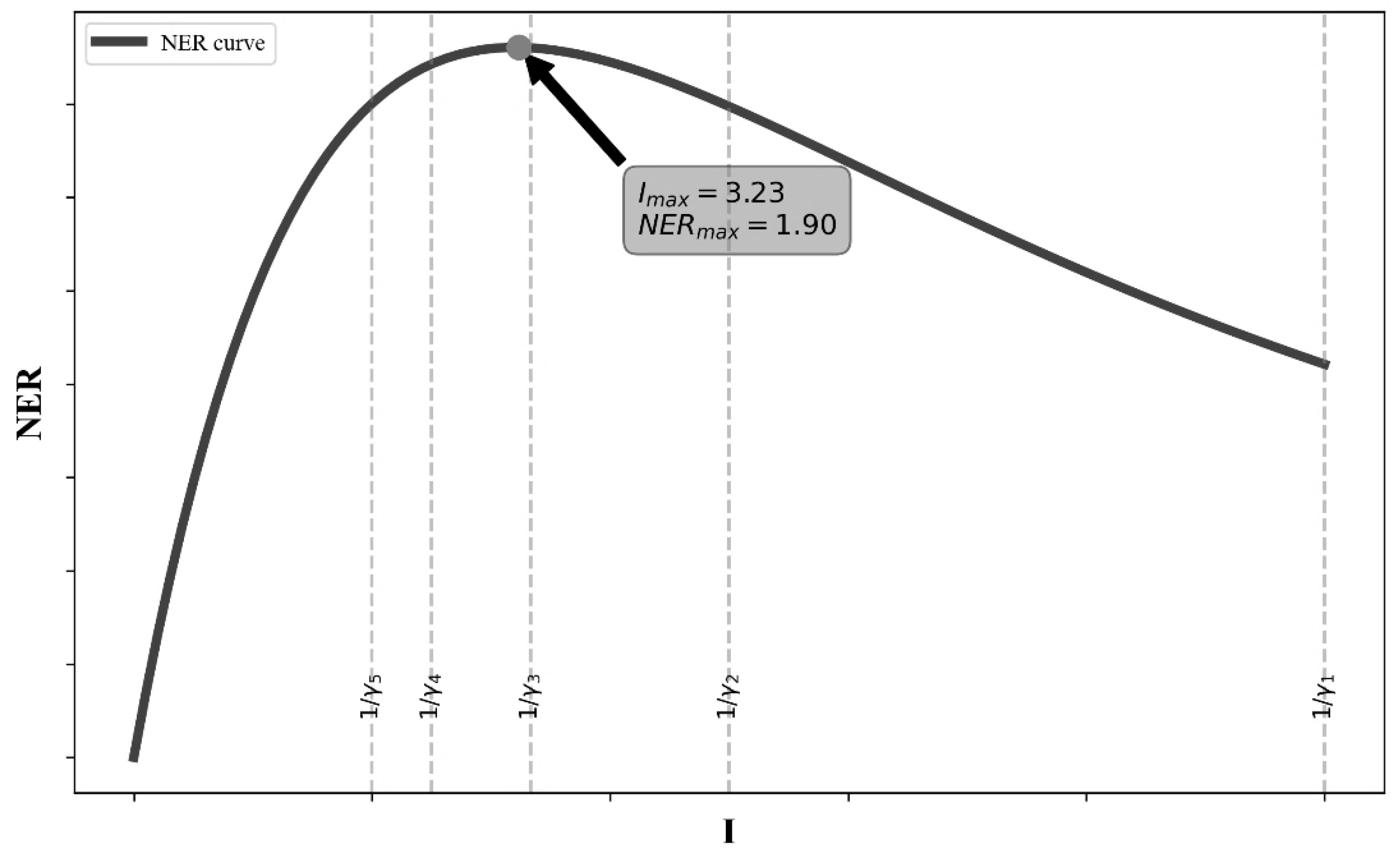
Figure 1.
where
According to the data provided by the National Bureau of Statistics, combined with the United Nations method of accounting for GGDP, the paper calculates NER through the production function of double externality marginal return:
- : the investment in the treatment of pollutants
- : the pollutants cost of
- : the coefficient of environmental returns per unit investment of pollutants
- : the deceleration rate of marginal returns of pollutants
- : the hazard coefficient of pollutant emissions
By equation (2). Get:
When , it means that with the increase in the scale of investment in environmental pollution control, the technical effect is greater than or equal to the impact of the internalization of negative externalities; When , it meant that when increase, the scale of investment in environmental pollution control decreased, and the technical effect was less than the impact of the internalization of negative externalities. The entire curve takes on an “inverted U-shape" shape (Fig.1). The critical value represents the critical value of the investment in pollutant treatment of , and when it is greater than the critical value, will decrease with the increase of investment in pollution control.
From equation (2), the paper can also get:
From equation (4), it can be seen that the impact on NER is negative, because the emission of pollutants always brings negative externalities to the environment.
GGDP is GDP that takes into account environmental costs, according to the initial definition of GGDP:
Among them, GGDP stands for Green GDP, GDP is GDP in the traditional sense, and NER is Net Environmental Revenue. However, the problem with the calculation method of equation (1) is that if the increase in GDP is greater than the decrease in NER, the increase in GGDP is driven by the increase in GDP, although the overall increase in GGDP increases. In the same way, if the increase in NER is less than the decrease in GDP, then the GGDP decreases overall, but the increase in NER means the strengthening of environmental governance and the increase in Net Environmental Revenues, and this effect should be reflected in the GGDP, but if it is only according to Eq. (5). It is not possible to present this law effectively and scientifically.
- Based on the shortcomings reflected in equation (5), the following accounting method will be used in the paper:It stands for thirty-one provinces and regions in China and is the year (2015-2023). Relative indicators such as growth rate () rather than absolute indicators are used to reflect the dynamic changes of the economy and the environment, and avoid the limitation of inconsistent dimensions of static indicators.
2.1.2. Establishment of Green GDP (GGDP) Model
Combined with equation (6), (7) and (8), the following results are obtained:
Satisfied :
- if and , then ;
- If and , then ;
- If and , then .
- Satisfied :
- if , then ;
- If , then ;
- If , then .
By giving different relatives to economic and environmental factors, policymakers can adjust according to the stage of development or regional characteristics:
- if , which means , then the elasticity to GGDP is greater than the elasticity to GGDP;
- if , which means , then the elasticity to GGDP is less than the elasticity to GGDP;
- if , which means , then the elasticity to GGDP is equal to the elasticity to GGDP.
From equation (9), it can be obtained:
The technological substitution rate to the obtained:
- if , which means , then the substitution ability of towards is exponentially efficient;
- if , which means , then the substitution ability of towards is decreasingly efficient;
- if , which means , then the substitution ability of and is equally efficient.
2.1.3. Establishment of Green GDP (GGDP) Growth Rate Model
- The formula for calculating the growth rate of GGDP before the correction is as follows:
- if , then ;
- if , then ;
- if , then .
- The formula for calculating the modified GGDP growth rate is:
2.2. The Double Helix Coupling Model (DHCM) Was Established
2.2.1. Establishment of Ecological Supply Capacity (E) Model
- Based on the integrated framework of ecosystem service theory and welfare economics, the paper will construct a Dual Helix Coupling Model (DHCM) to provide theoretical support for the estimation of ecological welfare.
- The ecological supply function is defined as follows:
- the core element of the ecological subsystem
- the element elasticity coefficient
- the correction factor of regional ecological carrying ability
- the weight of the abilities.
For E with respect to the partial derivative of , the paper gets:
Since , all other things being equal:
- If , then , The marginal revenue of E is increasing;
- If , then , The marginal revenue of E is decreasing;
- If , then , The marginal revenue of E is constant.
2.2.2. Establishment of the Welfare Conversion Capacity (W) Model
- Benefit conversion functionsatisfy:
- the possible ability component ().
- the weight of the abilities ().
- marginal transformation efficiency ().
- the system quality adjustment coefficient ().
For with respect to the partial derivative of , the paper get:
- If , then , The marginal revenue of W is increasing;
- If , then , The marginal revenue of W is decreasing;
- If , then , The marginal revenue of W is constant.
2.2.3. Establishment of the Ecological Welfare-Being (EWI) Model
The ecological welfare index is the coupling output of the ecological supply function and the welfare transformation function, and the relevant content of the improved Lotka-Volterra symbiosis model in biology can be obtained
- the ecological self-organization coefficient;
- the welfare self-organization coefficient ;
- the co-gain parameter
- the critical value of ecosystem collapse
- the critical value of social the welfare economic system collapse.
- The hyperbolic tangent function is used to characterize the nonlinear interaction between systems.
2.2.4. The Welfare Analysis
- From equation (26), it can be seen that:
From Eq. (26), the following results can also be obtained:
Thereinto:
Eq. (30) shows that ecological supply capacity and the welfare transformation level have an interactive effect on ecological welfare. Equations (27) and (28) also give the following results:
The definition of are given in equations (31) and (33).
- When :
- If satisfied
- If satisfied
- If satisfied
When:
- If satisfied
- If satisfied
- If satisfied
3. Empirical Analyses12
3.1. The Experience of the Cobb-Douglas-Negative Feedback Model
3.1.1. Empirical Evidence of Net Environmental Revenues (NER) Results
Combined with the specific development of China and the National Bureau of Statistics, the NER indicator is constructed as shown in equation (27).
According to the model constructed from equations (1) to (19) and (41), combined with the GDP and NER data of 31 provinces, cities and regions in China, the number of samples conforming to the GGDP theoretical model accounted for 92.17% of the total number of samples through empirical analysis (Fig. 2). The theoretical model has high empirical significance.

Table 1.
NER and GDP indicators are established.
| Level 1 indicators | Secondary indicators | Meaning | Data source |
| NER | Investment in industrial waste gas treatment | NBSC | |
| Investment in industrial wastewater treatment | NBSC | ||
| Investment in industrial waste treatment | NBSC | ||
| Investment in industrial noise control | NBSC | ||
| Other governance investments | NBSC | ||
| Nitrogen oxide emissions | NBSC | ||
| Sulphur dioxide emissions | NBSC | ||
| Particulate matter emissions | NBSC | ||
| GDP | GDP | Gross regional product | NBSC |
3.1.2. Empirical Results of the Green GDP (GGDP) Growth Rate Model
NER satisfies Ziff's law (Fig. 3, Tbl.2), which indicates that the distribution of NER among 31 provinces and regions in China is uneven, and in order to make GGDP more affected by NER than GDP, it is necessary to reconstruct the accounting index of GGDP to reflect the "inverted U-shaped" impact of NER on GGDP ".
According to equations (14) to (17), combined with the data of NER, GDP and GGDP of 31 provinces, cities and regions in China, the growth rates of GGDP, GDP and NER are obtained, and it is found that the growth rate of GGDP is between the GDP growth rate and the NER growth rate, and when the growth rate of NER is greater than the growth rate of GDP, the growth rate of GGDP is greater than the GDP growth rate. Vice versa. The correctness of this conclusion is verified by empirical results.
From the perspective of provinces and regions, it is found that the NER growth rate among the 31 provinces, cities and regions in China has a large fluctuation, and the frequency of peaks and troughs is high, indicating that the level of environmental governance investment among the 31 provinces, cities and regions is uneven. From the perspective of time, the change of NER growth rate is not stable, indicating that the level of control of environmental governance investment in China's 31 provinces, cities and regions is different, and the provinces, cities and regions with a sudden large increase and a large decrease in the NER growth rate need to be paid attention to, if the scale of environmental governance investment exceeds the optimal point, it will prevent the NER from continuing to rise, and if it exceeds the optimal point too much, it will lead to a sharp decline in NER, resulting in a negative growth rate of NER (Fig.4).
In general, the changes in the growth rates of GGDP, GDP and NER are in line with the model, and in the chapter "Robustness Analysis", the article will detail the changes of this negative feedback adjustment law when different parameter values are taken.
3.1.3. Empirical Results of the Green GDP (GGDP) Model
In 2023, the GGDP of Jiangsu Province is 2.2659, and the growth rate is 12.96%, indicating that the synergy between economic growth and ecological environmental protection in Jiangsu Province in 2023 is strong. The growth rate of GGDP in Zhejiang Province is 23.69%, and the growth rate of Net Environmental Income (NER) is 50.05%, indicating that most of the growth of GGDP in Zhejiang Province is driven by the improvement of environmental benefits. The growth rate of GGDP in Shanghai and Anhui Province was -10.55% and -14.81%, respectively, and the NER growth rate in Anhui Province was -29.54%, showing that it faces challenges in balancing economic growth and environmental sustainability (Tbl.3).
In 2023, Shanghai's development model will be "high-quality synergy", with outstanding levels of GGDP and NER, reflecting the technological effects brought about by green governance investment. Jiangsu Province's development model in 2023 is "scale-oriented", with the GGDP level ranking first in the Yangtze River Delta region and the NER at a medium and low level, partly due to the technological effects brought about by green governance investment, and partly the result of the internalization of negative externalities in order to control environmental pollution. Zhejiang Province is "balanced development", and the levels of GGDP and NER are at the upper middle level. Compared with Jiangsu, Zhejiang and Shanghai, Anhui Province is a "potential catch-up type", and the GGDP and NER values are at a medium and low level, so it is necessary to avoid a path-dependent economic development model.
In 2023, the development of GGDP in the Beijing-Tianjin-Hebei region will show a clear differentiation trend. Beijing's GGDP is 1.3269, with a growth rate of 8.47%, which is the most outstanding performance in the region, indicating that its economic green transformation has achieved remarkable results. Tianjin's GGDP is 1.1268, with a growth rate of -3.44%; Hebei Province has a GGDP of 1.4087, but a growth rate of -26.24%, showing that its green economy is facing serious challenges. This regional disparity reflects the uneven development of the Beijing-Tianjin-Hebei region (Tbl.4).
Beijing's NER is 1.1910, which is smaller than Tianjin's 2.0000, but Beijing's GGDP is 1.3269, which is greater than Tianjin's 1.1268, indicating that although Beijing's NER rises due to the influence of technological effects, the negative externality internalization has a negative impact on Beijing's NER that decreases, so that Beijing's NER is less than Tianjin's. The GGDP of Hebei Province is the highest in the Beijing-Tianjin-Hebei urban agglomeration, but its NER is the least, and the negative impact of negative externality internalization on NER is higher than the positive effect of technology effect on NER, resulting in the NER being at the least level.
In 2023, there will be a clear polarization within the Chengdu-Chongqing urban agglomeration. Sichuan Province's GGDP reached 1.6046, with a growth rate of 3.74%, while Chongqing's GGDP was 1.3122, with a sharp decline of 31.21%, showing a serious recession. This difference is mainly due to the contrast between the performance of the two places: the NER of Sichuan Province increased by 1.36%, while the NER of Chongqing City plummeted by 52.80%, but the GDP growth rate of both places remained above 5%, indicating that the traditional economic growth has not been significantly affected, but the effect of green transformation is significantly different (Tbl.5).
The GGDP of Sichuan Province is greater than that of Chongqing Municipality, but the NER of Sichuan Province is 1.1786, which is smaller than that of Chongqing NER of 1.2939, indicating that the impact of the internalization of negative externalities in the process of investment in environmental pollution in Sichuan Province in 2023 is greater than the impact of technological progress. This leads to a drop in NER.
In 2023, the three provinces in the urban agglomeration in the middle reaches of the Yangtze River will all show a negative growth trend of GGDP, of which Jiangxi Province will decrease by -32.95%, Hubei Province will be -23.32%, and Hunan Province will be -13.96%. Jiangxi, Hubei and Hunan provinces all maintained positive GDP growth of 3.16%, 5.81% and 5.16% respectively, but NER all fell sharply, with -48.82% and -42.53% respectively -27.84%, which indicates that there is a clear imbalance between economic growth and environmental protection in the region in 2023. Jiangxi Province had the lowest GDP growth rate (3.16%), but the NER decreased the most (-48.82%), reflecting that its economic development mode is still relatively extensive and the environmental costs are high (Tbl.6).
Hunan Province has a high level of GGDP and NER, with a NER of 1.2138, which is the highest, and a GGDP of 1.4800, indicating that the technological effects of environmental governance investment in Hunan Province in 2023 are greater than the impact of negative externalities internalization.
There are significant differences in the green economic development of the three provinces and regions of the Beibu Gulf urban agglomeration. Guangdong Province performed the most prominently, with a GGDP of 2.2809 and a growth rate of 4.35%, with positive GDP and NER growth. The growth rate of GGDP in Guangxi and Hainan was negative, -33.61% and -41.22% respectively, and the NER growth rate in Hainan was even less at -74.09%, showing that these two regions have paid a large environmental price in economic development. Although Hainan Province's GDP growth rate is as high as 9.60%, its environmental indicators are at a low level, reflecting the obvious unsustainability of its economic growth model (Tbl.7).
Guangdong Province is at the highest level for both GGDP and NER. The results show that the technological effect of investment in environmental pollution control is greater than the impact of negative externality internalization.
The correlation coefficient between GGDP and NER changed from 0.894 to 0.983 during the rapid improvement period from 2016 to 2018, reflecting the marginal improvement effect brought about by the strengthening of environmental protection policies in the early stage of the 13th Five-Year Plan. During the high and stable period from 2018 to 2021, the correlation coefficient remained in the range of 0.93-0.98, showing that the green development model tends to mature. During the slight correction period from 2022 to 2023, its correlation coefficient fell to the range of 0.90-0.95 due to the impact of the epidemic, but it still supported a strong correlation. In 2023, the correlation coefficient will rise to 0.949, reflecting the effect of the implementation of the "dual carbon" policy and economic policies in the post-epidemic era. In summary, China's economic development model has achieved a fundamental shift from "environmental cost" to "environmental friendliness", and this transformation is sustainable and resilient (Fig.5).
From Fig.6, Tbl.8 shows that through (6), the green GDP values of 31 provinces, cities and regions meet Ziff's law, showing that the development of China's green GDP is unbalanced. Due to the advantages of technology, capital and policy, developed regions can achieve local green transformation faster and drive the development of less developed regions; Underdeveloped regions are unable to develop on their own due to lack of resources.
Jiangsu, Zhejiang, and Shanghai are home to about 20% of the country's high-tech industries13, and the proportion of traditional high-polluting industries in the central and west regions is currently about 30%-40%, and it is on the rise14. This development trend of driving the more backward central and west regions through the "growth pole" - the eastern region is one of the fundamental reasons for the distribution of green GDP to satisfy Ziff's law.
3.1.4. Sustainability Index (SI) Measurement
Sustainable economic development in environmental economics is defined as development that meets the needs of current economic development without producing negative externalities caused by environmental pollution as much as possible. The Sustainability Index (SI) is defined in the following way:
3.1.5. CA-Maekov Predicts the Results of the Sustainability Index (SI)
To predict the sustainable development index (SI) of 31 provinces, cities and regions in China from 2024 to 2050, the paper uses the CA Markov model to make the prediction. From 2015 to 2023, the sustainable development index (SI) levels of 31 provinces, municipalities, and regions in China (Fig.7) are divided into three types, and the specific classification results are shown in Tbl.9:
According to the China Sustainable Development Assessment Report 2023, the average annual growth rate of the low-carbon development index of China's eastern coastal provinces is 1.7 times that of the west resource-based provinces. The probability that provinces and regions that will maintain a high level of sustainable development in 2023 will still maintain this level in 2060 is 84.04% (Tbl.9), indicating that the path dependence and institutional resilience of sustainable development capacity are essentially the result of the three-way coupling of "system-technology-capital". The sustainable development model of some provinces and cities in China has advanced from the "exploration stage" to the "mature replication stage" (Tbl.10).
Table 10.
SI levels predicted by CA Markov model ().
| SI level | In 2030 | Year 2060 |
|---|---|---|
| Elevated level of status | Xinjiang Uygur Autonomous Region, Qinghai, Heilongjiang, Liaoning, Beijing City, Shanxi, Shaanxi, Chongqing Municipality, Henan, Shandong, Anhui, Jiangsu, Zhejiang, Fujian, Guangdong, Guangxi Zhuang Autonomous Region, Hainan | Xinjiang Uygur Autonomous Region, Qinghai, Yunnan, Guangxi Zhuang Autonomous Region, Guangdong, Hainan, Hunan, Chongqing Municipality, Fujian, Zhejiang, Jiangsu, Anhui, Henan, Hebei, Liaoning, Jilin, Heilongjiang |
| Moderate level of status | Tibet Autonomous Region, Sichuan, Gansu, Ningxia Hui Autonomous Region, Guizhou, Jiangxi, Hebei, Jilin | Sichuan, Hubei. Shanxi, Ningxia Hui Autonomous Region |
| Low-level state | Inner Mongolia Autonomous Region, Hubei, Hunan, Yunnan | Tibet Autonomous Region, Inner Mongolia Autonomous Region, Gansu, Shaanxi, Shandong, Jiangxi, Guizhou |
Table 11.
SI transfer matrix from 2023 to 2030/2060 ().
| SI | 2030/2060 | |||
|---|---|---|---|---|
| 0 | 1 | 2 | ||
| In 2023 | 0 | 0.4516 | 0.1935 | 0.3549 |
| 1 | 0.3448 | 0.4828 | 0.1724 | |
| 2 | 0.0745 | 0.0851 | 0.8404 | |
Sustainable development has the characteristics of strong inertia, which is embodied in the formation of systematic investment in green energy, scientific and technological innovation, ecological protection, and other fields. The cumulative effect of these infrastructure and policy frameworks will continue to drive low-carbon development for decades to come. For example, in regions such as Zhejiang and Qinghai, the current layout of renewable energy and ecological compensation mechanisms has the characteristics of long-term returns.
The resilience of the governance system is reflected in the government's strong planning execution and adaptive governance capabilities, which can withstand external shocks. In contrast, some regions that rely on traditional energy sources may experience greater volatility in their sustainability levels if they do not make the transition in time.
This kind of inertia and resilience will promote the development of the regional economy on the one hand, but on the other hand, it will lead to the Matthew effect. According to the Myrdal's theory of cumulative cyclic causality, regional development is accompanied by an echo effect in addition to the concomitant diffusion effect. At present, the leading regions form a positive cycle through the accumulation of technology, capital, and talents, while the backward regions have become more difficult to catch up.
3.2. Experience of the Double Helix Coupling Model (DHCM)
3.2.1. Empirical Results of the Ecological Welfare (EWI) Model
The "coupled index system" was adopted for the calculation of ecological welfare in thirty-one provinces and cities in China, and the two-dimensional evaluation of "ecology and welfare" was realized through the combination of ecological supply capacity and the welfare transformation efficiency. Here is how to build metrics.
Table 12.
Establishment of ecological welfare indicators.
| Dimension | Level 1 indicators | Secondary indicators | Data source |
|---|---|---|---|
| Ecological supply capacity (E) | Resource supply capacity | Total amount of water resources | Water Resources Bulletin |
| Forest cover | Nbs | ||
| Environmental quality level | PM2.5 concentration | China Statistical Yearbook | |
| Proportion of surface water | Water Resources Bulletin | ||
| Ecological regulation capacity | Arable land | International Bureau of Statistics | |
| Carbon emissions | China Carbon Accounting Database | ||
| Level of The welfare Conversion (W) | Basic Coverage | Natural population growth rate | NBSC |
| Number of beds in medical institutions | NBSC | ||
| Development opportunities | Number of undergraduate graduates | NBSC | |
| Expenditure on scientific research | NBSC | ||
| Distributive fairness | Gini coefficient | NBSC | |
| Urban-rural income ratio | NBSC |
Combining the values of GGDP and EWI, the 31 provinces, cities and regions in China are divided into four types: "high GGDP, high EWI", "low GGDP, high EWI", "low GGDP, low EWI", and "high GGDP, low EWI". Zhejiang, Jiangsu, Shandong, and Guangdong provinces are all in the "high GGDP, high EWI" quadrant from 2019 to 2023, indicating that the green GDP development level of these four provinces continues to be high, and the ecological welfare is maintained at a high level, which not only achieves sustainable regional economic growth, but also achieves sustainable regional economic health and development. In 2019 and 2021, Shanghai was at the level of "high GGDP, low EWI", and although it can achieve sustainable economic growth, its ecological welfare is at a low level. The ecological (E) and the welfare (W) values of Zhejiang, Shandong, and Guangdong provinces are all within the quadrant of "high ecology (E) and high the welfare (W)", showing that their ecological level and the welfare level at an elevated level. The welfare (W) of Jiangsu Province is at an elevated level, but the ecology (E) is at a low level, showing that Jiangsu Province needs to strengthen the protection of the ecological environment and avoid excessive investment in environmental pollution control. Shanghai's ecology (E) and the welfare (W) are both at low levels, resulting in a low level of EWI (Fig.8).
Most provinces, cities and regions are in a "low GGDP, high EWI". The quadrant shows that most of China's provinces, cities and regions do not fully balance economic growth with environmental protection and governance, and excessive environmental pollution leads to an increase in investment in environmental pollution control, which can be seen from the analysis of equations (2) to (8), which will inhibit the rise of NER and then affect the growth of GGDP. The high level of EWI is mainly since the investment in environmental pollution control itself will indirectly restore the resource supply ability, environmental quality level and ecological regulation ability, and then make the ecological welfare fluctuate smoothly. The vast majority of provinces, cities and regions are at a high level of the welfare (W) (Fig.9), but there is still an imbalance in the development of the environment (E), so China's 31 provinces, cities and regions should not only continue to pay attention to investment in environmental pollution control, but also pay more attention to the protection of the natural environment itself.
Under the premise of maintaining sustainable development, China's 31 provinces, cities and regions need to maintain the investment in environmental pollution control within an appropriate range as much as possible, and a certain scale of investment in environmental pollution control reflects the development of green investment and green technology, but too much investment will lead to the internalization effect of negative externalities greater than the scale effect of technology, resulting in a decrease in NER, which in turn leads to a decline in GGDP. In order to solve this problem, the first is to improve the technical level and obtain the best governance effect with the least amount of money; The second is to reduce environmental pollution, from the very beginning to pay attention to the protection of the environment, in order to reduce the scale of investment in environmental pollution control.
3.2.2. CA-Maekov Predicts the Results of Ecological Welfare-Being (EWI)
Combined with Tbl.13 and the transfer matrix in Tbl.14, the EWI level in most provinces, cities and regions still has a high probability of remaining in the original state. The results show that the level of regional ecological welfare will solidify in the future, in which the probability of maintaining a low level of EWI is 95%, the probability of maintaining a medium level of EWI is 80.95%, the probability of maintaining a high level of EWI is 88.10%, the probability of EWI being a low level of EWI jumping to a high level in the future is almost 0, and the probability of EWI being a medium level of jumping to a high level of state in the future is only 4.76%. These phenomena fully reflect the dilemma of ecological welfare development today, and reflect that there is an obvious hierarchy in the development level of ecological welfare in 31 provinces, cities and regions in China, and the path dependence is serious, and this path dependence will hardly change over time.
According to Mildal's cumulative cyclic causal theory, this hierarchical development pattern is caused by the echo effect between regions, and the high EWI region attracts the resources of the low EWI region to flow into the high EWI region continuously. However, in addition to the echo effect, there is also a diffusion effect between regions, that is, areas with high EWI lead to areas with low EWI.
By using the CA Markov chain model, the ecological welfare level of 2030, that is, the year of the carbon peak plan, is predicted, and it is found that there are no provinces and regions with low GGDP and high EWI in 2030. However, there are 9 provinces and regions with high GGDP and low EWI (Beijing, Tianjin, Liaoning, Shanghai, Anhui, Fujian, Chongqing, Qinghai and Xinjiang Uygur Autonomous Region, as shown in Figure XX), accounting for 47.4% of all provinces and regions with high GGDP. In 2030, there are three provinces and regions (Inner Mongolia Autonomous Region, Hubei Province, and Yunnan Province) where both GGDP and EWI are at low levels; There are 5 provinces and regions with a high level of GGDP and a medium level of EWI (Jiangsu Province, Zhejiang Province, Guangxi Zhuang Autonomous Region, Hainan Province, and Shaanxi Province). There are also 5 provinces and regions (Shanxi, Heilongjiang, Shandong, Henan, and Guangdong provinces) with a high level of GGDP, indicating that about 61.3% of provinces and regions are expected to reach a high level of GGDP by 2030, but the proportion of low-level EWI in these provinces and regions is 47.4%, and the development model has obvious path dependence (Fig.10).
By using the CA Markov chain model to predict the ecological welfare index in 2060 (the year of the plan to achieve carbon neutrality), it is found that in 2060, 13 provinces and regions (Jilin Province, Heilongjiang Province, Shanghai Municipality, Jiangsu Province, Zhejiang Province, Anhui Province, Fujian Province, Henan Province, Hunan Province, Guangxi Zhuang Autonomous Region, Hainan Province, Yunnan Province, Qinghai Province) with high GGDP and low EWI will account for 68.4% of all provinces and regions with high GGDP. There are five provinces and regions with a high level of GGDP and a medium level of EWI (Beijing, Liaoning, Guangdong, Chongqing, and Xinjiang Uygur Autonomous Region). There are also 5 provinces and regions (Tianjin, Jiangxi, Shandong, Tibet Autonomous Region, and Shaanxi Province) with both GGDP and EWI at low levels, indicating that about 61.3% of provinces and regions are expected to reach a high level of GGDP by 2060, but the proportion of low-level EWI in these provinces and regions will reach 68.4%, which is greater than 47.4% in 2030. The results show that from the perspective of the long-term plan (2030-2060), there is a phenomenon of degradation of ecological welfare in provinces and regions with better development in the short term (e.g., Shandong Province), and there are also provinces and regions with improved development level (e.g., Yunnan Province) (Fig.11).
4. Robustness Analysis
4.1. Robustness of the Cobb-Douglas-Negative Feedback Model
4.1.1. Robustness Analysis of Green GDP (GGDP) Model
From Eq. (9), with respect to the partial derivation, the paper obtain:
- If , , when increases or decreases, increases;
- If , , when increases or decreases, decreases;
- If , , when increases or decreases, remains constant.
In the "Empirical Analysis" module, the paper selects the empirical results under the combination of parameters, and the following article mainly analyzes the robustness of the change law of GGDP values with different values. At the same time, the robustness analysis of the change law of GGDP growth rate for different k values was carried out.
With increases, the growth trend of GGDP increased in 2016-2017 and 2022-2023, and decreased in 2017-2018 and 2021-2022 (Fig.12). The means the economic significance referring the impact of the change in the year-on-year growth rate of GDP on the GGDP, and the economic significance referring the impact of the change in the year-on-year growth rate of the NER on the GGDP. In general, the change trend of GGDP tends to be consistent at different levels, but it does not strictly follow the parallel trend, indicating that the change of does not affect the change trend of GGDP, but has a certain impact on the judgment of the growth rate of GGDP. Therefore, it is necessary to make up for the judgment error caused by the model by correcting the GGDP growth rate, and the model of correcting the GGDP growth rate is the content of equations (14)-(17), which is one of the main reasons why the article needs to build a GGDP growth correction model based on the principle of negative feedback adjustment mechanism, and the following article will explain this reason through a mathematical model.
Through the GGDP model of formula (9), the change mechanism of the year-on-year growth rate of GGDP can be analyzed:
- If ,when increases, increases;
- If ,, when increases, decreases;
- If ,, when increases, remains constant;
By decomposing , the paper gets:
It represents the ratio of the year-on-year GDP growth rate in year t to the year-on-year GDP growth rate in year (t-1). Similarly:
It represents the ratio of the year-on-year growth rate of NER in year t to the year-on-year growth rate of NER in year (t-1).
4.1.2. Robustness Analysis of the Green GDP (GGDP) Growth Rate Model
If the GGDP model of formula (9) is used to analyze the change mechanism of GGDP growth rate, the second-order time lag data needs to be used, and the existing data cannot be fully used for analysis, and it depends on the data of the second time lag.
From Eq. (12), it can be obtained:
- If the , , ,when increases, increases and decreases;
- If the , , ,when increases, decreases and increases;
- If the , , ,when increases, remains constant. (Fig. 13).
Figure 13.
Different under 2015—The trend of the average GGDP growth rate of each province and region in 2023.
Figure 13.
Different under 2015—The trend of the average GGDP growth rate of each province and region in 2023.
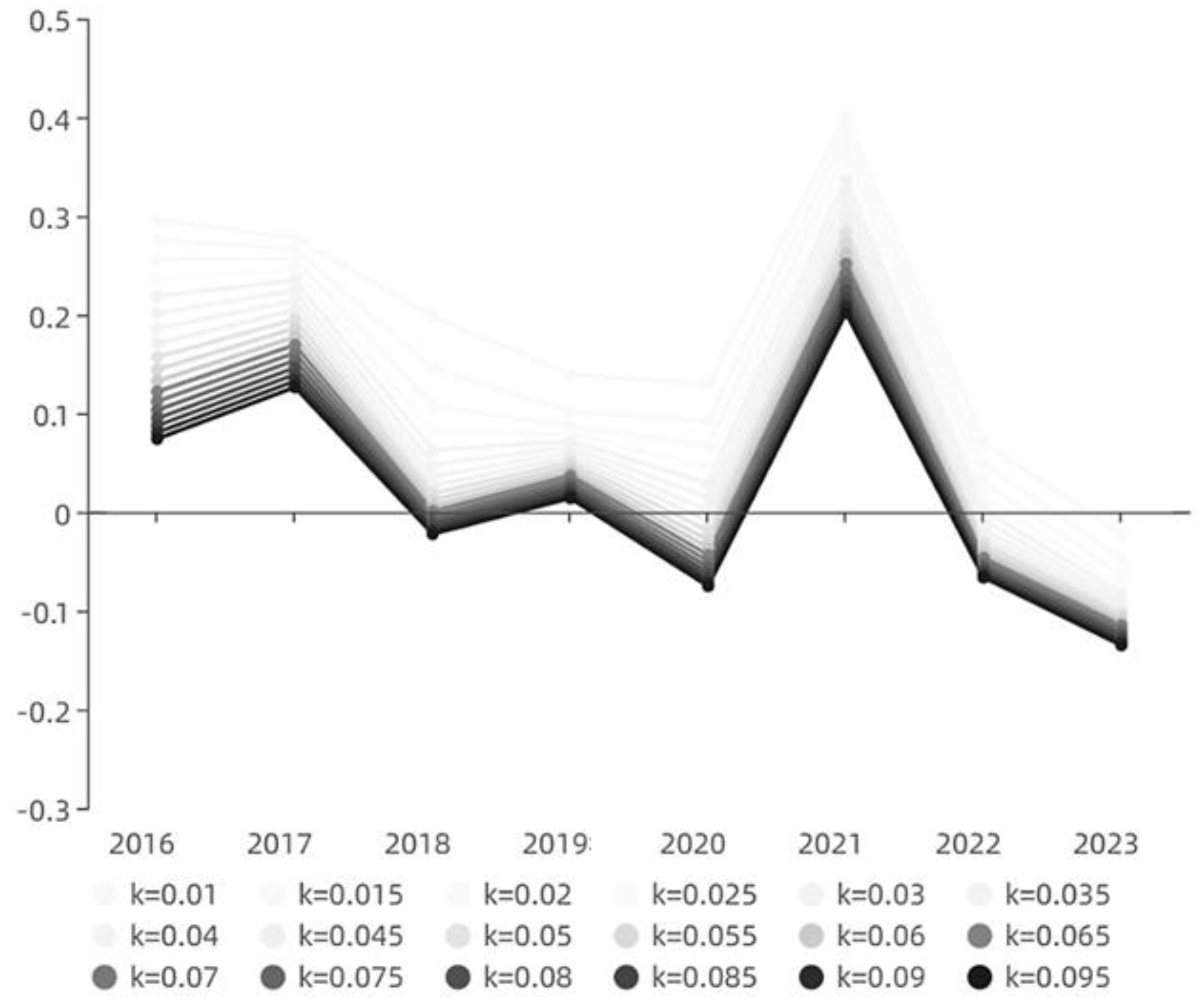
Table 15.
Comparison of the efficiency of the two models in calculating the growth rate of GGDP.
| Model | Target | Time complexity | Spatial complexity |
|---|---|---|---|
| GGDP model | Calculate the GGDP growth rate | ||
| GGDP growth rate correction model | Calculate the GGDP growth rate |
From the perspective of spatial complexity, the GGDP growth rate correction model using negative feedback moderation as the mechanism is more suitable than the GGDP model to calculate the GGDP growth rate, i.e., the modified GGDP growth rate, although the time complexity of both models is .
However, it is also advisable to use the GGDP model to calculate the GGDP growth rate, but the GGDP growth rate correction model not only makes up for the problems of high spatial complexity and excessive dependence on time lag data using the GGDP model, but also incorporates a negative feedback adjustment mechanism to make the results more robust.
Table 16.
Negative feedback adjustment mechanism of the GGDP growth rate correction model.
| Condition | Outcome |
|---|---|
| Both GDP and NER growth rates are stable | The growth rate of GGDP is stable |
| GDP and NER growth rates are at least one of them stable | The growth rate of GGDP has plateaued |
For different values, the growth rate of GGDP changes almost in a parallel trend, so does not affect the judgment of the change trend of the growth rate of GGDP, and there is no effect that the growth rate calculated by the GGDP model is not parallel to each other due to the fluctuation of the value. In the GGDP growth rate correction model, the larger the , the greater the negative feedback moderation effect, and the negative feedback adjustment mechanism is included to balance the promotion or inhibition of the NER growth rate and the GDP growth rate on the GGDP growth rate, so that the growth rate of GGDP can reduce the impact of the NER growth rate and the GDP growth rate instability as much as possible, and prevent the influence mechanism of "pseudo-promotion" and "pseudo-inhibition" on the GGDP growth rate caused by the instability of the NER growth rate or GDP growth rate (Tbl.12).
4.2. Robustness Analysis of the Double Helix Coupled Model (DHCM)
4.2.1. Robustness Analysis of Ecological Supply Capacity (E)
- From equation (20):
is an even number:
If , which is equal to , then ;
If , which is equal to , then .
When is an odd number:
If , which is equal to , then ;
If , which is equal to , then .
If , it shows that the elasticity coefficient of ecosystem factors has an increasing or unchanged interaction effect on ecological supply ability.
If , it indicates that the elasticity coefficient of ecosystem factors has a decreasing or unchanged interaction effect on ecological supply capacity.
4.2.2. Robustness Analysis of the Welfare Conversion Capacity (W)
If , then ;
If , then ;
If ,then.
indicates that the efficiency of the welfare conversion has an increasing or unchanged effect on the ability of the welfare transformation.
show that the efficiency of the welfare conversion has a decreasing or unchanged effect on the ability of the welfare transformation.
5. Conclusions and Recommendations
The GGDP and EWI development models of thirty-one provinces, cities and regions in China have obvious path dependence in terms of empirical results from 2015 to 2023, short-term projections from 2024 to 2030, and long-term projections from 2030 to 2060. If this inertia is not corrected, it will lead to uneven regional economic development while promoting regional economic development. To achieve the goals of carbon peak and carbon neutrality, it is necessary to take the sustainable development of the regional economy as the goal, which is embodied in (1) avoiding path dependence and (2) improving and maintaining a good regional economic development model.
(1) The GGDP growth rate model calculated by the negative feedback mechanism can reasonably measure the GGDP growth rate from 2016 to 2023, and this negative feedback mechanism eliminates the changes in GDP and NER growth rateThe rate of growth of the GGDP caused by the instability“Pseudo-facilitation”and“Pseudo-inhibition”impact.(2) According to the prediction results of CA Markov model, the development model of each province, city and region is still solidified, and the probability of supporting a low level of GGDP is 45.16%. However, the probability of the low-level state of GGDP jumping to the high-level state of GGDP is 35.49%, showing that the GGDP has still jumped from the low-level state to the high-level state of GGDP by changing the path dependence and inertia of development in many regions.
(1) The ecological supply function of the Lotka-Volterra symbiosis model (E) and the welfare conversion function (W) together "competition" and "cooperation", and finally found that no matter how E and W affect each other, their impact on EWI is positive, and the vast majority of provinces and regions W is at a high level, and E still has a lot of room for improvement.(2) There is obvious path dependence on the EWI development model in 31 provinces, cities and regions in China. Four provinces, Zhejiang, Jiangsu, Shandong and Guangdong, are at high GGDP, high EWI levels, indicating that Zhejiang, Jiangsu, Shandong, and Guangdong provinces are pioneers and model provinces for sustainable development in China.(3) 2030 predicted by the CA Markov model, The 2060 EWI level shows that if this path-dependent development pattern is not corrected, it will degrade provinces and regions with high EWI levels into medium or low EWI areas in the long run. According to the data, the proportion of low-level EWI regions will be 48.4% in 2030, and the proportion of low-level EWI areas will rise to 64.5% in 2060.
It is predicted that when achieving carbon peak and carbon neutrality, China will 31Most of the provinces, cities and regions will have a high level of GGDP levels, which are manifested as:(1) 2030 predicted by the CA Markov model In 2060, 61.3% of the GGDP will be at a high level.(2) if the level of ecological welfare is improved, especially the improvement of ecological supply capacity, Pathway dependence needs to be avoided, otherwise this pathway dependence will hinder the sustainable development of EWI over time.
References
- Talberth J , Bohara A K . Economic openness and green GDP[J]. Ecological Economics, 2006, 58(4):743-758. [CrossRef]
- Boyd J . The Non-Market Benefits of Nature: What Should Be Counted in Green GDP? [J]. Ecological Economics, 2006, 61(4):716-723.
- Li G, Fang C. Global mapping and estimation of ecosystem services values and gross domestic product: A spatially explicit integration of national ‘green GDP’accounting[J]. Ecological Indicators, 2014, 46: 293-314. [CrossRef]
- Sun F , Jia Z , Shen J ,et al. Research on the Accounting and Spatial Effects of Emergy Ecological Footprint and Industrial Green GDP--The Case of Yangtze River Economic Belt[J]. Ecological Indicators, 2024, 163(000):13. [CrossRef]
- Nahman A , Mahumani B K , Lange W J D . Beyond GDP: Towards a Green Economy Index[J]. Development Southern Africa, 2016, 33(2):215-233. [CrossRef]
- Liu Z , Guan D , Moore S ,et al. Climate policy: Steps to China's carbon peak[J]. Nature, 2015, 522(7556):279-281. [CrossRef]
- Yu Y, Yu M, Lin L, et al. National green GDP assessment and prediction for China based on a CA-Markov land use simulation model[J]. Sustainability, 2019, 11(3): 576. [CrossRef]
- Brajer V , Mead R W , Xiao F . Health benefits of tunneling through the Chinese environmental Kuznets curve (EKC)[J]. Ecological Economics, 2008, 66(4):674-686. [CrossRef]
- Wang J . Revive China's green GDP programme[J]. Nature, 2016, 534(7605):37-37. [CrossRef]
- Caviglia-Harris J L , Chambers D , Kahn J R . Taking the "U" out of Kuznets: A comprehensive analysis of the EKC and environmental degradation[J]. Ecological Economics, 2009, 68(4):1149-1159.
- Tang Shaoxiang,Guo Zhi,Zhou Xinmiao. Research on sustainable development of China's economy:green accounting and empirical analysis[M].Shanghai Jiao Tong University Press,2016:63-73.
- FANG Shijiao,XIAO Quan. Study on regional ecological welfare performance level and its spatial effect in China[J].Chinese Population, Resources and Environment, 2019, 29(003):1-10.).
- DONG Ying,SUN Yuhuan,DING Jiao. Acta Geographica Sinica, 2024, 79(5):1337-1354.
- ZANG Mandan,ZHU Dajian,LIU Guoping. Ecological welfare performance: concept, connotation and G20 empirical evidence[J].Chinese Population, Resources and Environment, 2013, 23(5):7.
- Costanza R, d'Arge R, De Groot R, et al. The value of the world's ecosystem services and natural capital[J]. Nature, 1997, 387(6630): 253-260. [CrossRef]
Figure 2.
Empirical results of the GGDP model
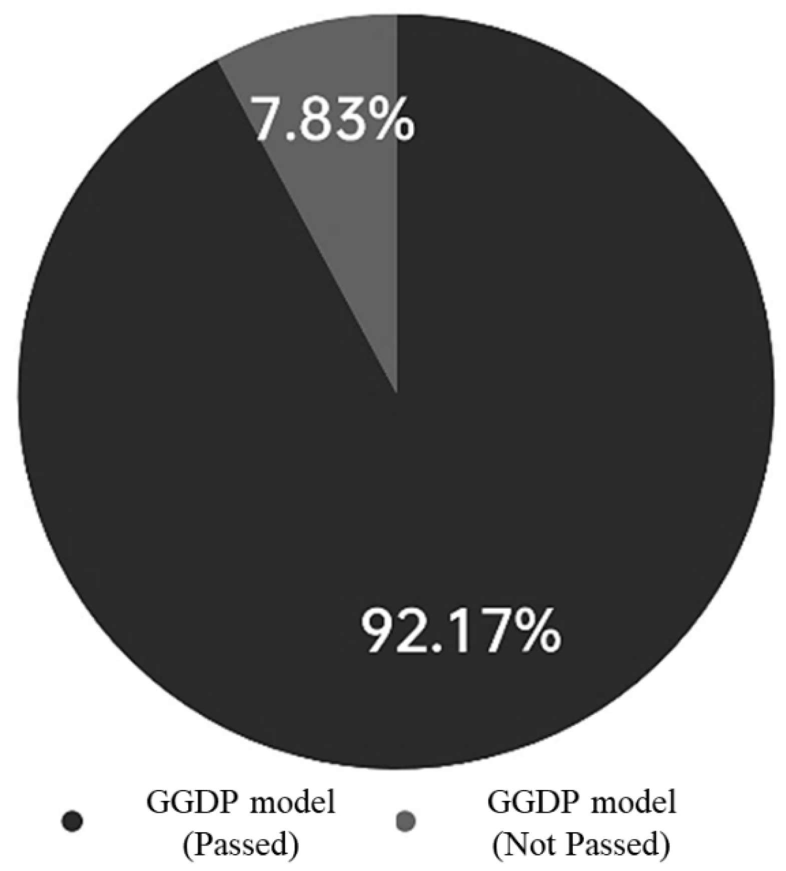
Figure 3.
The NER of 31 provinces, cities and regions in China satisfies Ziff's law.
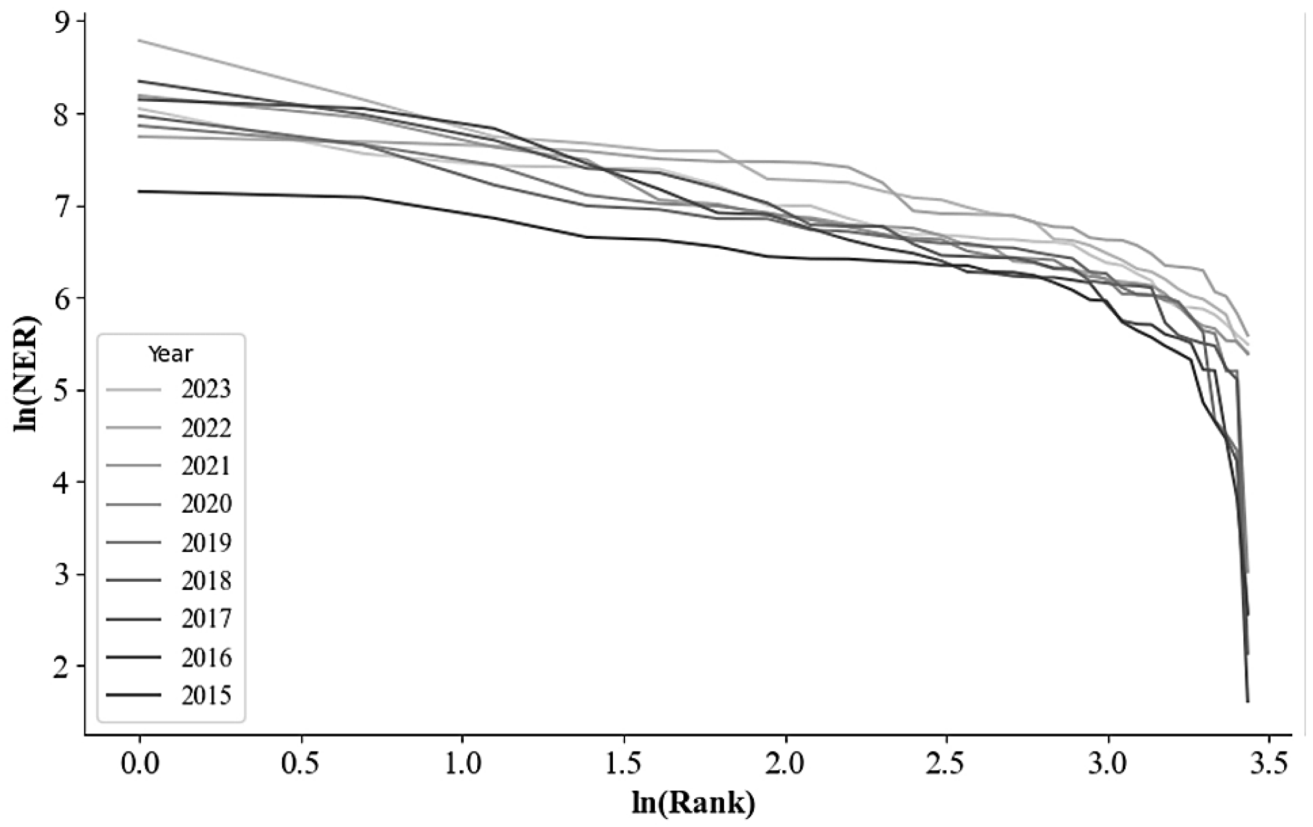
Figure 4.
Growth rates of GGDP, GDP and NER of 31 provinces, cities and regions from 2016 to 2023.(Note: The abscissa represents the province, city and region, and the ordinate is the percentage)
Figure 4.
Growth rates of GGDP, GDP and NER of 31 provinces, cities and regions from 2016 to 2023.(Note: The abscissa represents the province, city and region, and the ordinate is the percentage)
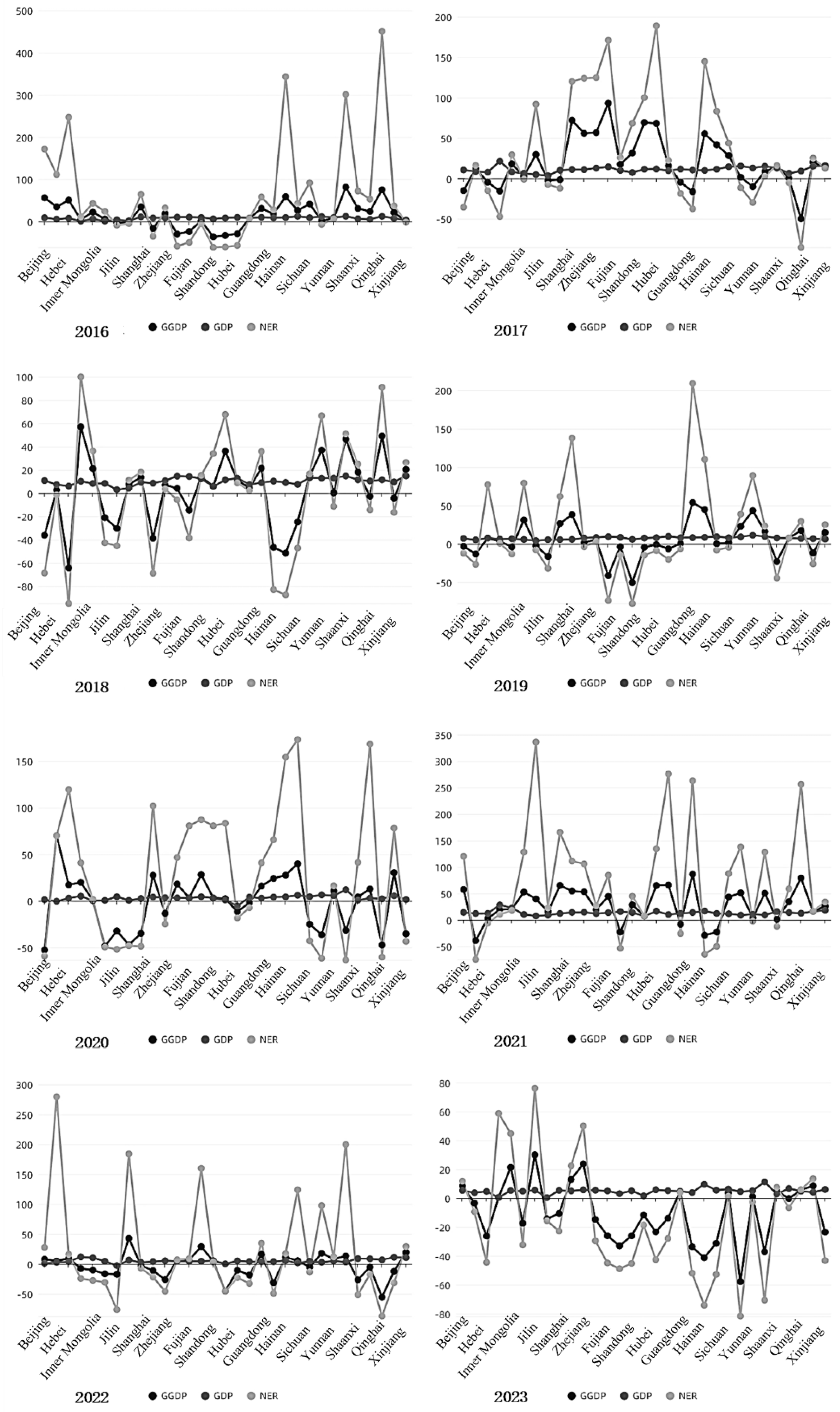
Figure 5.
Correlation coefficient between NER and GGDP from 2016 to 2023 ().
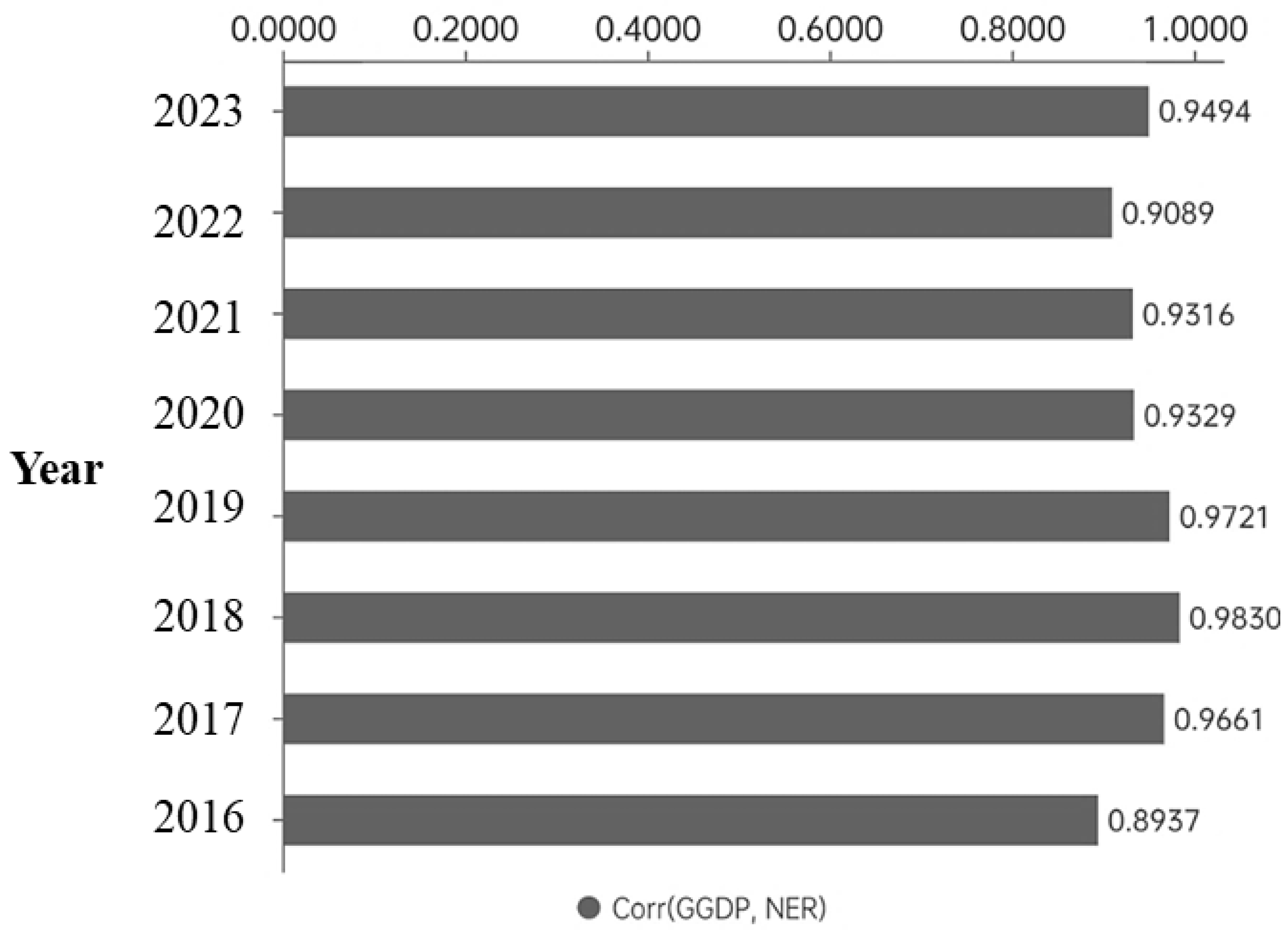
Figure 6.
The GGDP of 31 provinces, cities and regions in China satisfies Zif's law.
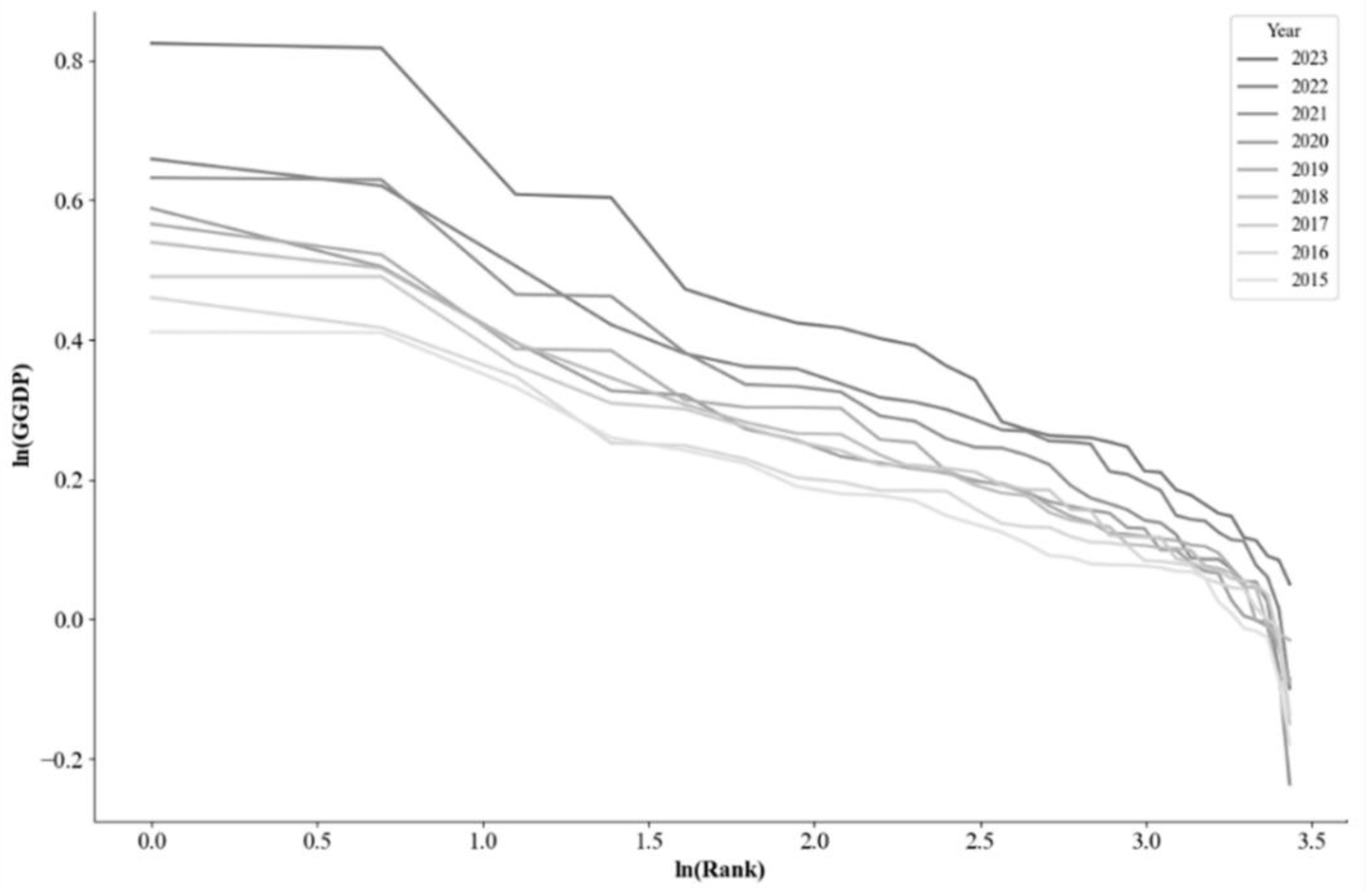
Figure 7.
SI () in thirty-one provinces, cities and regions in China from 2015 to 2023
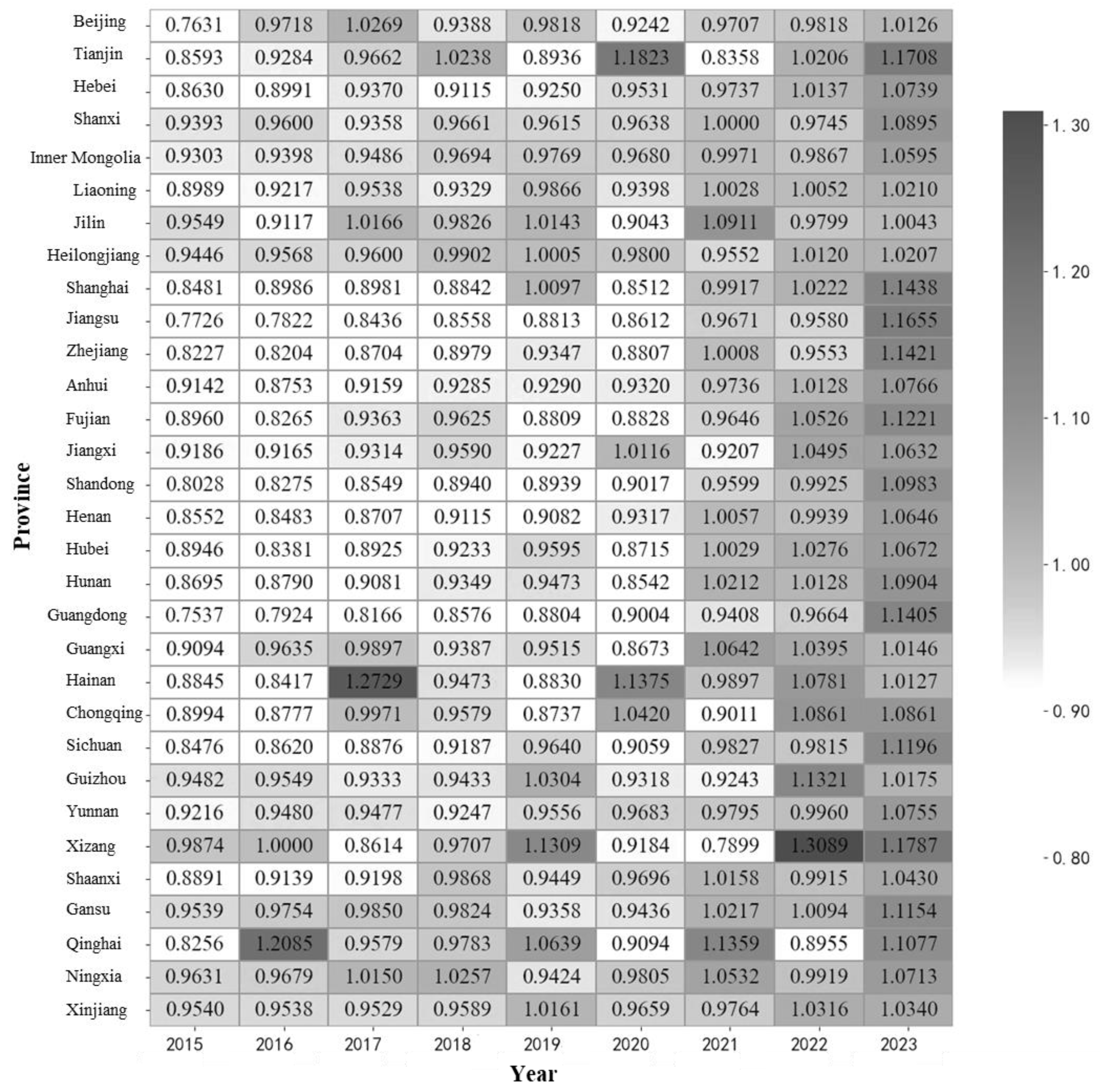
Figure 8.
Load chart of green GDP index and ecological welfare index of 31 provinces, cities and regions in China from 2019 to 2023.
Figure 8.
Load chart of green GDP index and ecological welfare index of 31 provinces, cities and regions in China from 2019 to 2023.
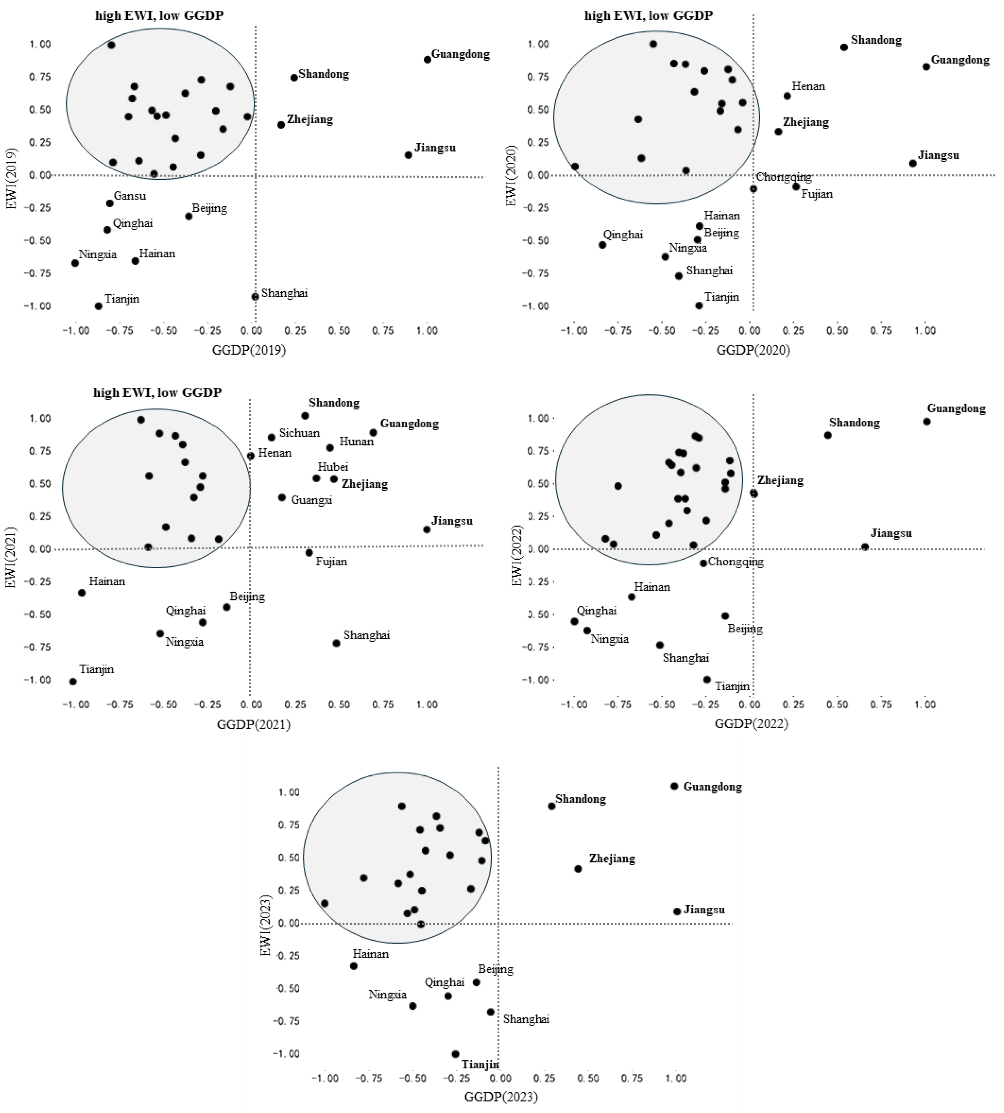
Figure 9.
Ecology (E) and the welfare (W) loads in thirty-one provinces, cities and regions in China from 2019 to 2023.
Figure 9.
Ecology (E) and the welfare (W) loads in thirty-one provinces, cities and regions in China from 2019 to 2023.
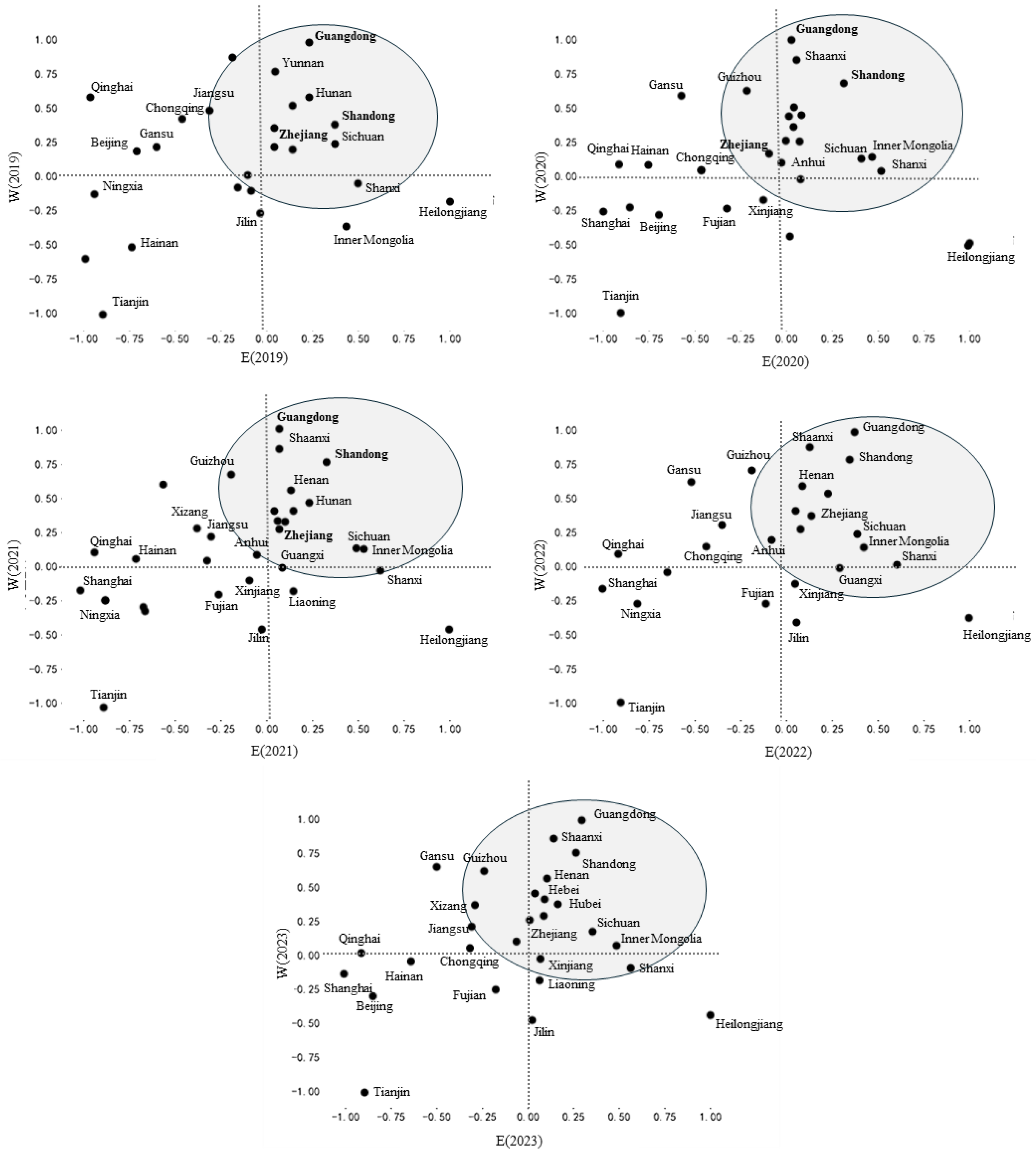
Figure 10.
CA Markov model predicts the GGDP and EWI level category counts in each region in 2030.
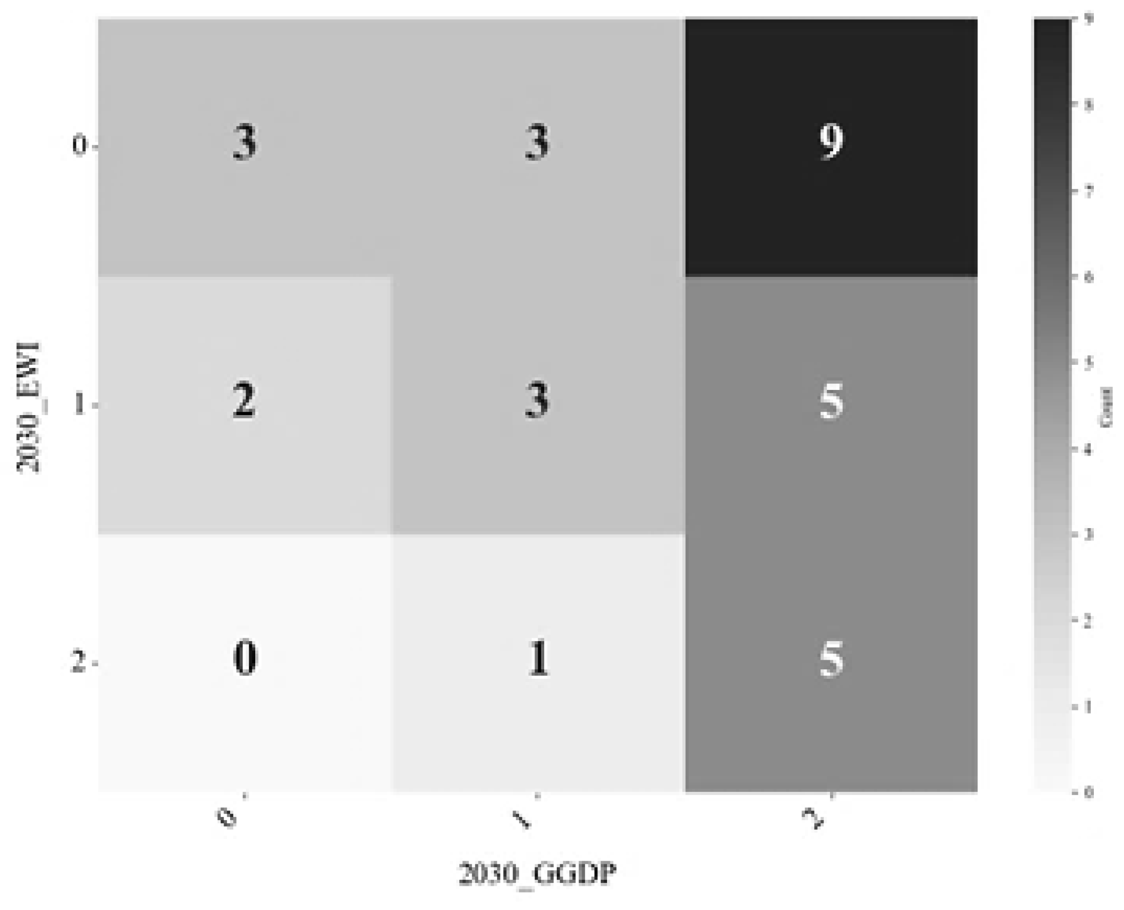
Figure 11.
CA Markov model predicts the levels of GGDP and EWI in each region in 2060.
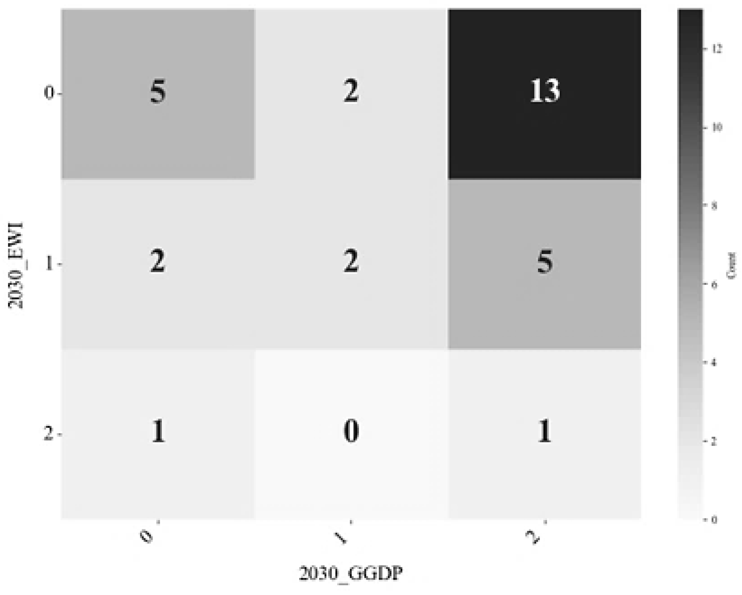
Figure 12.
Trends in the average GGDP of each province and region from 2015 to 2023
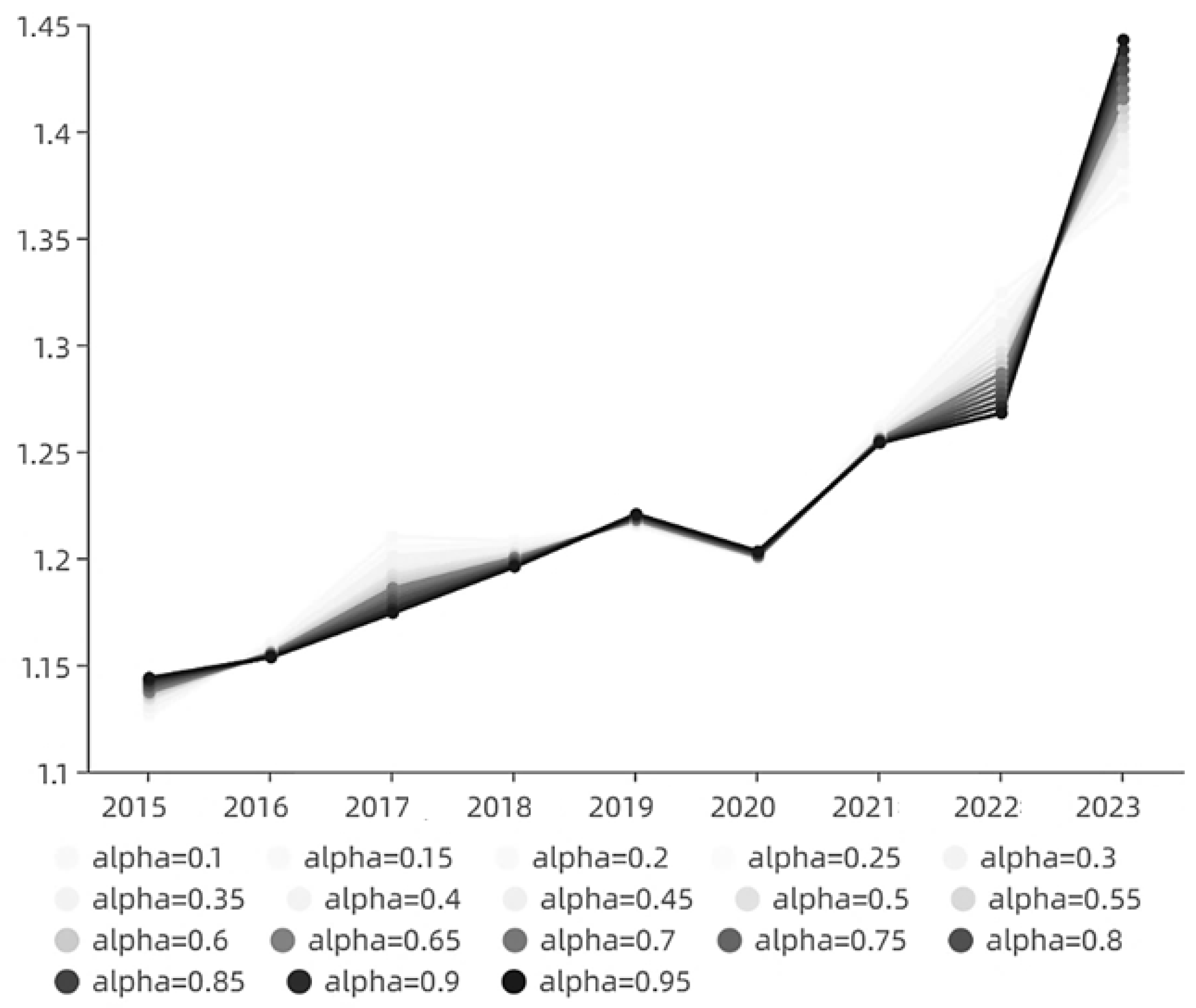
Table 2.
Regression results of NER and ranking satisfying Ziff's law.
| Argument | Dependent variable | Factors not normalized | Normalization factor | |
| Ln (Rank) | Ln (2015_NER) | -0.850(***) | -0.740(***) | 0.548 |
| Ln (2016_NER) | -1.173(***) | -0.810(***) | 0.656 | |
| Ln (2017_NER) | -1.047(***) | -0.812(***) | 0.659 | |
| Ln (2018_NER) | -0.921(***) | -0.755(***) | 0.570 | |
| Ln (2019_NER) | -0.835(***) | -0.806(***) | 0.650 | |
| Ln (2020_NER) | -0.797(***) | -0.976(***) | 0.952 | |
| Ln (2021_NER) | -0.614(***) | -0.897(***) | 0.805 | |
| Ln (2022_NER) | -0.874(***) | -0.960(***) | 0.921 | |
| Ln (2023_NER) | -0.699(***) | -0.951(***) | 0.903 |
Table 3.
GGDP, GDP and NER results of the Yangtze River Delta urban agglomeration in 2023.
| Yangtze River Delta urban agglomeration | GGDP | GDP | DOWN | |||
|---|---|---|---|---|---|---|
| Shanghai | 1.5285 | -10.55% | 1.3363 | 5.38% | 1.4904 | -22.80% |
| Jiangsu | 2.2659 | 12.96% | 1.9441 | 5.02% | 1.1723 | 22.40% |
| Anhui | 1.4374 | -14.81% | 1.3351 | 5.48% | 1.1780 | -29.54% |
| Zhejiang | 1.8290 | 23.69% | 1.6014 | 5.76% | 1.1930 | 50.05% |
Table 4.
Results of GGDP, GDO and NER of the Beijing-Tianjin-Hebei urban agglomeration in 2023.
| Beijing-Tianjin-Hebei urban agglomeration | GGDP | GDP | DOWN | |||
|---|---|---|---|---|---|---|
| Beijing | 1.3269 | 8.47% | 1.3104 | 5.34% | 1.1910 | 11.79% |
| Tianjin City | 1.1268 | -3.44% | 1.1076 | 3.75% | 2.0000 | -9.47% |
| Hebei | 1.4087 | -26.24% | 1.3118 | 4.66% | 1.0416 | -44.48% |
Table 5.
GGDP, GDP and NER results of Chengdu-Chongqing urban agglomeration in 2023
| Chengdu-Chongqing urban agglomeration | GGDP | GDP | DOWN | |||
|---|---|---|---|---|---|---|
| Sichuan | 1.6046 | 3.74% | 1.4332 | 6.22% | 1.1786 | 1.36% |
| Chongqing | 1.3122 | -31.21% | 1.2082 | 5.49% | 1.2939 | -52.80% |
Table 6.
GGDP, GDP and NER results of the urban agglomeration in the middle reaches of the Yangtze River in 2023.
Table 6.
GGDP, GDP and NER results of the urban agglomeration in the middle reaches of the Yangtze River in 2023.
| Urban agglomeration in the middle reaches of the Yangtze River | GGDP | GDP | DOWN | |||
|---|---|---|---|---|---|---|
| Hubei | 1.4949 | -23.32% | 1.4007 | 5.81% | 1.1707 | -42.53% |
| Hunan | 1.4800 | -13.96% | 1.3573 | 5.16% | 1.2138 | -27.84% |
| Jiangxi | 1.3009 | -32.95% | 1.2236 | 3.16% | 1.1650 | -48.82% |
Table 7.
GGDP, GDP and NER results of the Beibu Gulf urban agglomeration in 2023
| Beibu Gulf urban agglomeration | GGDP | GDP | DOWN | |||
|---|---|---|---|---|---|---|
| Guangxi | 1.2035 | -33.61% | 1.1861 | 3.88% | 1.0835 | -51.89% |
| Guangdong | 2.2809 | 4.35% | 2.0000 | 4.76% | 1.1141 | 3.94% |
| Hainan | 1.0519 | -41.22% | 1.0387 | 9.60% | 1.0204 | -74.09% |
Table 8.
Regression results of GGDP and ranking satisfying Ziff's law.
| Argument | Dependent variable | Regression coefficients | Normalization factor | |
| Ln (Rank) | Ln (2015_GGDP) | -0.145*** | -0.951*** | 0.905 |
| Ln (2016_GGDP) | -0.139*** | -0.963*** | 0.928 | |
| Ln (2017_GGDP) | -0.152*** | -0.951*** | 0.904 | |
| Ln (2018_GGDP) | -0.161*** | -0.987*** | 0.974 | |
| Ln (2019_GGDP) | -0.172*** | -0.972*** | 0.944 | |
| Ln (2020_GGDP) | -0.173*** | -0.971*** | 0.942 | |
| Ln (2021_GGDP) | -0.205*** | -0.946*** | 0.894 | |
| Ln (2022_GGDP) | -0.184*** | -0.959*** | 0.920 | |
| Ln (2023_GGDP) | -0.229*** | -0.988*** | 0.976 |
Table 9.
Classification results of the Sustainable Development Index (SI).
| Classification factor | Classification criteria | Category name |
|---|---|---|
| 0 | Low | |
| 1 | Moderate | |
| 2 | High |
Table 13.
Classification results of the Ecological welfare Index (EWI).
| Classification factor | Classification criteria | Category name |
|---|---|---|
| 0 | Low | |
| 1 | Moderate | |
| 2 | High |
Table 14.
EWI transfer matrix from 2023 to 2030/2060.
| EWI | 2030/2060 | |||
|---|---|---|---|---|
| 0 | 1 | 2 | ||
| In 2023 | 0 | 0.9500 | 0.0500 | 0.0000 |
| 1 | 0.1429 | 0.8095 | 0.0476 | |
| 2 | 0. 0000 | 0.1190 | 0.8810 | |
| 1 | DONG Han,ZOU Minghua,LI Lu,LI Yan. Correlation and prediction analysis of green GDP accounting based on SEEA[J].Bulletin of Soil and Water Conservation,2024,44(2):187-195,204.) |
| 2 | Kravchenko Maryna,Trofymenko Olena,Kopishynska Kateryna,et al. Ensuring energy security on the basis of intelligent decarbonisation and innovative economic development[J]. E3S THE PAPERB OF CONFERENCES,2024,558. |
| 3 | Renewable Resources and Circular Economy,2021,14(12):43 |
| 4 | |
| 5 | |
| 6 | |
| 7 | |
| 8 | |
| 9 | Gao Yunhong,Zhang Yanshu,Yang Mingjie. 20 Years of Western Development: Northwest vs. Southwest[J]. Regional Economic Review,2020(5):36-51. |
| 10 | Gansu Provincial Forestry and Grassland Bureau 2023 Forestry and Grassland Ecological Protection and Restoration Fund Performance Self-Assessment Report |
| 11 | |
| 12 | In order to eliminate the influence of dimensions, all data in the empirical analysis module are interpolated, with regions ranging from 1 to 2. |
| 13 | |
| 14 |
Disclaimer/Publisher’s Note: The statements, opinions and data contained in all publications are solely those of the individual author(s) and contributor(s) and not of MDPI and/or the editor(s). MDPI and/or the editor(s) disclaim responsibility for any injury to people or property resulting from any ideas, methods, instructions or products referred to in the content. |
© 2025 by the authors. Licensee MDPI, Basel, Switzerland. This article is an open access article distributed under the terms and conditions of the Creative Commons Attribution (CC BY) license (http://creativecommons.org/licenses/by/4.0/).
Copyright: This open access article is published under a Creative Commons CC BY 4.0 license, which permit the free download, distribution, and reuse, provided that the author and preprint are cited in any reuse.


