
Submitted:
05 May 2025
Posted:
06 May 2025
You are already at the latest version
Abstract
This study presents a probabilistic geotechnical analysis of the Visonta Keleti-III lignite mining area, focusing on the statistical evaluation of soil parameters and their integration into slope stability modeling. The objective was to provide a more accurate representation of the spatial variability of geological formations and mechanical soil pro-perties, in contrast to traditional deterministic approaches. The analysis was based on over 3,300 laboratory samples from 28 boreholes, processed through multi-stage outlier filtering and regression techniques. Strong correlations were identified between physical soil parameters—such as wet and dry bulk density, void ratio, and plasticity index—particularly in cohesive soils. The probabilistic slope stability analysis applied the Bishop simplified method in combination with Latin Hypercube simulation. Results demonstrate that traditional methods tend to underestimate slope failure risk, whereas the probabilistic approach reveals failure probabilities ranging from 0% to 46.7% across different sections. The use of tailored statistical tools—such as Python-based filtering algorithms and distribution fitting via MATLAB—enabled more realistic modeling of geotechnical behavior. The findings emphasize the necessity of statistical methodologies in mine design, particularly in geologically heterogeneous, multilayered environments, where spatial uncertainty plays a critical role in slope stability assessments.
Keywords:
statistical analysis
; complex geology
; open pit mining
; probabilistic slope stability analysis
1. Introduction
The statistical evaluation of soil parameters is of fundamental importance in slope stability analysis, as the physical and mechanical properties of soil exhibit significant spatial variability. Traditional slope stability analysis methods, such as limit equilibrium approaches, cannot always take into account these uncertainties. Modern approaches, such as Monte Carlo simulation, provide an opportunity for the quantitative estimation and integration of these uncertainties into the design process. [1,2] Uncertainties in shear strength parameters such as soil cohesion and internal friction angle influence safety factors. Monte Carlo simulation enables the implementation of probabilistic analyses, allowing the modeling of the effects of various soil parameters. [3,4]
The natural anisotropy of soils, which develops during particle deposition, fundamentally influences slope stability. Traditional isotropic models may significantly overestimate safety factors, whereas considering anisotropy allows for more accurate results. [4,5] Numerical methods, such as the Finite Elements Method (FEM) and the Discrete Elements Method (DEM), can account for the spatial variability of the mechanical properties of soil and rock. Probabilistic analysis techniques, such as the Strength Reduction Techniques (SRT) method, enable a detailed investigation of slope instability processes. [6,7] Statistically based evaluation techniques assist in determining optimal design parameters, thereby reducing the risk of underestimated instability. These methods can be applied to the design of earth dams, mining slopes, as well as road and railway embankments. [3] [7] Integrating these approaches into the engineering design process facilitates the development of safer and more cost-effective solutions. It is necessary to understand the impact of soil parameter variability and explore potential risk reduction strategies. Probabilistic modeling is a method that accounts for the uncertainty associated with input parameters during analysis, yielding the statistical distribution of the Factor of Safety (FS) instead of a single deterministic value. The resulting probability of failure (PF) has become a widely accepted design criterion. [8 - 10] The basis of the Probability of Failure (PF) concept is the determination of a statistical distribution (probability density function) for each input parameter in a slope stability analysis. The statistical distribution of the Factor of Safety (FS) can be established using a stochastic simulation process. PF quantifies the percentage of cases where FS < 1, indicating potential failure. Soil mechanical analyses often encounter the inherent uncertainty of soil parameters, which significantly impacts slope stability. To account for uncertain soil parameters, researchers have applied a probabilistic approach that has proven to be an effective tool when combined with Monte Carlo or Latin Hypercube simulation and Bishop’s simplified method. The analysis examined critical slip surfaces and the factor of safety, highlighting that probabilistic modeling of soil strength improvements and groundwater levels can significantly reduce the risk of slope failure. [11] Natural soil deposition processes often lead to strength anisotropy, which, if neglected, can result in inaccurate slope stability assessments. In the study of He et al. (2022) [12] a generalized anisotropic model was applied to describe the directional variations in the soil’s friction angle. The results indicate that ignoring anisotropy can overestimate the stability factor by up to 32.9%, particularly in the case of gentler slopes. The study emphasizes the importance of explicitly considering soil strength anisotropy to achieve more accurate stability assessments. [12] The stability of mining slopes is of paramount importance due to safety, economic, and environmental considerations. A Synthetic Rock Model (SRM) study aimed to simulate various geological layers and discontinuities accurately. Discrete Elements Methods (DEM) and Strength Reduction Techniques (SRT) enabled a detailed examination of sliding mechanisms. The results confirmed that these numerical models effectively predict the stability of complex geological environments, particularly in identifying slip surfaces and instability processes. [13] This study presents a comprehensive statistical evaluation of soil parameters and a probabilistic slope stability analysis of the Visonta lignite mining area in Hungary, highlighting how advanced data filtering, distribution fitting, and Latin Hypercube simulations can effectively capture the uncertainty of geotechnical parameters and provide a more realistic assessment of slope safety, ultimately revealing an estimated failure probability for one of the critical mining sections.
2. Geological Settings and Geotechnical Parameters
2.1. Geographical Location
Visonta is located in North Hungary, at the southern foothills of the Northern Medium Mountains, east of Gyöngyös. (Figure 1) The Visonta mining site, based on lignite extraction, is located on the northern edge of the Great Hungarian Plain, at the southern foothills of the Mátra Mountains (Figure 2). Since the 1970s, multiple open-pit mining operations have been carried out in the region, utilizing the Visonta lignite deposit. The mining area is a key part of the Northern Hungarian lignite region. Geological research conducted in the 1960s and 1970s indicated that the Mátra and Bükkalja regions contain hundreds of millions of tons of extractable mineral resources, suitable for long-term energy utilization. Geomorphologically, the area is highly diverse and can be classified as a low hill region. Its topography is characterized by decreasing slopes towards the south and rising ridges towards the northwest. The highest part of the mining site, located in the northeastern section, varies between 160 and 180 meters above sea level, while its lowest point lies at an elevation of 115 meters above sea level in the valley of the Tarnóca Creek.
2.2. Interburden and Overburden Layer Characteristics
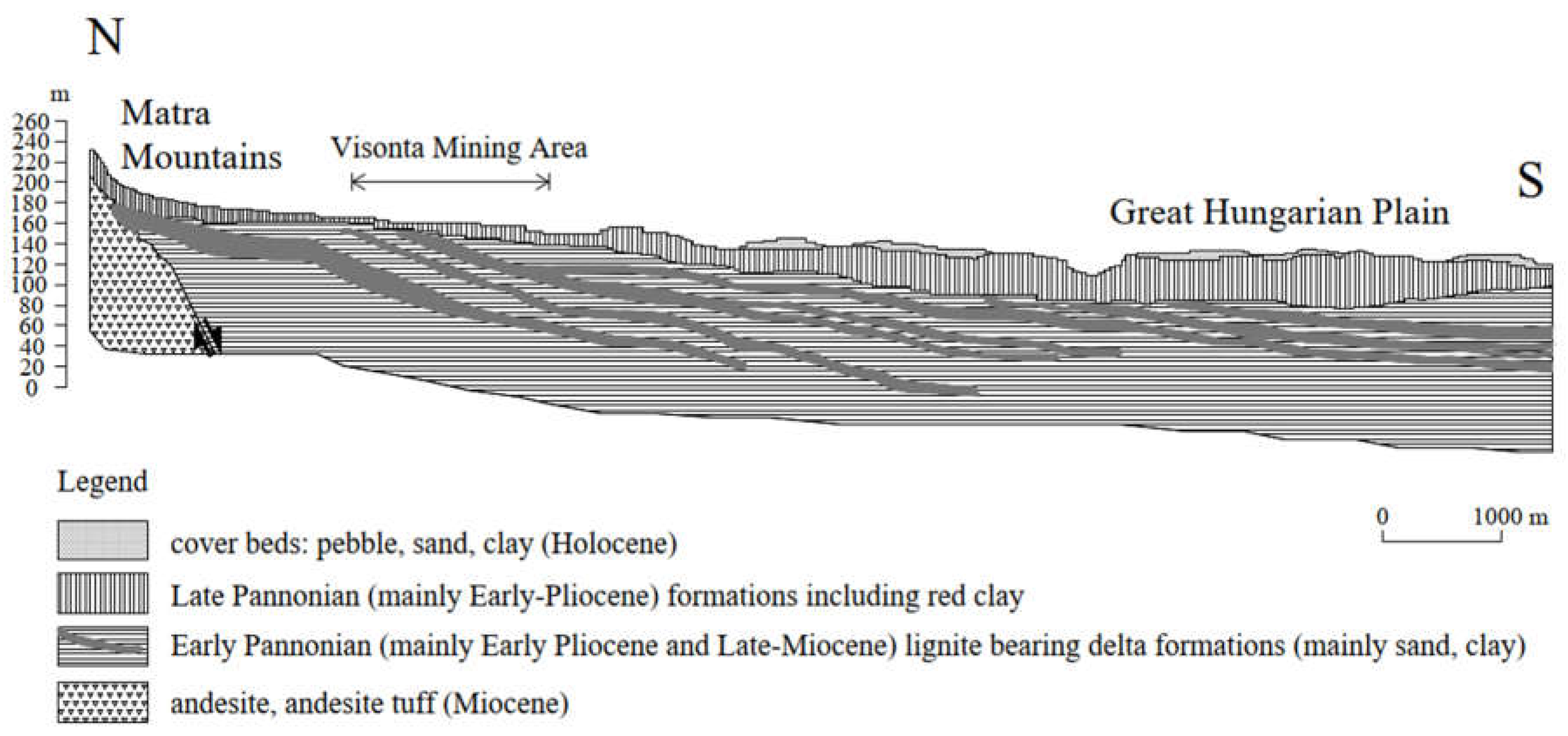
The overburden above the uppermost coal seam and the interbeds between the individual coal seams consist of loose sediments. The Late Pannonian formation, containing the lignite seams, is overlain by a Quaternary overburden of varying thickness. This overburden consists primarily of various materials, including dark brown, red, reddish brown, yellowish brown, grey, yellow and black bentonite deposits, often with limestone concentrations and occasionally with limonite and manganese content. In some areas, a sandy clayey gravel layer can be observed. Some clayey materials have a mosaic structure, which breaks into small (walnut-sized) shiny-surfaced fragments after the loss of the substrate. The thickness of the Quaternary overburden ranges from 5 to 50 m, showing an increasing trend from north to south. The Cserhát–Mátra–Bükkalja lignite-bearing sequence is overlain by inland sand, silt and clay layers, occasionally interbedded with lignite seams. The coal layers within the sequence are separated by clay and sand layers. In some places, sandstone layers and compact marly silts represent significant resistance to mining.
Figure 2.
Geological Cross-Section from the Mátra Mountains to the Great Hungarian Plain Across the Visonta Mining Area after Horváth et al. (2005) [14].
Figure 2.
Geological Cross-Section from the Mátra Mountains to the Great Hungarian Plain Across the Visonta Mining Area after Horváth et al. (2005) [14].
2.3. Geological Structure of Lignite Layers
The lignite deposits are found in Pliocene formations, which are overlain by Quaternary cover layers. (Figure 3) The structural setting of the area is basin-like, with a basement composed of Miocene andesite formations of the Mátra Mountains. Overlying this basement is a several hundred-meter-thick Pliocene sedimentary sequence, with its Late Pannonian section containing the lignite seams. The sedimentary sequence is characterized by relatively stable depositional conditions, with a general dip direction of NW-SE at an average inclination of 2–3°. Due to variations in stratigraphic dip, some lignite seams extend to the denuded surface of the Late Pannonian formations, where they have been partially eroded. The individual coal seams show significant differences in thickness, quality, and structural characteristics. These lignite seams belong to the Bükkalja Lignite Formation, deposited during the Late Pannonian epoch of the Tertiary period. Sediments accumulated in a shallow basin, fed by weathering products from surrounding mountains. Over time, delta slope facies evolved into floodplain and fluvial-lacustrine deposits, filling the basin by the epoch's end. Swamps and peatlands formed along basin margins, giving rise to lignite seams from Taxodium swamp forests. [15]
Figure 4 displays two geological cross-sections from the Visonta Keleti-III lignite mining area, showing stratigraphic layering based on borehole data. Multiple sedimentary units are represented, including various clays (e.g., fat clay or high plasticity clay, medium plasticity clay, organic and bentonitic clays), silts, silty clays, and lignite seams. Strata are shown with distinct colors. The lignite seams are interbedded with fine-grained sediments and occur at varying depths across sections. Upper layers are predominantly composed of fat clays and silts, while deeper units include high-plasticity and organic clays. The aquifer units consist of granular soils, predominantly sandy layers.
2.4. Geotechnical Investigations and Stability Calculations
Several investigatory drillings have been made in the area. The geological logs were obtained, containing the identified stratigraphic layers from individual boreholes, along with detailed sample descriptions, age determinations, depth data, sample types, and corresponding sample numbers. These reports contained information such as borehole name, layer name, soil sample color, material characteristics, other relevant properties, layer depth, sample age, and sample number. For disturbed samples, the following parameters were determined: liquid limit (wL), plastic limit (wP), relative consistency index (Ic), plasticity index (Ip), and grain size frequency distribution characteristics—percentage distribution of gravel, sand, silt, and clay, as well as characteristic grain diameter (Dm), uniformity coefficient (Cu), and grain size parameters (D10, D20, D60). For undisturbed samples, the available data included water content (w), void ratio (e), degree of saturation (Sr), dry bulk density (rd), and wet bulk density (rn). Certain samples underwent shear testing, and results were provided as average values measured on a horizontal shear plane. From these tests, the cohesion values, as well as internal friction angles, were determined. A total of 28 boreholes, drilled between 1988 and 2008 in the Visonta Keleti-III mining area, were examined during the current research. The bore-holes are documented with known drilling dates, EOV (X) and EOV (Y) coordinates, height above sea level, and drilling depths. Table 1 shows the number of all the laboratory tests completed on soil samples from Visonta mining area.
3. Methodology
After examining the data of the 28 boreholes and more than 3300 samples from the Visonta Keleti-III mining area, soil classification was performed based on plasticity index and grain size distribution results. After the classification, statistical analyses were performed focusing on two main categories: shear strength parameters, unit weight, and physical soil parameters. Ultimately, the collected data were used for probabilistic slope stability analysis. The workchart for the investigation is on Figure 5.
3.1. Methodology of Correlation Analysis
A total of thirteen soil types were analysed: clayey Sand (clSa), clayey Silt (clSi), Sand (Sa), sandy Clay (saCl), sandy clayey Silt (saclSi), sandy Silt (saSi), sandy silty Clay (saclSi), sandy Gravel (saGr), Silt (Si), silty Sand (siSa), high plasticity Clay, medium plasticity Clay, and low plasticity Clay.
Relationships were examined between the following parameters: wet bulk density and void ratio, dry bulk density and void ratio, wet bulk density and dry bulk density and plasticity index and liquid limit. The study was conducted in three phases. The first phase served as a baseline, where all available laboratory results for each parameter related to each soil type were included.
Subsequently, outlier values were filtered for each soil type and for each studied soil parameter using manual, basic filtering based on the Interquartile Range (IQR) method. The IQR filtering method is used to remove data points that significantly differ from the rest, known as outliers. The central part of the data is identified, and the range between the lower and upper quartiles is measured. Based on this range, boundaries are determined, and any values falling outside these limits are excluded, as they are considered unusual or potentially incorrect. This procedure can be performed in Python, and from Microsoft Excel 2016 onwards, the quartile function is also supported for this purpose.
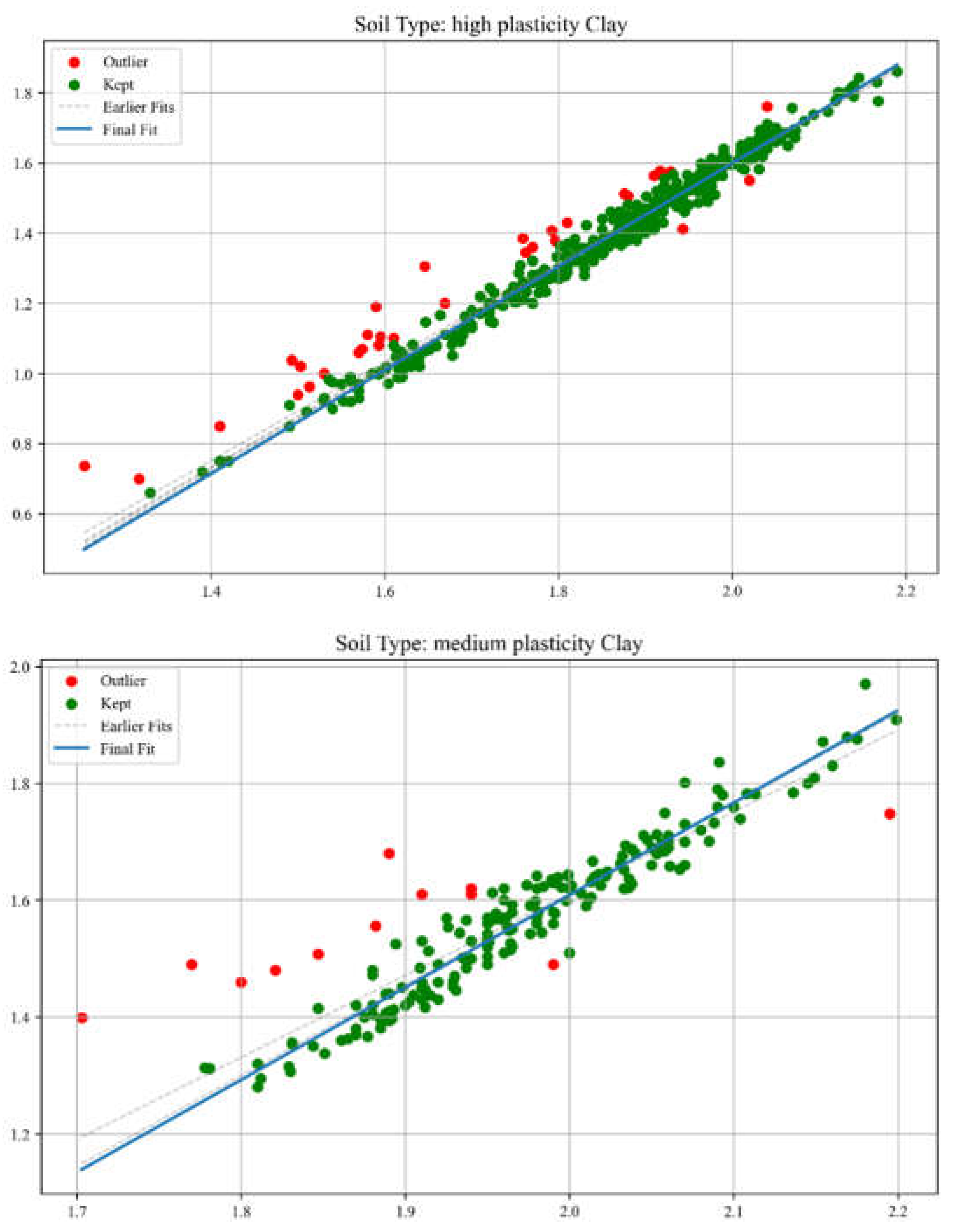
The same procedure was later carried out using a more professional and efficient approach—dynamical filtering—implemented through Python code. The Python program performs iterative outlier detection and visualization on soil-related experimental data. It applies linear regression within each soil type group and iteratively removes statistical outliers based on interquartile range (IQR) analysis of residuals. Each iteration’s regression line is recorded: all intermediate fits are shown as dashed grey lines, while the final fit is highlighted in bold. The tool facilitates reproducible and transparent data cleaning for soil parameter analyses. Dashed grey lines represent earlier regression fits, while the final regression model is shown as a solid blue line. This method allows for very accurate data filtering but carries the risk of excessive data loss. The amount of data lost is shown in Table 2. The simple filter called IQR filtering with MS Excel was used during the research, since too much data loss can have negative consequences because it reduces the representativeness of the data.
Figure 6.
Regression Fit and Outlier Filtering (examples of dynamical filtering method).
The essential part of the Python script code has been highlighted below.
def iterative_outlier_filtering(group):
group = group.copy()
all_outliers = []
regression_lines = []
num_iterations = 0
while True:
if len(group) < 2:
break
slope, intercept, _, _, _ = linregress(group['Value1'], group['Value2'])
regression_lines.append((slope, intercept))
num_iterations += 1
group['Predicted_Value2'] = group['Value1'] * slope + intercept
group['Residual'] = group[' Value2'] - group['Predicted_ Value2']
q1 = group['Residual'].quantile(0.25)
q3 = group['Residual'].quantile(0.75)
iqr = q3 - q1
lower_bound = q1 - 1.5 * iqr
upper_bound = q3 + 1.5 * iqr
group['Outlier'] = ~group['Residual'].between(lower_bound, upper_bound)
outliers = group[group['Outlier']]
if outliers.empty:
break
all_outliers.append(outliers)
group = group[~group['Outlier']]
group['Outlier'] = False
if all_outliers:
all_outliers_df = pd.concat(all_outliers)
all_outliers_df['Outlier'] = True
final_group = pd.concat([group, all_outliers_df])
else:
final_group = group
final_group = final_group.sort_index()
final_slope, final_intercept = regression_lines[-1] if regression_lines else (0, 0)
return final_group, final_slope, final_intercept, regression_lines, num_iterations
3.1. Methodology of the Statistical Analysis
In probabilistic slope stability analysis, accurately defining the statistical properties of input parameters is essential. This includes determining the appropriate probability distribution, mean, standard deviation, and range. These parameters ensure that variability is realistically captured in the model. The analysis in this study uses Rocscience software, which limits inputs to seven distribution types: Normal, Lognormal, Triangular, Gamma, Beta, Uniform, and Exponential. Hence, selecting the most representative distribution for each parameter is critical. A custom MATLAB script was developed specifically for this study. It focuses on the seven distributions supported by Rocscience. By estimating parameters, the script fits multiple distributions: normal, lognormal, exponential, gamma, beta, uniform, and triangular. Each model is evaluated using log-likelihood and the Akaike Information Criterion (AIC), which balances model fit with complexity. The best-fitting model is identified based on the lowest AIC value. Visualization includes a histogram with overlaid probability density functions (PDFs) for each distribution, each plotted in a distinct color.
The best-fitting model is emphasized with a thicker line and annotated with the distribution name, AIC, mean, and standard deviation. For improved usability and validation, a parallel Python implementation was created. It mirrors the MATLAB version but includes more robust error handling and input validation.
Figure 7.
Comparison of Probability Distribution Fits Using Matlab (a) and Python (b).
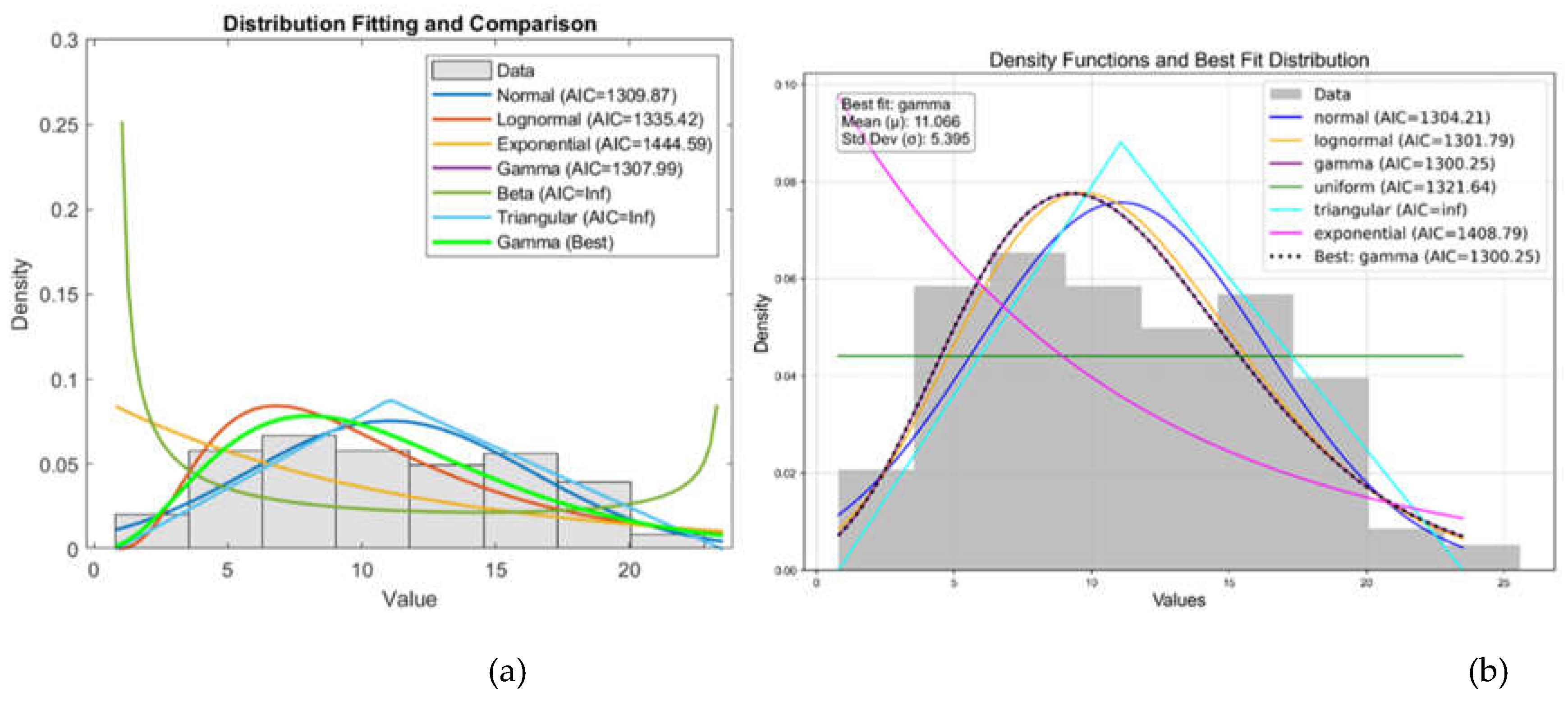
The left figure shows a Matlab result, while the right figure shows the same result calculated using Python code. The two plots show the results of a distribution fitting of a dataset, comparing several probability distributions based on the quality of the fit. In both plots, several distributions (normal, lognormal, gamma, uniform, triangular, and exponential) are fitted to the histogram of the data. The gamma distribution is the best fit, with the lowest AIC value. The gamma distribution closely follows the shape of the histogram, indicating a good fit. In both plots, AIC (Akaike Information Criterion) values were used to determine the fit: lower values indicate a better fit.
The MATLAB and Python code snippets both aim to identify the best-fitting statistical distribution based on the Akaike Information Criterion (AIC), yet exhibit notable differences. The MATLAB script employs a straightforward loop structure, normalizes data specifically for the Beta distribution without parameter constraints, computes log-likelihood directly from fitted distributions, and stores only the best-fitting model parameters and their AIC. In contrast, the Python implementation utilizes explicit normalization parameters (floc, fscale) for Beta distributions, separately manages the triangular distribution as a special case, computes additional statistics (mean, standard deviation) for each fit, systematically captures fitting errors via structured warnings, and returns comprehensive results for all distributions tested, including detailed statistical summaries. Overall, the Python approach provides greater analytical depth, explicit error handling, and enhanced result organization compared to the concise, more simplistic MATLAB methodology.
The essential parts of the codes have been highlighted below.
Matlab code for selecting best fit distribution:
% Fit each distribution and compute AIC
for i = 1:size(distributions, 1)
distName = distributions{i, 1};
distFunc = distributions{i, 2};
try
if strcmp(distName, 'Beta')
normalized_data = (data - min(data)) / (max(data) - min(data));
pd = distFunc(normalized_data);
else
pd = distFunc(data);
end
logL = sum(log(pdf(pd, data)));
k = length(pd.ParameterValues);
AIC = 2 * k - 2 * logL;
AIC_values(i) = AIC;
if AIC < bestAIC
bestAIC = AIC;
bestDist = distName;
bestParam = pd.ParameterValues;
bestPD = pd;
end
catch ME
fprintf('Error fitting %s distribution: %s\n', distName, ME.message);
end
end
Python code or selecting best fit distribution:
def fit_and_compare_distributions(data):
results = []
for name, dist in distributions.items():
try:
if name == "beta":
data_min, data_max = np.min(data), np.max(data)
normalized_data = (data - data_min) / (data_max - data_min)
params = dist.fit(normalized_data, floc=0, fscale=1)
ll = np.sum(dist.logpdf(normalized_data, *params))
mean, var = dist.stats(*params, moments="mv")
mean = mean * (data_max - data_min) + data_min
std = np.sqrt(var) * (data_max - data_min)
elif name == "triangular":
a, c = np.min(data), np.max(data)
b = np.mean(data)
loc = a
scale = c - a
params = ((b - a) / scale, loc, scale)
ll = np.sum(dist.logpdf(data, *params))
mean, var = dist.stats(*params, moments="mv")
std = np.sqrt(var)
else:
params = dist.fit(data)
ll = np.sum(dist.logpdf(data, *params))
mean, var = dist.stats(*params, moments="mv")
std = np.sqrt(var)
k = len(params)
aic = 2 * k - 2 * ll
results.append({
"distribution": name,
"params": params,
"log_likelihood": ll,
"aic": aic,
"mean": mean,
"std": std,
})
except Exception as e:
warnings.warn(f"Error fitting {name} distribution: {e}")
if results:
return results, min(results, key=lambda x: x["aic"])
else:
warnings.warn("No distributions successfully fitted to the data.")
return [], None
4. Statistical Analysis Results for Soil Physical and Strength Parameters
4.1. Correlation Analysis of Soil Physical Parameters
The three plots of the Figure 8 show the coefficient of determination (R2) values obtained for three different regression models for different soil types. Each plot shows the R2 values for three data treatment approaches: basic, dynamical filtering, and simple filtering. Higher R2 values indicate stronger model fit. Filtering methods, especially dynamical filtering, consistently produce higher R2 values for most soil types, suggesting that model performance improves when outliers are removed. High-plasticity clays and medium-plasticity clays generally yield the highest R2 values, especially in the dynamical filtered model, indicating that these soil types allow for more predictable relationships between the variables under study. In contrast, sandy silt (saSiS) and Silt (Si) show lower R2 values in the basic model, especially for the wet-dry bulk density relationship, suggesting greater data variability or nonlinear behavior in these soils. Predictive relationships between variables are significantly improved when filtering techniques are used. The choice of soil type plays a critical role in the strength of the regression model, with cohesive soils (e.g. clays) providing more reliable results. For practical applications of geotechnical modeling, data filtering is recommended to improve the robustness of regression-based predictions, especially for granular soils with higher natural variability.
Different data filtering methods produce different results, primarily because they remove outliers from the data set to different degrees. Basic filtering removes less data, resulting in more outliers entering the model and lower correlation (R2) values. Simple filtering removes outliers to a moderate extent, improving the model but retaining most of the data. On the other hand, dynamical filtering treats outliers iteratively and much more strictly, significantly increasing correlation values but causing a large amount of data loss. The result depends largely on the tested soil type and its natural variability. Cohesive soils, such as clays, have a lower natural variance, so more stringent filtering effectively improves the quality of the model while reducing the amount of data. In contrast, granular soils (e.g. sandy silts, sands) have greater natural variability, so overly strict filtering may result in the loss of a lot of data and lead to an overly simplified, idealized model. Results for each filtering method are shown in Figure 8, while the amount of data loss is presented in Table 2.
Table 2 presents the number of samples used in three different regression analyses—wet bulk density vs. void ratio, dry bulk density vs. void ratio, and wet bulk density vs. dry bulk density—across various soil types and data filtering approaches (basic, simple filtered, and dynamical filtered). For all soil types and relationships, a reduction in sample size is observed as data filtering is applied, particularly in the dynamical filtered approach. This indicates that outliers or influential data points have been systematically removed to improve model quality. Minimal sample loss is observed in fine-grained soils (e.g., clays), suggesting that these datasets contain fewer extreme outliers, whereas coarser soils (e.g., silty sand) show a more noticeable drop in sample size post-filtering. Data filtering significantly affects the available sample size, but it is necessary to enhance model accuracy, as supported by the higher R2 values observed in the filtered datasets.

Table 2.
Data loss during data filtering on Visonta samples.
| Soil type | Wet bulk density - void ratio | Dry bulk density - void ratio | Wet bulk density - dry bulk density | ||||||
|---|---|---|---|---|---|---|---|---|---|
| no. samples (basic) | no. samples (simple filtered) | no. samples (dynamical filtered) | no. samples (basic) | no. samples (simple filtered) | no. samples (dynamical filtered) | no. samples (basic) | no. samples (simple filtered) | no. samples (dynamical filtered) | |
| Sand (Sa) | 60 | 58 | 56 | 59 | 57 | 28 | 59 | 57 | 56 |
| sandy Silt (saSi) | 206 | 197 | 164 | 206 | 197 | 159 | 206 | 196 | 195 |
| Silt (Si) | 67 | 64 | 63 | 67 | 65 | 56 | 67 | 65 | 64 |
| silty Sand (siSa) | 113 | 107 | 99 | 113 | 108 | 91 | 113 | 105 | 100 |
| high plasticity Clay | 429 | 413 | 396 | 428 | 414 | 374 | 428 | 421 | 396 |
| medium plasticity Clay | 189 | 186 | 175 | 188 | 185 | 179 | 188 | 186 | 176 |
| low plasticity Clay | 68 | 64 | 65 | 68 | 64 | 59 | 68 | 62 | 61 |
Clays, especially those with high plasticity, are more stable in terms of data quality, making them preferable for regression-based modeling. Granular soils, due to their higher natural variability, may require more aggressive filtering and careful interpretation to ensure reliable predictions. Thus, the filtering process is justified despite the reduction in sample size, as it contributes to more statistically sound models. The dynamical filtering overestimates the true correlation. Where many values have been filtered out, the difference between the R2 values in the diagram is more significant.
4.1.1. Wet density –void ratio
Figure 9 illustrates the relationship between wet bulk density (horizontal axis) and void ratio (vertical axis) for various soil types, each represented by a distinct color. A negative correlation is clearly observed: as wet bulk density increases, the void ratio decreases. Denser soils typically contain less pore space. The distribution of data points suggests that the strength of this relationship varies among soil types. Clayey soils (e.g., high plasticity clay, clayey sand) are associated with higher void ratios at lower wet bulk densities, showing greater variability and a wider spread. The low wet bulk density values for the high plasticity clays are related to high organic content, since the organic content reduces the density of the clays. Some clay layers contain different amounts of organic materials. Sands and silts (e.g., sand, sandy silt, silty sand) are clustered at higher densities and lower void ratios, indicating more compacted and less compressible structures. A few outliers can be identified, particularly among clayey sands, suggesting that some variability remains unexplained and may be due to heterogeneity in sample properties or measurement inconsistencies.
4.1.2. Dry density – void ratio
Figure 10 displays the relationship between dry bulk density (horizontal axis) and void ratio (vertical axis) for a variety of soil types, each indicated by a different color. A clear inverse relationship is observed: as dry bulk density increases, the void ratio decreases. This trend is consistent with fundamental soil mechanics, where denser soils contain less void space. The data points corresponding to high plasticity clays show a wider spread and are concentrated toward lower dry bulk densities and higher void ratios, indicating a more porous and compressible structure. In contrast, granular soils (e.g., sand, silty sand) are distributed toward the higher density–lower void ratio region, reflecting more compacted conditions with less variability. The tight clustering of points for medium plasticity clays and sands suggests more consistent behavior and potentially better predictability in modeling efforts. A few outliers are present, primarily among clay-rich soils, suggesting heterogeneity in sample characteristics or testing conditions. Low dry bulk density values indicate organic matter content. The higher the organic matter content, the lower the dry bulk density as it is mentioned above.
4.1.3. Wet bulk density – dry bulk density
Figure 11 displays the relationship between dry bulk density (x-axis) and wet bulk density (y-axis) for various soil types, each marked with a different color. A strong positive linear relationship is observed: as dry bulk density increases, wet bulk density also increases. This aligns with expectations, as wet bulk density includes both the solid particles and the water content, while dry bulk density considers only the solids. Most soil types follow this linear trend closely, particularly sands, silts, and clays with medium or low plasticity, indicating a consistent relationship across a wide range of soils. High plasticity clays are more widely spread and appear at lower dry bulk densities with correspondingly lower wet bulk densities. This suggests greater variability in water content and structure, which is typical of such fine-grained, compressible soils. The reason for that is the high organic content of some of the high plasticity clay samples, as mentioned before. The tight clustering of sands and silts near the trend line indicates more predictable and uniform behavior. The relationship between dry and wet bulk densities can be reliably modeled with a linear regression, particularly for non-cohesive and low-plasticity soils.
4.1.4. Plasticity Index – Liquid Limit
Figure 12 shows the relationship between the liquid limit and the plasticity index for different soil samples. A reference line—Line A, defined by the equation Ip=0.73(wL-20) —is also included to assist in classification, following the widely used Casagrande plasticity chart method. A positive correlation is clearly observed: as the liquid limit increases, the plasticity index also increases, indicating that soils with higher water content at the liquid limit tend to have greater plasticity ranges. The data points are color-coded by soil type, with dark red points representing high plasticity clays, while cyclamen, grey and green points representing lower-plasticity silts and clays. Most of the points lie around the A-line, except some of the high plasticity clays, mainly with very high liquid limit. Based on the analysis of the Casagrande diagram, it can be determined that some of the high plasticity clays are located below the A-line, which typically indicates an increased organic matter content of the samples.
4.1. Statistical Analysis of Shear Strength Parameters
The boxplot on Figure 13 presents the distribution of friction angle (φ) values for the investigated soil types, providing insight into their shear strength characteristics. Sands (Sa), sandy silts (saSi), and silty sands (siSa) show relatively higher median φ values, generally ranging between 25° and 30°, with some values extending above 35°.
This is expected, as granular soils typically exhibit higher friction angles. Silts (Si) and clays (high, medium, and low plasticity) demonstrate lower φ values, with medians between 10° and 25°, indicating more compressible, less frictional behavior. High plasticity clays have the lowest median and minimum φ values. Variation is higher among fine-grained soils, particularly clays, as seen from the larger interquartile ranges and whiskers, implying greater heterogeneity. These findings highlight the importance of soil classification and testing for proper geotechnical evaluation and design safety.
The boxplot on Figure 14 illustrates the cohesion values (in kPa) for the investigated soil types. It can be observed that sands (Sa), sandy silts (saSi), silts (Si), and silty sands (siSa) exhibit relatively low cohesion values. In contrast, clays, particularly those with high and medium plasticity, demonstrate significantly higher cohesion, with values extending beyond 200 kPa in some cases. Low plasticity clay also shows moderately high cohesion, though with a wider variability. These results indicate that cohesion is strongly influenced by the soil's plasticity and composition.
5. Application of the Statistical Analyses of the Investigated Soils for Probabilistic Slope Stability Calculations
5.1. Input Data
5.1.1. Characteristic Soil Properties
The investigatory drillings determined the stratum of the investigated area. Sections for the calculations were determined according to the determined layers. Example sections can be seen in Figure 4. Based on the laboratory results, the characteristic properties (unit weight, cohesion and angle of friction) were determined for each layer, which are in Table 3. The characteristic values were used for deterministic stability calculations and for some layers in the probabilistic stability calculations, where not enough data was available for the probabilistic approach.
5.1.2. Probabilistic Soil Properties
On Figure 15 the best-fitting statistical distributions for unit weight of various soil types can be seen, determined using multiple methods: CumFreq (MAE), EasyFit (Kolmogorov–Smirnov, Anderson–Darling, Chi-Squared), and Akaike Information Criterion (AIC) via Matlab and Python. Lognormal, Normal, Gamma, and Beta distributions are predominantly identified. Lognormal and Normal distributions are frequently favored, especially by MAE and AIC-based evaluations. For example, low plasticity clay and silty sand are consistently best described by the Lognormal distribution across most methods. Beta distributions are commonly associated with high plasticity clays. Table 4 show the results of the probabilistic analyses.
Figure 16 summarizes the best-fit probability distributions for shear strength parameters of the investigated soil types, using several goodness-of-fit methods: CumFreq (MAE), EasyFit (Kolmogorov–Smirnov, Anderson–Darling, Chi-Squared), and Akaike Information Criterion (AIC) applied via Matlab and Python. Gamma and Normal distributions are most frequently selected, particularly for clay soils. Uniform and Triangular distributions are more often associated with sandy and silty soils, especially in EasyFit methods. Lognormal and Exponential distributions are mainly linked to Silt and Silty Sand for phi, especially in AIC-based evaluations. Table 5 and 6 show the results of the analysis for the cohesion and angle of friction.
5.2. Results of the Slope Stability Analysis
The introduced statistical data processing were used in practice to determine the stability of the slopes of the open pit lignite mine. Both deterministic and probabilistic slope stability calculations were done using the Slide2 software on the 7 sections, which are shown in Figure 1. The results demonstrate the difference between the two methods and the importance of the probabilistic approach.
5.2.1. Deterministic Calculation Results
The results of the deterministic analysis are encouraging, the slope proved to be stable for all sections. Due to the minimum safety factor of 1.35, slope optimization was later performed on Section 3, Section 4 and Section 7, but this is not discussed in this study.
Table 7.
Deterministic test results of all Sections.
| Section 1 | Section 2 | Section 3 | Section 4 | Section 5 | Section 6 | Section 7 | |
|---|---|---|---|---|---|---|---|
| FS [-] | 1.951 | 1.379 | 1.305 | 1.226 | 1.653 | 1.583 | 1.334 |
Figure 17 shows the deterministic calculation result of the Section 1. The Factor of Safety (FS=1.951) is above the desired value, the slope is stable according to the result.
5.1.2. Probabilistic Calculation Results
Table 8 presents the results of the probabilistic slope stability study of the Visonta Keleti-III lignite mine. The FS (Factor of Safety), PF (Probability of Failure), and RI (Reliability Index) values in the table were determined for the different sections based on the Bishop simplified method and Latin Hypercube simulation. Latin Hypercube analysis is an advanced version of Latin Hypercube simulation that samples the entire set of input parameter values in a structured manner, thus increasing the efficiency and accuracy of the simulation. FS is the result of a deterministic calculation run with the Mean values of the parameters. FS (mean) is the expected FS value obtained from the results of 1000 runs, where the Mean value takes on a different value in each run. Based on the FS values, Section 3 (FS = 2,060) is the most stable section, while Section 2 (FS = 1,207) is the most critical. In terms of PF, i.e. the probability of failure, Section 2 is particularly risky, as it shows a 46.7% failure probability. The results of the research confirm that traditional deterministic models cannot reliably handle the spatial uncertainty of geotechnical parameters in the Visonta mine area. The probabilistic approach using Latin Hypercube simulation provides a more detailed and realistic assessment of slope stability, which is essential for safe mine design.
After the statistical analysis was completed and the statistical parameters were obtained, the practical implementation followed. In addition to the statistical parameters, there was a need for characteristic values. The Visonta mining area was very densely stratified, as shown in the Figure 4, so for several layers there were only characteristic input data. For the rest, we calculated with probabilistic values. The interpretation of the results of the probabilistic slope stability calculation is presented on Section 1 of the Visonta mining area. Figure 18 displays a probabilistic analysis of slope stability of this section using the Bishop simplified method.
Figure 19 shows a histogram of the Factor of Safety (FS) with relative frequency on the y-axis.The distribution is right-skewed, indicating a larger concentration of simulations resulting in FS values between approximately 1.3 and 1.7, with a peak near 1.5.The orange bars on the left (FS < 1.0) represent failure cases, where the slope is not considered stable. The blue bars correspond to stable conditions (FS ≥ 1.0). A fitted probability density function (PDF) curve is overlaid in grey, approximating the distribution trend.
The results indicate that while the majority of simulations show a stable slope, a non-negligible probability of failure exists. This probabilistic approach highlights the variability and uncertainty in slope stability due to input parameter distributions.
Figure 20 illustrates the Cumulative Distribution Function (CDF) of the Factor of Safety (FS) calculated using the Bishop simplified method. The x-axis represents the Factor of Safety, and the y-axis shows the corresponding cumulative probability. The curve exhibits a typical sigmoidal shape, characteristic of cumulative distributions. At FS = 1.0, the cumulative probability is approximately 0.11, indicating a 11% probability of failure.
The graph in Figure 21 illustrates the convergence behavior of the Probability of Failure (PF) calculated via the Bishop simplified method as a function of the number of Latin Hypercube samples. The x-axis represents the number of samples, while the y-axis shows the corresponding PF (%). Initial estimates (<100 samples) show high variability and instability, as expected with low sample sizes. Around 200–300 samples, the PF begins to stabilize, with fluctuations decreasing progressively. From approximately 600 samples onwards, the PF converges around 11–12%, indicating statistical stability of the estimated probability of failure. This behavior confirms that at least several hundred samples are required for reliable PF estimation in slope stability analysis using probabilistic methods. This plot is essential for validating the adequacy of amount of samples in probabilistic geotechnical modeling.
6. Discussion
The probability of failure (PF) results from the probabilistic stability study conducted in the Keleti III part of the Visonta mining area highlight the risk assessment limitations of traditional deterministic methods and confirm the need for a probabilistic approach. The effectiveness of probabilistic slope stability studies is also supported by other research, especially studies using metaheuristic methods, such as Zeng et al. [52], where hybrid optimization algorithms were used to assess slope safety more reliably. The spatial variability of physical soil parameters fundamentally affects the reliability of slope stability studies. Therefore, probabilistic analyses complementing deterministic approaches are necessary for safe planning.
The acceptability of failure probability is a widely discussed issue. There is no agreed consensus, only recommendations and tables [10][16-28]. Numerous interpretations of PF are apparent after reviewing several articles related to PSSA from the past decades. In their article, Ng and Kok Shein [29] considered a value below 5% safe, while above 25% they considered it a high risk. Penalba et al. [30] in their work considered a 6% failure probability acceptable. Bi et al. [31] is quite permissive, stating that slopes below 50% are safe. Moradi et al. [32] maximized the allowable failure probability at 5%. In their case study in Taiwan, Wang et al. [33] considered the failure probability of 17.3% to be too high. Hamedifar et al. [34] considered 30% to be dangerous. According to Kulatilake et al. [35], 5% is the permissible limit, and Chaulagai [36] had the same opinion. Mandal et al. [37] said that the slope was not considered safe for a PF=15%. Nerman et al. [38] in 2018 set a PF value of 10% as the upper limit. However, Obregon [39] determined the maximum at 20%. Sitharam [40] quotes Sjöberg [41], meaning that the PF obtained of 7.5% is acceptable, but close to the 10% limit. Rafiei [42] claimed that PF should be below 10-15%. Mathe & Ferentinou [43] and Sachpazis [44] capped the maximum allowable value of PF at 5% . Sdvyzhkova et al. [45] assessed a PF value of 12.55% as a significant slip hazard. Do et al. [46] recommend a 10-20% allowable PF. However, Li et al. [47] wrote that a PF greater than 5-10% is no longer acceptable. Nguyen et al.'s [48] is even more stringent, according to their results, PF=2.2% cannot be considered safe. Abhijith et al. [49] interpret a PF greater than 17% as a potential danger zone, and this was based on the recommendation of the US Army Corps of Engineers (1997) [50].
These studies show no final consistent agreement on the maximum value of PF. It is important to keep in mind Ferreira's [51] statement, after Wesseloo & Read (2009) [21], that the minimum FS and maximum PF requirements must be evaluated simultaneously.
The calculated FS and PF of the slope of the Visonta lignite mine also show that it is not easy to evaluate the long-term stability according to the results. When the FS was around 1.50, which was considered stable, the PF was between 0 - 11%, which can be stable but bigger than the 5% limit, which was considered the upper limit of the safe zone in some of the above-mentioned studies. When the SF was 1.33 at section 7, then the PF was 0%, so it can be considered stable.
For a more exact evaluation of the PF results, it should take into account the consequence of a failure as well as it is determined by Gibson [10] and Adams [23]. When a failure can cause serious problems, damages in valuables or endanger human life then the limit of the PF should be small, other case it could be bigger. In this case study according to Adams [23] the accepted risk can be moderate so the upper limit of the PS should be 10%
7. Conclusions
The paper presents a comprehensive probabilistic geotechnical study of the Visonta Keleti-III lignite mining area in Hungary, emphasizing the statistical evaluation of soil parameters and their integration into probabilistic slope stability analysis. The Visonta mine is situated in a geologically complex basin with Pliocene lignite seams overlain by Quaternary sediments. Thirteen distinct soil types were classified based on plasticity index and grain size distribution, including various clays, silts, sands, and their mixtures. The deposit is stratified, with considerable heterogeneity in layer composition, thickness, and geotechnical behavior. Over 3,300 lab samples from 28 boreholes were processed using a multi-phase outlier filtering method (manual, IQR-based, and dynamical filtering via Python), improving model fit and regression robustness. Relationships between parameters like bulk densities, void ratio, and plasticity were modeled with strong correlation, especially in cohesive soils. Best-fit distributions for unit weight and shear strength parameters (φ and c) were identified using various tools (CumFreq, EasyFit, Matlab, Python). Gamma, Normal, and Lognormal distributions were most frequently selected, with variability across soil types and parameters. The Bishop simplified method combined with Latin Hypercube simulation was employed. A histogram of FS showed a right-skewed distribution, with most results between 1.3–1.7, but with ~20% probability of failure (FS < 1.0). The CDF plot validated this, and the PF convergence plot indicated stability after ~600 simulations, suggesting adequacy of the sample size. This study demonstrates the necessity and effectiveness of probabilistic approaches in slope stability evaluation within a mining context. Traditional deterministic models often overlook the spatial and statistical variability of soil properties, leading to potential underestimation or overestimation of slope safety. The integration of advanced filtering techniques, tailored distribution fitting, and Latin Hypercube simulation allows for realistic modeling of geotechnical behavior. Importantly, the application of such methods highlights the value of data quality and parameter uncertainty, especially in stratified and variable geological formations like Visonta. The use of custom Python and Matlab tools optimized for compatibility with engineering software (e.g., Rocscience) presents a practical contribution to geotechnical data processing and modeling workflows. The probabilistic method outperforms traditional approaches by quantifying uncertainty and providing realistic estimates of failure probability. Cohesive soils, particularly clays, showed more predictable relationships and better model fit after filtering. The estimated 11–12% probability of failure in section 1 indicates that while the slope is mostly stable, design mitigation may be warranted. Tools and techniques developed (e.g., Python filtering and distribution fitting) provide a reproducible, scalable workflow for similar geotechnical investigations.
Author Contributions
Conceptualization, Petra Oláh and Péter Görög; Formal analysis, Petra Oláh and Péter Görög; Funding acquisition, Péter Görög; Investigation, Petra Oláh and Péter Görög; Methodology, Petra Oláh; Project administration, Péter Görög; Software, Petra Oláh and Péter Görög; Supervision, Péter Görög; Validation, Petra Oláh and Péter Görög; Writing – original draft, Petra Oláh; Writing – review & editing, Péter Görög. All authors have read and agreed to the published version of the manuscript.
Data Availability Statement
The data presented in this study are available on request from the corresponding authors. The data is not publicly available due to data confidentiality.
Acknowledgments
The support provided by the Ministry of Culture and Innovation of Hungary from the National Research, Development and Innovation Fund, financed under the TKP2021-NVA funding scheme (project no. TKP-6-6/PALY-2021). The home institutions of the authors provided technical and administrative support. Furthermore, this research is supported by the MVM Matra Energy Ltd. The authors are deeply grateful for this support.
Conflicts of Interest
The authors declare no conflict of interest. The funders had no role in the design of the study; in the collection, analyses, or interpretation of data; in the writing of the manuscript, or in the decision to publish the results.
References
- Duncan, J. M., & Wright, S. G. (2005). Soil Strength and Slope Stability. John Wiley & Sons.
- Harr, M. E. (1987). Reliability-Based Design in Civil Engineering. McGraw-Hill.
- Fenton, G. A., & Griffiths, D. V. (2008). Risk Assessment in Geotechnical Engineering. John Wiley & Sons.
- Griffiths, D. V., & Lane, P. A. (1999). Slope stability analysis by finite elements. Geotechnique, 49(3), 387-403.
- Selby, M. J. (1993). Hillslope Materials and Processes. Oxford University Press.
- Bate, B., & McMahon, B. T. (2017). Numerical analysis of anisotropy in geotechnical engineering. Journal of Geotechnical Research, 12(2), 45-60.
- Christian, J. T., & Baecher, G. B. (2003). Probabilistic analysis in geotechnical engineering. Journal of Geotechnical and Geoenvironmental Engineering, 129(4), 307-317.
- Hammah, R., Yacoub, T. and Curran, J. (2009). Probabilistic Slope Analysis with the Finite Element Method. Proc. 43rd US Symp. on Rock Mechanics & 4th US-Canada Rock Mechanics Symp., Asheville.
- Chiwaye, Henry & Stacey, T.R.. (2010). A comparison of limit equilibrium and numerical modelling approaches to risk analysis for open pit mining. Journal of the Southern African Institute of Mining and Metallurgy. 110. 571-580.
- Gibson, William. (2011). Probabilistic Methods for Slope Analysis and Design. Australian Geomechanics Journal. 46. 29. 46(3):1–11.
- Chuaiwate, P.; Jaritngam, S.; Panedpojaman, P.; Konkong, N. Probabilistic Analysis of Slope against Uncertain Soil Parameters. Sustainability 2022, 14, 14530. [CrossRef]
- He, Y., Li, Z., Wang, W. et al. Slope stability analysis considering the strength anisotropy of c-φ soil. Sci Rep 12, 18372 (2022). [CrossRef]
- Teng L, He Y, Wang Y, Sun C and Yan J (2024) Numerical stability assessment of a mining slope using the synthetic rock mass modeling approach and strength reduction technique. Front. Earth Sci. 12:1438277. [CrossRef]
- Horváth, Zoltán & Micheli, Erika & Mindszenty, A. & Berényi Üveges, Judit. (2005). Soft-sediment deformation structures in Late Miocene–Pleistocene sediments on the pediment of the Mátra Hills (Visonta, Atkár, Verseg): Cryoturbation, load structures or seismites?. Tectonophysics. 410. 81–95. [CrossRef]
- Erdei, B. & Hably, L. & Selmeczi, I. & Kordos, L. (2011). Palaeogene and Neogene localities in the North-Hungarian Mountain Range. Guide to the post-congress fieldtrip of the 8th EPPC, 2010, Budapest, Hungary. Studia Botanica Hungarica. 42. 153-183.
- Priest S. D., Brown E. T. Probabilistic stability analysis of variable rock slopes. Transactions of Institution of Mining and Metallurgy. Section A: Mining Industry. 1983. Vol. 92. pp. A1 A12.
- Pine RJ (1992) Risk analysis design application in mining geomechanics, transactions of institute of mining and metallurgy, (Section A: Mining Industry), pp A149–A158.
- Sullivan, T. 2006. Pit slope design and riskA view of the current state of the art. In Proceeding of International Symposium on Stability of Rock Slopes in Open Pit Mining and Civil Engineering Situations.
- Silva, F., Lambe, T. W., & Marr, W. A. (2008). Probability and risk of slope failure. Journal of Geotechnical and Geoenvironmental Engineering, 134(12), 1691–1699. [CrossRef]
- Read, J., and Stacey, P. 2009. Guidelines for open-pit slope design. Collingwood, CSIRO, Australia.
- Wesseloo J, Read J (2009) Chapter 9 - acceptance criteria. In: Read J, Stacey P (eds) Guidelines for open pit slope design. CIRSO publishing, Clayton, pp 221–236.
- Hormazabal, E., Tapia, M., Fuenzalida, R., and Zuniga, G. 2011. Slope optimization for the Hypogene Project at Carmen de Andacollo Pit, Chile. In Proceedings of Slope Stability 2011, International Symposium on Rock Slope Stability in Open Pit Mining and Civil Engineering, Vancouver, B.C., Canada.
- Adams, Brian. (2015). Slope Stability Acceptance Criteria for Opencast Mine Design.
- Hawley, M., & Cunning, J. (2017). Guidelines for mine waste dump and stockpile design. CRC Press.
- 25. Chakraborty, Rubi & Dey, Arindam. (2022). Probabilistic Slope Stability Analysis: State-of-the-Art Review and Future Prospects. Innovative Infrastructure Solutions. 7. 1-19. [CrossRef]
- Che, Wei & Chang, Pengfei & Wang, Wenhao. (2023). Optimal Intensity Measures for Probabilistic Seismic Stability Assessment of Large Open-Pit Mine Slopes under Different Mining Depths. Shock and Vibration. 2023. 1-23. [CrossRef]
- Idris, Musa & A.S, Kolade. (2024). Probabilistic Slope Stability Assessment For Sustainable Mining At Ankpa Coal Mine, Nigeria. Futa Journal Of Engineering And Engineering Technology. 18. 93 - 100.
- Ferreira Filho, Flávio & Bacellar, Luis & Marques, Eduardo Antonio & Assis, Andre & Gomes, Romero & Costa, Teófilo. (2025). Failure Susceptibility Analysis of Open Pit Slopes: A Case Study from the Quadrilátero Ferrífero Mine, Brazil. Geotechnical and Geological Engineering. 43. [CrossRef]
- Ng, Kok Shien. (2005). Reliability analysis on the stability of slope.
- Peñalba, R. F., Luo, Z., & Juang, C. H. (2009). Framework for probabilistic assessment of landslide: A case study of El Berrinche. Environmental Earth Sciences, 59(3), 489-499. https://doi.org/10.1007/s12665-009-0046-0.
- Bi, R., Ehret, D., Xiang, W. et al. Landslide reliability analysis based on transfer coefficient method: A case study from Three Gorges Reservoir. J. Earth Sci. 23, 187–198 (2012). [CrossRef]
- Moradi, Ali & Morteza, Osanloo. (2014). Determination and stability analysis of ultimate open-pit slope under geomechanical uncertainty. International Journal of Mining Science and Technology. 24. [CrossRef]
- Wang, Lei & Hwang, Jin-Hung & Luo, Zhe & Juang, C.Hsein & Xiao, Junhua. (2013). Probabilistic back analysis of slope failure – A case study in Taiwan. Computers and Geotechnics. 51. 12–23. [CrossRef]
- Hamedifar, Hamed & Bea, Robert & Pestana, Juan & Roe, Emery. (2014). Role of Probabilistic Methods in Sustainable Geotechnical Slope Stability Analysis. Procedia Earth and Planetary Science. 9. 132–142. [CrossRef]
- Kulatilake, Pinnaduwa & Shu, Biao & Sherizadeh, Taghi & Jh, Deng. (2014). Probabilistic block theory analysis for a rock slope at an open pit mine in USA. Computers and Geotechnics. 61. 254–265. [CrossRef]
- Chaulagai, Rabindra & Osouli, Abdolreza & Clemente, Jose. (2017). Probabilistic Slope Stability Analyses - A Case Study. 444-452. [CrossRef]
- Mandal, Jagriti & Narwal, Sruti & Gupte, Dr. (2017). Back Analysis of Failed Slopes - A Case Study. International Journal of Engineering Research and. V6. 10.17577/IJERTV6IS050366. Preprints.org (www.preprints.org) | NOT PEER-REVIEWED | Posted: 6 May 2025. [CrossRef]
- Neman, N & Zakaria, Zufialdi & Sophian, Irvan & Adriansyah, Yan. (2018). Probability of Failure and Slope Safety Factors Based on Geological Structure of Plane failure on Open Pit Batu Hijau Nusa Tenggara Barat. IOP Conference Series: Earth and Environmental Science. 145. 012077. [CrossRef]
- Obregon, Christian & Mitri, Hani. (2019). Probabilistic approach for open pit bench slope stability analysis – A mine case study. International Journal of Mining Science and Technology. 29. [CrossRef]
- Sitharam T.G. & Amarnath M. Hegde, 2019. "A Case Study of Probabilistic Seismic Slope Stability Analysis of Rock Fill Tailing Dam," International Journal of Geotechnical Earthquake Engineering (IJGEE), IGI Global, vol. 10(1), pages 43-60, January.
- Sjöberg, J. (1999). Analysis of large scale rock slopes (PhD dissertation, Luleå tekniska universitet). Retrieved from https://urn.kb.se/resolve?urn=urn:nbn:se:ltu:diva-18773.
- Rafiei Renani, Hossein & Martin, Derek & Varona, Pedro & Lorig, Loren. (2019). Stability Analysis of Slopes with Spatially Variable Strength Properties. Rock Mechanics and Rock Engineering. 52. 1-18. [CrossRef]
- Mathe, Lewis & Ferentinou, Maria. (2021). Rock slope stability analysis adopting Eurocode 7, a limit state design approach for an open pit. IOP Conference Series: Earth and Environmental Science. 833. 012201. [CrossRef]
- Sachpazis, D.C. (2019, October 06). Probabilistic Slope Stability Evaluation. In Encyclopedia. https://encyclopedia.pub/entry/116.
- Sdvyzhkova, Olena & Moldabayev, Serik & Bascetin, Atac & Babets, Dmytro & Kuldeyev, Erzhan & Sultanbekova, Zhanat & Amankulov, Maxat & Issakov, Bakhytzhan. (2022). Probabilistic assessment of slope stability at ore mining with steep layers in deep open pits. Mining of Mineral Deposits. 16. 11-18. Do et al. [CrossRef]
- Do, Van & The, Viet & Tran, The Viet & Nguyen, Ha & Pham, Huy & Nguyen, Van. (2023). Integrating Soil Property Variability In Sensitivity And Probabilistic Analysis Of Unsaturated Slope: A Case Study. International Journal of GEOMATE. 25. 132-139.However, in the 2024 article by Li et al.
- Li, Tianzheng & Gong, Wenping & Zhu, Chun & Tang, Huiming. (2024). Stability evaluation of gentle slopes in spatially variable soils using discretized limit analysis method: a probabilistic study. Acta Geotechnica. 19. 6319-6335. Nguyen et al.'s. [CrossRef]
- Nguyen, Phu Minh Vuong & Marciniak, Michał. (2024). Stochastic Rock Slope Stability Analysis: Open Pit Case Study with Adjacent Block Caving. Geotechnical and Geological Engineering. 42. 5827-5845. 10.1007/s10706-024-02862-w. In their 2024 article, Abhijith et al.
- A., Abhijith & Pillai, Rakesh. (2024). TRIGRS-FOSM: probabilistic slope stability tool for rainfall-induced landslide susceptibility assessment. Natural Hazards. 121. 3401-3430. [CrossRef]
- US Army Corps of Engineers (1997) Engineering and design: introduction to probability and reliability methods for use in geotechnical engineering. Engineer Technical Letter 1110-2-547. Washington, DC: Department of the Army.
- Ferreira Filho, Flávio & Bacellar, Luis & Marques, Eduardo Antonio & Assis, Andre & Gomes, Romero & Costa, Teófilo. (2025). Failure Susceptibility Analysis of Open Pit Slopes: A Case Study from the Quadrilátero Ferrífero Mine, Brazil. Geotechnical and Geological Engineering. 43. [CrossRef]
- Zeng, X., Khajehzadeh, M., Iraji, A., Keawsawasvong, S. “Probabilistic Slope Stability Evaluation Using Hybrid Metaheuristic Approach”, Periodica Polytechnica Civil Engineering, 66(4), pp. 1309–1322, 2022. [CrossRef]
Figure 1.
(a) Hungary in Europe. (b) Visonta lignite site in Hungary. (c) Location and sections of Keleti-III Lignite Mine, in Visonta.
Figure 1.
(a) Hungary in Europe. (b) Visonta lignite site in Hungary. (c) Location and sections of Keleti-III Lignite Mine, in Visonta.
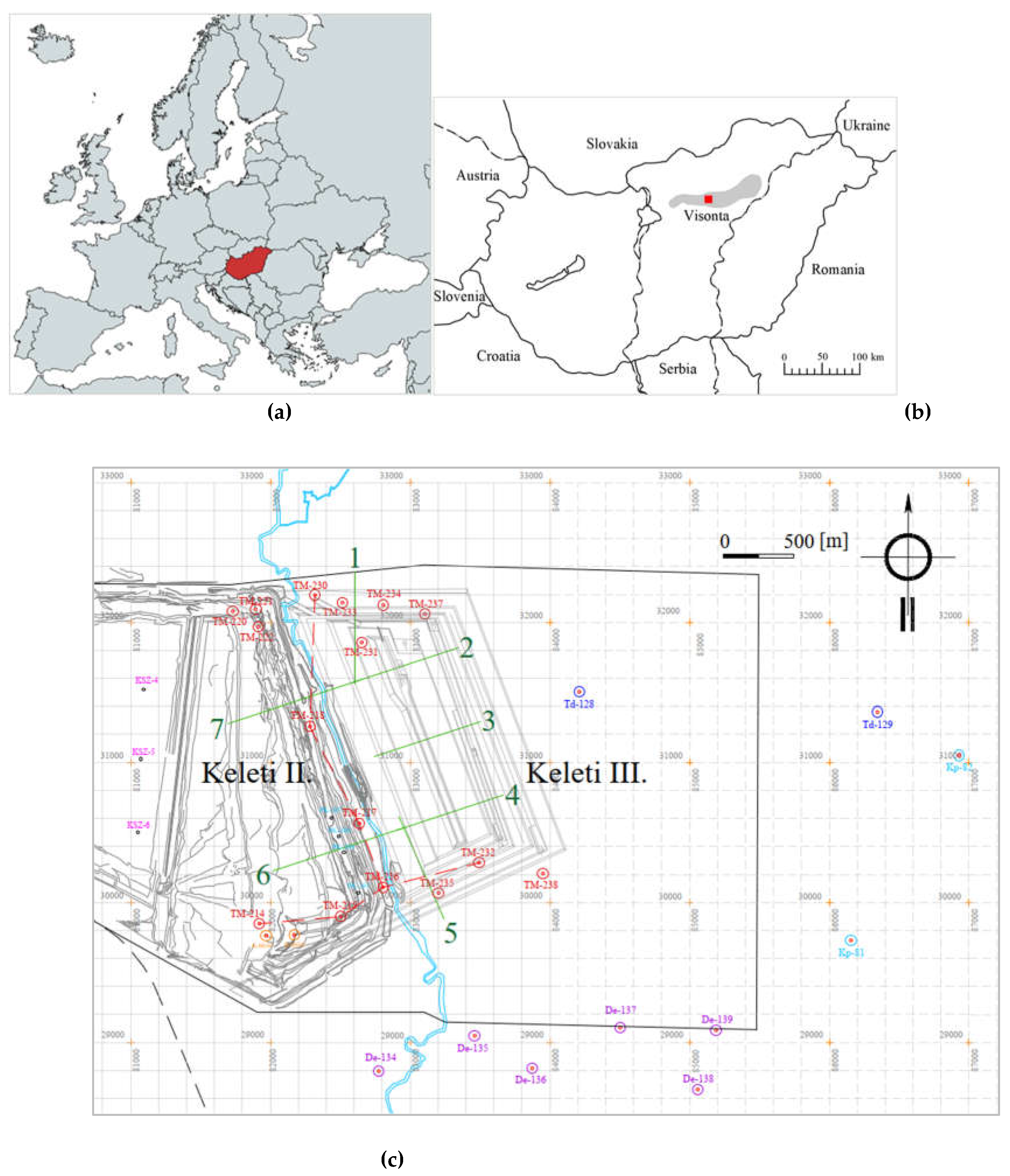
Figure 3.
Geological structure of the Keleti-I mine (simplified, schematic stratigraphy) [14].
Figure 3.
Geological structure of the Keleti-I mine (simplified, schematic stratigraphy) [14].
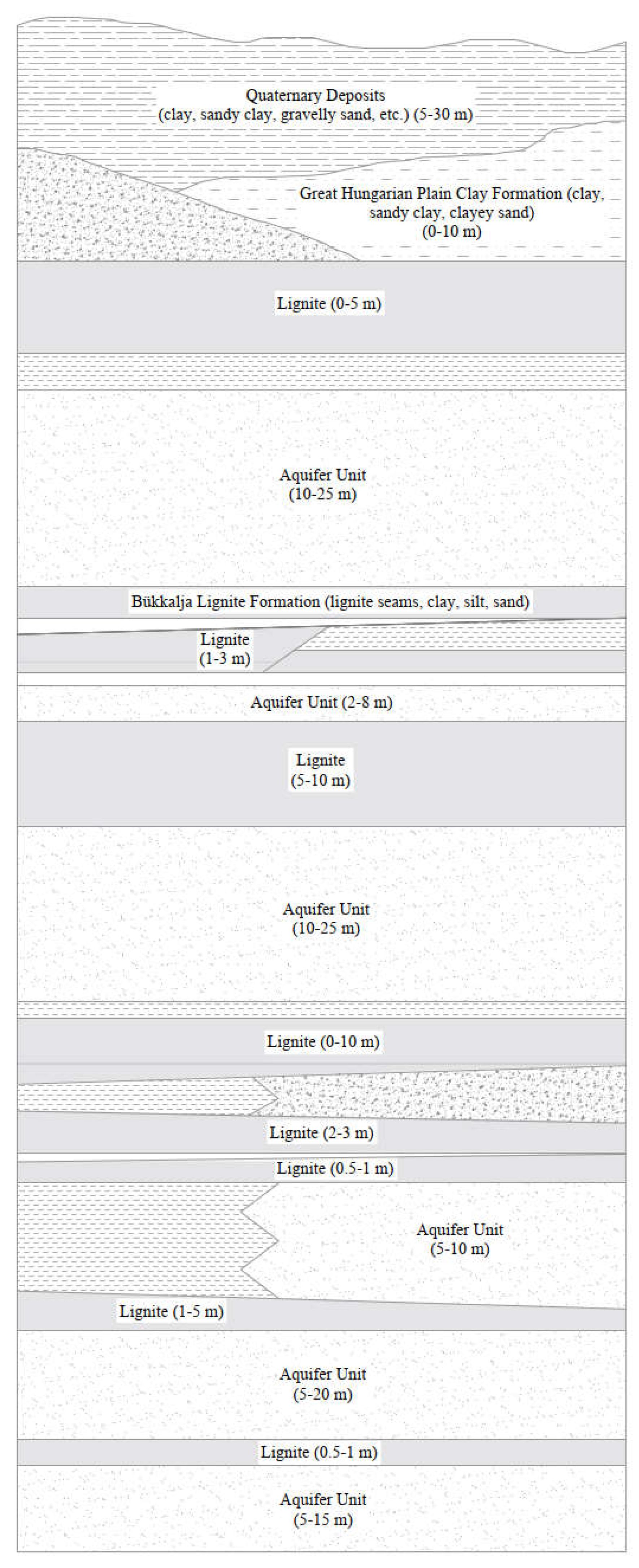
Figure 4.
Geotechnical Cross-Sections of the Visonta Keleti-III Mining Area.
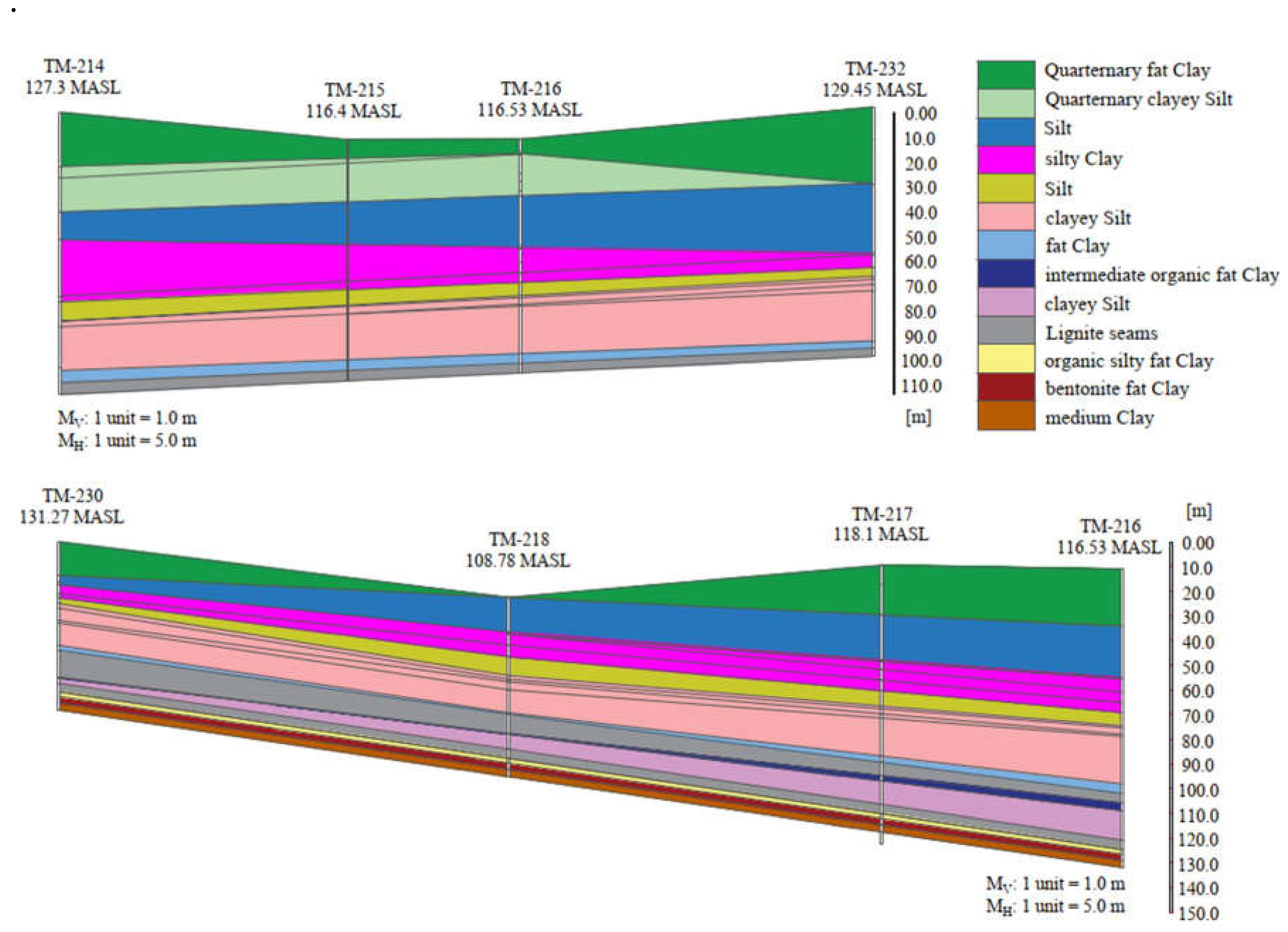
Figure 5.
Workflow of Soil Classification and Probabilistic Slope Stability Analysis in the Visonta Mining Area.
Figure 5.
Workflow of Soil Classification and Probabilistic Slope Stability Analysis in the Visonta Mining Area.
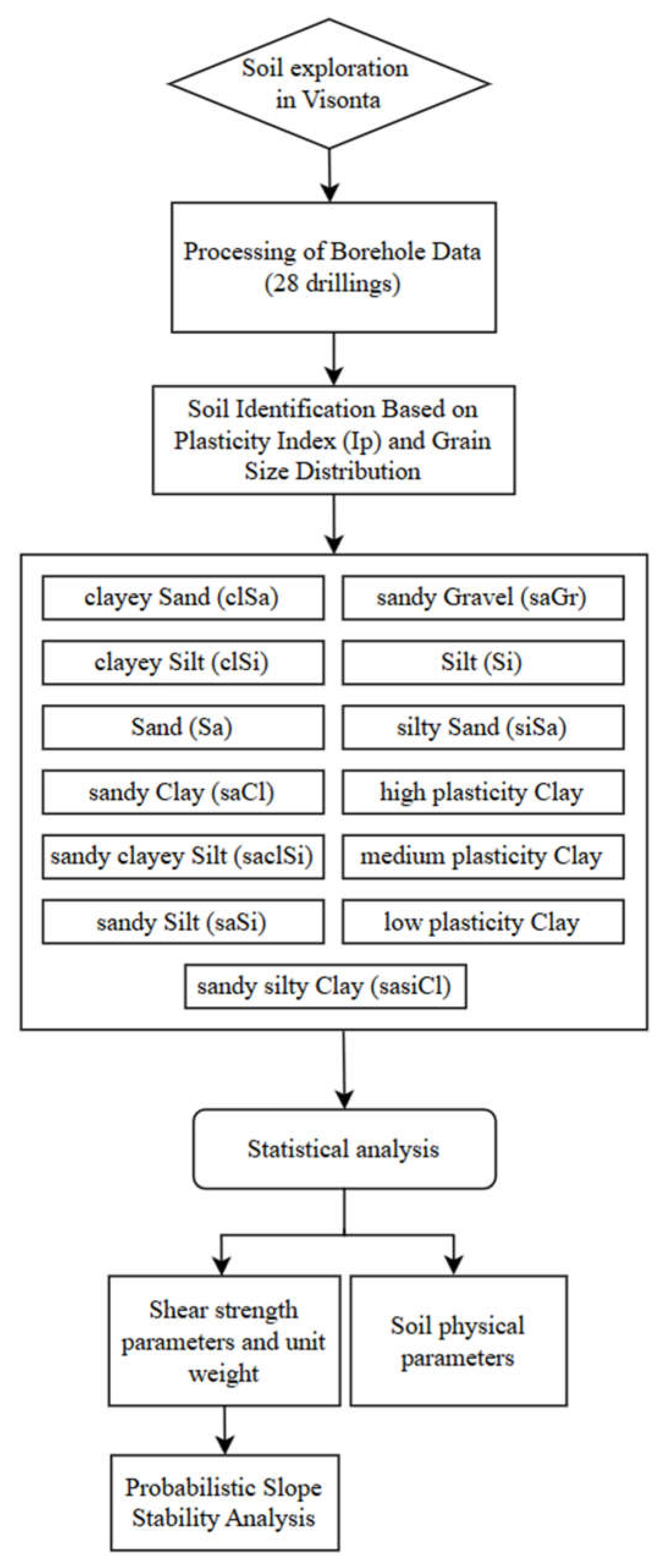
Figure 8.
(a) Correlation analysis of wet bulk density – void ratio (b) Correlation analysis of dry bulk density - void ratio (c) Correlation analysis of wet bulk density – dry bulk density.
Figure 8.
(a) Correlation analysis of wet bulk density – void ratio (b) Correlation analysis of dry bulk density - void ratio (c) Correlation analysis of wet bulk density – dry bulk density.
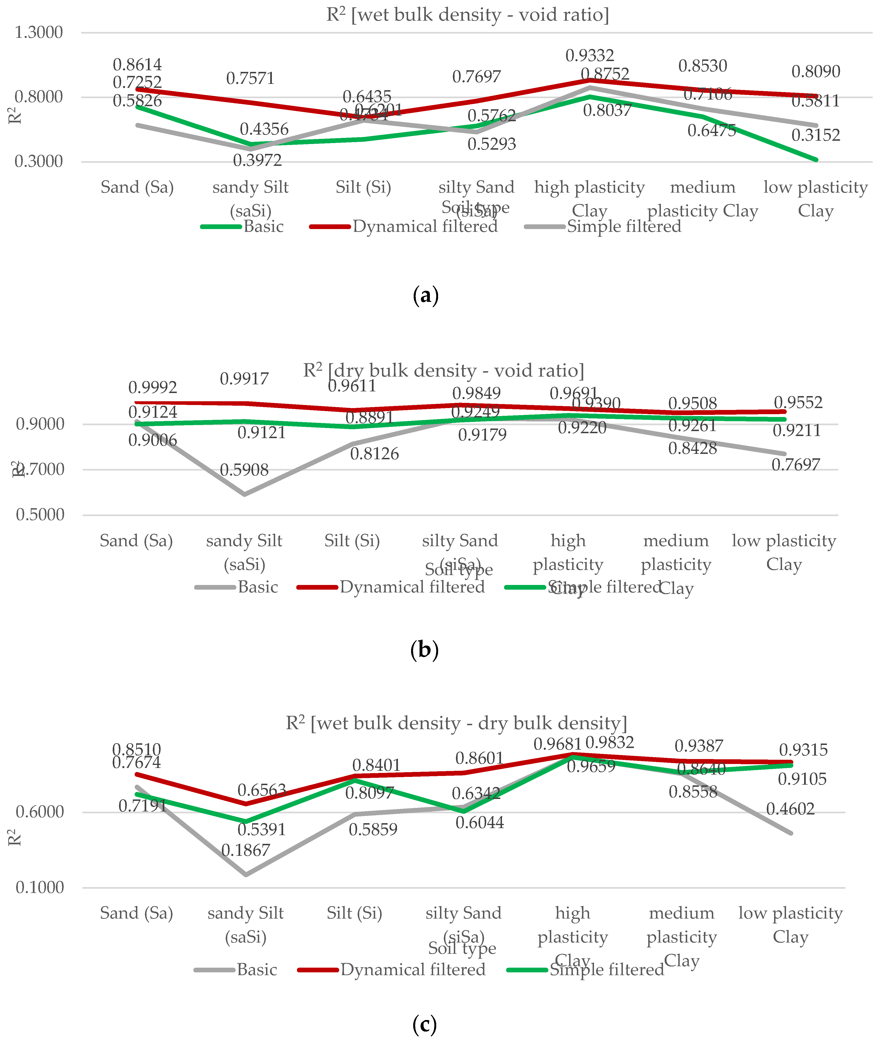
Figure 9.
Correlation Between Wet Bulk Density and Void Ratio Across Various Soil Types in the Visonta Mining Area.
Figure 9.
Correlation Between Wet Bulk Density and Void Ratio Across Various Soil Types in the Visonta Mining Area.
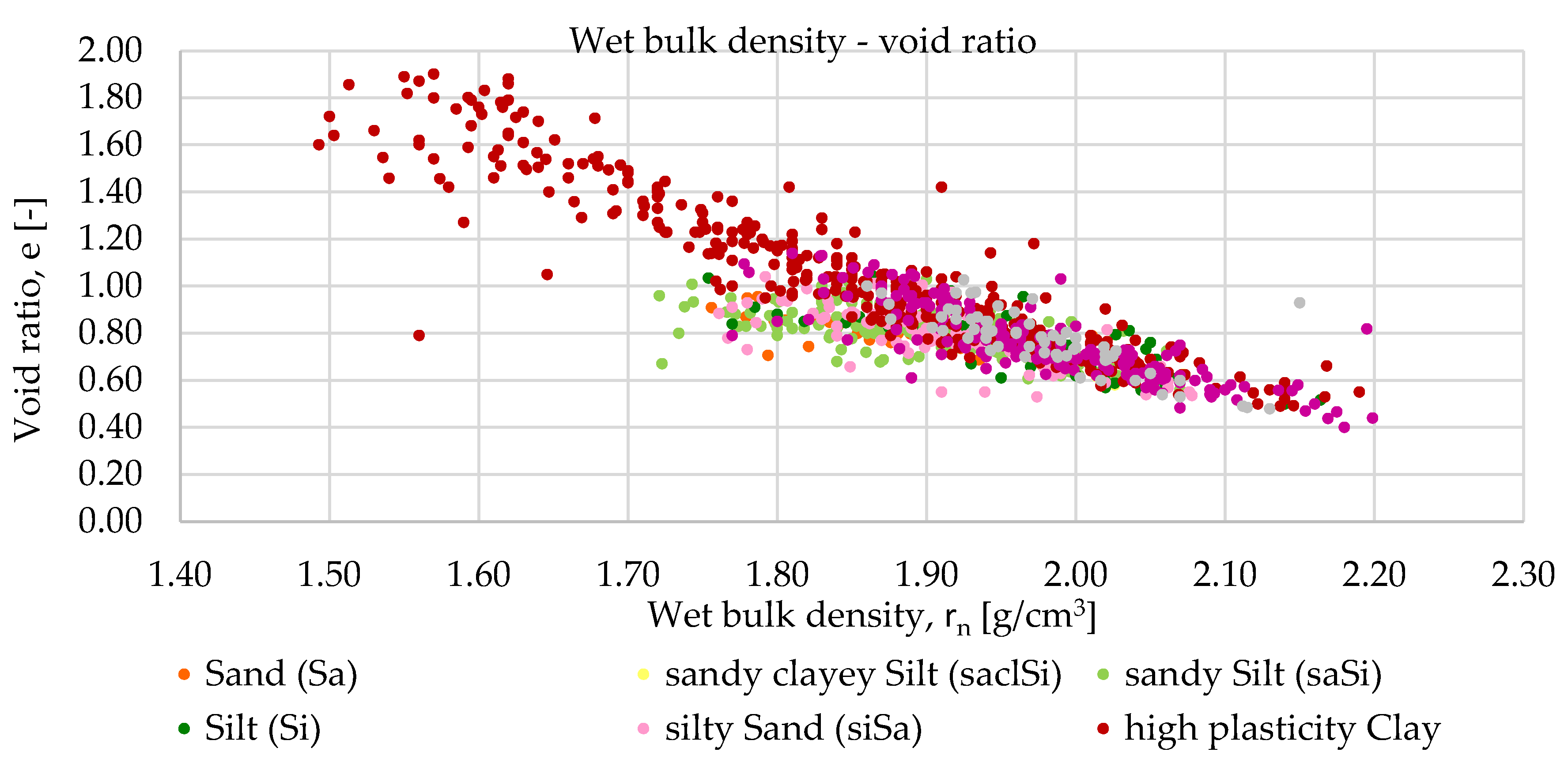
Figure 10.
Relationship Between Dry Bulk Density and Void Ratio for Various Soil Types in the Visonta Mining Area.
Figure 10.
Relationship Between Dry Bulk Density and Void Ratio for Various Soil Types in the Visonta Mining Area.
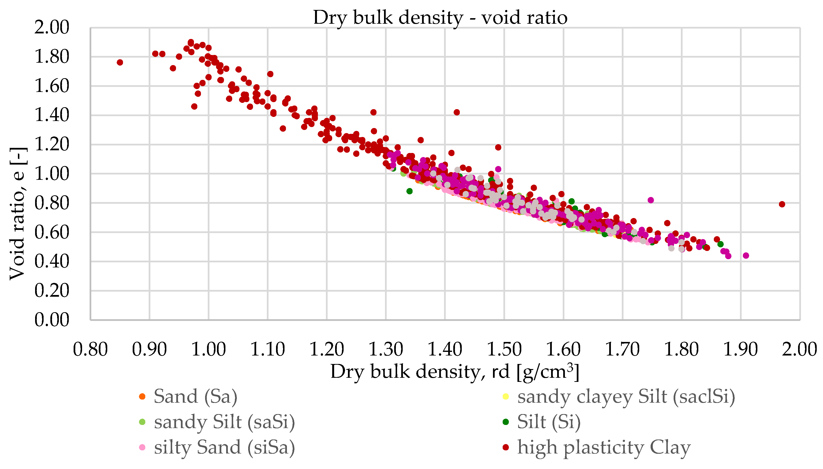
Figure 11.
Correlation Between Dry and Wet Bulk Density for Various Soil Types in the Visonta Mining Area.
Figure 11.
Correlation Between Dry and Wet Bulk Density for Various Soil Types in the Visonta Mining Area.
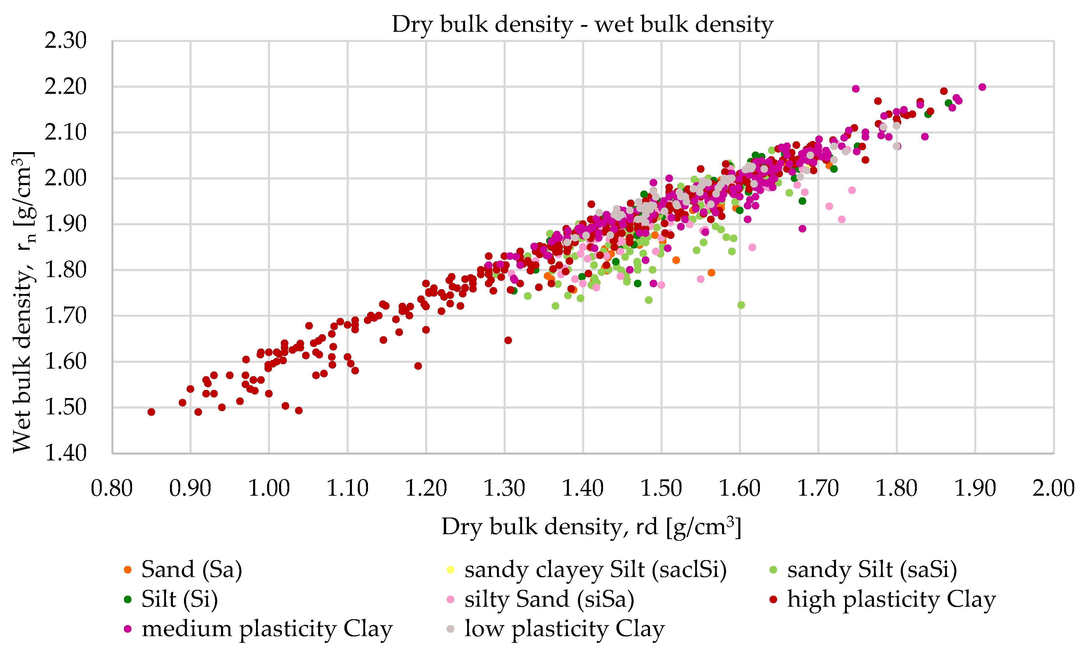
Figure 12.
Plasticity Index vs. Liquid Limit.
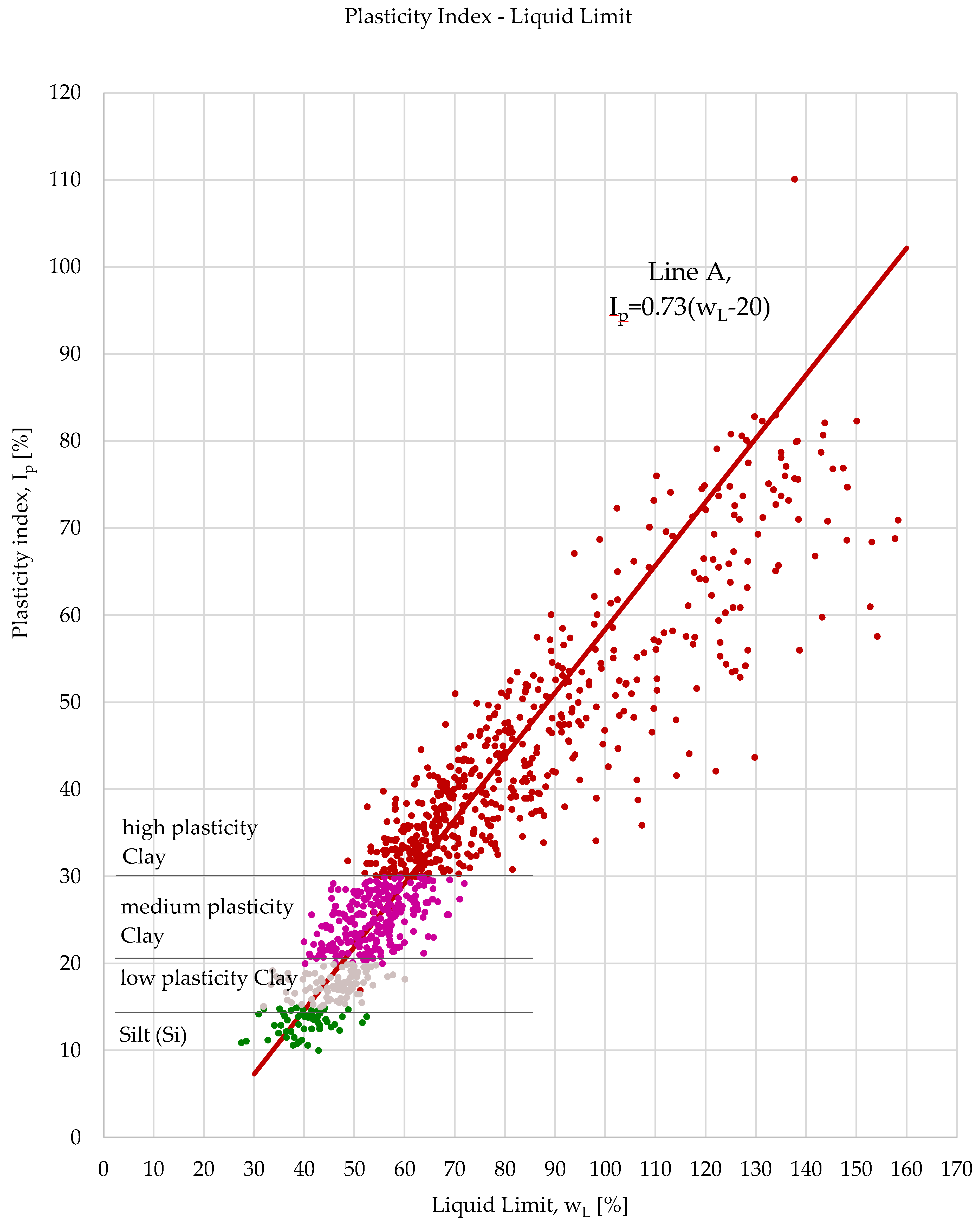
Figure 13.
Boxplot of Internal Friction Angle (f) for Different Soil Types.
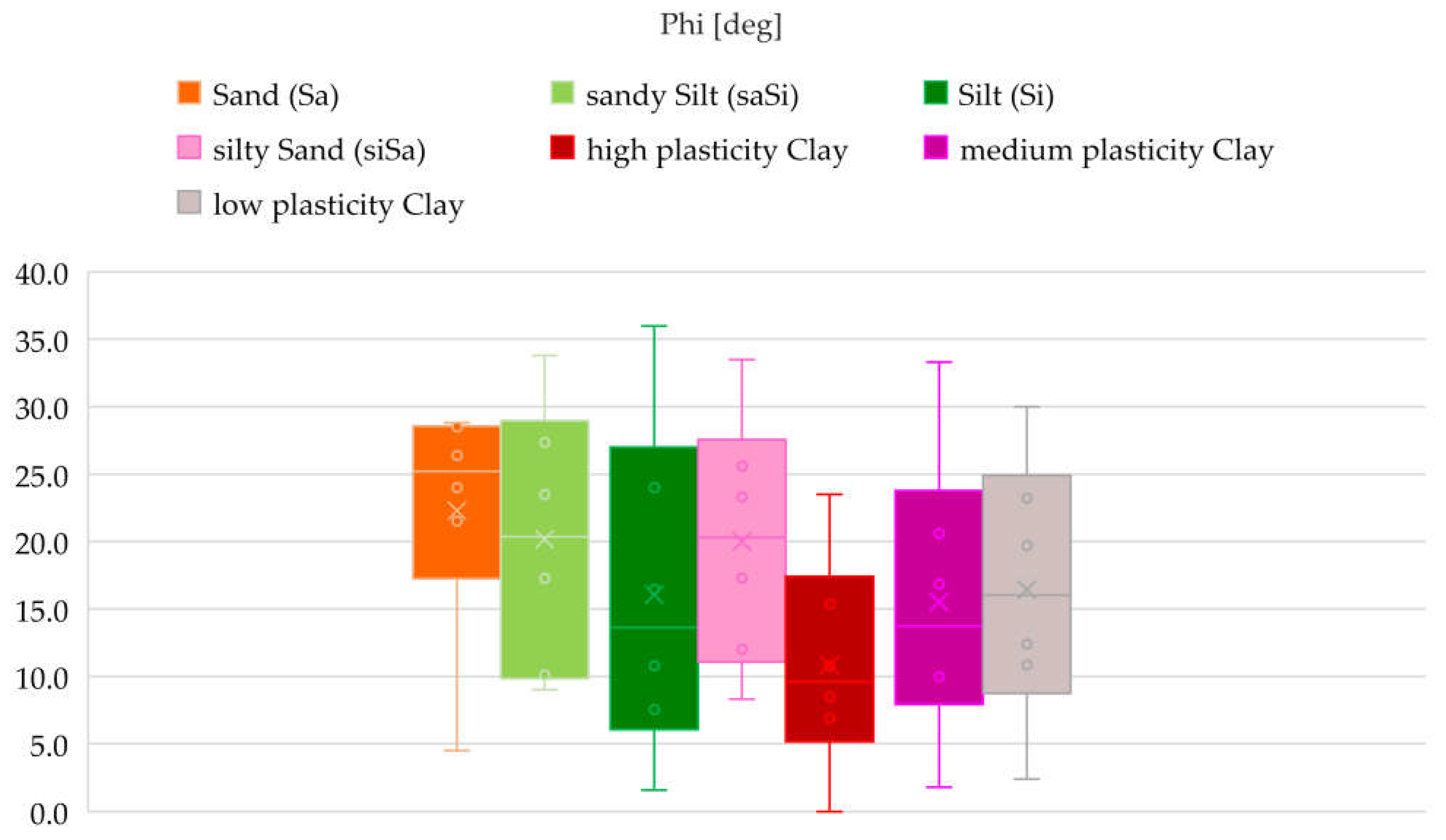
Figure 14.
Boxplot of Cohesion (kPa) for Different Soil Types.
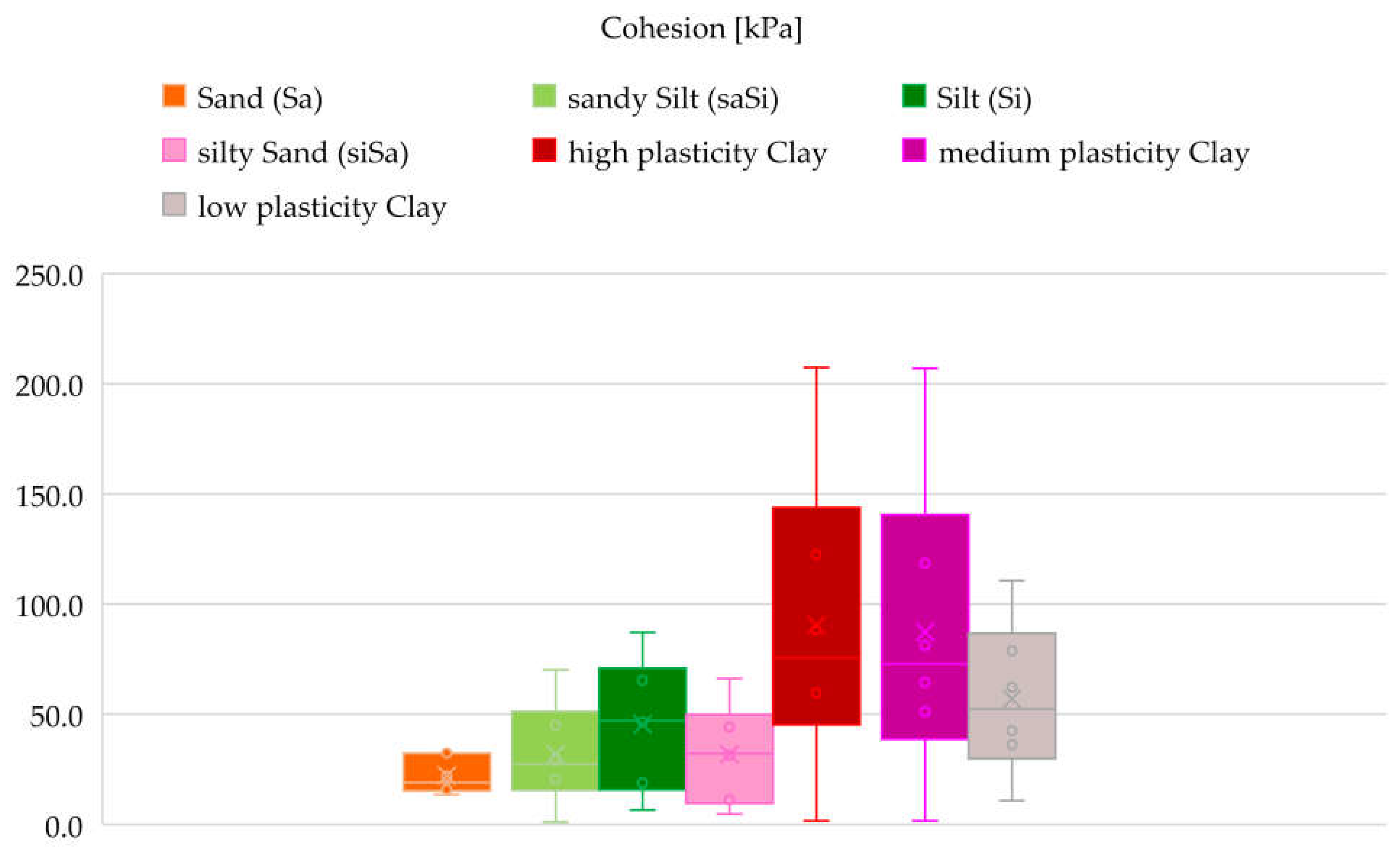
Figure 15.
Best-Fitting Probability Distributions for Unit Weight Across Soil Types Using Multiple Statistical Methods.
Figure 15.
Best-Fitting Probability Distributions for Unit Weight Across Soil Types Using Multiple Statistical Methods.
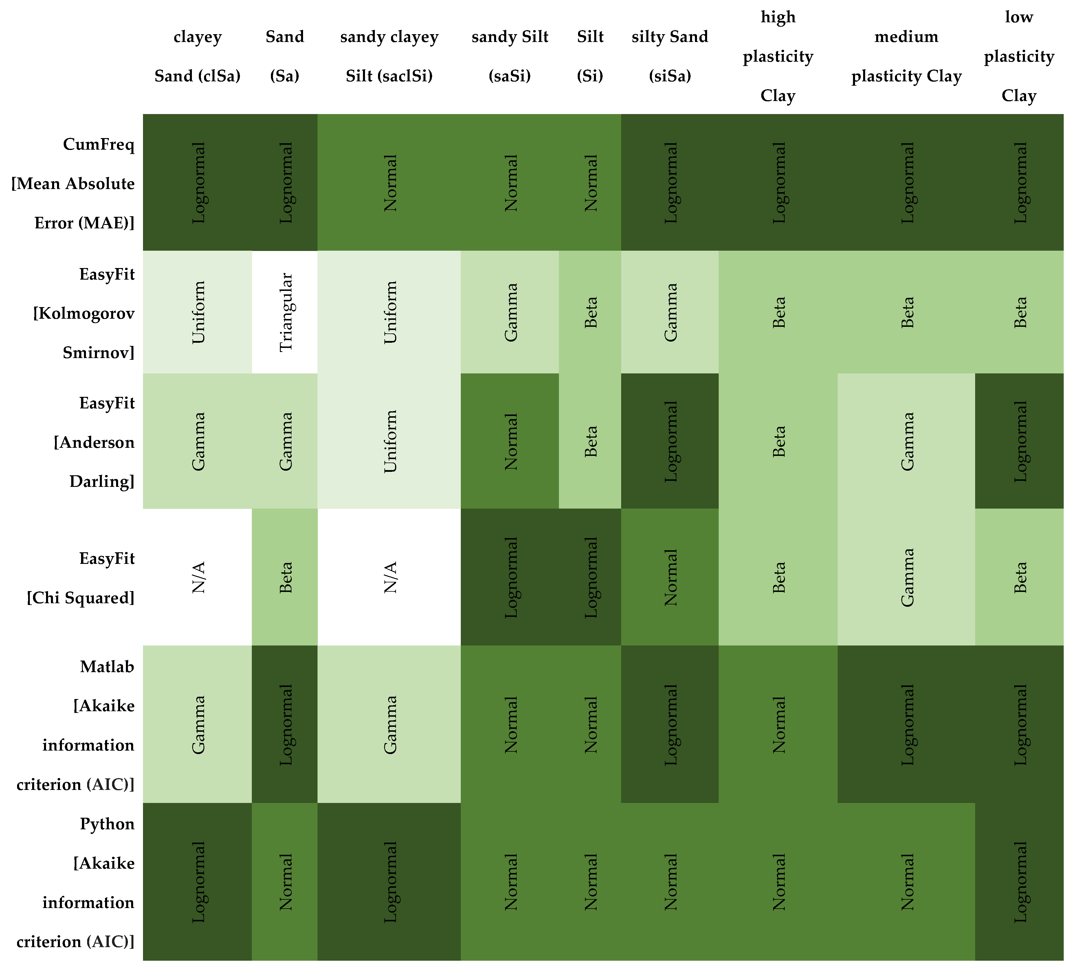
Figure 16.
Best-Fitting Probability Distributions for Shear Strength Parameters (ϕ, c) by Soil Type and Statistical Method.
Figure 16.
Best-Fitting Probability Distributions for Shear Strength Parameters (ϕ, c) by Soil Type and Statistical Method.
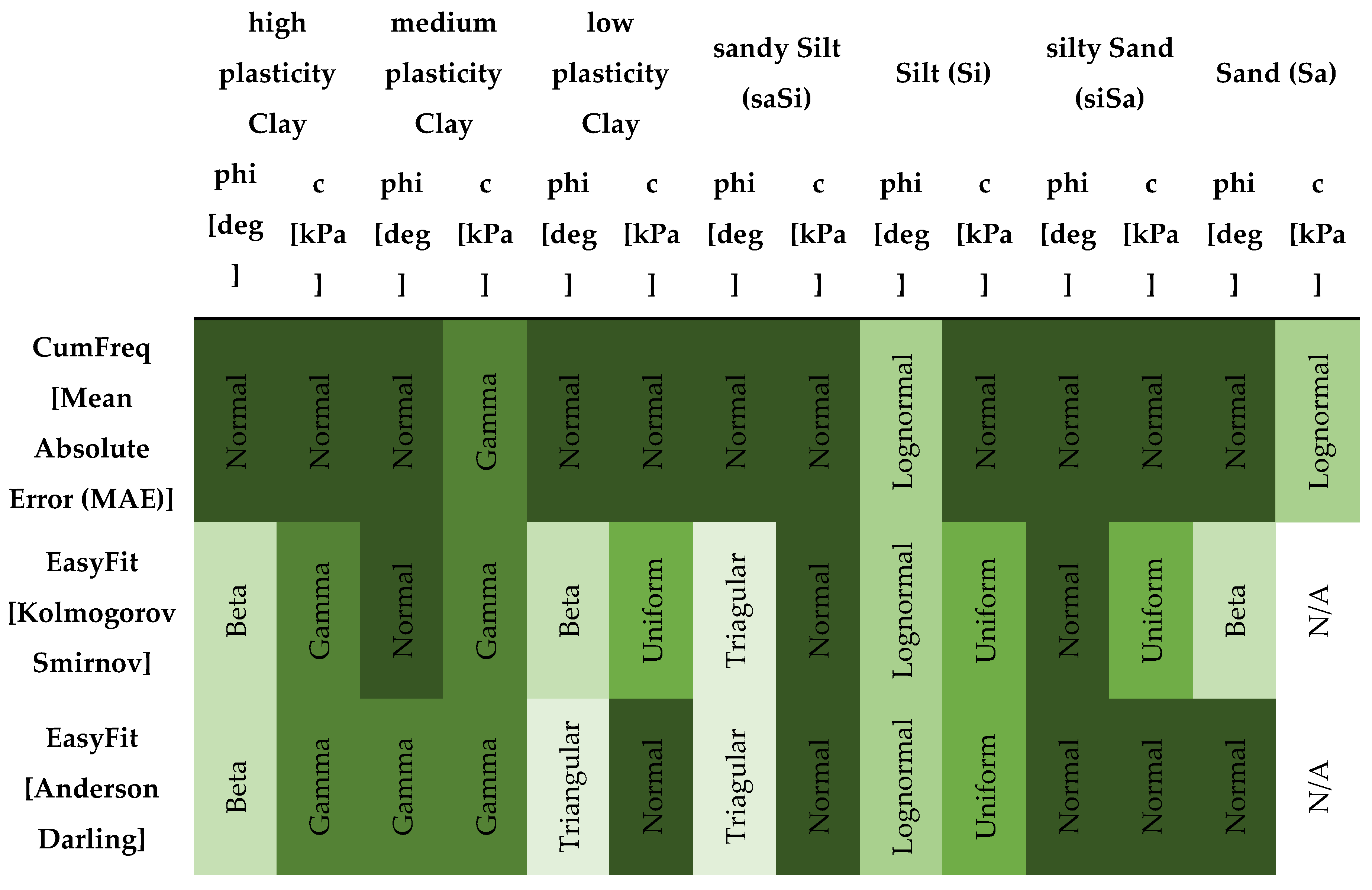
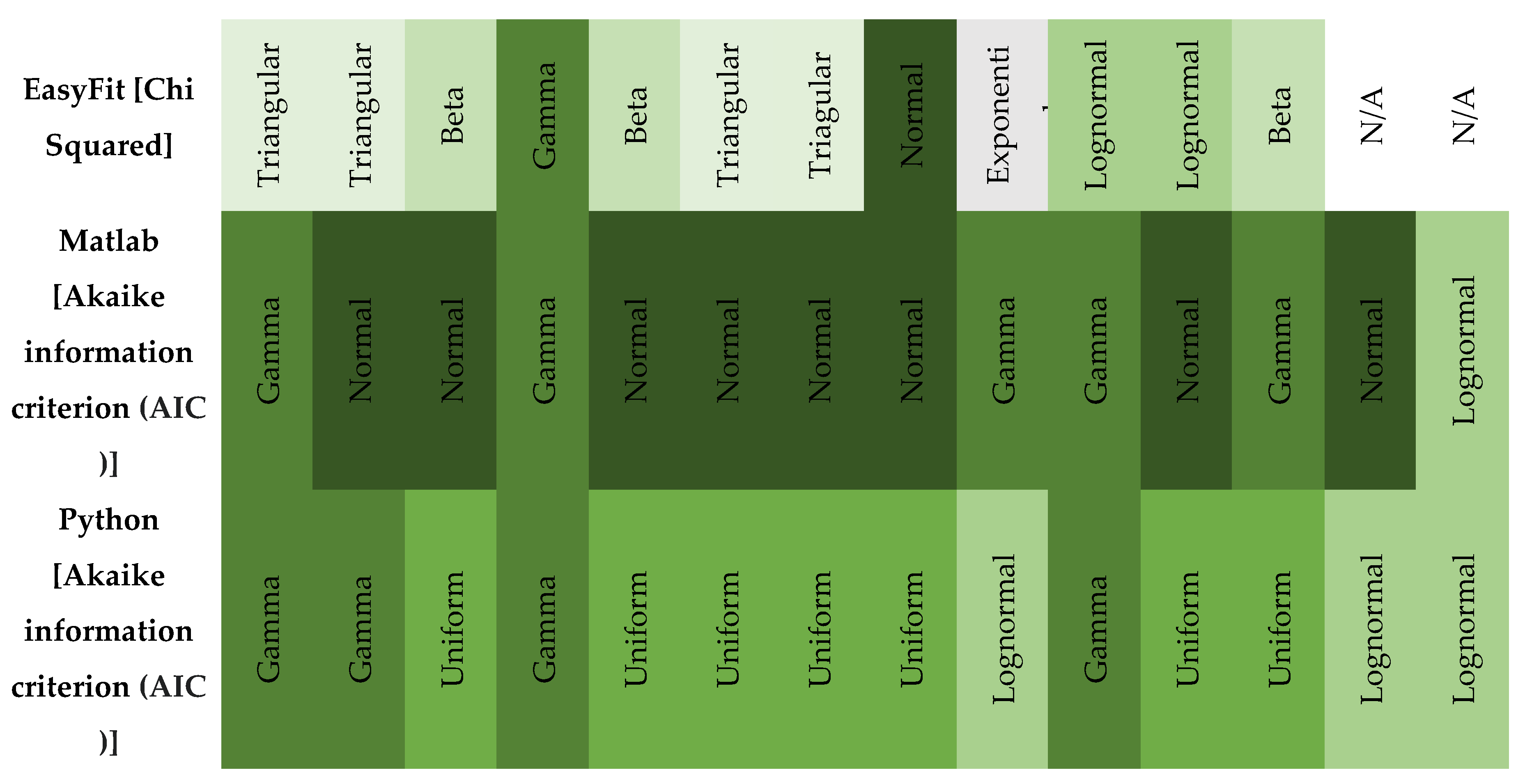
Figure 17.
Deterministic test result of Section 1.
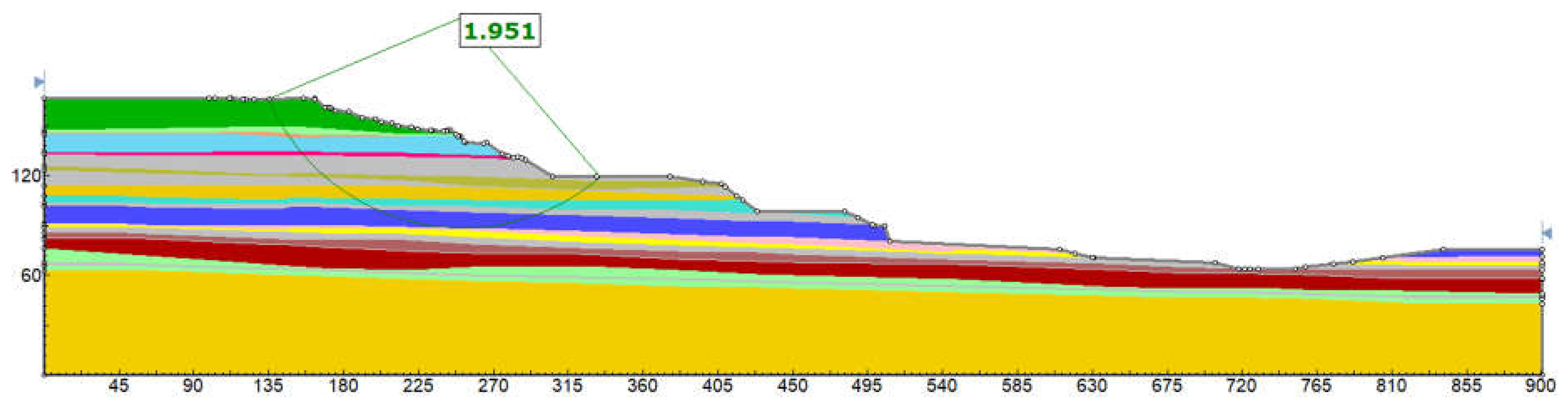
Figure 18.
Probabilistic test result of Section 1.
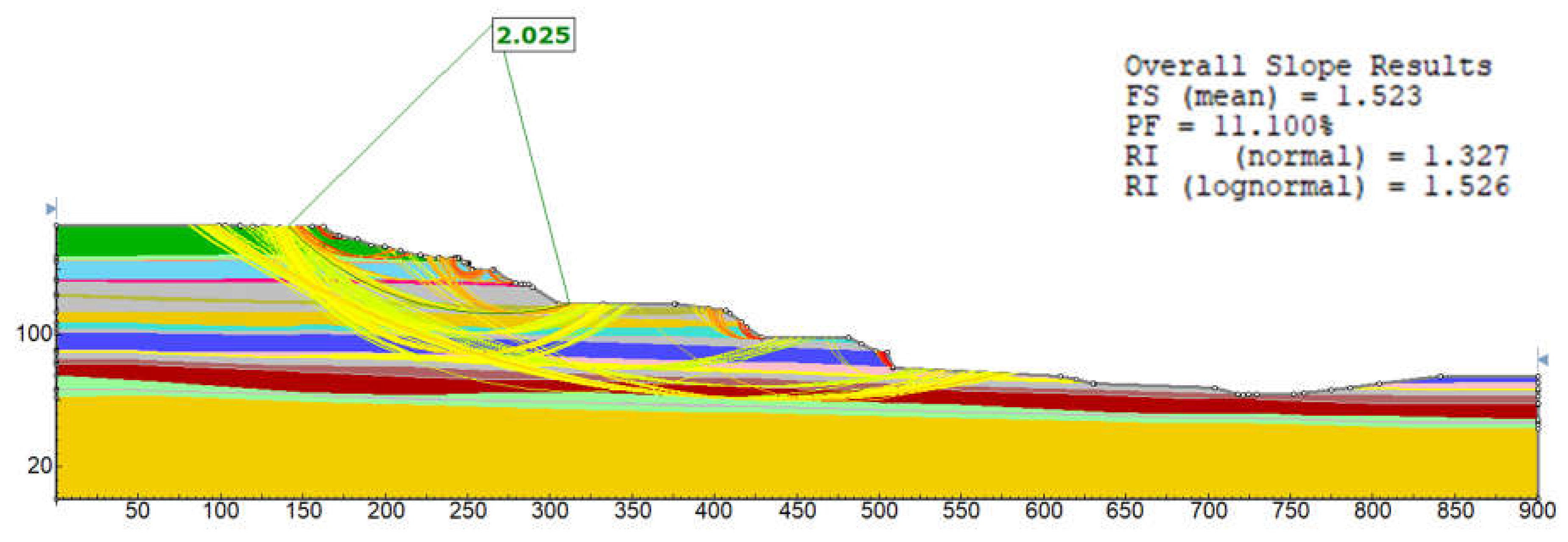
Figure 19.
Histogram of Factor of Safety (FoS) from Probabilistic Analysis Using Bishop Simplified Method (Section 1).
Figure 19.
Histogram of Factor of Safety (FoS) from Probabilistic Analysis Using Bishop Simplified Method (Section 1).
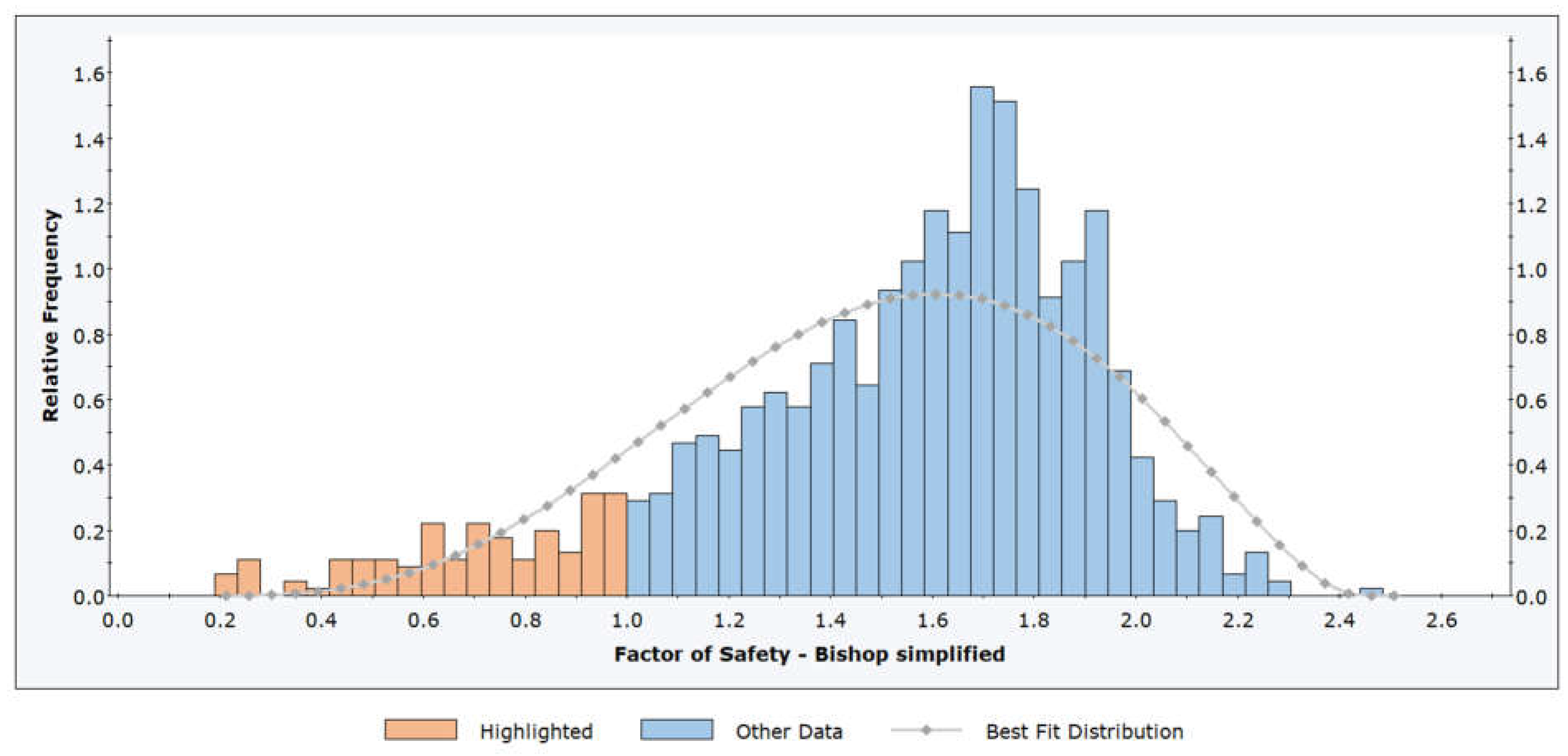
Figure 20.
Cumulative Distribution Function of Factor of Safety (FoS) from Probabilistic Analysis Using the Bishop Simplified Method (Section 1).
Figure 20.
Cumulative Distribution Function of Factor of Safety (FoS) from Probabilistic Analysis Using the Bishop Simplified Method (Section 1).
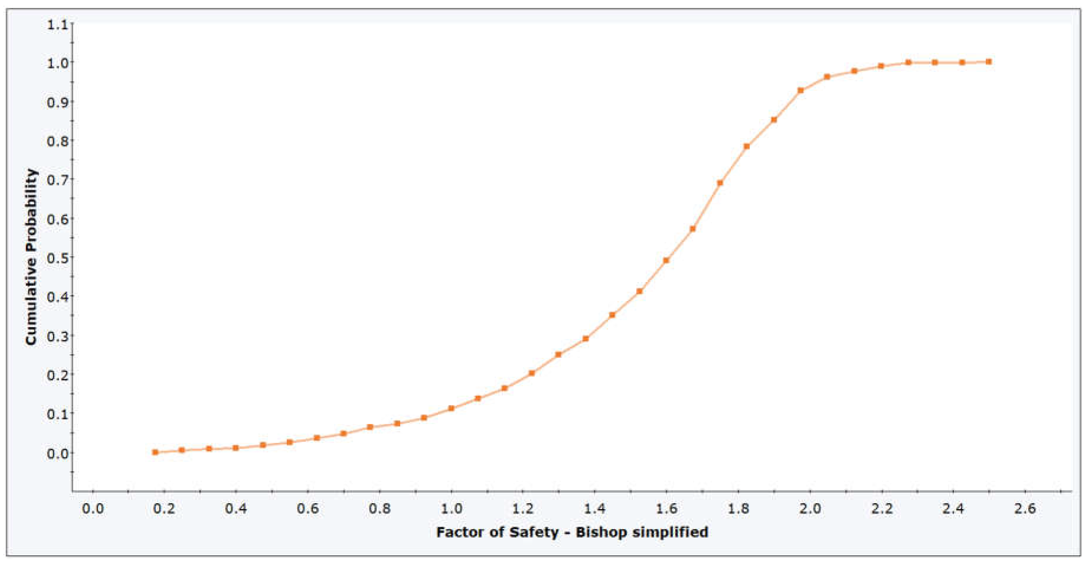
Figure 21.
Convergence of Probability of Failure with Increasing Sample Size in Latin Hypercube Simulation (Section 1).
Figure 21.
Convergence of Probability of Failure with Increasing Sample Size in Latin Hypercube Simulation (Section 1).
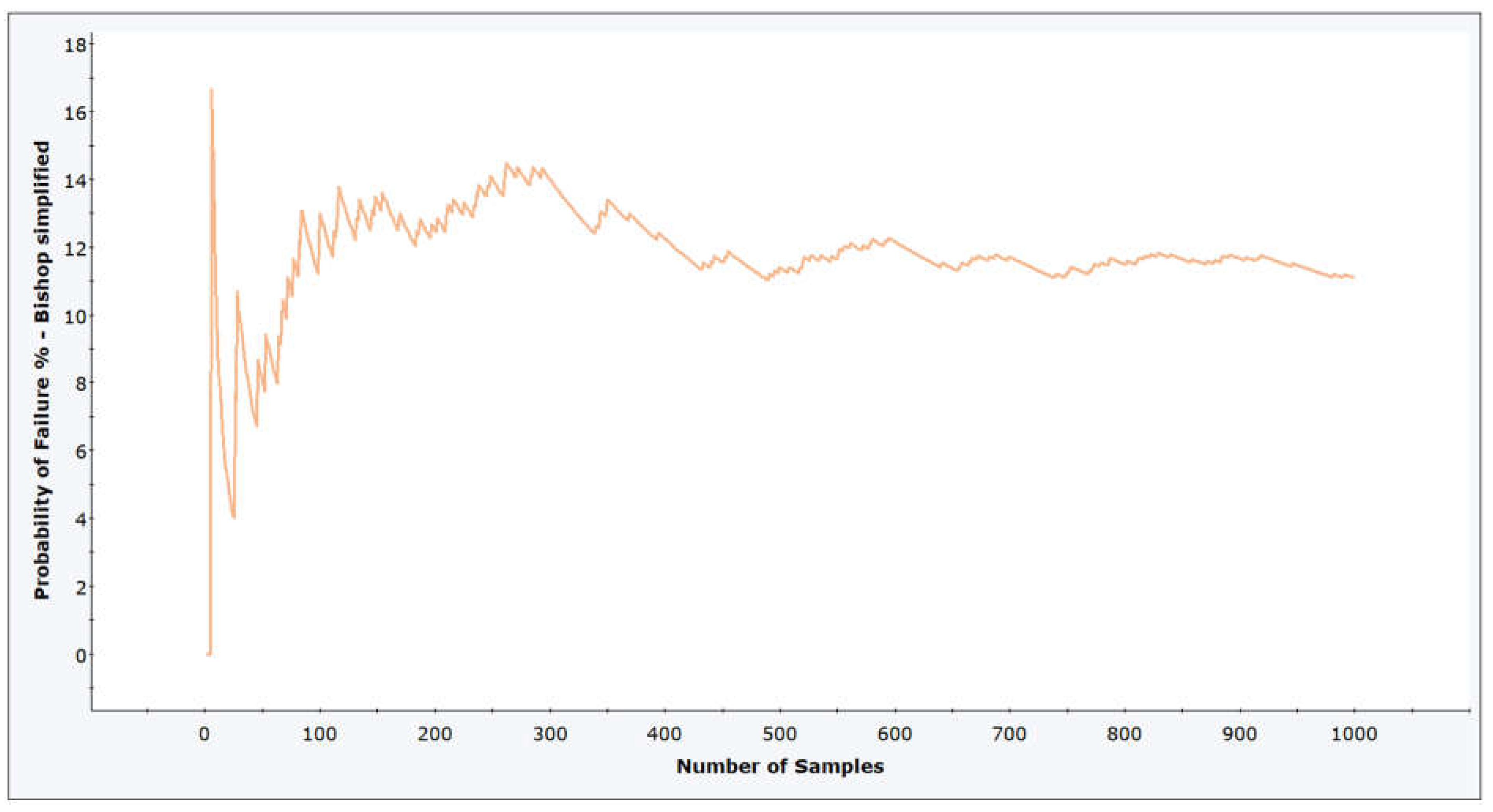
Table 1.
Number of laboratory tests on samples from the Visonta mining area.
| Borehole | 28 | |
| Drilling Depth (m) | 3305 | |
| Grain Size Distribution | 1205 | |
| Shear Testing | Internal Friction Angle f (deg) | 237 |
| Cohesion c (kPa) | 238 | |
| Residual Internal Friction frez (deg) | 264 | |
| Residual Cohesion crez (kPa) | 265 | |
| Triaxial Compression Test | Water Content W (%) | 196 |
| Saturated Bulk Density rs (g/cm3) | 155 | |
| Void Ratio e | 184 | |
| Degree of Saturation Sr | 188 | |
| Wet Bulk Density rn (g/cm3) | 205 | |
| Dry Bulk Density rd (g/cm3) | 197 | |
| Internal Friction Angle f (deg) | 166 | |
| Cohesion c (kPa) | 166 | |
| Natural Water Content - Wn (%) | 1265 | |
| Median Grain Size - Dm (mm) | 1206 | |
| Coefficient of Uniformity - Cu | 816 | |
| Grain Size Corresponding to 10% Finer - D10 (mm) | 1206 | |
| Grain Size Corresponding to 20% Finer- D20 (mm) | 1008 | |
| Grain Size Corresponding to 60% Finer (mm) | 1171 | |
| Liquid Limit - WL (%) | 653 | |
| Plastic Limit - Wp (%) | 654 | |
| Consistency Index Ic | 360 | |
| Plasticity Index - Ip (%) | 1046 | |
| Water Content - W (%) | 1225 | |
| Void Ratio - e (-) | 1258 | |
| Porosity - n (-) | 121 | |
| Degree of Saturation - Sr (-) | 1221 | |
| Dry Unit Weight - rd (g/cm3) | 1286 | |
| Wet Unit Weight - rn (g/cm3) | 1291 | |
| Undrained Shear Strength (kPa) | 471 | |
| Number of Samples | 3307 | |
Table 3.
Characteristic soil properties.
| Unit Weight (kN/m3) | Cohesion (kPa) | Phi (°) | |
|---|---|---|---|
| Quarternary Fat clay (high plasticity Clay) | 19.1 | 103 | 13 |
| Quarternary clayey Silt (clSi) | 20.0 | 56 | 22 |
| Quaternary Pannonian sandstone formation | 20.0 | 30 | 33 |
| Silt (Silt) (Si) | 20.0 | 45 | 22 |
| silty Clay (clayey Silt) (clSi) | 20.0 | 67 | 16 |
| Lignite seam | 13.0 | 100 | 26 |
| Silt (Silt) (Si) | 20.0 | 42 | 23 |
| sandy Clay (low plasticity Clay) | 19.5 | 56 | 22 |
| cover fat Clay (high plasticity Clay) | 19.5 | 103 | 13 |
| intermediate organic fat Clay (high plasticity Clay) | 20.0 | 87 | 7 |
| clayey Silt (clSi) | 20.0 | 56 | 22 |
| organic silty fat Clay (high plasticity Clay) | 20.3 | 87 | 7 |
| medium Clay (medium plasticity Clay) | 20.0 | 56 | 23 |
| bentonite fat Clay (high plasticity Clay) | 20.0 | 103 | 13 |
| sandy Silt (saSi) | 20.3 | 42 | 23 |
| aquifer (Sand) (Sa) | 20.3 | 20 | 20 |
| waste material | 17.3 | 11 | 28 |
Table 4.
Probabilitic values of Unit weight (kN/m3).
| Distribution | Mean | Std.dev. | Abs.max. | Rel.max. | Abs.min. | Rel.min. | |
|---|---|---|---|---|---|---|---|
| Quarternary Fat clay (high plasticity Clay) | Normal | 18.57 | 1.48 | 21.90 | 3.33 | 14.90 | 3.67 |
| Quarternary clayey Silt (clSi) | 20.00 | ||||||
| Quaternary Pannonian sandstone formation | 20.00 | ||||||
| Silt (Silt) (Si) | Normal | 19.56 | 0.83 | 21.64 | 2.08 | 17.54 | 2.02 |
| silty Clay (clayey Silt) (clSi) | 20.00 | ||||||
| Lignite seam | 13.00 | ||||||
| Silt (Silt) (Si) | Normal | 19.56 | 0.83 | 21.64 | 2.08 | 17.54 | 2.02 |
| sandy Clay (low plasticity Clay) | Lognormal | 19.78 | 0.62 | 21.40 | 1.62 | 18.60 | 1.18 |
| cover fat Clay (high plasticity Clay) | Normal | 18.57 | 1.48 | 21.90 | 3.33 | 14.90 | 3.67 |
| intermediate organic fat Clay (high plasticity Clay) | Normal | 18.57 | 1.48 | 21.90 | 3.33 | 14.90 | 3.67 |
| clayey Silt (clSi) | 20.00 | ||||||
| organic silty fat Clay (high plasticity Clay) | Normal | 18.57 | 1.48 | 21.90 | 3.33 | 14.90 | 3.67 |
| medium Clay (medium plasticity Clay) | Lognormal | 19.70 | 0.88 | 21.99 | 2.29 | 17.36 | 2.34 |
| bentonite fat Clay (high plasticity Clay) | Normal | 18.57 | 1.48 | 21.90 | 3.33 | 14.90 | 3.67 |
| sandy Silt (saSi) | Normal | 19.04 | 0.70 | 20.70 | 1.66 | 17.34 | 1.70 |
| aquifer (Sand) (Sa) | Lognormal | 18.99 | 0.68 | 20.33 | 1.34 | 17.56 | 1.43 |
| waste material | 17.30 |
Table 5.
Probabilistic Cohesion (kPa) values.
| Distribution | Mean | Std.dev. | Abs.max. | Rel.max. | Abs.min. | Rel.min. | |
|---|---|---|---|---|---|---|---|
| Quarternary fat clay (high plasticity Clay) | Normal | 91.4 | 43.1 | 207.4 | 116 | 1.7 | 89.7 |
| Quarternary clayey Silt (clSi) | 56.0 | ||||||
| Quaternary Pannonian sandstone formation | 30.0 | ||||||
| Silt (Silt) (Si) | Gamma | 46.1 | 31 | 87.1 | 41 | 6.6 | 39.5 |
| silty Clay (clayey Silt) (clSi) | 67.0 | ||||||
| Lignite seam | 100.0 | ||||||
| Silt (Silt) (Si) | Gamma | 46.1 | 31 | 87.1 | 41 | 6.6 | 39.5 |
| sandy Clay (low plasticity Clay) | Normal | 58.3 | 28.7 | 110.6 | 52.3 | 10.9 | 47.4 |
| cover fat Clay (high plasticity Clay) | Normal | 91.4 | 43.1 | 207.4 | 116 | 1.7 | 89.7 |
| intermediate organic fat Clay (high plasticity Clay) | Normal | 91.4 | 43.1 | 207.4 | 116 | 1.7 | 89.7 |
| clayey Silt (clSi) | 56.0 | ||||||
| organic silty fat Clay (high plasticity Clay) | Normal | 91.4 | 43.1 | 207.4 | 116 | 1.7 | 89.7 |
| medium Clay (medium plasticity Clay) | Gamma | 86.3 | 49.9 | 207 | 120.7 | 1.7 | 84.6 |
| bentonite fat Clay (high plasticity Clay) | Normal | 91.4 | 43.1 | 207.4 | 116 | 1.7 | 89.7 |
| sandy Silt (saSi) | Normal | 30.9 | 17.2 | 70 | 39.1 | 1.3 | 29.6 |
| aquifer (Sand) (Sa) | Lognormal | 21.3 | 8.4 | 32.3 | 11 | 13.5 | 7.8 |
| waste material | 11.0 |
Table 6.
Probabilistic values of internal friction angle Phi (deg) values.
| Distribution | Mean | Std.dev. | Abs.max. | Rel.max. | Abs.min. | Rel.min. | |
|---|---|---|---|---|---|---|---|
| Quarternary fat clay (high plasticity Clay) | Gamma | 11.00 | 5.80 | 23.50 | 12.50 | 0.00 | 11.00 |
| Quarternary clayey Silt (clSi) | 22.00 | ||||||
| Quaternary Pannonian sandstone formation | 33.00 | ||||||
| Silt (Silt) (Si) | Lognormal | 15.20 | 10.40 | 36.00 | 20.80 | 1.60 | 13.60 |
| silty Clay (clayey Silt) (clSi) | 16.00 | ||||||
| Lignite seam | 26.00 | ||||||
| Silt (Silt) (Si) | Lognormal | 15.20 | 10.40 | 36.00 | 20.80 | 1.60 | 13.60 |
| sandy Clay (low plasticity Clay) | Lognormal | 22.71 | 1.72 | 25.80 | 3.09 | 21.10 | 1.61 |
| cover fat Clay (high plasticity Clay) | Gamma | 11.00 | 5.80 | 23.50 | 12.50 | 0.00 | 11.00 |
| intermediate organic fat Clay (high plasticity Clay) | Gamma | 11.00 | 5.80 | 23.50 | 12.50 | 0.00 | 11.00 |
| clayey Silt (clSi) | 22.00 | ||||||
| organic silty fat Clay (high plasticity Clay) | Gamma | 11.00 | 5.80 | 23.50 | 12.50 | 0.00 | 11.00 |
| medium Clay (medium plasticity Clay) | Normal | 17.70 | 6.69 | 33.30 | 15.60 | 4.00 | 13.70 |
| bentonite fat Clay (high plasticity Clay) | Gamma | 11.00 | 5.80 | 23.50 | 12.50 | 0.00 | 11.00 |
| sandy Silt (saSi) | Normal | 26.22 | 3.52 | 30.00 | 3.78 | 20.00 | 6.22 |
| aquifer (Sand) (Sa) | Normal | 25.80 | 3.10 | 28.80 | 3.00 | 21.50 | 4.30 |
| waste material | 28.00 |
Table 8.
Probabilistic test results of all Sections.
| Section 1 | Section 2 | Section 3 | Section 4 | Section 5 | Section 6 | Section 7 | |
|---|---|---|---|---|---|---|---|
| FS [-] | 2.025 | 1.207 | 2.060 | 1.647 | 1.729 | 1.583 | 1.334 |
| FS (mean) | 1.523 | 1.019 | 1.542 | 1.216 | 1.243 | 1.579 | 1.334 |
| PF [%] | 11.1% | 46.7% | 9.0% | 28.6% | 23.3% | 0.0% | 0.0% |
| RI (normal) | 1.327 | 0.063 | 1.411 | 0.61 | 0.745 | 41.571 | - |
| RI (lognormal) | 1.526 | -0.079 | 1.643 | 0.542 | 0.714 | 51.781 | - |
Disclaimer/Publisher’s Note: The statements, opinions and data contained in all publications are solely those of the individual author(s) and contributor(s) and not of MDPI and/or the editor(s). MDPI and/or the editor(s) disclaim responsibility for any injury to people or property resulting from any ideas, methods, instructions or products referred to in the content. |
© 2025 by the authors. Licensee MDPI, Basel, Switzerland. This article is an open access article distributed under the terms and conditions of the Creative Commons Attribution (CC BY) license (http://creativecommons.org/licenses/by/4.0/).
Copyright: This open access article is published under a Creative Commons CC BY 4.0 license, which permit the free download, distribution, and reuse, provided that the author and preprint are cited in any reuse.


