
Submitted:
04 May 2025
Posted:
07 May 2025
You are already at the latest version
Abstract
Longstanding anomalies in the Cosmic Microwave Background (CMB), including the low quadrupole moment and hemispherical power asymmetry, have recently been linked to an underlying parity asymmetry. We show here how this parity asymmetry naturally arises within a quantum framework that explicitly incorporates PT symmetry—parity (P) and time-reversal (T). This additional symmetry restores unitarity in quantum field theory (QFT) in curved spacetime. When applied to inflationary quantum fluctuations, this extended symmetry predicts parity asymmetry as a natural consequence of cosmic expansion, which inherently breaks time-reversal symmetry. Observational data strongly favor this unitary approach, with a likelihood ratio exceeding 650 times that of predictions from the standard inflationary framework. These results provide compelling evidence for the quantum gravitational origins of CMB parity asymmetry.
Keywords:
Cosmology
; CMB
; QFT
; General Relativity
; Inflation
1. Introduction
Understanding and testing the interplay between gravity and quantum mechanics (QM) is the most important key to unraveling the new physics beyond the standard model of particle physics and Einstein’s general relativity (GR). The merge of GR and QM is an essential physics that can be unlocked at the length scales of gravitational horizons. For this, we perhaps need an in-depth understanding of how one can resolve an age-old conundrum in the concept of time between the GR and QM. The success of Quantum field theory (QFT) in Minkowski spacetime ([1]) already teaches us several lessons in this regard. Indeed, QFT is the culmination of special relativity (SR) and QM, where the concept of time already enters into the conflict. In SR, the space and time are on equal footing, but in QM, spatial coordinates are elevated to operators while time is just a parameter due to its anti-unitary nature under the discrete transformation (). The SR and QM are merged by imposing the commutativity of operators corresponding to space-like distances. The underlying reason is that SR forbids any communication happening in space-like distances, and we respect it and achieve it by formulating new mathematical rules via second quantization. This is exactly the lesson one must keep in mind to understand quantum fields in curved spacetime. That is, we take lessons from classical physics and comply with them according to the rules of quantum physics. The quantum field theory in curved spacetime (QFTCS) is the first step in seeing GR and QM acting together besides the renormalizable ultra-violet complete quantum gravity that may be required at the Planck scales. Furthermore, QFTCS is a necessity in the context of understanding inflationary quantum fluctuations ([2,3,4]).
In this paper, we address crucial questions related to the meaning of time reversal and parity inversions in the context of inflationary background spacetime to place quantum fields on it and uncover their true nature in the cosmic microwave background (CMB). We explain how direct-sum quantum field theory (DQFT), [5,6,7]) is a necessity to solve the unitarity problem of QFTCS. The question of unitarity in QFTCS precedes the question of a completely renormalizable quantum gravity theory of Planck scales. In contrast to the widespread schools of thought that argue unitarity in QFTCS needs to be given up within GR and QM, we propose a new fundamental understanding of this issue and a new observational test using the parity asymmetry in the CMB. We find that the theory of inflationary quantum fluctuations with DQFT (which we call shortly DSI, which stands for "Direct-Sum inflation") fits up to 650 times better than the Standard Inflation (SI). This paper ultimately presents the picture of how a new theory of QFTCS emerged from fundamental questions of quantum gravitational physics that can potentially explain the observed CMB large-scale anomalies. The new results in this paper are further complemented by our more extended companion paper ([8]).
2. DQFT, in a Nutshell ()
DQFT formulation emerges from a simple reconstruction of a quantum state or a quantum field operator through the discrete (a)symmetries (parity and time reversal ) of the background spacetime. Here, we summarize the conceptual understanding of DQFT and direct the reader to [5,6,7,8] for more details. Construction of QFT in Minkowski spacetime requires the definition of positive energy state and the arrow of time [9]. Here, we build quantum theory with two arrows of time using the direct-sum Schrödinger equation
where is the time-independent Hamiltonian operator (which is Hermitian) that is symmetric. The quantum state is the direct-sum of two components
where are the two components of the same state at parity conjugate points. The component is a positive energy state that evolves forward in time as where the parametric time arrow while can also be seen as a positive energy state that evolves back in time as with the parametric time convention . One can notice here the purely antiunitary character of time associated with the replacement ([9]). The direct-sum Schrödinger equation does not have any arrow of time associated with it compared to the conventional Schrödinger equation. The direct-sum splitting of the quantum state as in Eq.2 implies the Hilbert space () splitting into a direct-sum of the two () corresponding to parity conjugate points in position space: . Here, the Hilbert spaces are called the geometric superselection sectors ([5,7]). The position and momentum commutation relations now become double associated with parity conjugate position and momentum space operators denoted by subscripts , and their relations are
This framework only makes the wavefunction of the quantum system explicitly symmetric that resonates with the assumed symmetry of the physical system, i.e. and the results of standard quantum mechanics remain the same as shown with the example of harmonic oscillator worked out in [8] (see also further discussions and Fig.1 in [5]). The DQFT in Minkowski spacetime ( which is symmetric) is just built on the direct-sum Schrödinger equation, following how the standard QFT is built on the definition of positive energy state and the causality condition (i.e., commutativity of operators for spacelike distances). See Appendix A for more details.
3. DQFT in de Sitter & Unitarity ()
The de Sitter (dS) spacetime is a perfect testing ground for exploring the theory of QFTCS because of its maximally symmetric aspect, and it is also relevant for unlocking the nature of inflationary quantum fluctuations. Furthermore, a dS spacetime has the closest resemblance with black holes, where the most important conundrums in quantum physics emerge such as the loss of unitarity and the information-loss paradox. We start with the dS metric in the flat Friedman-Lemaître-Robertson-Walker (FLRW) coordinates
where the scale factor is the clock that determines the expansion of the Universe, is the Hubble parameter and is the conformal time. If one has to place quantum theory in dS spacetime Eq.4 the first and foremost things to be understood are the parity and time reversal operations. The usual conception of understanding the expansion of the Universe is to restrict ourselves to . But the metric carries a symmetry
Restricting to before quantization of a classical field (as is usually followed in standard QFTCS) means throwing away the symmetry in Eq.5 by hand. The expanding Universe can be realized in two ways:
This would explain why in the Wheeler-de Witt equation the cosmic time does not explicitly appear, rather the scale factor is the clock that runs with expanding Universe ([10]). Note that does not change any properties of the dS space at all. For example, curvature invariants such as the Ricci scalar remain the same under a discrete sign flip of H. Eq.6 illustrates two possible time realizations for an expanding universe. By convention, choosing or results in loss of information beyond the horizon. In his famous monograph of 1956, Schrodinger [11] rejected the idea of two universes because it would lead to a conundrum of ignorance of information beyond the horizon, which in modern language means pure states evolving into mixed states which leads the violation of unitarity and information-loss ([12,13]).
Similar to the Minkowski space (see Appendix A), the quantum fields in the dS space are described through a direct-sum vacuum corresponding to the direct-sum Fock space . This implies that everywhere in dS space, a quantum field is tied by time forward and backward evolutions at the parity conjugate points, see Appendix B. At any moment of dS expansion, the parity-conjugate points on the comoving horizon are space-like separated for an imaginary classical observer as shown in Figure 1.
Note that by DQFT construction, the direct-sum quantum states that follow from Eq.A6 are the opposite time evolving positive energy states at the parity conjugate points and this holds for any imaginary classical observer. Furthermore, in DQFT the causality and locality are preserved too. A consequence of this is that any state that disappears beyond the horizon happens to be the complimentary direct-sum (component) state that reappears at the antipodal point. This is because all the imaginary classical observers, including those on the horizons of each other, should observe the same direct-sum quantum state .
This means the horizon acts as a mirror which maps every information outside the horizon to the states inside the horizon. To see this, consider a pure state:
where are the eigenvectors, i.e. for any observable (an operator) we have: where are the corresponding eigenvalues. Each will be observed in with a probability: . Consider now the (deSitter) Hubble horizon around an observer (as illustrated in Figure 1). In the standard approach, information is lost (a pure state becomes a mix state) because communication can not happen for space-like distances (i.e. outside the horizon) as was shown by Gibbons and Hawking in 1977 [12], in analogy to what happens in Hawking radiation and the black hole information loss paradox [6,14]. This also implies the lost of unitarity in QFT on spacetimes with horizons. In the DQFT approach we have:
where are the eigenvectors corresponding to each separated Hilbert space. So that the observable probabilities and operators become:
Information is not lost in this case because there is not entanglement across the horizon. To see this more clearly, consider the case where is a pure entangled system :
where ⊗ represents the tensor product of two Hilbert spaces A and B which are entangled (inseparable or correlated): with: and . For example, a pair of particles (across the horizon). In the DQFT approach, we have:
where and are the eigenvectors corresponding to each separated Hilbert spaces, which remain within the horizon because no information is exchanged across separated spaces. All information about the entanglement pairs is mapped within the horizon; thus, the pure state will remain pure. In other words, DQFT forbids any entanglement beyond the gravitational horizons. DQFT constructs a direct-sum Hilbert space with the interior and exterior separated by a geometric superselection rule (which is similar to the concept of superselection sectors in QFT [15,16]). Thus, there would be an observer complementarity (see Fig.3 in [5]). We can also understand the same from the point of view of dS space in static coordinates, which reads as
where and . The relation between the flat FLRW Eq.4 and Eq.12 is just a simple coordinate change ([17,18]). A very practiced view of flat dS spacetime in Eq.4 is that it covers only half of the dS space. However, we must keep in mind the symmetry in Eq.6, which implies that Eq.4 can cover the entire dS space. Thus, the maximally symmetric nature of the dS spacetime sets no difference whether it is expressed in flat, closed, open FLRW coordinates or the static coordinates ([19]). The use of mapping flat coordinates to static coordinates here is so that we can realize how unitarity can be achieved with DQFT, whereas it is lost in standard QFT, as was shown by Gibbons and Hawking in 1977 [12]. In Figure 2, we show unitary quantum physics in the static dS space through the (quantum) conformal diagram, where we see the three-dimensional space divided by parity for the interior and exterior of the cosmological event horizon. We can picture here how none of the observers loses any information beyond the horizon. If any state leaves the horizon, it is only the (complimentary) direct-sum component of what is inside the horizon. This means that any observer can perfectly reconstruct the information about what is beyond the horizon. According to DQFT, every density matrix of a maximally entangled pure state is split into direct-sum of 4 components
Each density matrix is defined by a pure state component in the corresponding (geometric) superselection sector Hilbert space . Since Von Neumann entropy of each component of density matrix vanishes , any observer in regions I, II, III, IV (see Figure 2) would witness pure states evolving into pure states. Thus, with DQFT we can have both unitarity and observer complementarity in dS ([5]).
According to DQFT, any state is spread across the horizon by distinct components in geometric superselection sectors. This implies that any information of the entangled state is shared by the sectorial Hilbert space, leading to pure states evolving into pure states. To be precise, the Hilbert spaces of the interior and exterior states cannot be connected by direct product (⊗) but rather should be related by direct-sum (⊕). This has to be like this because beyond-the-horizon time is not the same, so one cannot do the same quantum mechanics everywhere. In other words, the gravitational horizons are special, they separate different spacetimes by a boundary. Thus, they cannot be treated as a standard null surface, where quantum states can be entangled across. Furthermore, we stress that no entanglement across the horizon does not lead to firewalls, which happens in standard QFTCS but not in direct-sum QFTCS. For further analogous discussion on unitarity and no information loss in the context of the Schwarzschild black hole, see [6]. In a nutshell, DQFT offers a new understanding of dS space where any observer’s physics of the universe is complete, and no information is lost outside any observer’s universe. This is exactly what Schrödinger envisioned in 1956 for a quantum theory to achieve [11]. Furthermore, our achievement of DQFT echoes well with the recent classical understanding of dS through the Black Hole Universe (BHU) proposal [20,21,22].
4. CMB Parity Asymmetry
Inflationary quantum fluctuations are the initial seeds for large-scale structure formation. It is important to understand their quantum nature to derive consistent CMB predictions. Inflation is by definition a quasi-dS expansion ([23]) and this means that in Eq.6 is spontaneously broken by the presence of a non-perturbative scalar field in addition to the GR’s tensor degree of freedom. Our focus here is on single-field inflation. The metric and scalar field matter quantum fluctuations are generated during inflation. The quantity which is a gauge-invariant combination of them is called the curvature perturbation (), and it is an effective (scalar) degree of freedom. It connects the quantum physics of inflation to CMB observations. The action for curvature perturbation at the linear order is
where which is nearly constant during inflation characterized by the smallness of slow-roll parameters for number of e-foldings. The canonical variable which is a redefinition of curvature perturbation that we eventually quantize is
In the framework of Direct-sum Inflation (DSI), the canonical variable is promoted to field operator that is split into direct-sum of two components
which generate quantum fields in a direct-sum vacuum
in which they evolve forward and backward in time at the parity conjugate points in physical space. In analogy with Eq.6, the time reversal operation (quantum mechanically) in an expanding quasi-dS Universe is
These sign differences in the slow-roll parameters, which break the time-reversal symmetry of de Sitter spacetime, lead to corrections in the evolution of quantum fluctuations in the parity-conjugate regions. This results in an asymmetry in the CMB temperature under spatial parity.
In spherical coordinates, the parity transformation maps a point at radial distance r from angular position to its antipode, . This transformation cannot be realized by any rotation, and thus represents a discrete global symmetry distinct from statistical isotropy. It is important to emphasize that this global spatial parity asymmetry is unrelated to the observed birefringence in the CMB polarization, which arises from parity-violating interactions with well-defined transformation properties [24].
The CMB provides temperature fluctuations all over the sky :
the Fourier coefficients are characterized by the angular power spectrum . Because (and is broken by the slow-roll parameters in Eq.18, we expect the quantum field during inflation to evolve time asymmetrically at parity conjugate points in physical space. This leads to an angular power spectrum of the CMB exhibiting an excess of power in the odd multipoles compared to the even ones, as described by Eq.A7 in Appendix C.
In Figure 3, we can visually see the parity asymmetry by the close resemblance between odd-parity temperature maps and the original CMB maps from Planck data ([25]). This reflects that the CMB temperature maps contain an additional pure odd-parity component. The DSI framework exactly generates this additional odd symmetry, as we can see in Eq.A7. It is worth noticing here that if we take the average of even and odd power spectra, we recover the well-known near-scale invariant power spectrum of Standard Inflation (SI). The benefit of DSI is that there are no additional free parameters. The parity asymmetry only depends on the spectral index on the pivot scale () as measured by Planck data ([26]).
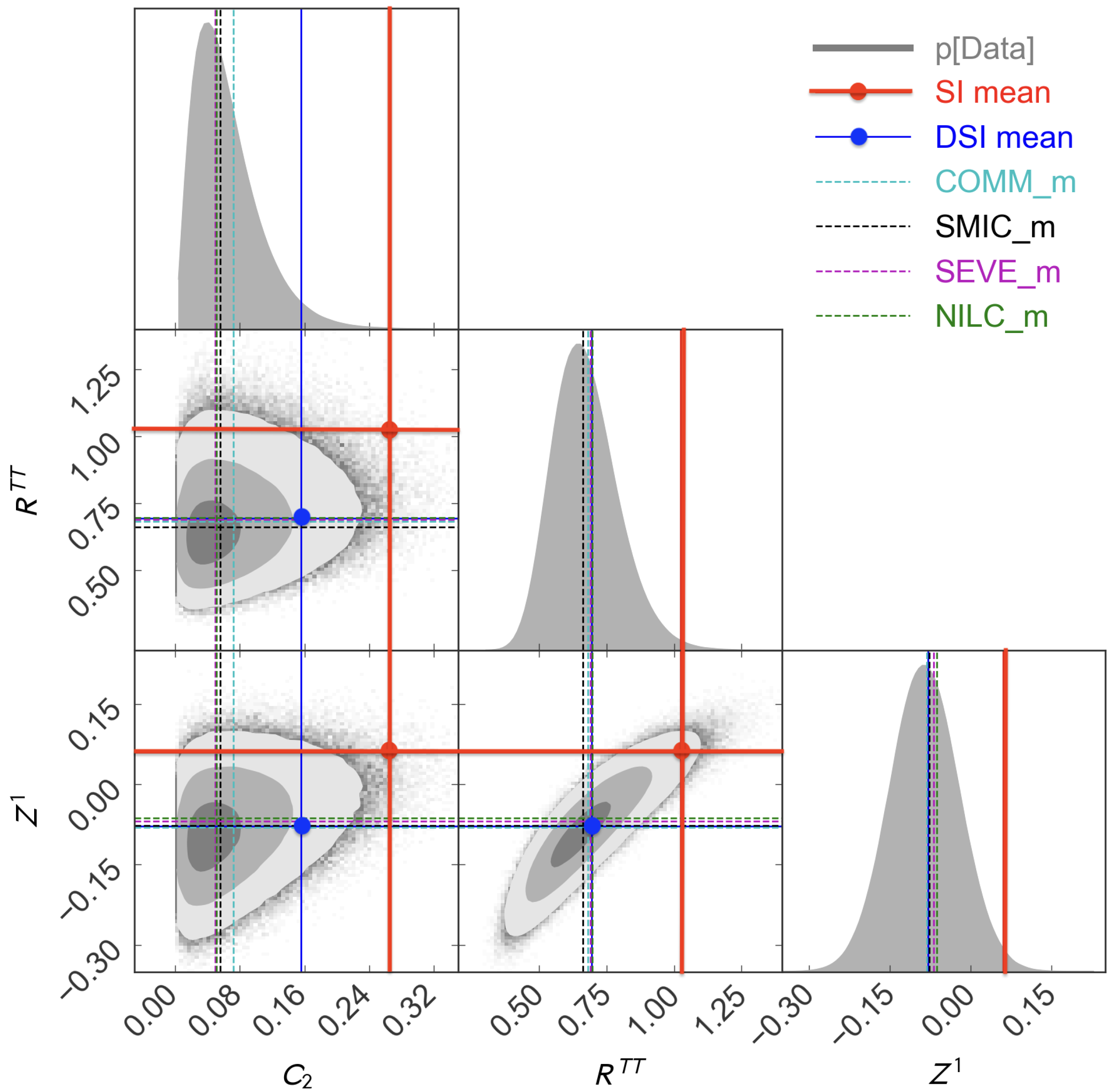
In Figure 5 we present how the observational data significantly prefer DSI over SI. Observed quantities include the observed low quadrupolar amplitude , the even-to-odd multipole ratio of angular power spectra:
and the mean of the parity map displayed in Figure 4, where represents the parity conjugate or antipode of the sky position . The likelihood probability associated with DSI in these plots is up to 650 times larger than that of SI. DSI favors odd parity, leading to a lower . This, in turn, diminishes the significance of other CMB anomalies ([27]), such as the Hemispherical Power Asymmetry, the axis of Evil, and the anomalous 2-point correlation function (see [8] for further details).
5. Conclusions
In this paper, we underscore the pivotal role of unitary Quantum Field Theory in Curved Spacetime (QFTCS) in elucidating the intricacies of early Universe physics. Contrary to prevailing notions, we contend that the issue of unitarity in QFTCS is not inherently tied to quantum gravity at Planck scales, but rather stems from throwing away the symmetry for quantum fields in curved spacetime.
With the -symmetric formulation of Schrödinger equation Eq.1, the DQFT framework reinstates unitarity, which was previously thought to be lost in curved spacetime. Figure 1and Figure 2 visually represent this concept, illustrating how a hypothetical classical observer consistently experiences pure states without encountering information loss beyond the horizon. Furthermore, the striking correlation illustrated in Figure 3, Figure 4 and Figure 5 between the observed hot and cold mirrored structures of the CMB map at antipodal points strongly supports the unitary treatment of inflationary quantum fluctuations within the framework of DQFT. Our findings indicate that superhorizon fluctuations at antipodes manifest as conjugates, a prediction derived from direct-sum QFTCS. This prediction is substantially favored with a probability over 650 times greater than that of the standard QTFCS.
Funding
EG acknowledges grants from Spain Plan Nacional (PGC2018-102021-B-100) and Maria de Maeztu (CEX2020-001058-M). KSK acknowledges the Royal Society for the Newton International Fellowship.
Data Availability Statement
No new data is presented.
Conflicts of Interest
The authors declare no conflict of interest.
Appendix A. Klein-Gordon Field Operator in DQFT
The Klein-Gordon field operator for DQFT in Minkowski spacetime split into direct-sum
where
where . The creation and annihilation operators satisfy the canonical relations
which defines the positive norm states in the direct-sum vacuums . The second condition in Eq.A3 implies commutativity of operators , which can be seen as a new causality condition. The The Fock space in DQFT is the direct-sum of two Fock spaces (geometric superselection sectors) corresponding to the components of field operators that lead to the quantum states forward and backward in time at parity conjugate regions of position space. These field operators are defined through the pairs of creation and annihilation operators Eq.A3. Since the Minkowski spacetime is symmetric, the scalar field operator in DQFT respects the same symmetry. Generalizing this structure to all quantum fields in Minkowski spacetime, such as complex scalar, vector, and fermionic degrees of freedom, is very straightforward. Any standard model (single particle) state, whether it is particle ( or anti-particle (, is expressed in DQFT as direct-sum of two components
with respect to conjugate splitting of the vacuum . For further details on DQFT in particular, the CPT invariance of scattering amplitudes which holds in both geometric superselection sectors, and quantizing other fields of the standard model, see [5].
Appendix B. DQFT in dS
Appendix C. DSI Angular Power Spectrum
Here, are the Hankel and Bessel functions of the first kind, and is the cut-scale we impose as Eq.A8 is accurate enough for low-ℓ or large angular scales. This cutoff scale is also related to the coarse-gaining scale of stochastic inflation ([8]), which determines the large wavelength modes that have already become classical on the onset of inflation while the mode exits the horizon. In DSI, these large-wavelength modes create parity asymmetric inhomogeneities that correct the FLRW spacetime on large scales. The parity asymmetry ceases to exist towards the small scales because the symmetry recovered towards the short distance scales. This can be seen in Fig. 11 of [8]. An intuitive explanation for this is that large wavelength modes experience quantum gravitational effects more than those of short wavelength modes. For the small scales , the predictions of DSI become almost the same as with the (near) scale-invariant power spectrum as contributions from term become negligible.
References
- Coleman, S. Lectures of Sidney Coleman on Quantum Field Theory; WSP: Hackensack, 2018. [Google Scholar] [CrossRef]
- Mukhanov, V.F.; Chibisov, G.V. Quantum Fluctuations and a Nonsingular Universe. JETP Lett. 1981, 33, 532–535. [Google Scholar]
- Sasaki, M. Large Scale Quantum Fluctuations in the Inflationary Universe. Prog. Theor. Phys. 1986, 76, 1036. [Google Scholar] [CrossRef]
- Albrecht, A.; Ferreira, P.; Joyce, M.; Prokopec, T. Inflation and squeezed quantum states. Phys. Rev. D 1994, 50, 4807–4820. [Google Scholar] [CrossRef] [PubMed]
- Kumar, K.S.; Marto, J.a. Towards a Unitary Formulation of Quantum Field Theory in Curved Spacetime: The Case of de Sitter Spacetime. Symmetry 2025, arXiv:hep-th/2305.06046]17, 29. [Google Scholar] [CrossRef]
- Kumar, K.S.; Marto, J. Towards a Unitary Formulation of Quantum Field Theory in Curved Space-Time: The Case of the Schwarzschild Black Hole. PTEP 2024, arXiv:hep-th/2307.10345]2024, 123E01. [Google Scholar] [CrossRef]
- Gaztañaga, E.; Kumar, K.S.; Marto, J. A New Understanding of Einstein-Rosen Bridges. Preprint, /: physics/https, 2024. [Google Scholar] [CrossRef]
- Gaztañaga, E.; Kumar, K.S. Finding origins of CMB anomalies in the inflationary quantum fluctuations. JCAP 2024, arXiv:astro-ph.CO/2401.08288]06, 001. [Google Scholar] [CrossRef]
- Donoghue, J.F.; Menezes, G. Arrow of Causality and Quantum Gravity. Phys. Rev. Lett. 2019, arXiv:hep-th/1908.04170]123, 171601. [Google Scholar] [CrossRef] [PubMed]
- Kiefer, C. Quantum Gravity, 2nd ed ed.; Oxford University Press: New York, 2007. [Google Scholar]
- Erwin Schrodinger. Expanding universes, Cambridge University Press, 1956.
- Gibbons, G.W.; Hawking, S.W. Cosmological Event Horizons, Thermodynamics, and Particle Creation. Phys. Rev. D 1977, 15, 2738–2751. [Google Scholar] [CrossRef]
- Parikh, M.K.; Savonije, I.; Verlinde, E.P. Elliptic de Sitter space: dS/Z(2). Phys. Rev. D 2003, 67, 064005. [Google Scholar] [CrossRef]
- Hawking, S.W. Black hole explosions? Nature 1974, 248, 30–31. [Google Scholar] [CrossRef]
- Wick, G.C.; Wightman, A.S.; Wigner, E.P. The intrinsic parity of elementary particles. Phys. Rev. 1952, 88, 101–105. [Google Scholar] [CrossRef]
- nLab authors. superselection theory. https://ncatlab.org/nlab/show/superselection+theory, 2023.
- Lanczos, K.; Hoenselaers, C. On a Stationary Cosmology in the Sense of Einstein’s Theory of Gravitation [1923]. GR and Gravitation 1997, 29, 361–399. [Google Scholar]
- Hartman, T. Lecture Notes on Classical de Sitter Space; 2017. http://www.hartmanhep.net/GR2017/desitter-lectures-v2.pdf.
- Mukhanov, V.; Winitzki, S. Introduction to quantum effects in gravity; Cambridge University Press, 2007.
- Gaztanaga, E. How the Big Bang Ends Up Inside a Black Hole. Universe 2022, 8, 257. [Google Scholar] [CrossRef]
- Gaztañaga, E. The mass of our observable Universe. MNRAS 2023, 521, L59–L63. [Google Scholar] [CrossRef]
- Gaztañaga, E.; Kumar, K.S.; Pradhan, S.; Gabler, M. Gravitational Bounce from the Quantum Exclusion Principle 2025. [CrossRef]
- Starobinsky, A.A. A New Type of Isotropic Cosmological Models Without Singularity. Phys. Lett. 1980, B91, 99–102. [Google Scholar] [CrossRef]
- Komatsu, E. New physics from the polarized light of the cosmic microwave background. Nature Rev. Phys. 2022, arXiv:astro-ph.CO/2202.13919]4, 452–469. [Google Scholar] [CrossRef]
- Akrami, Y.; et al. Planck 2018 results. VII. Isotropy and Statistics of the CMB. Astron. Astrophys. 2020, 641, A7. [Google Scholar] [CrossRef]
- Akrami, Y.; et al. Planck 2018 results. X. Constraints on inflation. Astron. Astrophys. 2020, arXiv:astro-ph.CO/1807.06211]641, A10. [Google Scholar] [CrossRef]
- Schwarz, D.J.; Copi, C.J.; Huterer, D.; Starkman, G.D. CMB Anomalies after Planck. Class. Quant. Grav. 2016, 33, 184001. [Google Scholar] [CrossRef]
Figure 1.
This figure depicts the concept of unitarity that can be novelly achieved in de Sitter spacetime (in flat FLRW coordinates) with DQFT. Given the particle horizon () at any moment of de Sitter expansion, the above picture depicts how the DQFT formulation projects all information of the states outside the horizon back inside at the antipodal point of the physical space. This implies that all the information that any imaginary classical observer perceives is within the horizon and that pure states evolve into pure states. Blue arrows indicate accessible from inside the horizon, while dashed lines indicate that in the quasi-deSitter case the time evolution of and could be different, which is the origin of creating CMB parity asymmetry in the large scales.
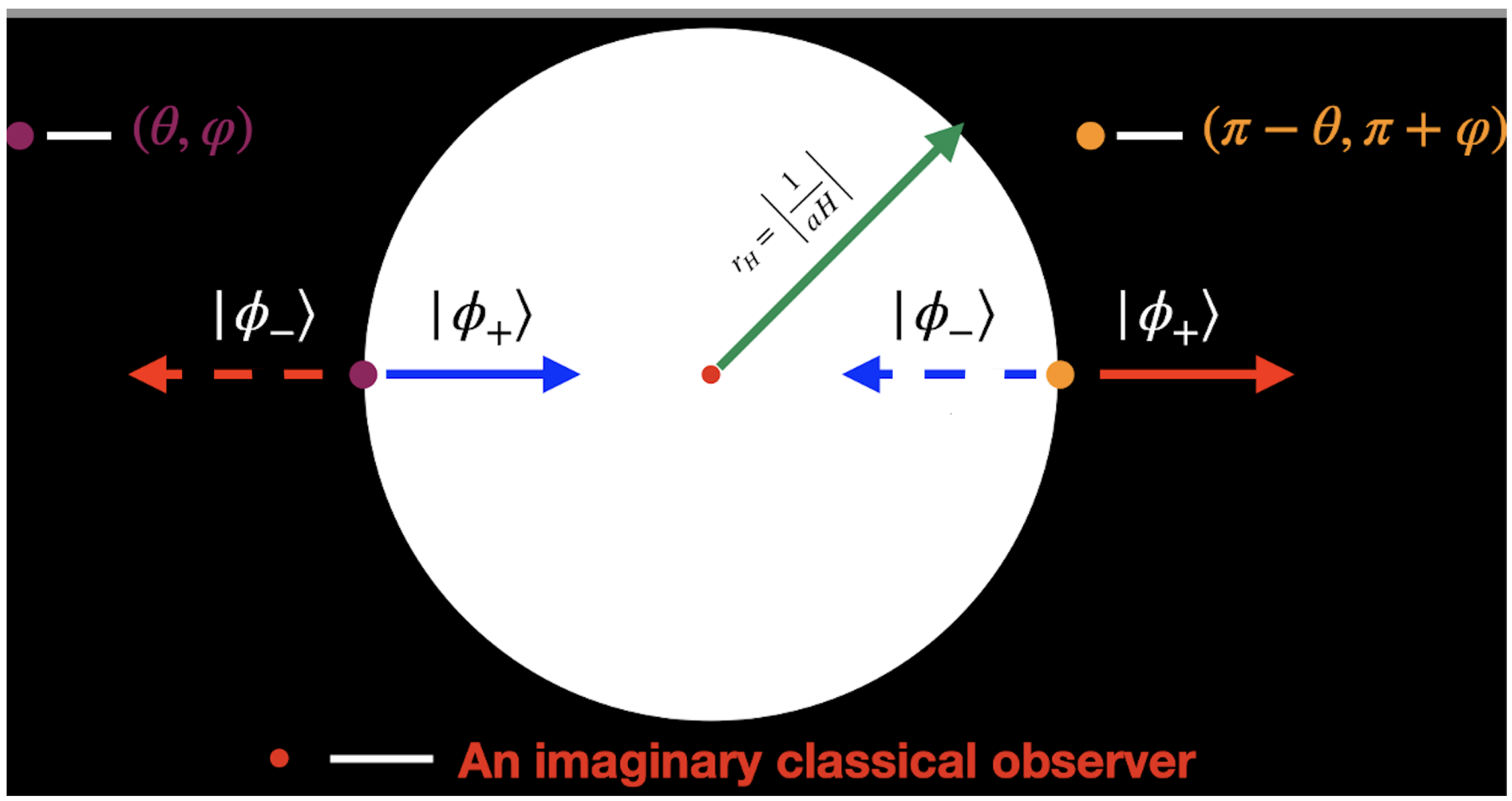
Figure 2.
This picture depicts the (quantum) conformal diagram of static dS spacetime Eq.12 with four regions that are related by discrete transformations and the lines with arrows indicate the arrows of time in each region. Here a quantum field operator is written as direct-sum of four components corresponding to the regions I to IV. This is not a Penrose diagram because each point represents half of the sphere in contrast to the usual Penrose diagram. This diagram is to represent quantum physics in dS space rather than classical physics for which the usual Penrose diagram is used.
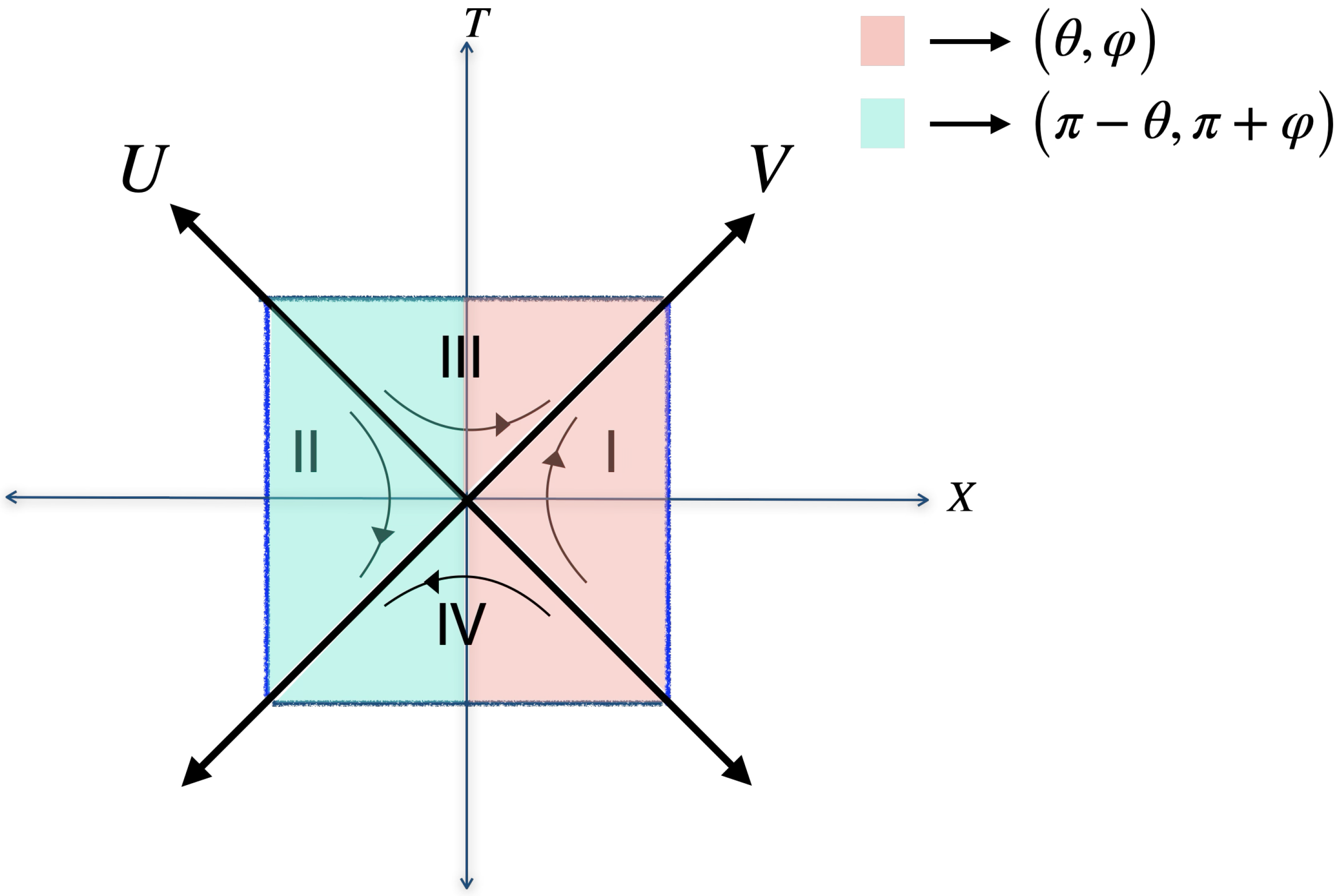
Figure 3.
The top panels show the anti-symmetric, , component of the Planck 2018 CMB temperature map ([25]) in North and South polar galactic caps. The visualization is such that the Galactic plane, shown in Figure 4, remains obscured along the edges. Parity conjugate positions can be identified by horizontally flipping into the opposite pole, where both caps have the same information with opposing signs: . The bottom panel presents the observed maps, including both the symmetric and anti-symmetric components. The evident resemblance between the top and bottom panels indicates the prevalence of the anti-symmetric component, in perfect agreement with DSI predictions Eq.A7.
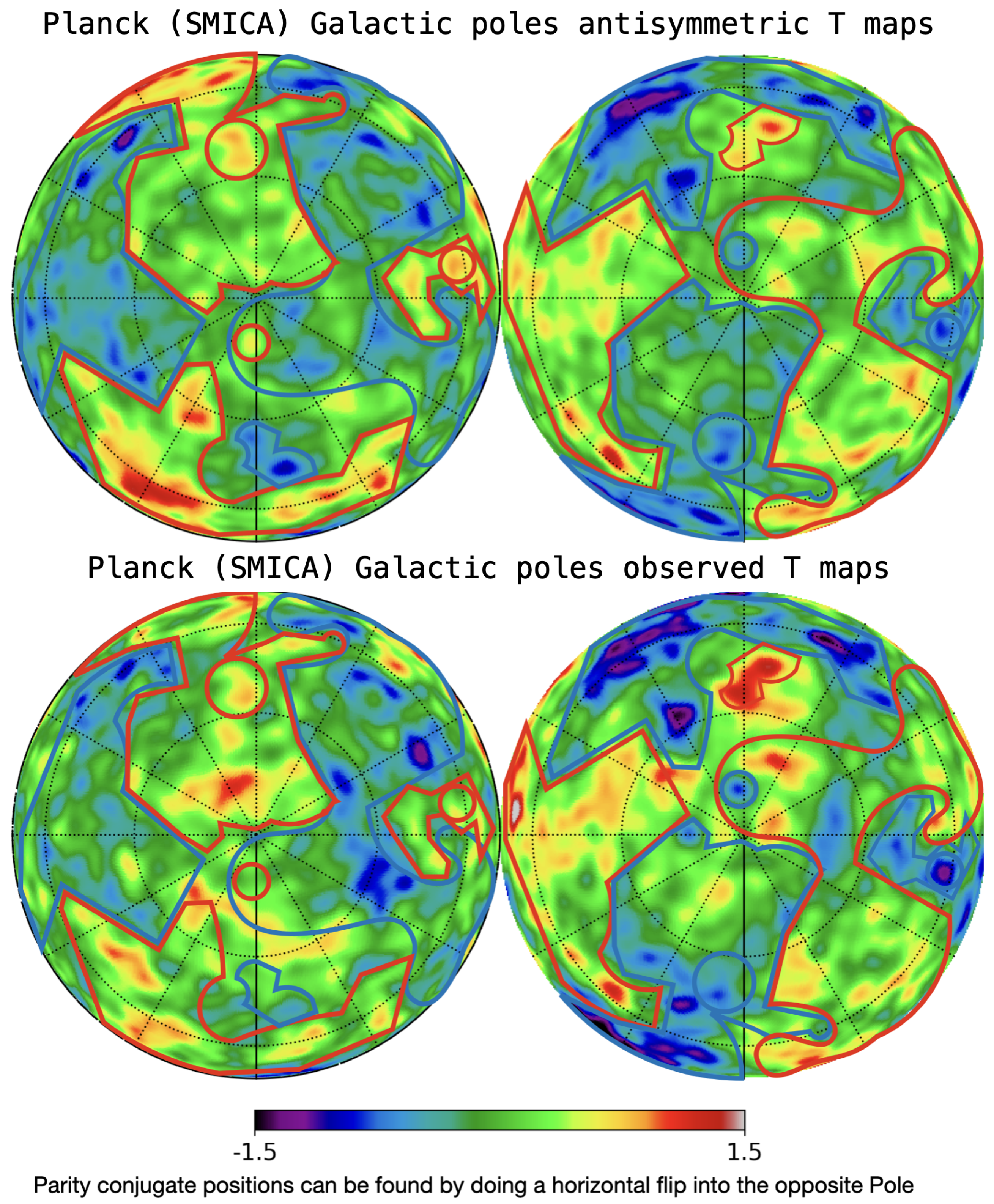
Figure 4.
Parity map: for Figure 3 with galactic mask. This is a conjugate image of itself. Positive values (red) correspond to the symmetric (even parity) component of , while negative values (blue) give the antisymmetric (odd parity) component. There is a clear excess of negative values, indicating a preference for odd parity. This, together with Figure 3 serves as a visual testament to the unitary QFTCS in nature.
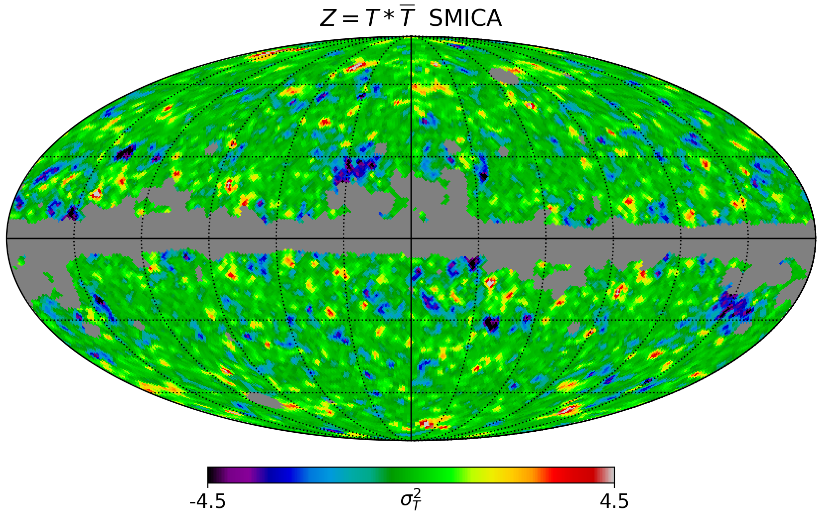
Figure 5.
Parity measurements derived from different mask (component separation) CMB temperature maps (dashed lines) against data simulations (grey areas represent 1, 2, and 3 sigma contours), alongside predictions from standard inflationary (SI) models (in red) and Direct-Sum inflation (DSI) (in blue). The later is 650 more probable.
Disclaimer/Publisher’s Note: The statements, opinions and data contained in all publications are solely those of the individual author(s) and contributor(s) and not of MDPI and/or the editor(s). MDPI and/or the editor(s) disclaim responsibility for any injury to people or property resulting from any ideas, methods, instructions or products referred to in the content. |
© 2025 by the authors. Licensee MDPI, Basel, Switzerland. This article is an open access article distributed under the terms and conditions of the Creative Commons Attribution (CC BY) license (http://creativecommons.org/licenses/by/4.0/).
Copyright: This open access article is published under a Creative Commons CC BY 4.0 license, which permit the free download, distribution, and reuse, provided that the author and preprint are cited in any reuse.


