
Submitted:
02 May 2025
Posted:
05 May 2025
You are already at the latest version
Abstract
Despite ongoing efforts to make black-box machine learning models more explainable, transparent, and trustworthy, there is growing advocacy for using only inherently interpretable models for high-stakes decision-making. Post-hoc explanations have been criticized for learning surrogate models that may not accurately reflect the actual mechanisms of the original model and for adding computational burden at prediction time. We propose two novel explainability approaches to address these limitations: pre-hoc explainability and co-hoc explainability. These approaches integrate explanations derived from an inherently interpretable white-box model into the learning stage of the black-box model without compromising accuracy. Unlike post-hoc methods, our approach does not rely on random input perturbation or post-hoc training alone. We extend our pre-hoc and co-hoc frameworks to generate instance-specific explanations by incorporating the Jensen-Shannon divergence as a regularization term while capturing the local behavior of the black-box model. This extension provides local explanations that are faithful to the model’s behavior and consistent with the explanations generated by the global explainer model. Our two-phase approach first trains models for fidelity, then generates local explanations by fine-tuning the explainer model within the neighborhood of the instance being explained. Experiments on three benchmark datasets from different domains (credit risk scoring and movie recommendations) demonstrate the advantages of our techniques in terms of global and local fidelity without compromising accuracy. Our methods avoid the pitfalls of surrogate modeling, making them more scalable, robust, and reliable compared to post-hoc techniques like LIME. Additionally, our co-hoc learning framework enhances the accuracy of white-box models by up to 3%, highlighting its potential for applications in healthcare and legal decision-making where interpretable models are required. Our approaches provide more faithful and consistent explanations at a lower computational cost than existing methods, offering a promising direction for making machine learning models more transparent and trustworthy while maintaining high prediction accuracy.
Keywords:
XAI
; Explainability in Machine Learning
; Local Explainability
; Global Explainability
1. Introduction
Machine learning models are increasingly used to support decision-making in various fields, from personalized medical diagnosis to credit risk assessment and criminal justice. However, the increasing reliance on powerful black-box models raises concerns about their transparency, interpretability, and trustworthiness [1,2,3]. Understanding why a model made a particular prediction is crucial for auditing models, detecting potential biases and errors, and supporting model accountability and fairness. Explainable Artificial Intelligence (XAI) has emerged as a new research area that focuses on machine learning interpretability. The goal is to build interpretable models that will generate high-performing machine learning predictions [4] and thus enable human users to understand the models and trust them. In machine learning, the term explainability still lacks a common meaning, and the capability varies from application to application. Interpretability is often used instead. However, traditionally, explainability or interpretability refers to the ability of an artificial intelligence system to be understood by humans [5].
Explainable AI helps build trust in machine learning systems by providing insights into how models make decisions. This is particularly important in high-stakes domains such as healthcare, finance, and criminal justice, where the consequences of incorrect or biased decisions can be severe. When users understand how a model arrives at a particular output, they are more likely to trust and rely on the system [6,7]. Explanations can help identify errors, biases, and unexpected behaviors in machine learning models. Developers can debug and improve their models by understanding how features influence predictions, leading to more accurate and reliable systems [8,9]. In some domains, there are legal and regulatory requirements to explain algorithmic decisions. For example, the European Union’s General Data Protection Regulation (GDPR) includes a “right to explanation" for individuals subject to automated decision-making. Explainable AI techniques can help organizations comply with these regulations [10,11]. Explainable AI can also help uncover biases and unfairness in machine learning models [12,13]. Furthermore, explainable AI enables effective human-AI collaboration by providing a common understanding between humans and machines [14,15].
Several approaches have been proposed to explain black-box models, ranging from local methods that provide explanations for individual predictions to global methods that aim to capture the model’s overall behavior. Post-hoc explanations, such as LIME (Local Interpretable Model-Agnostic Explanations) [16], SHAP (Shapley Additive Explanations) [17], and Grad-CAM (Gradient Weighted Class Activation Mapping) [18], have gained popularity in recent years as a way to explain black-box models by perturbing the input data and learning a surrogate model that approximates the original model’s behavior locally. Although these methods can effectively generate explanations, they have been criticized for several reasons. First, the explanations may not reflect the true mechanisms of the original model but rather a simplified version that is easier to interpret [19]. Second, the surrogate model may not be faithful to the behavior of the original model in some cases, leading to potentially misleading explanations and being open to adversarial attacks [20]. Third, the perturbation of input data can alter the features’ semantics, rendering the explanations invalid or misleading and creating unstable explanations that arise with models already trained [21,22].
To address these limitations, some researchers have proposed using inherently interpretable models, such as decision trees or linear models, instead of black-box models for high-stakes decision-making [23]. However, this approach may come at the cost of reduced prediction accuracy, as interpretable models may not be able to capture the complexity of some datasets as well as black-box models. Moreover, this approach cannot be applied to models that are already deployed and running. Replacing existing black-box models in production with interpretable models requires re-training the whole model from scratch, which can be resource-intensive and time-consuming.
We propose two novel approaches to improving the explainability of black-box models, which we call pre-hoc explainability and co-hoc explainability. Our approach aims to incorporate explanations derived from an inherently interpretable white-box model into the original model’s learning stage without compromising its high prediction accuracy. Instead of learning a post-hoc white-box model, our idea is to learn a white-box model that is explainable from the start and then let this explainer model guide the learning of the black-box predictor model. This approach aims to address the limitations of post-hoc explanations, such as potential discrepancies between the explainer and the black-box model [24], and the computational overhead associated with generating explanations after model training [20].
To accomplish this goal, we design two different frameworks: (1) A Pre-Hoc Explainable Predictive Framework, where the white-box model regularizes the black-box model for optimized fidelity, and (2) A Co-hoc Explainable Predictive Framework, where the white-box and black-box models are optimized simultaneously with a shared loss function that enforces fidelity.
In the Pre-Hoc Explainable Predictive Framework, we first train the explainer model g and then use it to guide the learning of the predictor model f. The objective function for training the predictor model includes a fidelity term that minimizes the distance between the predictor’s and explainer’s outputs, encouraging the predictor to mimic the explainer’s behavior. This approach ensures that the predictor model is regularized by the explainer model, leading to improved interpretability.
In the Co-hoc Explainability Framework, we jointly optimize the predictor model f and the explainer model g during training. The shared loss function consists of both models’ standard supervised learning objective (e.g., cross-entropy loss) and a fidelity term that minimizes the distance between their outputs. By simultaneously training both models, we encourage the predictor to learn from the explainer and the explainer to adapt to the predictor, resulting in a more coherent and interpretable system.
Our proposed frameworks differ from existing approaches in several aspects. First, we integrate interpretability directly into the model training process rather than relying on post-hoc explanations. Second, we use a transparent white-box model to guide the learning of the black-box model, ensuring that the explanations are faithful to the predictor’s behavior. Finally, our frameworks are model-agnostic and can be applied to any differentiable predictor and explainer models.
The main contributions of this paper are:
- We propose two novel approaches to improving the explainability of black-box models, called pre-hoc explainability and co-hoc explainability, which leverage the insights provided by an inherently interpretable white-box model to guide the training of the black-box model in a way that preserves its accuracy while enhancing its global interpretability. These approaches integrate explainability directly into the training process, ensuring that the explanations are faithful to the model’s behavior and do not require additional post-hoc computations.
- We extend our pre-hoc explainability framework to provide local explanations by incorporating the Jensen-Shannon (JS) divergence [25] as a regularization term in the loss function. This allows our method to generate instance-specific explanations that capture the local behavior of the black-box model, similar to post-hoc methods such as LIME [16]. However, unlike LIME, our approach integrates local explainability directly into the training process, ensuring that the explanations are faithful to the model’s behavior and consistent with the model’s predictions for similar instances.
- Unlike post-hoc explanations, our approaches do not rely on random input perturbation and post-secondary model learning, thus avoiding the potential pitfalls of surrogate modeling, such as instability and unfaithfulness [20,26]. This makes them more scalable, robust, and reliable in practice. By incorporating global and local explainability through an interpretable white-box model and the JS divergence, our methods can generate more accurate and stable explanations compared to LIME.
- We enhance the accuracy of white-box models through the co-hoc learning framework. The white-box model, which is learned for the purpose of explaining the black-box predictor, achieves significantly higher prediction accuracy after the co-hoc learning process. This finding highlights the potential of the co-hoc in-training approach to improve the performance of white-box models, which are essential and required in certain high-risk and regulated application tasks in healthcare and legal decision-making.
- We demonstrate the effectiveness of our approaches on three benchmark datasets from diverse domains (credit risk scoring and movie recommendations), showing that they outperform traditional black-box models in terms of fidelity while maintaining comparable accuracy. We also compare our methods with the LIME post-hoc explainability technique [16] in terms of the quality and stability of the generated explanations, as well as the computational cost associated with generating explanations.
The remainder of this paper is organized as follows: Section 2 reviews related work in explainable artificial intelligence. Section 3 presents our proposed pre-hoc and co-hoc explainability frameworks and their theoretical foundation and describes our experimental setup and evaluation metrics. Section 4 presents and discusses the results of our experiments. Finally, Section 5 concludes the paper and outlines potential future research directions.
2. Related Work
2.1. Explainability Approaches in Machine Learning
The landscape of explainable artificial intelligence (XAI) encompasses several distinct approaches. Inherently interpretable models, such as linear models [27,28] and decision trees [29,30], offer transparent decision-making processes at the potential cost of reduced predictive power. While these white-box models provide clarity, they often cannot match the performance of complex black-box models in challenging tasks [23].
Post-hoc explainability techniques aim to explain already-trained black-box models. LIME (Local Interpretable Model-Agnostic Explanations) [16] approximates complex models locally around specific predictions using simpler, interpretable surrogate models. LIME solves the optimization problem:
where represents a regularizer that encourages desirable properties like sparsity. Similarly, SHAP (SHapley Additive exPlanations) [17] applies game theory concepts to assign feature importance values. Despite their popularity, these approaches have been criticized for generating potentially misleading or unstable explanations [20,26] and introducing computational overhead during inference [19].
Model-specific explainability techniques, or explainability by design, involve architectural adjustments to improve model interpretability. These approaches modify model architecture to enhance comprehensibility [31,32,33,34] and often employ regularization techniques to promote sparsity and interpretability [35,36].
2.2. In-Training Explainability Techniques
While most XAI research has focused on post-hoc explainability or inherently interpretable models, in-training explainability represents a less explored but promising direction. Tree regularization [37] has been used to train deep time-series models with a focus on human-simulability [38]. Others have proposed training models with latent explainability but still rely on post-hoc explanations [39,40].
Alternative approaches include game-theoretic methods between predictor and explainer [41,42], using cooperative games to optimize explainers for locality. The EXPO framework [43] applied regularization to push black-box models toward interpretable features, but their explanations remain post-hoc, specifically optimized for LIME’s neighborhood-based fidelity, which requires computation at prediction time. Concept-based explanation methods [44] learn latent explanations during training but are limited to special input types or domains with available external supervision.
Current research highlights the need for optimization during training and model-agnostic methods to improve global explainability. Our approach addresses this gap by directly incorporating global interpretability into black-box learning at training time through an interpretable explainer model that doesn’t require additional post-hoc computation at prediction time.
2.3. Explanation Types and Evaluation
XAI explanations can be categorized into several types, each offering different perspectives and serving distinct purposes. Rule-based explanations transform model decisions into human-readable rules, making them particularly valuable in domains requiring transparency, such as healthcare and finance [45,46]. Decision trees exemplify this approach by breaking decisions into comprehensible if-then rules. While intuitive, these explanations may become unwieldy as model complexity increases.
Feature-based explanations quantify the contribution of individual features to predictions [16,47]. LIME and SHAP are prominent techniques in this category, with LIME approximating local behavior using interpretable models and SHAP assigning feature importance based on game theory principles. These methods provide valuable insights into which inputs most strongly influence outputs, enabling feature selection and bias detection. However, they may not capture complex feature interactions or non-linear relationships effectively [48].
Concept-based explanations bridge the gap between model internals and human understanding by expressing decisions through high-level concepts [49,50]. Techniques like Concept Activation Vectors (CAVs) align model behavior with human-understandable concepts, which is particularly useful in domains with established conceptual frameworks like medicine. These explanations facilitate communication with domain experts but require well-defined concepts and may not capture the model’s full complexity.
Instance-based explanations identify specific training examples that significantly influence predictions [8,51]. Techniques like influence functions measure how individual training instances affect model outputs, while prototype selection identifies representative examples that characterize decision boundaries. These concrete explanations help users understand model behavior through familiar examples, though interpretation can be challenging when influential instances aren’t intuitively related to predictions.
Local explanations focus on individual predictions, explaining specific decisions rather than overall model behavior [16,47]. These targeted insights are crucial in domains where individual decisions carry significant consequences. Conversely, global explanations describe the model’s general behavior across all instances [45,52], providing a holistic understanding of the model’s decision logic through interpretable surrogate models or feature importance methods.
Multi-model explanations generate comparative views across different models [53,54], helping users understand similarities and differences in how various models process information. This comparative approach provides insights into model robustness and generalizability, but can be computationally expensive and challenging to reconcile when models yield conflicting explanations.
Selecting appropriate explanation types depends on factors including the target audience, model complexity, and application domain. In healthcare, concept-based explanations may better communicate with medical professionals, while rule-based explanations might be more suitable for patient-facing applications [55]. Different explanation types can be combined for comprehensive understanding—for example, aggregating local explanations to generate global insights [56].
Post-hoc explainability can be evaluated using three key metrics: point fidelity, neighborhood fidelity [43], and stability [26]. Point fidelity measures agreement between the explainer and predictor for individual instances:
The average point fidelity across all instances is calculated as:
Neighborhood fidelity extends this concept to consider agreement within local neighborhoods around each instance, providing a more robust measure of explanation quality:
where denotes the set of k-nearest neighbors of instance in the feature space. This metric assesses how well explanations generalize to similar instances, capturing the local coherence of explanations.
The stability metric quantifies the variability in fidelity scores using total variation:
where represents a set of fidelity scores. Lower total variation indicates higher stability, suggesting that explanations remain consistent across different instances without sudden fluctuations. Stability is crucial for building trust in explanations, as users expect similar explanations for similar instances.
These evaluation metrics provide complementary perspectives on explanation quality. Point fidelity focuses on individual accuracy, neighborhood fidelity considers local coherence, and stability measures consistency across instances. A desirable explainable model would achieve high average fidelity scores and low total variation, indicating explanations that are both accurate and stable across different instances. Together, these metrics offer a comprehensive framework for assessing explanation quality that aligns with the multifaceted nature of interpretability [5,57].
2.4. Factorization Machines
Factorization Machines (FMs) [58] are supervised learning models applicable to various prediction tasks including regression, classification, and ranking. The model equation for a degree-2 FM is:
Despite their effectiveness, FMs lack transparency. The model parameters () include latent factors that make interpretability challenging. Recent efforts to improve FM transparency include Subspace Encoding Factorization Machines (SEFM) [59], Knowledge-aware Hybrid Factorization Machines (kaHFM) [60], and Attentional Factorization Machines (AFM) [61].
Our proposed pre-hoc and co-hoc explainability frameworks address the limitations of both post-hoc techniques and inherently interpretable models by integrating explainability directly into the training process of black-box models, ensuring faithful explanations without compromising accuracy.
3. Methodology
3.1. Problem Formulation
Let be a sample from a distribution in a domain , where is the instance space and is the label space. We learn a differentiable predictive function together with a transparent explainer function defined over a functional class . We refer to functions f and g as the predictor and the explainer, respectively, throughout the paper. is strictly constrained to be an inherently explainable functional set, such as a set of linear functions or decision trees. We assume that we have a distance function such that , which measures the point-wise similarity between two probability distributions in and can be used to optimize f and g.
Instead of learning a post-hoc white-box model, our idea is to learn a white-box model that is explainable from the start and then let this explainer model guide the learning of the black-box predictor model. To accomplish this goal, we design two different frameworks: (1) A Pre-Hoc Explainable Predictive Framework, where the white-box model regularizes the black-box model for optimized fidelity, and (2) A Co-hoc Explainable Predictive Framework, where the white-box and black-box models are optimized simultaneously with a shared loss function that enforces fidelity.
3.1.1. Enforcing Fidelity
Given an inherently interpretable white-box model g with parameters , let its predictions result in a probability distribution . Given the black-box model f with parameters , let its predictions result in probability distribution over K classes . We propose a fidelity objective function, which measures the point-wise probability distance between and , which are respectively the outputs of g and f for all given input data . The optimization problem is formulated as:
where function D is a divergence distance measurement, such as the Jensen-Shannon divergence [62]. We use , Jensen-Shannon divergence, to measure the point-wise deviation of the predictive distributions and .
Denote by the set of probability distributions. The Kullback-Leibler divergence (KL). KL : is a fundamental distance between probability distributions in [63], defined by:
where p and q denote probability measures P and Q with respect to .
Let have the corresponding weights . Then, the Jensen-Shannon divergence between p and q is given by:
with H the Shannon entropy, and . Unlike the Kullback-Leibler divergence , JS is symmetric, bounded, and does not require absolute continuity.
We propose a fidelity objective function, , that is calculated using the Jensen-Shannon divergence (JS), as follows:
Our proposed fidelity objective function has three distinct regularization properties:
Bounded Regularizer: The Jensen–Shannon divergence distance is always bounded:
Symmetry Preserving Regularizer: JS is symmetry preserving if the corresponding weights are selected as .
Differentiable Regularizer: The regularizer is differentiable, which means that it can be easily incorporated into the training process using standard gradient descent update rules and backpropagation techniques.
3.2. Pre-hoc Explainability Framework
The Pre-hoc Explainability Framework uses a modified learning objective to incorporate explanations during the training process. In this framework, we first train a white-box explainer model on the training data. Then, we use this explainer model to guide the learning of the black-box predictor model by including a fidelity term in the loss function.
The loss function for the Pre-hoc framework is formulated as:
where is the binary cross-entropy loss that ensures accurate predictions, is an explainability regularization coefficient that controls the trade-off between explainability and accuracy, and is the coefficient for standard regularization of model parameters that aims to avoid overfitting and exploding gradients.
Expanding the loss function, we get:
Since the explanation is provided by the white-box model that is inherently interpretable, the transparency is considered high when the explainer model outputs are similar to the regularized model outputs . This similarity is captured by , which is the Fidelity term in the objective function (Eq. 13). While the objective function is to learn a model that will make accurate predictions, we give greater importance to model predictions that are similar to the white-box predictions and penalize those that are not similar.
The optimization procedure for the Pre-hoc framework is as follows:
- Train the white-box explainer model on the training data to minimize the binary cross-entropy loss.
- Fix the parameters of the explainer model.
- Train the black-box predictor model to minimize the combined loss function .
3.3. Co-Hoc Explainability Framework
In contrast to the Pre-hoc framework, the Co-hoc Explainability Framework jointly optimizes both the predictor model and the explainer model during training. This approach allows the explainer to adapt to the predictor and vice versa, resulting in a more coherent and interpretable system.
The loss function for the Co-hoc framework is given by:
The primary distinction between the Co-hoc and Pre-hoc frameworks lies in the joint optimization of the predictor and explainer through simultaneous stochastic gradient descent with mini-batches. In the Co-hoc framework, both models are trained to minimize the combined loss function , which includes accuracy terms for both models, a fidelity term, and regularization terms.
The optimization procedure for the Co-hoc framework is as follows:
- (1)
- Initialize the parameters of the predictor model and of the explainer model.
- (2)
-
For each mini-batch of training data:
- (a)
- Compute the predictions of both models: and .
- (b)
- Calculate the combined loss function .
- (c)
- Update both sets of parameters and using gradient descent.
3.4. Generating Explanations
Once the models are trained, the white-box explainer model naturally provides interpretable explanations for the predictions made by the black-box model . For linear models, the feature importance scores can be directly derived from the model coefficients, providing a global understanding of feature relevance across the entire dataset.
For a specific instance, we generate feature importance scores based on the trained white-box model and the feature values. The importance score of feature j for instance i is calculated as:
where is the coefficient of feature j in the trained white-box model, and is the mean absolute deviation of feature j across the dataset, calculated as:
where is the value of feature j for instance i, and is the mean value of feature j across all instances.
The mean absolute deviation serves as a scaling factor to normalize feature importance scores, ensuring that the scores are comparable across different features and datasets. By incorporating the MAD in the importance score calculation, we account for the variability and scale of the features, providing a more reliable and interpretable measure of feature importance.
3.5. Extending to Local Explainability
While the frameworks described above provide global explanations that capture the overall behavior of the black-box model, they may not adequately explain individual predictions. To address this limitation, we extend our pre-hoc and co-hoc frameworks to incorporate local explainability, enabling the generation of instance-specific explanations.
3.5.1. Local Explainability with Neighborhood Information
Local explainability refers to understanding and interpreting a model’s predictions at an individual instance level. We leverage neighborhood information and the Jensen-Shannon divergence to achieve local explainability. By considering each instance’s local neighborhood and comparing the predictions of the black-box model with those of the white-box model within this neighborhood, we can capture the regional variations in predictions and ensure that the explanations are faithful to the model’s local behavior.
We define the neighborhood fidelity objective function as follows:
where denotes the set of instances in the local neighborhood of instance , and is a divergence measure such as the Jensen-Shannon divergence computed over the neighborhood.
The Jensen-Shannon divergence for local explainability is given by:
3.5.2. Two-Phase Approach for Local Explainability
Our approach to local explainability consists of two phases: Phase 1: Co-hoc: Integrating Local Explainability with Neighbors in Training. In the first phase, we train the black-box predictor and white-box explainer models using our pre-hoc or co-hoc frameworks, incorporating the local neighborhood information. The loss functions are modified to include the local Jensen-Shannon divergence:
For the Pre-hoc Local Explainability framework:
For the Co-hoc Local Explainability framework:
Phase 2: Computing Local Explanations. In the second phase, for each test instance , we identify its nearest neighbors from the training set, forming a local in-testing neighborhood . We then fine-tune the global white-box explainer model within this neighborhood to obtain a local explainer model . The fine-tuning is performed by minimizing:
| Algorithm 1:Testing PHASE 2: Computing Local Explanations |
 |
This fine-tuned local explainer model provides instance-specific explanations that capture the local behavior of the black-box model around the test instance. The feature importance scores are then extracted from the local explainer model, quantifying the contribution of each feature to the model’s prediction for that specific instance.
3.6. Experimental Setup
3.6.1. Datasets
We evaluate our frameworks on three publicly accessible real-world datasets:
HELOC Dataset: The FICO HELOC dataset [64] contains 10,459 anonymized records of home equity line of credit applications. The target variable predicts whether an applicant will make payments on time.
MovieLens 100k: This dataset [65] contains 100,000 movie ratings from 1,000 users on 1,700 movies. We convert the ratings into a binary classification task, with ratings considered positive (1) and ratings considered negative (0).
MovieLens 1M: This dataset [66] contains movie ratings, has 1 million ratings based on 6000 users on 4000 movies. We convert the ratings into a binary classification task, with ratings considered positive (1) and ratings considered negative (0).
3.6.2. Evaluation Metrics
We use the following metrics to evaluate our frameworks:
Accuracy: We measure prediction accuracy using the Area Under the ROC Curve (AUC).
Fidelity: We measure how well the white-box explainer model mimics the behavior of the black-box predictor model using AUC.
Point Fidelity: This measures the agreement between the explainer and predictor for individual instances:
Neighborhood Fidelity: This extends point fidelity to consider agreement within local neighborhoods:
Stability: This measures the consistency of explanations, calculated as the total variation of fidelity scores:
Computational Efficiency: We measure the computational cost of generating explanations, including training time and explanation generation time.
3.6.3. Implementation Details
We implement our frameworks using PyTorch [67]. All models are trained using the Adam optimizer [68] with a learning rate of 0.001. Each dataset is split into training, validation, and test sets in the ratio 80:10:10. We select the optimal regularization parameter from the set {0.01, 0.05, 0.25, 0.5, 1} based on validation performance. For local explainability, we set the neighborhood size to k=10 during Phase 1 and k=100 during Phase 2. All experiments are repeated five times, and the results are averaged across runs.
As our black-box model, we use Factorization Machines [69], which are widely used for classification, regression, and recommendation tasks. For the white-box explainer model, we use sparse logistic regression, which is inherently interpretable and provides feature importance scores directly from its coefficients.
4. Results
In this section, we present the experimental results of our proposed pre-hoc and co-hoc explainability frameworks. We first examine the accuracy and fidelity trade-off of our global explainability approaches. Then, we analyze the local explainability performance and compare our approaches with the state-of-the-art post-hoc explainability method LIME.
4.1. Global Explainability Results
4.1.1. Accuracy and Fidelity Trade-off
Table 1 presents the accuracy (AUC) and fidelity scores of our pre-hoc and co-hoc frameworks compared to the baseline white-box (WB) and black-box (BB) models. We observe that both of our proposed frameworks achieve higher fidelity scores than the original black-box model while maintaining comparable accuracy. The co-hoc framework consistently outperforms the pre-hoc framework in terms of fidelity across all datasets, demonstrating the effectiveness of joint optimization.
The results confirm that our proposed approaches successfully maintain high accuracy while significantly improving fidelity. Notably, the co-hoc framework achieves fidelity improvements of 10.9%, 6.8%, and 10.9% on ML-100k, ML-1M, and HELOC datasets, respectively, compared to the original black-box model. This demonstrates the effectiveness of our joint optimization approach in aligning the behaviors of the black-box predictor and white-box explainer models.
4.1.2. Effect of Regularization Parameter
Figure 1 and Figure 2 illustrate the effect of the explainability regularization parameter on the precision and fidelity of our frameworks. As increases, we observe a consistent improvement in fidelity scores across all datasets, with only minimal impact on accuracy. This confirms that our frameworks effectively balance the trade-off between accuracy and explainability, allowing users to control this balance through the regularization parameter.
For example, the ML-100k dataset with the pre-hoc framework, as increases from 0.01 to 1.0, fidelity improves from 0.8207 to 0.9410 (a 14.6% increase), while accuracy remains relatively stable (0.7840 to 0.7740). Similarly, for the HELOC dataset, fidelity improves from 0.7482 to 0.8454 (a 9.3% increase) as increases, with accuracy actually improving slightly from 0.7591 to 0.7719. These results demonstrate that our frameworks can achieve high fidelity without sacrificing accuracy.
The co-hoc framework exhibits an even more favorable trade-off curve, particularly in the HELOC dataset, where both accuracy and fidelity improve simultaneously as increases. This suggests that the joint optimization approach not only aligns the behavior of the two models but also enhances their complementary strengths. The plateau observed in fidelity scores at higher values (above 0.5) indicates an optimal operating point beyond which additional regularization yields diminishing returns. This behavior provides practical guidance for hyperparameter selection in real-world applications, where setting between 0.25 and 0.5 offers the best balance between model performance and interpretability.
4.2. Local Explainability Results
4.2.1. Comparison with LIME
Table 2 presents the comparison of our local explainability frameworks with LIME on the HELOC in terms of point fidelity, neighborhood fidelity, and stability. Both our pre-hoc and co-hoc local explainability frameworks significantly outperform LIME across all metrics.
On the HELOC dataset, our frameworks achieve neighborhood fidelity scores of 0.9587 (pre-hoc) and 0.9647 (co-hoc), significantly higher than LIME’s score of 0.6600. Similarly, on the ML-100k dataset, our frameworks achieve neighborhood fidelity scores of 0.9597 (pre-hoc) and 0.9647 (co-hoc), outperforming LIME’s score of 0.7410. The stability of our explanations, measured by total variation, is also significantly better than LIME, indicating more consistent explanations across different instances.
4.3. Effect of Regularization Parameter on Local Explainability Metrics
Table 3 and Figure 3 shows the impact of the explainability regularization parameter on the point fidelity, neighborhood fidelity, and stability metrics for the Pre-hoc framework on the ML-100k dataset. The results show a clear positive relationship between the regularization strength and the quality of the explanation.
In the absence of regularization, the model achieves moderate fidelity scores (point fidelity of 0.8183 and neighborhood fidelity of 0.8050) but exhibits lower stability with a high total variation score of 0.3524. This indicates that without explainability regularization, the explanations are less consistent across different instances, even when the model achieves reasonable alignment with the explainer.
As we train with regularization parameter and gradually increase the , we observe significant improvements across all metrics. With a minimal regularization of , point fidelity improves to 0.8473 (3.5% increase), neighborhood fidelity increases to 0.8553 (6.2% increase), and stability improves dramatically with total variation decreasing to 0.1290 (63.4% reduction). At , point fidelity reaches 0.9740 (19.0% increase from no regularization), neighborhood fidelity increases to 0.9903 (23.0% increase), and stability improves substantially with total variation reduced to 0.0189 (94.6% reduction). This indicates that moderate regularization significantly enhances both the alignment between the predictor and explainer models and the consistency of explanations across different instances.
At higher regularization strengths ( and ), the metrics continue to improve but with decreasing returns. The point fidelity reaches its peak at 0.9951 with , representing a 21.6% improvement over the non-regularized model. Similarly, neighborhood fidelity reaches 0.9953, a 23.6% improvement. The stability metric plateaus at 0.0078 for both and , indicating that additional regularization beyond does not further improve the consistency of explanations.
These results demonstrate that incorporating explainability regularization through the Jensen-Shannon divergence significantly enhances the quality of explanations generated by the Pre-hoc framework. Even regularization provides substantial benefits, with optimal performance achieved at moderate to high regularization strengths (). The improvements in fidelity metrics indicate better alignment between the predictor and explainer models, while the reduction in total variation demonstrates more consistent explanations across different instances.
4.3.1. Effect of Neighborhood Size
Table 4 shows the effect of neighborhood size on neighborhood fidelity, stability, and computation time for the pre-hoc framework on the HELOC dataset. As the neighborhood size increases from 3 to 100, neighborhood fidelity improves from 0.8833 to 0.9670, and stability improves from 0.2152 to 0.0015, with only a minimal increase in computation time. This indicates that larger neighborhoods provide more stable and faithful explanations.
4.3.2. Computational Efficiency
Table 5 compares the computational efficiency of our frameworks with LIME on the HELOC dataset. Although our frameworks include an additional training phase, the average time to generate explanations for individual instances is significantly lower than LIME (0.011s vs. 0.3812s). This efficiency advantage becomes more apparent when generating explanations for multiple instances, with our frameworks being over 20 times faster than LIME for explaining 100 instances.
The computational efficiency of our frameworks is particularly advantageous in scenarios where real-time explanations are required or where a large number of instances need to be explained.
4.4. Qualitative Analysis of Explanations
4.4.1. Global Explanations
Figure 4 illustrates the global feature importance scores for the HELOC dataset, providing insights into the overall impact of each feature on the model’s predictions. The most influential feature is MaxDelq2PublicRecLast12M, which measures the maximum delinquency on public records in the last 12 months. This feature negatively impacts credit scores, suggesting that higher delinquency values significantly decrease the likelihood of getting a loan. Similarly, NumTrades90Ever2DerogPubRec, which represents the number of trades with derogatory public records, shows a substantial negative influence on the model’s predictions. This implies that having more trades with derogatory records decreases the probability of the target variable. The global explanation also reveals that features related to credit inquiries and satisfactory trades play a notable role in the model’s decision-making process. MSinceMostRecentInqexcl7days, indicating the time since the most recent credit inquiry, has a positive impact on the predictions, while NumSatisfactoryTrades, which represents the number of satisfactory trades, exhibits a negative influence. This suggests that recent credit inquiries and fewer satisfactory trades are associated with a higher likelihood of the target outcome.
4.4.2. Local Explanations
Figure 5 presents an example of local feature importance scores for a specific test instance from the HELOC dataset. The most influential feature for this instance is MSinceMostRecentInqexcl7days, which has a strong positive impact, indicating that a longer time since the most recent credit inquiry increases the likelihood of the target outcome for this specific instance.
Comparing the local explanation with the global explanation reveals interesting differences. Although both explanations highlight the importance of features such as MaxDelq2PublicRecLast12M and MSinceMostRecentInqexcl7days, the local explanation emphasizes features specific to the instance, such as PercentInstallTrades and NetFractionRevolvingBurden, which may not be as prominent in the global explanation. This shows the value of local explanations in capturing instance-specific factors influencing predictions.
4.5. Discussion
Our experimental results demonstrate that both the pre-hoc and co-hoc explainability frameworks outperform traditional post-hoc methods like LIME in terms of fidelity, stability, and computational efficiency. The co-hoc framework, which jointly optimizes the predictor and explainer models, consistently achieves higher fidelity scores than the pre-hoc framework, indicating better alignment between the models.
The extension to local explainability further improves the performance, with our frameworks achieving significantly higher neighborhood fidelity and stability compared to LIME. The two-phase approach, combining in-training regularization with post-hoc fine-tuning, provides both global and local explanations that are faithful to the model’s behavior. Moreover, our frameworks are computationally efficient, with significantly lower explanation generation times compared to LIME. This efficiency makes our approaches more practical for real-world applications where explanations are needed for multiple instances or in real-time.
5. Conclusions
This paper introduces two novel explainability frameworks—pre-hoc and co-hoc explainability—that integrate interpretability directly into the training process of black-box machine learning models. Unlike post-hoc methods that generate explanations after model training, our approach incorporates an inherently interpretable white-box model to guide the learning of the black-box model, ensuring that explanations are faithful to the model’s behavior without compromising accuracy. The pre-hoc framework uses a trained white-box explainer model to regularize the black-box predictor model through a fidelity term in the loss function, while the co-hoc framework jointly optimizes both models with a shared loss function. Both frameworks leverage the Jensen-Shannon divergence to measure and minimize the discrepancy between the predictions of the two models, ensuring alignment in their behaviors. We further extend these frameworks to provide local explanations by incorporating neighborhood information and developing a two-phase approach: first, training for global fidelity, then generating local explanations through fine-tuning the explainer model within the neighborhood of each test instance. This approach captures the local behavior of the black-box model, providing instance-specific explanations that are more relevant and accurate than global explanations alone.
Our experimental results on three diverse datasets—HELOC (credit risk), MovieLens (movie recommendations)- demonstrate the effectiveness of our approaches. Both frameworks achieve significantly higher fidelity than the original black-box model while maintaining comparable accuracy. The co-hoc framework consistently outperforms the pre-hoc framework in terms of fidelity, highlighting the benefits of joint optimization. When compared to the state-of-the-art post-hoc method LIME, our local explainability frameworks show superior performance in terms of point fidelity, neighborhood fidelity, and stability. Additionally, our approaches are computationally more efficient, with significantly lower explanation generation times, making them more practical for real-world applications where explanations are needed for multiple instances or in real-time. The qualitative analysis of the generated explanations reveals meaningful insights into the factors influencing the model’s predictions, both globally and locally. The global explanations provide a general understanding of feature importance across the dataset, while the local explanations capture instance-specific factors, demonstrating the value of our two-phase approach.
Several limitations and directions for future work exist. First, our current implementation focuses on binary classification tasks with tabular data. Extending the frameworks to multi-class classification, regression, and other data types (such as images and text) would broaden their applicability. Second, the choice of the white-box explainer model is limited to linear models in our experiments. Exploring other interpretable models, such as decision trees or rule-based systems, could provide alternative perspectives on model behavior.
Future research could also explore adaptive regularization schemes that dynamically adjust the trade-off between accuracy and explainability based on the complexity of the data or the model’s confidence in its predictions. In addition, incorporating user feedback into the explanation generation process could help tailor explanations to specific user needs and preferences.
In conclusion, our pre-hoc and co-hoc explainability frameworks offer a promising direction for developing machine learning models that are both accurate and transparent. By integrating explainability directly into the training process and extending it to capture local behavior, our approaches address the limitations of post-hoc methods and contribute to the advancement of trustworthy and interpretable AI systems.
Author Contributions
Conceptualization, C.A. and O.N; Formal analysis, C.A. and O.N; Methodology, C.A. and O.N; Software, C.A.; Supervision, O.N; Validation, C.A. and O.N; Writing – original draft, C.A. and O.N; Writing – review and editing, C.A. and O.N.
Funding
This research was funded by NSF-EPSCoR–RII Track-1:Kentucky Advanced Manufacturing Partnership for Enhanced Robotics and Structures (Award IIP#1849213) and by NSF DRL-2026584.
Data Availability Statement
The datasets used in this study are publicly available. The HELOC dataset can be accessed from FICO’s website (https://community.fico.com/s/explainable-machine-learning-challenge). The MovieLens 100k and 1M datasets are available through the GroupLens research lab at the University of Minnesota (https://grouplens.org/datasets/movielens).
Conflicts of Interest
The authors declare no conflicts of interest.
Abbreviations
The following abbreviations are used in this manuscript:
| AUC | Area Under the ROC Curve |
| BB | Black-Box |
| BCE | Binary Cross-Entropy |
| FM | Factorization Machine |
| HELOC | Home Equity Line of Credit |
| JS | Jensen-Shannon |
| KL | Kullback-Leibler |
| LIME | Local Interpretable Model-Agnostic Explanations |
| MAD | Mean Absolute Deviation |
| ROC | Receiver Operating Characteristic |
| SHAP | SHapley Additive exPlanations |
| TV | Total Variation |
| WB | White-Box |
| XAI | eXplainable Artificial Intelligence |
References
- Alvarez-Melis, D.; Jaakkola, T.S. On the Robustness of Interpretability Methods, 2018. arXiv:cs.LG/1806.08049.
- Adebayo, J.; Gilmer, J.; Muelly, M.; Goodfellow, I.; Hardt, M.; Kim, B. Sanity Checks for Saliency Maps, 2020. arXiv:cs.CV/1810.03292.
- Ghorbani, A.; Abid, A.; Zou, J. Interpretation of Neural Networks is Fragile, 2018. arXiv:stat.ML/1710.10547.
- Adadi, A.; Berrada, M. Peeking Inside the Black-Box: A Survey on Explainable Artificial Intelligence (XAI). IEEE Access 2018, 6, 52138–52160. [Google Scholar]
- Doshi-Velez, F.; Kim, B. Towards A Rigorous Science of Interpretable Machine Learning, 2017. arXiv:stat.ML/1702.08608.
- Ribeiro, M.T.; Singh, S.; Guestrin, C. Why should I trust you?: Explaining the predictions of any classifier. In Proceedings of the Proceedings of the 22nd ACM SIGKDD international conference on knowledge discovery and data mining, 2016, pp. 1135–1144.
- Doshi-Velez, F.; Kim, B. Towards a rigorous science of interpretable machine learning. arXiv preprint arXiv:1702.08608 2017. arXiv:1702.08608 2017.
- Koh, P.W.; Liang, P. Understanding black-box predictions via influence functions. In Proceedings of the International Conference on Machine Learning, 2017, pp. 1885–1894.
- Lapuschkin, S.; Wäldchen, S.; Binder, A.; Montavon, G.; Samek, W.; Müller, K.R. Unmasking Clever Hans predictors and assessing what machines really learn. Nature communications 2019, 10, 1096. [Google Scholar]
- Goodman, B.; Flaxman, S. European union regulations on algorithmic decision-making and a "right to explanation. AI magazine 2017, 38, 50–57. [Google Scholar]
- Wachter, S.; Mittelstadt, B.; Floridi, L. Why a right to explanation of automated decision-making does not exist in the general data protection regulation. International Data Privacy Law 2017, 7, 76–99. [Google Scholar]
- Dwork, C.; Hardt, M.; Pitassi, T.; Reingold, O.; Zemel, R. Fairness through awareness. In Proceedings of the Proceedings of the 3rd innovations in theoretical computer science conference, 2012, pp. 214–226.
- Selbst, A.D.; Barocas, S. The intuitive appeal of explainable machines. Fordham Law Review 2018, 87, 1085. [Google Scholar]
- Bansal, G.; Wu, T.; Zhou, J.; Fok, R.; Nushi, B.; Kamar, E.; Ribeiro, M.T.; Weld, D. Updates in human-ai teams: Understanding and addressing the performance/compatibility tradeoff. In Proceedings of the Proceedings of the AAAI Conference on Artificial Intelligence, 2019, Vol. 33, pp. 2429–2437.
- Lage, I.; Chen, E.; He, J.; Narayanan, M.; Kim, B.; Gershman, S.; Doshi-Velez, F. An evaluation of the human-interpretability of explanation. arXiv preprint arXiv:1902.00006 2019. arXiv:1902.00006 2019.
- Ribeiro, M.T.; Singh, S.; Guestrin, C. "Why Should I Trust You. ": Explaining the Predictions of Any Classifier. In Proceedings of the Proceedings of the 22nd ACM SIGKDD International Conference on Knowledge Discovery and Data Mining, San Francisco, CA, USA, August 13-17, 2016, 2016, pp. 1135–1144. [Google Scholar]
- Lundberg, S.M.; Lee, S.I. A Unified Approach to Interpreting Model Predictions. In Advances in Neural Information Processing Systems 30; Guyon, I.; Luxburg, U.V.; Bengio, S.; Wallach, H.; Fergus, R.; Vishwanathan, S.; Garnett, R., Eds.; Curran Associates, Inc., 2017; pp. 4765–4774.
- Selvaraju, R.R.; Cogswell, M.; Das, A.; Vedantam, R.; Parikh, D.; Batra, D. Grad-CAM: Visual Explanations from Deep Networks via Gradient-Based Localization. International Journal of Computer Vision 2019, 128, 336–359. [Google Scholar] [CrossRef]
- Bordt, S.; Finck, M.; Raidl, E.; von Luxburg, U. Post-Hoc Explanations Fail to Achieve their Purpose in Adversarial Contexts. In Proceedings of the 2022 ACM Conference on Fairness, Accountability, and Transparency. ACM, jun 2022. [CrossRef]
- Slack, D.; Hilgard, S.; Jia, E.; Singh, S.; Lakkaraju, H. Fooling LIME and SHAP: Adversarial Attacks on Post Hoc Explanation Methods. In Proceedings of the Proceedings of the AAAI/ACM Conference on AI, Ethics, and Society, New York, NY, USA, 2020; AIES ’20, p. 180–186. [CrossRef]
- Alvarez-Melis, D.; Jaakkola, T.S. Towards Robust Interpretability with Self-Explaining Neural Networks. CoRR 2018, abs/1806.07538, [1806.07538].
- Ghorbani, A.; Wexler, J.; Zou, J.Y.; Kim, B. Towards Automatic Concept-based Explanations. In Proceedings of the Advances in Neural Information Processing Systems. Curran Associates, Inc., 2019, Vol. 32.
- Rudin, C. Stop Explaining Black Box Machine Learning Models for High Stakes Decisions and Use Interpretable Models Instead, 2019. arXiv:stat.ML/1811.10154.
- Laugel, T.; Lesot, M.J.; Marsala, C.; Renard, X.; Detyniecki, M. The Dangers of Post-hoc Interpretability: Unjustified Counterfactual Explanations. In Proceedings of the Proceedings of the Twenty-Eighth International Joint Conference on Artificial Intelligence, IJCAI-19. International Joint Conferences on Artificial Intelligence Organization, 7 2019, pp. 2801–2807. [CrossRef]
- Englesson, E.; Azizpour, H. Generalized Jensen-Shannon Divergence Loss for Learning with Noisy Labels, 2021. arXiv:cs.LG/2105.04522.
- Alvarez-Melis, D.; Jaakkola, T.S. On the Robustness of Interpretability Methods. In Proceedings of the Proceedings of the 35th International Conference on Machine Learning, 2018.
- Neter, J.; Kutner, M.H.; Nachtsheim, C.J.; Wasserman, W. Applied linear statistical models; Irwin Chicago, 1996.
- Hosmer Jr, D.W.; Lemeshow, S.; Sturdivant, R.X. Applied logistic regression; John Wiley & Sons, 2013.
- Quinlan, J.R. Induction of decision trees. Machine learning 1986, 1, 81–106. [Google Scholar]
- Breiman, L.; Friedman, J.; Olshen, R.; Stone, C. Classification and Regression Trees; Wadsworth & Brooks/Cole Advanced Books & Software: Monterey, CA, 1984. [Google Scholar]
- Abdollahi, B.; Nasraoui, O. Explainable matrix factorization for collaborative filtering. In Proceedings of the Proceedings of the 25th International Conference Companion on World Wide Web, 2016, pp. 5–6.
- Ras, G.; Ambrogioni, L.; Haselager, P.; van Gerven, M.A.J.; Güçlü, U. Explainable 3D Convolutional Neural Networks by Learning Temporal Transformations, 2020. arXiv:cs.CV/2006.15983.
- Fauvel, K.; Lin, T.; Masson, V.; Élisa Fromont.; Termier, A. XCM: An Explainable Convolutional Neural Network for Multivariate Time Series Classification, 2020.
- Miao, S.; Liu, M.; Li, P. Interpretable and Generalizable Graph Learning via Stochastic Attention Mechanism, 2022. arXiv:cs.LG/2201.12987.
- Tibshirani, R. Regression shrinkage and selection via the lasso. Journal of the Royal Statistical Society: Series B (Methodological) 1996, 58, 267–288. [Google Scholar]
- Hoerl, A.E.; Kennard, R.W. Ridge regression: Biased estimation for nonorthogonal problems. Technometrics 1970, 12, 55–67. [Google Scholar]
- Wu, M.; Hughes, M.C.; Parbhoo, S.; Zazzi, M.; Roth, V.; Doshi-Velez, F. Beyond Sparsity: Tree Regularization of Deep Models for Interpretability. In Proceedings of the Proceedings of the Thirty-Second AAAI Conference on Artificial Intelligence and Thirtieth Innovative Applications of Artificial Intelligence Conference and Eighth AAAI Symposium on Educational Advances in Artificial Intelligence. AAAI Press, 2018, AAAI’18/IAAI’18/EAAI’18.
- Lipton, Z.C. The Mythos of Model Interpretability, 2017. arXiv:cs.LG/1606.03490.
- Chen, J.; Song, L.; Wainwright, M.J.; Jordan, M.I. Learning to Explain: An Information-Theoretic Perspective on Model Interpretation, 2018. arXiv:cs.LG/1802.07814.
- Ross, A.S.; Hughes, M.C.; Doshi-Velez, F. Right for the Right Reasons: Training Differentiable Models by Constraining their Explanations. In Proceedings of the Proceedings of the Twenty-Sixth International Joint Conference on Artificial Intelligence, IJCAI-17, 2017, pp. 2662–2670. [CrossRef]
- Lee, G.H.; Alvarez-Melis, D.; Jaakkola, T.S. Game-Theoretic Interpretability for Temporal Modeling, 2018. arXiv:cs.LG/1807.00130.
- Lee, G.H.; Jin, W.; Alvarez-Melis, D.; Jaakkola, T. Functional Transparency for Structured Data: a Game-Theoretic Approach. In Proceedings of the International Conference on Machine Learning, 2019.
- Plumb, G.; Al-Shedivat, M.; Cabrera, A.A.; Perer, A.; Xing, E.; Talwalkar, A. Regularizing Black-box Models for Improved Interpretability. In Proceedings of the Advances in Neural Information Processing Systems. Curran Associates, Inc., 2020, Vol. 33, pp. 10526–10536.
- Sarkar, A.; Vijaykeerthy, D.; Sarkar, A.; Balasubramanian, V.N. A Framework for Learning Ante-hoc Explainable Models via Concepts, 2021. arXiv:cs.LG/2108.11761.
- Guidotti, R.; Monreale, A.; Ruggieri, S.; Turini, F.; Giannotti, F.; Pedreschi, D. A survey of methods for explaining black box models. ACM computing surveys (CSUR) 2018, 51, 1–42. [Google Scholar]
- Letham, B.; Rudin, C.; McCormick, T.H.; Madigan, D.; et al. Interpretable classifiers using rules and Bayesian analysis: Building a better stroke prediction mode. Annals of Applied Statistics 2015, 9, 1350–1371. [Google Scholar]
- Lundberg, S.M.; Lee, S.I. A Unified Approach to Interpreting Model Predictions. In Proceedings of the Advances in Neural Information Processing Systems, 2017.
- Sundararajan, M.; Najmi, A. Many shapley values. arXiv preprint arXiv:2002.12296 2020. arXiv:2002.12296 2020.
- Kim, B.; Wattenberg, M.; Gilmer, J.; Cai, C.; Wexler, J.; Viegas, F.; Sayres, R. Interpretability Beyond Feature Attribution: Quantitative Testing with Concept Activation Vectors (TCAV). In Proceedings of the International Conference on Machine Learning, 2018, pp. 2668–2677.
- Ghorbani, A.; Wexler, J.; Zou, J.Y.; Kim, B. Towards automatic concept-based explanations. In Proceedings of the Advances in Neural Information Processing Systems, 2019, Vol. 32.
- Bien, J.; Tibshirani, R. Prototype selection for interpretable classification. In Proceedings of the The Annals of Applied Statistics. JSTOR, 2011, pp. 2403–2424.
- Ribeiro, M.T.; Singh, S.; Guestrin, C. Anchors: High-Precision Model-Agnostic Explanations. AAAI Conference on Artificial Intelligence 2018. [Google Scholar]
- Van Looveren, A.; Klaise, J. Global aggregations of local explanations for black box models. In Proceedings of the ECML PKDD 2019 Workshop on Automating Data Science, 2019.
- Caruana, R.; Lou, Y.; Gehrke, J.; Koch, P.; Sturm, M.; Elhadad, N. Intelligible models for healthcare: Predicting pneumonia risk and hospital 30-day readmission. Proceedings of the 21th ACM SIGKDD international conference on knowledge discovery and data mining 2015, pp. 1721–1730.
- Tonekaboni, S.; Joshi, S.; McCradden, M.D.; Goldenberg, A. What clinicians want: contextualizing explainable machine learning for clinical end use. Machine learning for healthcare conference 2019, pp. 359–380.
- Bhatt, U.; Xiang, A.; Sharma, S.; Weller, A.; Taly, A.; Jia, Y.; Ghosh, J.; Puri, R.; Moura, J.M.; Eckersley, P. Explainable machine learning in deployment. In Proceedings of the Proceedings of the 2020 Conference on Fairness, Accountability, and Transparency, 2020, pp. 648–657.
- Adadi, A.; Berrada, M. Peeking inside the black-box: A survey on Explainable Artificial Intelligence (XAI). IEEE Access 2018, 6, 52138–52160. [Google Scholar]
- Rendle, S. Factorization Machines. In Proceedings of the Proceedings of the 2010 IEEE International Conference on Data Mining, USA, 2010; ICDM ’10, p. 995–1000. [CrossRef]
- Lan, L.; Geng, Y. Accurate and Interpretable Factorization Machines. Proceedings of the AAAI Conference on Artificial Intelligence 2019, 33, 4139–4146. [Google Scholar] [CrossRef]
- Anelli, V.W.; Noia, T.D.; Sciascio, E.D.; Ragone, A.; Trotta, J. How to Make Latent Factors Interpretable by Feeding Factorization Machines with Knowledge Graphs. In Lecture Notes in Computer Science; Springer International Publishing, 2019; pp. 38–56. [CrossRef]
- Xiao, J.; Ye, H.; He, X.; Zhang, H.; Wu, F.; Chua, T.S. Attentional Factorization Machines: Learning the Weight of Feature Interactions via Attention Networks. In Proceedings of the Proceedings of the 26th International Joint Conference on Artificial Intelligence. AAAI Press, 2017, IJCAI’17, p. 3119–3125.
- Nielsen, F.; Boltz, S. The Burbea-Rao and Bhattacharyya Centroids. IEEE Transactions on Information Theory 2011, 57, 5455–5466. [Google Scholar] [CrossRef]
- Cover, T.M.; Thomas, J.A. Elements of information theory 1991, 1, 279–335.
- FICO. The FICO HELOC dataset. https://community.fico.com/s/explainable-machine-learning-challenge?tabset-3158a=2.
- GroupLens. MovieLens 100K Dataset. https://grouplens.org/datasets/movielens/100k/.
- GroupLens. MovieLens 1M Dataset. https://grouplens.org/datasets/movielens/1M/.
- Paszke, A.; Gross, S.; Massa, F.; Lerer, A.; Bradbury, J.; Chanan, G.; Killeen, T.; Lin, Z.; Gimelshein, N.; Antiga, L.; et al. PyTorch: An Imperative Style, High-Performance Deep Learning Library, 2019. arXiv:cs.LG/1912.01703.
- Kingma, D.P.; Ba, J. Adam: A Method for Stochastic Optimization, 2017. arXiv:cs.LG/1412.6980.
- In Proceedings of the 2010 IEEE International Conferenceon Data Mining, 2010, pp. 995–1000. [CrossRef]
Figure 1.
Effect of explainability regularization parameter on accuracy and fidelity for Pre-hoc Explainability Framework on the ml-100k (a), ml-1M (b), HELOC (c) datasets. Pre-hoc Predictor is our proposed model, BB is the original black-box predictor model, WB is the explainer model.
Figure 1.
Effect of explainability regularization parameter on accuracy and fidelity for Pre-hoc Explainability Framework on the ml-100k (a), ml-1M (b), HELOC (c) datasets. Pre-hoc Predictor is our proposed model, BB is the original black-box predictor model, WB is the explainer model.
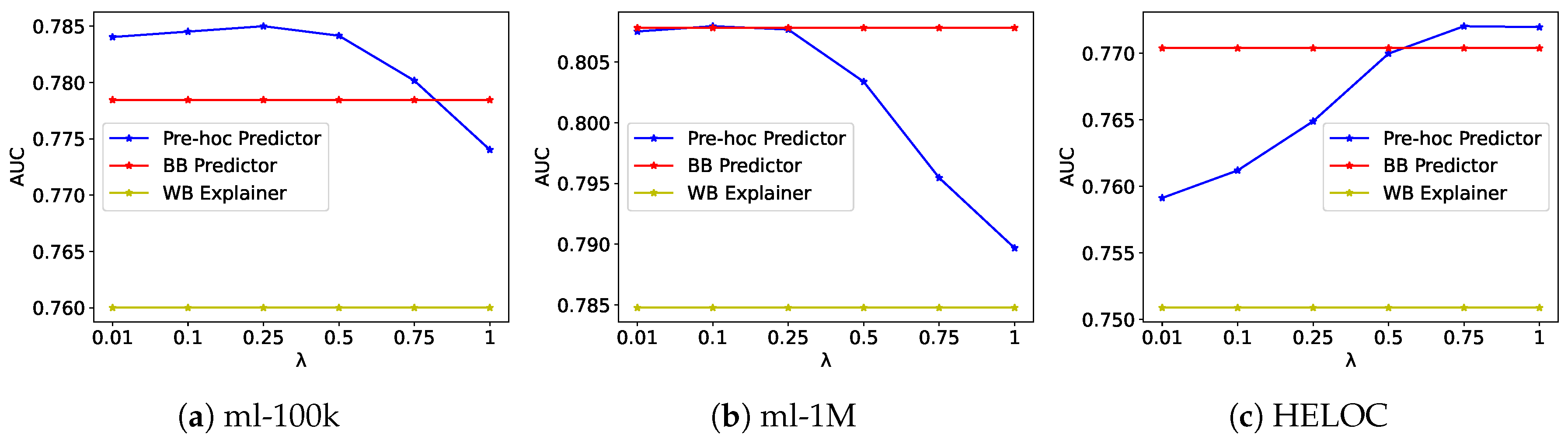
Figure 2.
Effect of explainability regularization parameter on accuracy and fidelity for Co-hoc Explainability Framework on the ml-100k (a), ml-1M (b), HELOC (c) datasets. Co-hoc Predictor is our proposed model, BB is the original black-box predictor model, and WB is the explainer model.
Figure 2.
Effect of explainability regularization parameter on accuracy and fidelity for Co-hoc Explainability Framework on the ml-100k (a), ml-1M (b), HELOC (c) datasets. Co-hoc Predictor is our proposed model, BB is the original black-box predictor model, and WB is the explainer model.
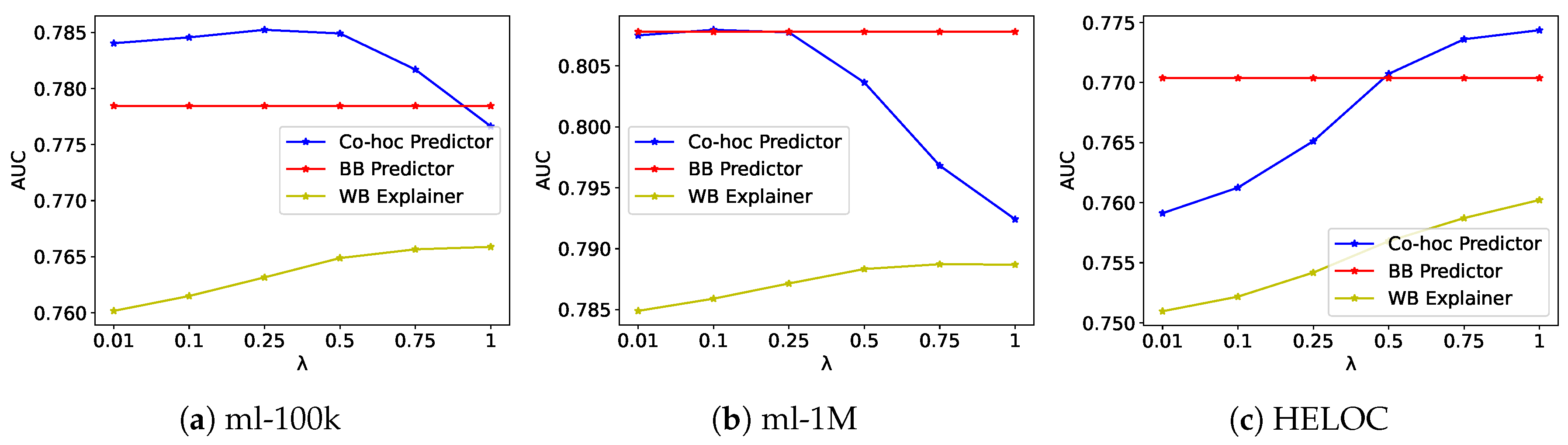
Figure 3.
Effect of explainability regularization parameter on point fidelity, neighborhood fidelity, and stability for the pre-hoc framework on the ML-100k Dataset results. Comparison of the Pre-hoc Framework with , for .
Figure 3.
Effect of explainability regularization parameter on point fidelity, neighborhood fidelity, and stability for the pre-hoc framework on the ML-100k Dataset results. Comparison of the Pre-hoc Framework with , for .
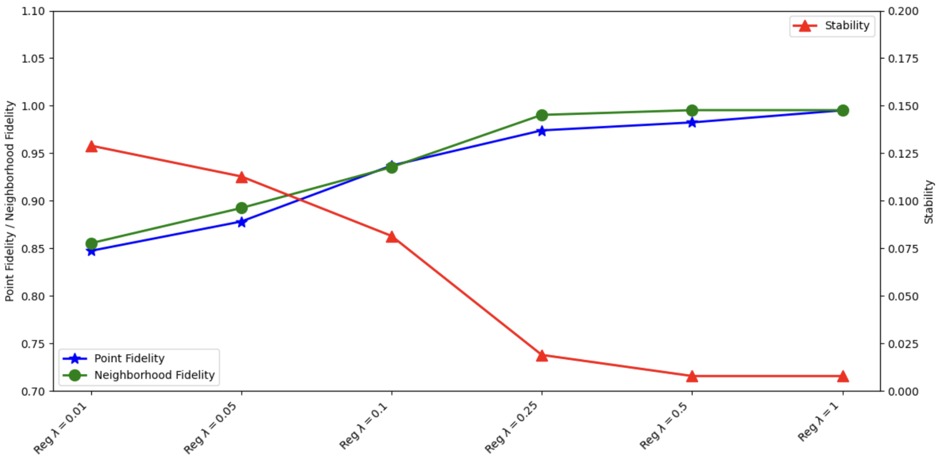
Figure 4.
HELOC Dataset: Top 10 Feature Importance scores from the global explanation of the pre-hoc framework.
Figure 4.
HELOC Dataset: Top 10 Feature Importance scores from the global explanation of the pre-hoc framework.
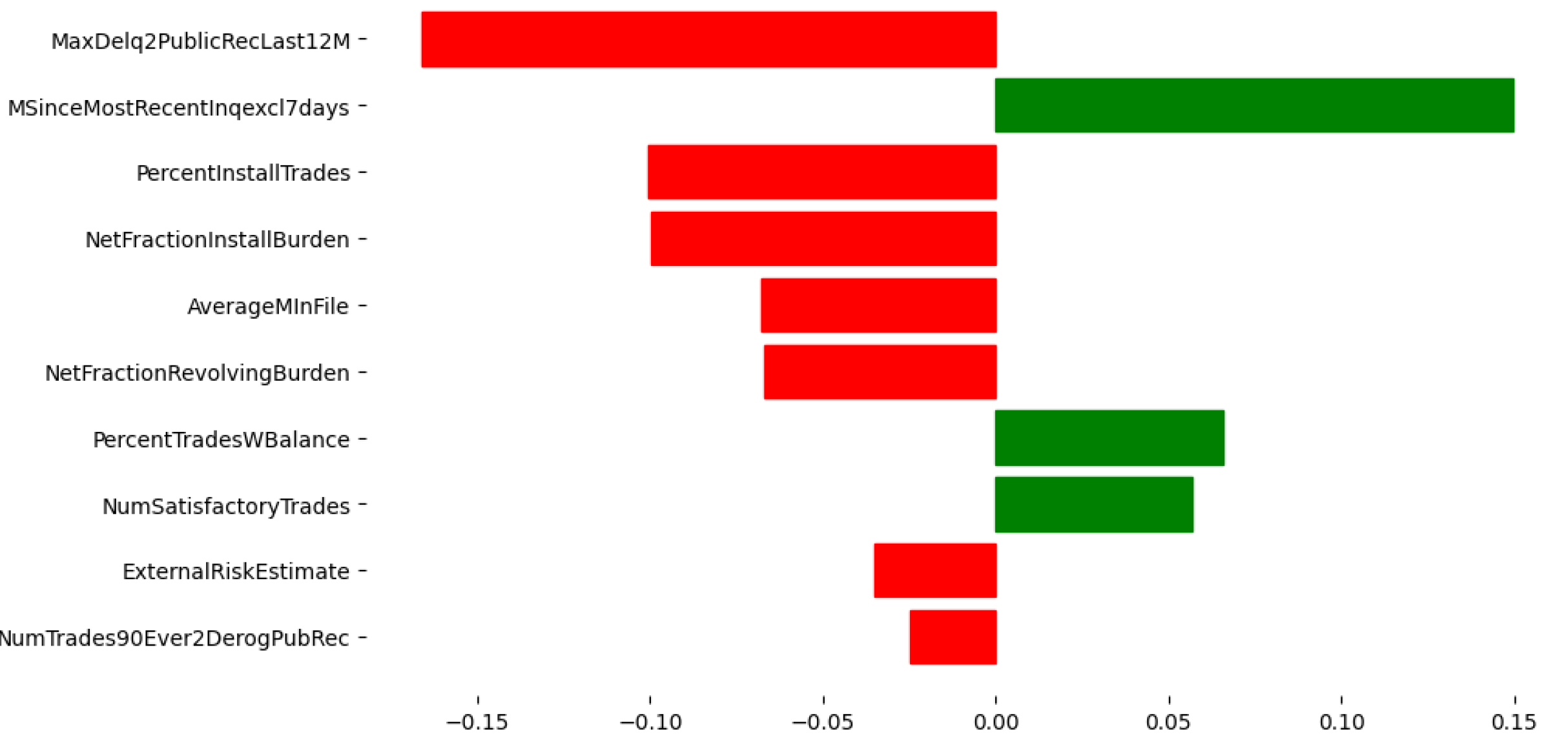
Figure 5.
HELOC Dataset: Local explanation for a Test Instance, showing the top 10 feature importance scores.
Figure 5.
HELOC Dataset: Local explanation for a Test Instance, showing the top 10 feature importance scores.
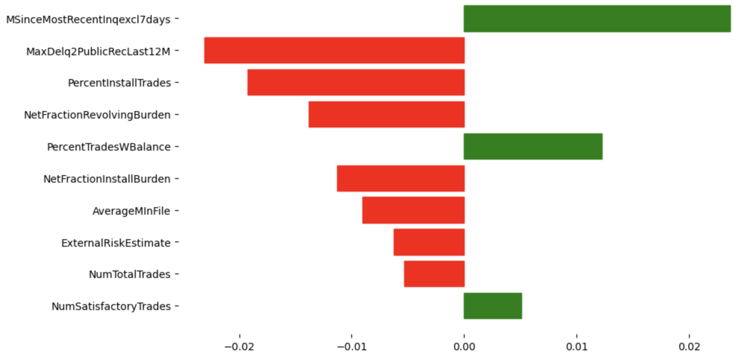

Table 1.
Model comparison in terms of prediction accuracy and fidelity on three real-world datasets. All metrics are computed with respective regularization parameters selected via validation. The best results are in bold.
Table 1.
Model comparison in terms of prediction accuracy and fidelity on three real-world datasets. All metrics are computed with respective regularization parameters selected via validation. The best results are in bold.
| Model | ML-100k | ML-1M | HELOC | |||
|---|---|---|---|---|---|---|
| AUC | Fidelity | AUC | Fidelity | AUC | Fidelity | |
| Explainer (WB) | 0.7655 | - | 0.7882 | - | 0.7616 | - |
| Original (BB) | 0.7784 | 0.8287 | 0.8078 | 0.8875 | 0.7703 | 0.7728 |
| Pre-hoc (BB) | 0.7801 | 0.9094 | 0.8033 | 0.9404 | 0.7698 | 0.8454 |
| Co-hoc (BB) | 0.7816 | 0.9194 | 0.8036 | 0.9484 | 0.7743 | 0.8572 |
Table 2.
HELOC Dataset: Comparison with LIME based on neighborhood fidelity and stability results (, ).
Table 2.
HELOC Dataset: Comparison with LIME based on neighborhood fidelity and stability results (, ).
| Explanation Method | Point Fidelity ↑ | Neighborhood Fidelity ↑ | Stability ↓ |
|---|---|---|---|
| LIME | 0.6083 ± 0.0050 | 0.6600 ± 0.1939 | 0.2152 ± 0.0175 |
| Pre-hoc Framework | 0.8270 ± 0.0260 | 0.9587 ± 0.0766 | 0.0623 ± 0.0110 |
| Co-hoc Framework | 0.8300 ± 0.0240 | 0.9647 ± 0.0575 | 0.0502 ± 0.0087 |
Table 3.
Effect of explainability regularization parameter on stability and fidelity for the pre-hoc framework on the ML-100k dataset. Comparison of the Pre-hoc Framework with , for in point fidelity, neighborhood fidelity, and stability results. "Reg" means that regularization was used.
Table 3.
Effect of explainability regularization parameter on stability and fidelity for the pre-hoc framework on the ML-100k dataset. Comparison of the Pre-hoc Framework with , for in point fidelity, neighborhood fidelity, and stability results. "Reg" means that regularization was used.
| Explanation Method | Point Fidelity ↑ | Neighborhood Fidelity ↑ | Stability ↓ |
|---|---|---|---|
| No-regularization | 0.8183 ± 0.3524 | 0.8050 ± 0.1268 | 0.3524 ± 0.0175 |
| Reg | 0.8473 ± 0.0351 | 0.8553 ± 0.1158 | 0.1290 ± 0.0010 |
| Reg | 0.8781 ± 0.0195 | 0.8923 ± 0.1043 | 0.1128 ± 0.0009 |
| Reg | 0.9370 ± 0.0230 | 0.9353 ± 0.0737 | 0.0815 ± 0.0019 |
| Reg | 0.9740 ± 0.0237 | 0.9903 ± 0.0329 | 0.0189 ± 0.0041 |
| Reg | 0.9824 ± 0.0234 | 0.9953 ± 0.0215 | 0.0078 ± 0.0010 |
| Reg | 0.9951 ± 0.0117 | 0.9953 ± 0.0215 | 0.0078 ± 0.0010 |
Table 4.
HELOC Dataset: Effect of neighborhood size on neighborhood fidelity, stability, and computation time for the pre-hoc framework ().
Table 4.
HELOC Dataset: Effect of neighborhood size on neighborhood fidelity, stability, and computation time for the pre-hoc framework ().
| Neighborhood Size | Neighborhood Fidelity ↑ | Stability ↓ | Computation Time (s) |
|---|---|---|---|
| 0.8833 ± 0.1939 | 0.2152 ± 0.0175 | 0.0121 ± 0.0014 | |
| 0.9350 ± 0.0381 | 0.0505 ± 0.0098 | 0.0127 ± 0.0009 | |
| 0.9670 ± 0.0013 | 0.0015 ± 0.00006 | 0.0144 ± 0.0061 |
Table 5.
HELOC Dataset: Computation time comparison for generating explanations on 100 test instances.
Table 5.
HELOC Dataset: Computation time comparison for generating explanations on 100 test instances.
| Method | Additional Training | Avg Explanation | Total Time for | Total Time for |
|---|---|---|---|---|
| Time (s) | Time (s) | Single Instance (s) | 100 Instances (s) | |
| LIME | - | 0.3812 ± 0.0828 | 0.3812 ± 0.0828 | 38.12 |
| Pre-hoc | 5.1020 ± 0.0315 | 0.0110 ± 0.0015 | 0.0110 ± 0.0015 | 6.20 |
| Co-hoc | 5.3960 ± 0.0330 | 0.0135 ± 0.0030 | 0.0135 ± 0.0030 | 6.75 |
Disclaimer/Publisher’s Note: The statements, opinions and data contained in all publications are solely those of the individual author(s) and contributor(s) and not of MDPI and/or the editor(s). MDPI and/or the editor(s) disclaim responsibility for any injury to people or property resulting from any ideas, methods, instructions or products referred to in the content. |
© 2025 by the authors. Licensee MDPI, Basel, Switzerland. This article is an open access article distributed under the terms and conditions of the Creative Commons Attribution (CC BY) license (http://creativecommons.org/licenses/by/4.0/).
Copyright: This open access article is published under a Creative Commons CC BY 4.0 license, which permit the free download, distribution, and reuse, provided that the author and preprint are cited in any reuse.


