
Submitted:
03 May 2025
Posted:
06 May 2025
You are already at the latest version
Abstract
Flexible photovoltaic (PV) support structures are widely used due to their large span, high land-use efficiency, low construction cost, and short construction periods. However, they exhibit low stiffness, light weight, and low damping, making them wind-sensitive and prone to wind-induced vibrations. Evaluating their dynamic performance remains challenging due to two critical limitations: the lack of field-measured modal property and the absence of reliably validated finite element (FE) models. In this study, a field modal testing of flexible PV support structure was conducted, and high-order modal properties were identified from multi-sensor data. Subsequently, response surface model was constructed, and the optimal combination of metal frame mass, cable initial tension, and column modeling was obtained through particle swarm optimization (PSO), leading to an updated FE model. The results show that the damping ratios of the first and second torsional modes is only 0.7% and 0.4%, respectively, highlighting the need to consider low damping properties. Besides, the deviation between the design and actual values of structural parameters cannot be ignored.
Keywords:
Flexible photovoltaic support structure
; Modal identification
; Field modal testing
; Finite element model updating
; Response surface
1. Introduction
In order to address the challenges of climate change and accommodate rapidly growing demand of energy, solar energy, being a clean and safe renewable energy source, has been widely adopted for power generation in recent years [1]. However, with the rapid expansion in solar power plants, flatten terrain resources are becoming increasingly scarce. As a result, flexible photovoltaic (PV) support systems have attracted significant interest due to their ability to adapt to complex environments such as deserts, mountains, fishponds, and sewage treatment plants. Despite these advantages, the inherent low stiffness and low damping ratios of cable-supported systems make them highly susceptible to wind-induced vibrations, which can further lead to PV modules being lifted, collisions, latent cracks, and even damage to the supporting structures. Therefore, wind-induced vibration must be taken into account during the design process. Current research methodologies for this issue primarily include wind tunnel aeroelastic tests as well as finite element (FE) simulations. However, the former lacks field-measured damping ratios for model calibration, while the latter suffers from insufficient validation against field-measured modal frequencies and mode shapes. Moreover, both methods seldom consider the changes in structural parameters of flexible PV supports during their service life. To address these limitations, field modal testing should be conducted to obtain accurate modal properties of flexible PV support structures. Meanwhile, FE model updating utilizing field-measured data is essential to develop a high-fidelity FE model that faithfully represents the actual structure.
Previous studies of flexible PV support structures based on wind tunnel aeroelastic tests have revealed that critical wind speeds are low and cables may suddenly collapse due to intensive vibration [2,3,4,5,6]. Furthermore, He et al. [7] observed flexible PV support fluttering in the aeroelastic tunnel testing, which was mainly characterized by coupled torsional and vertical motions. These findings underscore the high susceptibility of flexible PV support structures to flutter instability. The damping of flexible PV support structure is crucial in determining whether its vibration will diverge and lead to flutter. However, there is a notable lack of field studies providing accurate identification. Bao et al. [8] measured the first three order modal parameters of a solar tracker, but the modal properties of solar trackers notably differ from those of flexible PV supports. Lei et al. [9] conducted field testing on large-span flexible PV supports, obtaining only the vertical bending modal damping ratio and frequency. Therefore, more comprehensive field modal testing of flexible PV support structures is necessary to obtain other high-order modal properties.
In field modal testing, it is difficult to obtain the full-frequency response information of a structure using single type sensor. In 1973, the U.S. Department of Defense [10] first proposed data fusion from different types of sensors to obtain more accurate response estimates and improve system redundancy. Subsequently, this technology has been widely applied in the structural health monitoring of bridges, high-rise buildings, and transmission towers. In 2007, Smyth and Wu [11] proposed a multi-rate Kalman filter for the data fusion to address the issue of different sensor sampling rates. Based on the fusion of high-frequency accelerometer signals and low-frequency GNSS signals, Yang et al. [12] identified the modal frequencies of the Shanghai Tower; Moschas and Stiros [13] identified the modal frequencies and dynamic responses of a 40 m pedestrian steel bridge; Luo et al. [14] identified the high-order modes and more accurate modal parameters of a 660 m long suspension bridge. By fusing high-frequency accelerometer signals with low-frequency strain signals, Zhu et al. [15] obtained displacement responses of the Canton Tower covering both ultra-low and high frequencies; Zhang et al. [16] identified the modal frequencies and mode shapes of a 50 m high transmission tower. In recent years, with the development of optical sensors and computer vision technology, computer vision-based displacement measurement has been widely used due to its advantages of simple installation and low cost. However, image resolution, lighting conditions, and shooting distance can affect the accuracy of vision-based measurements [17]. Accelerometers, on the other hand, can capture high-frequency, small-amplitude vibrations, supplementing the limitations of vision-based methods. Therefore, Park et al. [18] proposed fusion of vision-based displacement with acceleration via a complementary filter and time synchronization algorithm to obtain displacement signals with reduced noise. Based on the fusion of high-frequency accelerometer signals and low-frequency vision-based displacement signals, Ma et al. [19] acquired high-frequency displacement signals at a single measurement point of a steel box girder pedestrian bridge in Korea; Xiu et al. [20] identified modal properties of a reinforced concrete frame structure. These studies indicate that current applications of multi-sensor data fusion mainly focus on bridges, high-rise buildings, and transmission towers, while there is a lack of research on new structural types such as PV supports. This gap highlights the need for further development of multi-sensor data fusion techniques tailored to the unique challenges of PV support structures.
While field modal testing provides the foundation for understanding the dynamic behavior of flexible PV supports, the absence of a unified FE modeling approach has led to significant discrepancies in wind vibration coefficients across existing studies. Xu et al. [21] recommended a theoretical value of 1.73 for the wind vibration coefficient. Du et al. [22] used ANSYS for FE analysis and reported wind vibration coefficients of 2.11 and 1.98 for the along-wind and vertical displacements of flexible PV support structures, respectively. Song et al. [23] conducted wind pressure time-history simulations and FE analysis, suggesting that the wind vibration coefficient for single-layer flexible PV support structures should be in the range of 1.3 to 1.7. Wang et al. [24,25,26] simulated fluctuating wind speeds using an autoregressive model and established multi-span FE models of flexible PV supports in SAP2000, comparing the dynamic response characteristics under different wind load. Among the above studies using FE analysis, Du et al. [22] and Song et al. [23] only established single-span models without considering support columns, treating the cable ends as fixed constraints. In contrast, Xu, Song and Wang et al [21,23,24,25,26] considered support columns in their modeling and developed multi-span models. It can be seen that there is currently no unified approach to modeling flexible PV support structures, which further leads to significant differences in the wind vibration coefficients calculated among the aforementioned studies [22,23,24,25,26]. Therefore, it is significant to conduct the FE model updating based on field measurement of flexible PV support structures.
In FE model updating, the direct method [27,28] adjusts the model by modifying the system’s stiffness, mass, and damping matrices. This method requires no iterative computation and always yields a convergent solution; however, the updated system matrices often lose their physical meaning, and nodal continuity cannot be ensured [29]. Moreover, the direct modification approach operates directly on the system matrices, it typically requires complete experimental modal data at multiple measurement points. To address these limitations, Mottershead and Friswell [30] proposed a sensitivity-based updating method, which adjusts material properties, geometric parameters, and boundary conditions of the model in accordance with measured responses. However, traditional sensitivity-based model updating methods require repeated calls to FE software, which is computationally inefficient. Furthermore, ill-conditioned sensitivity matrices may result in convergence difficulties [31]. To overcome these shortcomings, Guo and Zhang [32] introduced the response surface model, which utilizes explicit surrogate functions to approximate the implicit relationships in FE models, thus avoiding repeated FE computations and enabling more efficient convergence. Based on ambient vibration data from a six-span continuous beam bridge, Ren et al. [33] performed response surface-based FE model updating and compared the results with traditional sensitivity-based methods. The findings indicated that the response surface-based approach significantly improved updating efficiency and convergence speed. Fang [34] applied the response surface method to FE model updating and damage identification for the I-40 bridge; the results demonstrated that second-order polynomial and first-order linear models are capable of characterizing the relationship between structural parameters and responses. Although FE model updating has been widely applied in bridges and high-rise buildings, studies on its application to flexible PV support structures remain limited.
The remainder of this paper is organized as follows. Section 2 provides a detailed explanation of modal property identification based on multi-sensor data fusion, and the response surface-based FE model updating method for flexible PV support structures. Section 3 introduces the flexible PV support’s structure composition and the field modal testing scheme. Section 4 presents the field-measured high-order modal frequencies, damping ratios and spatial mode shapes of the flexible PV support, and fits the response surface to obtain the updated FE model. Section 5 concludes with a summary of the key findings.
2. Methodology
The flowchart of modal property identification and FE model updating for flexible PV support structures is shown in Figure 1. First, field modal testing of the flexible PV support structure is carried out. Subsequently, the VMD-SH method proposed by Cai et.al. [35] is employed to identify the modal frequencies and damping ratios. In the VMD-SH method, multi-sensor signals are first decomposed into a series of single-mode components using the variational mode decomposition (VMD) [36] method. The natural excitation technique (NExT) [37] is then used to convert these single-mode components into free decay signals. The smoothed discrete energy separation algorithm (SDESA) [38] is applied to the free decay signals to identify time-varying modal frequencies, while the half-cycle energy operator (HCEO) [39] is used to identify time-varying modal damping ratios. The modal shapes are identified from multi-sensor signals using a VMD-based approach. For FE model updating, response surface model for modal frequencies is first constructed. Then, the particle swarm optimization (PSO) [40] algorithm is employed on the response surface to search for the combination of modeling parameters that minimizes the error between the FE modal frequencies and the field-measured modal frequencies, thereby obtaining the updated FE model.
2.1. Identification of Modal Frequencies and Damping Ratios
VMD [36] is adopted as the primary signal decomposition technique owing to its capability to separate mixed signals into mutually independent components (MICs). In contrast to traditional approaches—which are often affected by problems such as mode mixing and end effects—VMD iteratively minimizes the bandwidth of each modal component while simultaneously determining its center frequency. The decomposition process is formulated as a constrained variational optimization problem, expressed as follows:
where represents each mode, is the center frequency, is the Dirac distribution, and is the input signal.
After decomposition, each single-mode component is processed using NExT [37] to obtain the free decay response. Subsequently, the SDESA [38] method is employed to identify the modal frequency as follows:
where is the discrete signal, is the sampling frequency and devotes the actual frequency of . This approach mitigates end effects, ensuring precise identification of natural frequencies.
To identify damping ratios, the HCEO [39] is applied to the free decay signals of each mode. This approach calculates the energy dissipated per vibration cycle and derives the damping ratio as follows:
where is the energy of each half-cycle.
While the original VMD-SH [35] was designed for frequency and damping ratio identification, this study proposes an extended approach to also identify mode shapes, as detailed in Section 3.2.
2.2. Identification of Mode Shapes
To obtain the mode shape of a specific mode, it is necessary to consider the single-mode responses of the structure at all sensor locations. The modal vector is constructed from the single-mode response values at all sensor positions at an identical time instant tm, which is typically selected at a local minimum or maximum. Accordingly, the modal vector of the k-th mode for the structure can be expressed as [41]:
where represents the modal response of the k-th mode at the j-th senser location, is the time instant when a local minimum or maximum of the modal response occurs, and N is the total number of sensors. Figure 2 illustrates the process of identifying the k-th mode shape using signals from three sensors.
The modal assurance criterion (MAC) [42] serves as a quantitative measure of the consistency (or degree of linear correlation) between estimates of a modal vector. The MAC enables the comparison of modal vectors obtained from different sources, thereby allowing for an assessment of the consistency between FE analysis results and field-measured results. The MAC is defined as follows [42]:
In this equation, is modal vector for reference c mode r, is modal vector for reference d mode r. MAC is between 0 and 1, with 0 representing no consistent correspondence and 1 representing consistent correspondence.
2.3. Response Surface-Based FE Model Updating Methodology
The overall procedure of response surface-based FE model updating is illustrated in Figure 3.
For flexible PV support structures, their large spans and low stiffness make them susceptible to wind-induced vibrations [43]. To ensure that the updated model more accurately represents the actual dynamic characteristics of the structure, the first four modal frequencies are selected as the response features for model updating.
The selection of updating parameters for flexible PV support structure models differs significantly from that for buildings and bridges. The main reasons are as follows: the components of the support are mostly standardized, with minimal differences in size and material properties between them; as a steel structure, the mechanical properties of the support are more stable compared to concrete, but it is also more susceptible to corrosion; the flexible support is a prestressed cable-supported structure, and under wind loads, slippage at the cable anchor points can lead to a decrease in cable tension; PV modules consist of aluminum frames, laminates, and junction boxes, and previous modeling of PV modules often assumed them to be uniformly distributed panels, which overlooks the mass non-uniformity of the aluminum frames and laminate layers. Based on these considerations, the preliminary selection of updating parameters includes the mass of the metal frame M, cable initial tension T and support column modeling L.
When a complex or unknown relationship exists between the modal frequency y of a flexible PV support structure and its physical parameters, this relationship can be represented by an explicit hypersurface function, that is, a response surface model [33]:
Where,, denotes the statistical error, is an unknown implicit function. Since is unknow, researchers aim to estimate using an approximate but explicit function, which can be achieved by the response surface model . The estimated response can be expressed as:
Where, represents the error of the response surface, which should be minimized as much as possible. Subsequently, the response surface can be used to substitute for the physical model in numerical analysis.
The selection of the response surface function type first requires that its mathematical expression can adequately describe the true relationship between the input parameters and the output response. Second, the expression should contain the minimum number of terms to reduce the required number of sampling points and enhance interpretability. For most engineering problems, a standard quadratic polynomial function can be used to represent the physical system [33]:
Where, denotes the response feature, specifically the first four modal frequencies of the flexible PV support structure, with each frequency corresponding to a separate response surface model. represents the range of values for the updating parameters, and , , , are the regression coefficients.
Equation (8) can be represented in matrix form as:
Where is the response vector, B is the matrix of regression coefficients, and e contains all errors.
The unbiased estimate b of the regression coefficient matrix B can be obtained by the least square method:
Finally, the response estimated by the response surface can be expressed as:
To ensure its reliability for future applications, response surface model must be validated. This validation process involves two key aspects: assessing the model’s fitting performance on design points and evaluating its predictive capability with unseen data. Several indices are used for this validation:
represents the interpretability of the model, with a range of [0,1]. A value close to 1 indicates a high level of fit. A smaller RMSE indicates a smaller model error.
The optimization problem in FE model updating can be expressed as minimizing the error between the field-measured results and the FE analysis results:
Where, PFEM and PEXP represent the external excitations applied to the FE modal and the actual structure, respectively. and denote certain mappings of the FE model and the actual structure. represents the error function, and the feasible domain of the updating parameters X is [XL, XU]. FE model updating requires minimizing the error function.
In this study, the first four modal frequencies are chosen as the response features, . Each response feature is fitted with an independent response surface function . So, Equation (14) can be rewritten as:
Equation (15) represents a multi-objective optimization problem, which can be transformed into a single-objective optimization problem:
The single-objective optimization problem under the constraint of Equation (16) is subsequently solved using PSO [40]. In PSO, particles are randomly initialized in a D-dimensional parameter space. Each particle has two attributes: a velocity , representing the direction and magnitude of iteration, and a position , representing a combination of updating parameters. The velocity and position are updated as follows:
Where, denotes the iteration number; is the local best position of particle in dimension , and is the global best position of the swarm in dimension ; and are random numbers in the interval [0,1]; is the inertia weight; and are the local and global learning coefficients, respectively. Therefore, the update direction of each particle incorporates the local best direction, the global best direction, and the inertial direction.
3. Field Modal Testing for PV Support Structure
3.1. PV Support Structure
The flexible PV support structure consisted of concrete foundations, support columns, diagonal cables, support cables, and the PV modules fixed to the support cables through metal clamp fixing, as shown in Figure 4(a). The structure tested in this study is shown in Figure 4(b). Each PV module measures 2172 mm × 1303 mm × 35 mm with a 26 mm inter-module spacing at a tilt angle of 15°. The span between the columns is 21.9 m. Two support-cables, each with a diameter of 16 mm and an initial tension of 60 kN, connected the ends of the span. 16 PV modules were mounted on the support cable secured by metal clamp fixings. The support columns, made of Q345 steel, stood 3.5 meters high, and were fixed to concrete foundations. The diagonal cables were anchored to the concrete foundations and connected to the top of the support columns. This configuration balanced the initial tension of the support-cables and ensure the columns remain stable.
The FE model was established using ANSYS APDL software as shown in Figure 5. The cable is modeled using LINK180 with an initial tension of 60 kN applied. The cable has a Young's modulus of 1.95×10¹¹ Pa, a density of 7850 kg/m3 and a Poisson's ratio of 0.3. The PV module was modeled using SHELL181, with a Young's modulus of 7.2×10⁹ Pa, a density of 304.25 kg/m3, and a Poisson's ratio of 0.33. The steel support columns were modeled by the BEAM188 element. The bottoms of the columns were constrained in all degrees of freedom in the FE model. The columns have a Young's modulus of 2.06×10¹¹Pa, a density of 7850 kg/m3 and a Poisson's ratio of 0.3.
Figure 6 presents the first four mode shapes obtained from the FE model. The first-order mode is the half-wave vertical bending mode with the maximum displacement occurring at the mid-span. The second-order mode is the first-order torsional mode with maximum displacements occurring at the front and rear ends of the mid-span PV panels. The third-order mode is the full wave vertical bending mode with the maximum displacement occurring at the quarter-span PV panels. The fourth-order mode is the second-order torsional mode with maximum displacements occurring at the front and rear ends of the quarter-span PV panels. And the first four orders of modal frequencies derived from FE analysis are 1.69 Hz, 2.20 Hz, 3.08 Hz and 4.24 Hz, respectively.
3.2. Field Modal Testing Scheme
Field modal testing integrates two complementary measurement modalities: (1)A vision-based measurement system employing camera sampling at 30 frames per second, with paper markers positioned on PV modules as measurement targets, as shown in Figure 7(a). (2) Velocity sensors with frequency range from 1Hz to 100 Hz sampled at 50 Hz, as shown in Figure 7(b).
For the first-order mode, the camera and paper markers are arranged as shown in Figure 8(a). The three measurement points were clustered in a centralized area, which did not fully capture the overall structural behavior—primarily due to limitations in camera placement. The flexible PV structure is situated on a hillside, where the sloped terrain and the short spacing between rows of PV supports constrain the available space for camera positioning. For the second-order mode, the camera and paper markers are arranged as shown in Figure 8(b). In this case, the markers were distributed both along the spanwise and vertical directions to more effectively capture the spatial characteristics of the mode shape. For the third- and fourth-order modal tests, velocity sensors were employed due to the low and weak vibration energy associated with these modes, which requires sensors with higher resolution to accurately record the signals, whether the excitations are artificial or ambient. The velocity sensor arrangement for the third- and fourth-order modal testing is shown in Figure 8(c).
The optimal location for excitation was determined based on the FE modal analysis results, with the theoretical ideal position corresponding to the maximum response in the mode shape profile. During the field testing, it was observed that the second-order torsional mode was difficult to excite using artificial means. Therefore, ambient wind excitation was utilized as a supplementary approach to facilitate the activation of this mode.
The test conditions are summarized in Table 1.
3.3. Data from Field Modal Testing
Computer vision-based measurement was used in test 1 and 2. The vibration displacement signals at the measurement points were identified from videos captured by monocular camera. The camera view for test 1 is shown in Figure 9(a), where three artificial markers and their corresponding measurement point numbers are indicated. The camera view for test 2 is shown in Figure 9(b), where eight artificial markers and measurement point numbers are labeled.
The free decay segment of the signal from test 1 and 2 was extracted, as shown in Figure 10(a) and Figure 10(b). The amplitude ratios among measurement points remain stable, and the power spectra all exhibited a single peak, which is close to the frequency from the FE modal analysis results. Therefore, it can be concluded that test 1 and 2 effectively and independently excited target mode.
In test 3, velocity sensors were used, and the free decay segment was extracted. The velocity signals and corresponding power spectra are shown in Figure 10(c). Although the target mode is the full-wave vertical bending, the power spectrum indicates that the vibration was dominated by the half-wave vertical bending mode. The full-wave vertical bending mode exhibited low vibration energy and was difficult to excite independently. The modal frequency of the full-wave vertical bending mode was 2.98 Hz, which is close to the FE modal analysis result of 3.04 Hz.
In test 4, velocity sensors were used, and 50 minutes of vibration signal under ambient excitation were selected. The time history and power spectra are shown in Figure 10(d). The ambient excitation effectively excited the second-order torsional mode, with the modal frequency of 3.53 Hz.
4. Results and Analysis
4.1. Modal Frequency and Damping Ratio Identification
The measured data from velocity sensor 1 in test 4 was analyzed. The time history of the signal and the concerned frequency spectrum are presented in Figure 11. In the VMD algorithm, parameter was set to 10 to allow for consideration of more vibration modes and removing low and high frequency vibrations that are not structural vibration. Additionally, the convergence parameter was set to a value of 10-8. Performing the VMD on the pure vibration signals after low-pass filter with a cutoff frequency of 5 Hz, MICs and corresponding spectrum are shown in Figure 12. The spectrum values for the four main frequencies of MICs are 2931, 8644, 1820, and 6633, as depicted in Figure 12, which are remarkably close to the values presented in Fig. 11 (3053, 8639, 1845, and 6707), indicating that there is almost no energy leakage.
By applying the NExT method to each MICs, the free decay signals are obtained. Subsequently, the SDESA and HT methods are used to extract the amplitude envelope and time-varying frequency. The identified frequencies () and damping ratios () are listed in Table 2.
4.2. Mode Shape Identification
Taking the second-order torsional mode as an example, test 4 is selected for analysis. The power spectra show multiple peaks and is dominated by first- and second-order modes as shown in Figure 10(d). In the VMD method, parameter K was set to 10 to consider more modes, and the convergence parameter ε was set to 10-7. Performing the VMD, the decomposed second-order torsional modal response and corresponding spectra are shown in Figure 13(a), where the Fourier spectra reveal a 3.53 Hz single peak, effectively separating the target modal response from the others. The acceleration signal is used in Figure 13(a) to amplify the second-order torsional modal components and reduce the energy proportion of the first- and second-order modal components, allowing the VMD method to better retain the second-order torsional modal response component.
According to Equation (4), the modal vector from point 1 to 4 was obtained to reconstruct the second-order torsional mode shape, as shown in Figure 13 (b). The modal vectors and corresponding MAC value are given in Table 3.
The test cases 1 to 3 are selected, and the first to third mode shapes are identified in the same way. The results are presented in Figure 14 to Figure 16. The modal vectors and corresponding MAC values are given in Table 3. Overall, the MAC values for the first four mode shapes are close to one, indicating a high degree of agreement between the field testing results and the FE model in terms of mode shapes, thereby validating the accuracy of the mode shape identification method.
4.3. Response Surface Model
The first four modal frequencies of the flexible PV support structure are selected as the response features. The corresponding frequencies obtained from the FE model and field-measured results are presented in Table 4.
The updating parameters are the mass of the metal frame , cable initial tension , and column modeling . In the initial FE model, the cable initial tension is 60 kN, the PV modules do not consider the mass of the metal frame, and the columns are not modeled. Currently, there is no reference for selecting the upper and lower bounds of the updating parameters for flexible photovoltaic supports. However, during the use of the structure, the tension in the cables may decrease due to wind-induced vibration effects, so the upper bound for cable initial tension is set to 60 kN, and the lower bound is set to 0.6×60kN. The mass of the metal frame is an additional factor, with the lower bound set to 0 kg and the upper bound set to 4 kg. Column modeling has only two values, modeled or not modeled, set to 0 or 1. The range of updating parameters is shown in Table 5.
When considering the column modeling , all of the first four modal frequencies decrease, effectively improving the accuracy of the finite element model. Since the column modeling is a binary variable, taking values of only 0 and 1, it is concluded that column modeling should be considered, setting . Consequently, the updating parameters involved in the fitting process exclude , retaining only and .
The complete factorial design method is chosen to comprehensively analyze all effects. The mass of the metal frame is varied in intervals of 0.2 kg, generating 21 parameter values, while the cable initial tension is varied in intervals of 2% of , also generating 21 parameter values. Combining all parameter values results in a total of sample points.
The response surface fitting results are shown in Figure 17, and the response surface functions represented by quadratic polynomials are given in Equations (19) to (22).
According to Equations (12) and (13), the fitting validation results are shown in Table 6. The values are close to 1 and the RMSE values are small, indicating that the fitting model has high accuracy and can effectively represent the relationship between the updating parameters and and the response features .
4.4. Finite Element Model Updating
The optimization problem, as shown in Equation (16) was solved in the parameter space using the PSO algorithm. The PSO parameter settings were as follows: the population size was set to 50, the maximum number of iterations was 50, and both the global learning rate and the local learning rate were set to 1.49. After 41 iterations, the objective function converged to a stable minimum value of 0.03657. The updated parameters are summarized in Table 7, and the convergence curve of the objective function is presented in Figure 18.
The optimization results indicate that the cable initial tension in the updated model is 0.866 times the design value, and the metal frame mass is 2 kg. The possible reason is that the cable was not tensioned to the design value during construction, or a tension loss of 13.4% occurred during service. In addition, the mass of the metal frame should be accounted for in the modeling process, and its value is 2 kg.
By incorporating the updated and into the FE model, the first four modal frequencies were calculated, as shown in Table 8. Results indicates that the relative errors between the updated model and the measured results for the first, second, and fourth modal frequencies have significantly decreased, from 13.78%, 24.22%, and 20.31% to 0.47%, 1.52%, and 0.28%, respectively. However, the relative error for the third modal frequency in the updated model increased from 3.38% to 8.46%.

Table 2.
Summary of the test cases.
| Response feature | Field-measured | Initial value | Updated value | Initial error | Updated error |
|---|---|---|---|---|---|
| f1 (Hz) | 1.488 | 1.693 | 1.481 | 13.78% | 0.47% |
| f2 (Hz) | 1.775 | 2.205 | 1.802 | 24.22% | 1.52% |
| f3 (Hz) | 2.980 | 3.081 | 2.728 | 3.38% | 8.46% |
| f4 (Hz) | 3.526 | 4.242 | 3.516 | 20.31% | 0.28% |
5. Conclusions
This paper focuses on flexible PV support structures, conducting field modal testing and proposing a modal property identification method based on multi-source data fusion. The high-order modal properties of the actual flexible PV structures were obtained through field measurements. Based on the measured modal properties, response surface-based FE model updating of the flexible PV support structure was accomplished. The following conclusions can be drawn from the study:
(1) The effectiveness of the field modal testing method was verified. The results indicate that the computer vision-based measurement enables high-precision identification of the lower-order vibration modes of the PV support structure. For high-order modes, due to weaker vibration energy, it is necessary to comprehensively analyze the data from both the computer vision system and velocity sensors.
(2) The first four modal properties of the flexible PV support structure were identified. It is noteworthy that the damping ratios of the first- and second-order torsional modes are only 0.7% and 0.4%, respectively, indicating that the low-damping characteristics of the flexible PV structure should be given particular attention in the design practice.
(3) A response surface-based finite element model updating method for flexible PV support structures was proposed. The high fitting accuracy of the response surface surrogate model demonstrates its feasibility as an alternative to full finite element analyses. The updated finite element model shows its dynamic characteristics closely match to the actual structure.
Author Contributions
Conceptualization, C.Y. and M.H.; methodology, C.Y. and K.C.; formal analysis C.Y. and K.C.; investigation, M.H. and C.Y; data curation C.Y. and X.L.; writing—original draft preparation, C.Y.; writing—review and editing, all authors; supervision, M.H. All authors have read and agreed to the published version of the manuscript.
Funding
This research was partially supported by Ningbo Key R&D Program (Project No. 2023Z221 and 2024Z287), the National Natural Science Foundation of China (Project No. 52478564) and Research Grants Council of Hong Kong Theme-based Research Scheme (Grant No. T22-501/23-R).
Institutional Review Board Statement
Not applicable.
Informed Consent Statement
Not applicable.
Data Availability Statement
Not applicable.
Acknowledgments
The authors would like to acknowledge Jiangsu Evershine Energy Technology Co., Ltd. for providing organization and coordination assistance during the field testing.
Conflicts of Interest
The authors declare no conflicts of interest.
Abbreviations
The following abbreviations are used in this manuscript:
| PV | Photovoltaic |
| FE | Finite element |
| PSO | Particle swarm optimization |
| VMD | Variational mode decomposition |
| NExT | Natural excitation technique |
| SDESA | Smoothed discrete energy separation algorithm |
| HCEO | Half-cycle energy operator |
| MIC | Mutually independent component |
References
- Ding, H.; He, X.; Jing, H.; Wu, X.; Weng, X. Design Method of Primary Structures of a Cost-Effective Cable-Supported Photovoltaic System. Applied Sciences 2023, 13, 2968. [Google Scholar] [CrossRef]
- Tamura, Y.; Kim, Y.C.; Yoshida, A.; Itoh, T. Wind-Induced Vibration Experiment on Solar Wing. MATEC Web of Conferences 2015, 24, 04006. [Google Scholar] [CrossRef]
- Kim, Y.C.; Shan, W.; Yang, Q.S.; Tamura, Y.; Yoshida, A.; Ito, T. Effect of Panel Shapes on Wind-Induced Vibrations of Solar Wing System under Various Wind Environments. Journal of Structural Engineering. 2020, 146, 04020104. [Google Scholar] [CrossRef]
- Kim, Y.; Tamura, Y.; Yoshida, A.; Ito, T.; Shan, W.; Yang, Q. Experimental Investigation of Aerodynamic Vibrations of Solar Wing System. Advances in Structural Engineering 2018, 21, 2217–2226. [Google Scholar] [CrossRef]
- Liu, J.; Li, S.; Luo, J.; Chen, Z. Experimental Study on Critical Wind Velocity of a 33-Meter-Span Flexible Photovoltaic Support Structure and Its Mitigation. Journal of Wind Engineering and Industrial Aerodynamics 2023, 236, 105355. [Google Scholar] [CrossRef]
- Liu, J.; Li, S.; Chen, Z. Experimental Study on Effect Factors of Wind-Induced Response of Flexible Photovoltaic Support Structure. Ocean Engineering 2024, 307, 118199. [Google Scholar] [CrossRef]
- He, X.H.; Ding, H.; Jing, H.Q.; Zhang, F.; Wu, X.P.; Weng, X.J. Wind-Induced Vibration and Its Suppression of Photovoltaic Modules Supported by Suspension Cables. Journal of Wind Engineering and Industrial Aerodynamics 2020, 206, 104275. [Google Scholar] [CrossRef]
- Bao, T.; Li, Z.; Pu, O.; Chan, R.W.K.; Zhao, Z.; Pan, Y.; Yang, Y.; Huang, B.; Wu, H. Modal Analysis of Tracking Photovoltaic Support System. Solar Energy 2023, 265, 112088. [Google Scholar] [CrossRef]
- Lei, Z.H. Research on Wind-induced Vibration Characteristics and Control of Large-span Cable-supported Photovoltaic Support Brackets Structure by Experimental Test. Master, Central South University, China, 2023.
- White, F.E. Data fusion lexicon, joint directors of laboratories, technical panel for C3, data fusion sub-panel. San Diego, CA: Naval Ocean Systems Center, 1987.
- Smyth, A.; Wu, M. Multi-Rate Kalman Filtering for the Data Fusion of Displacement and Acceleration Response Measurements in Dynamic System Monitoring. Mechanical Systems and Signal Processing 2007, 21, 706–723. [Google Scholar] [CrossRef]
- Yang, M.; Wu, J.; Zhang, Q. GNSS and Accelerometer Data Fusion by Variational Bayesian Adaptive Multi-Rate Kalman Filtering for Dynamic Displacement Estimation of Super High-Rise Buildings. Engineering Structures 2025, 325, 119396. [Google Scholar] [CrossRef]
- Moschas, F.; Stiros, S. Measurement of the Dynamic Displacements and of the Modal Frequencies of a Short-Span Pedestrian Bridge Using GPS and an Accelerometer. Engineering Structures 2011, 33, 10–17. [Google Scholar] [CrossRef]
- Luo, L.; Liu, Z.; Liu, H. Operational Modal Analysis Method for Long-Span Suspension Bridges Based on Data Fusion. 2024 4th International Conference on Computer Science and Blockchain (CCSB). IEEE, 2024.
- Zhu, H.; Gao, K.; Xia, Y. Multi-rate data fusion for dynamic displacement measurement of beam-like supertall structures using acceleration and strain sensors. Structural Health Monitoring. 2019, 19(2), 520–536. [Google Scholar] [CrossRef]
- Zhang, Q.; Fu, X.; Ren, L.; Li, H.-N. Two-Dimensional Full-Field Displacement Reconstruction of Lattice Towers Using Data Fusion Method: Theoretical Study and Experimental Validation. Thin-Walled Structures 2023, 182, 110189. [Google Scholar] [CrossRef]
- Huang, M.; Li, X.; Cai, K.; Kareem, A. Motion Adaptive Vision-Based Vibration Measurement and Modal Identification for the Roof Masts of a Tall Building. Engineering Structures 2025, 323, 119278. [Google Scholar] [CrossRef]
- Park, J.W.; Moon, D.S.; Yoon, H.; Gomez, F.; Spencer, B.F., Jr.; Kim, J.R. Visual-Inertial Displacement Sensing Using Data Fusion of Vision-Based Displacement with Acceleration. Structural Control and Health Monitoring 2018, 25, e2122. [Google Scholar] [CrossRef]
- Ma, Z.; Choi, J.; Sohn, H. Real-time Structural Displacement Estimation by Fusing Asynchronous Acceleration and Computer Vision Measurements. Computer Aided Civil and Infrastructure Engineering 2022, 37, 688–703. [Google Scholar] [CrossRef]
- Xiu, C.; Weng, Y.; Shi, W. Vision and Vibration Data Fusion-Based Structural Dynamic Displacement Measurement with Test Validation. Sensors 2023, 23, 4547. [Google Scholar] [CrossRef] [PubMed]
- Xu, Z.; Hou, G.; Zhang, Z.; Wang, W.; Fan, H.; Shi, J. Numerical analysis of wind-induced vibration coefficient of fish-belt PV cable truss. Solar Energy 2019, 02, 46–49. (In Chinese) [Google Scholar]
- Du, H.; Xu, H.W.; Zhang, Y.L. Wind pressure characteristics and wind vibration response of long-span flexible photovoltaic support structure. Journal of Harbin Institute of Technology 2022, 54, 67–74. (In Chinese) [Google Scholar]
- Song, Y.M.; Yuan, H.X.; Du, X.X.; Wang, R.L. Research on static and dynamic response of single layer flexible photovoltaic support structure. Building Structure 2023, 1, 8. (In Chinese) [Google Scholar]
- Wang, Z.G.; Zhao, F.F.; Ji, C.M.; Peng, X.F.; Shen, T. Analysis of vibration control of multi-row large-span flexible photovoltaic supports. Engineering Journal of Wuhan University 2020, 53, 29–34. (In Chinese) [Google Scholar]
- Wang, Z.G.; Zhao, F.F.; Ji, C.M.; Peng, X.F.; Shen, T. Wind-induced vibration analysis of multi-row and multi-span flexible photovoltaic support. Engineering Journal of Wuhan University 2021, 2021, 75–79. (In Chinese) [Google Scholar]
- Wang, Z.G.; Zhao, F.F.; Ji, C.M.; Peng, X.F.; Shen, T. A comparative analysis of wind vibration response of large-span flexible photovoltaic support with stabilizing cable. Engineering Journal of Wuhan University 2022, 55, 33–38. (In Chinese) [Google Scholar]
- Smith, S.W.; Beattie, C.A. Secant-method adjustment for structural models. AIAA journal 1991, 29, 119–126. [Google Scholar] [CrossRef]
- Levin, R.I.; Waters, T.P.; Lieven, N.A. Required precision and valid methodologies for dynamic finite element model updating. Journal of Vibration and Acoustics 1998, 120, 733–741. [Google Scholar] [CrossRef]
- Friswell, M.I.; Mottershead, J.E. Finite Element Model Updating in Structural Dynamics; Springer: Berlin, Germany, 1995; Volume 3, pp. 45–78. [Google Scholar]
- Mottershead, J.E.; Friswell, M.I. Model updating in structural dynamics: a survey. Journal of sound and vibration 1993, 167(2), 347–375. [Google Scholar] [CrossRef]
- Link, M. Updating of analytical models—review of numerical procedures and application aspects. In Proc., Structural Dynamics Forum SD2000, Baldock, UK, April, 1999.
- Guo, Q.T.; Zhang, L.M. Finite element model updating based on response surface methodology. In Proceedings of the 22nd IMAC, Baldock, UK; 1999. [Google Scholar]
- Ren, W.X.; Fang, S.E.; Deng, M.Y. Response Surface–Based Finite-Element-Model Updating Using Structural Static Responses. Journal of Engineering Mechanics 2011, 137, 248–257. [Google Scholar] [CrossRef]
- Fang, S.E. Studies on Structural Damage Detection by Finite Element Model Updating. Doctor, Central South University, China, 2010.
- Cai, K.; Huang, M.; Li, X.; Xu, H.; Li, B.; Yang, C. Modal Parameter Identification of Tall Buildings Based on Variational Mode Decomposition and Energy Separation. Wind and Structures 2023, 37, 445–460. [Google Scholar] [CrossRef]
- Dragomiretskiy, K.; Zosso, D. Variational Mode Decomposition. IEEE Transactions on Signal Processing. 2014, 62, 531–544. [Google Scholar] [CrossRef]
- James, G.H. The natural excitation technique (NExT) for modal parameter extraction from operating structures. J Anal Exp Modal Anal 1995, 10(4), 260. [Google Scholar]
- Maragos, P.; Kaiser, J.F.; Quatieri, T.F. Energy Separation in Signal Modulations with Application to Speech Analysis. IEEE Transactions on Signal Processing 1993, 41, 3024–3051. [Google Scholar] [CrossRef]
- Huang, F.L.; Wang, X.M.; Chen, Z.Q.; He, X.H.; Ni, Y.Q. A New Approach to Identification of Structural Damping Ratios. Journal of Sound and Vibration 2007, 303, 144–153. [Google Scholar] [CrossRef]
- Kennedy, J.; Eberhart, R. Particle swarm optimization. In Proceedings of ICNN'95-international conference on neural networks, ieee, November, 1995.
- Bagheri, A.; Ozbulut, O.E.; Harris, D.K. Structural System Identification Based on Variational Mode Decomposition. Journal of Sound and Vibration 2018, 417, 182–197. [Google Scholar] [CrossRef]
- Allemang, R.J. The Modal Assurance Criterion – Twenty Years of Use and Abuse. Sound and Vibration 2003, 37(8), 14–23. [Google Scholar]
- Xu, H.; Ding, K.; Shen, G.; Du, H.; Chen, Y. Experimental Investigation on Wind-Induced Vibration of Photovoltaic Modules Supported by Suspension Cables. Engineering Structures 2024, 299, 117125. [Google Scholar] [CrossRef]
Figure 1.
Flowchart for modal property identification and FE model updating of flexible PV support structure.
Figure 1.
Flowchart for modal property identification and FE model updating of flexible PV support structure.
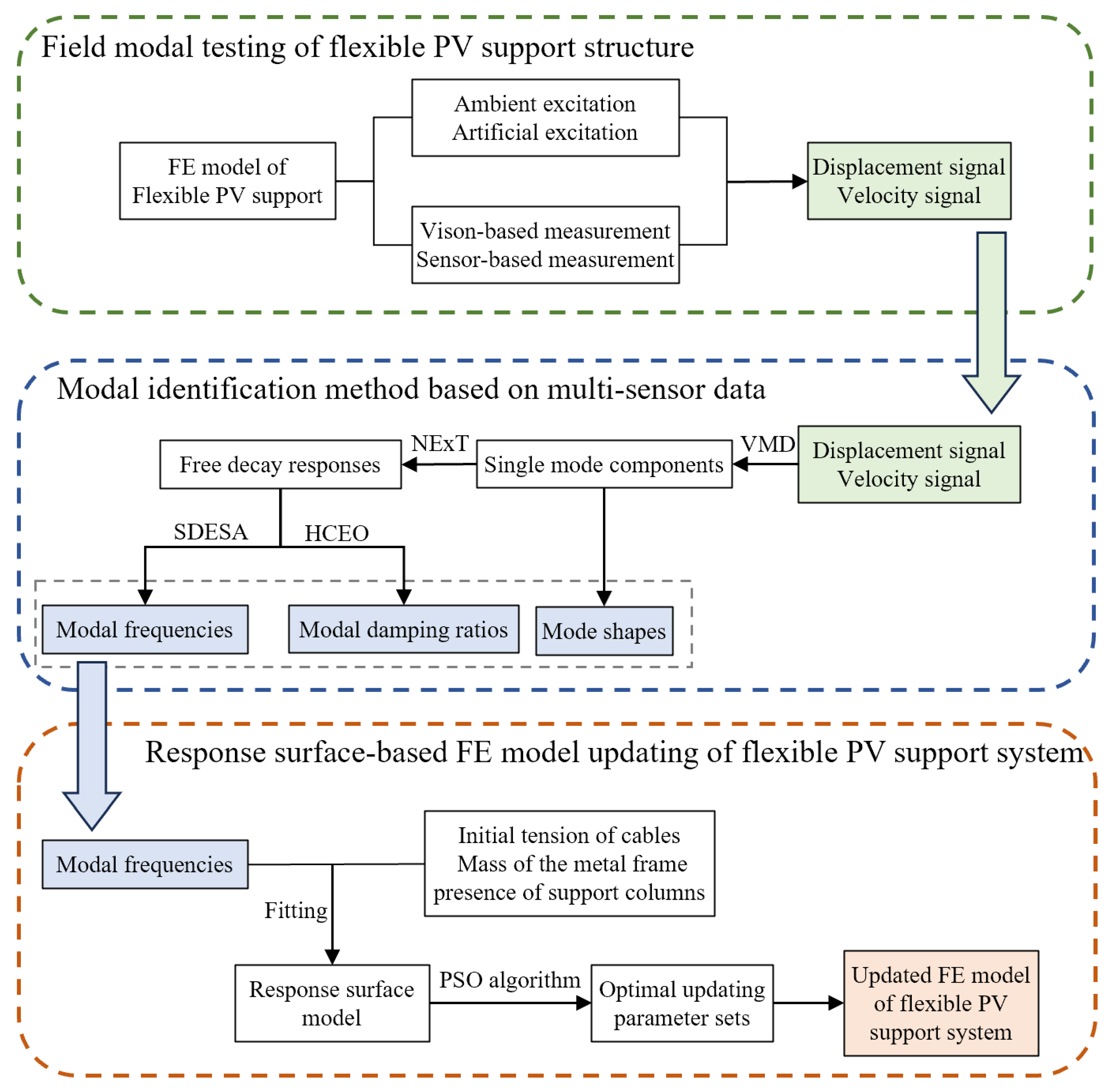
Figure 2.
Illustration of the mode shape identification from modal responses.
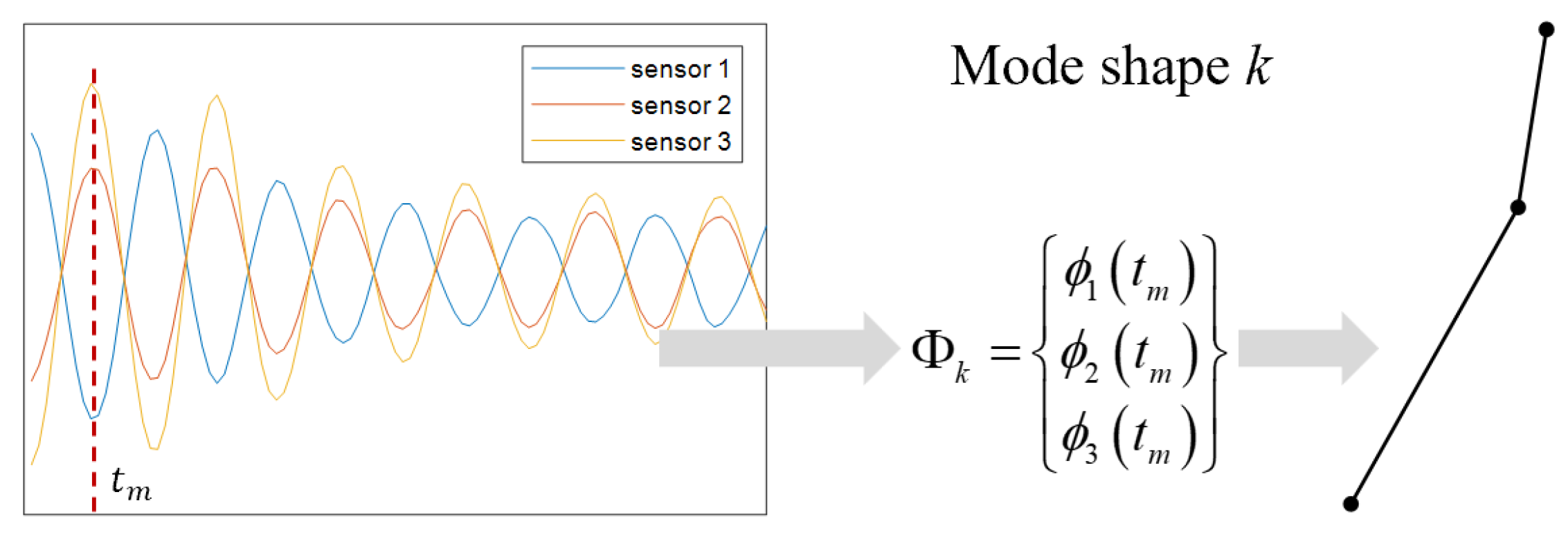
Figure 3.
Flowchart of response surface-based FE model updating.
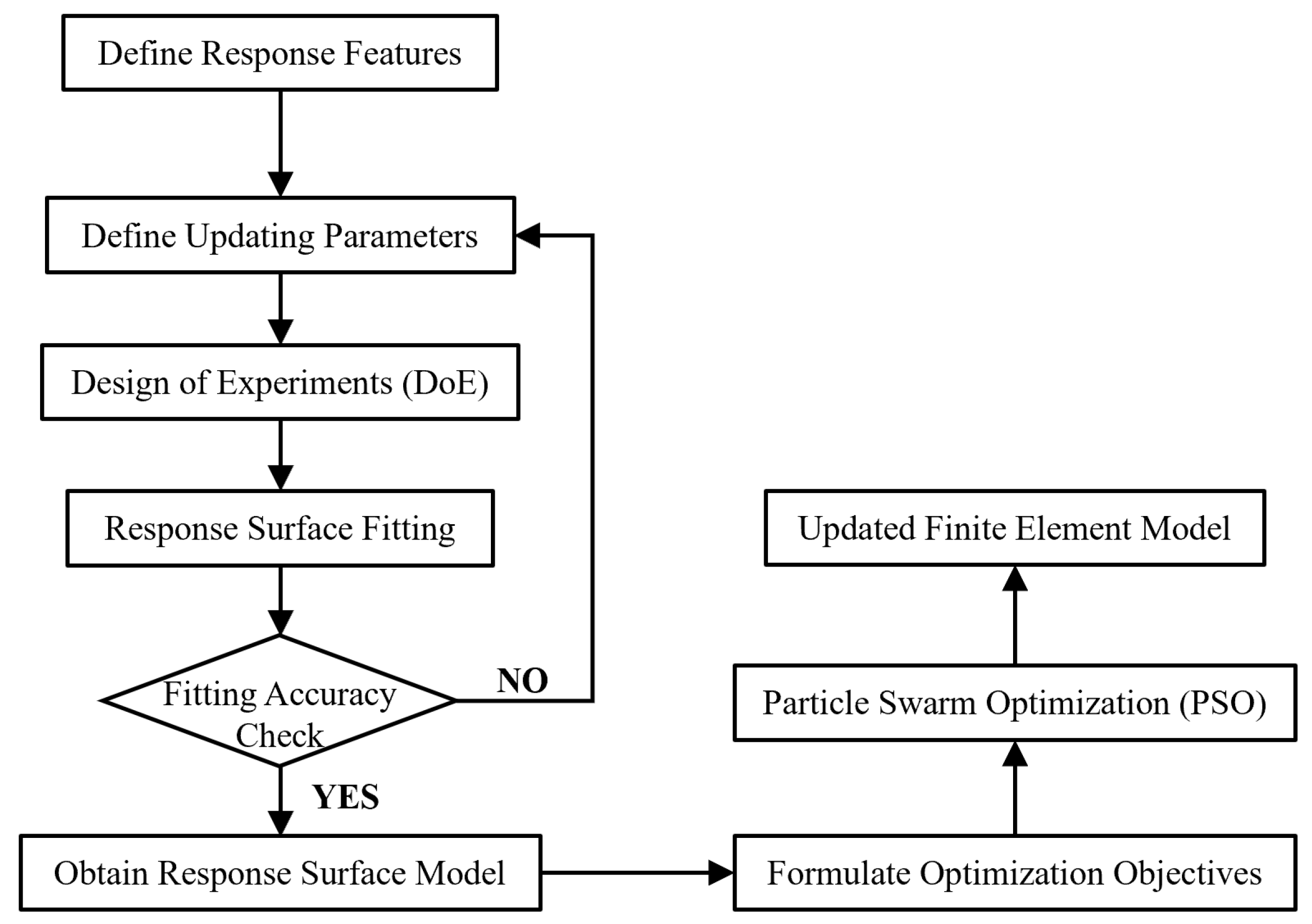
Figure 4.
Flexible PV support structure.
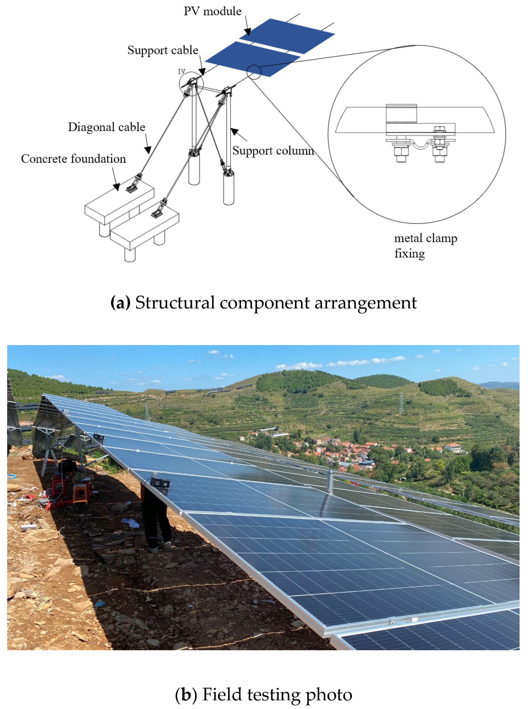
Figure 5.
FE model of the PV support structure.
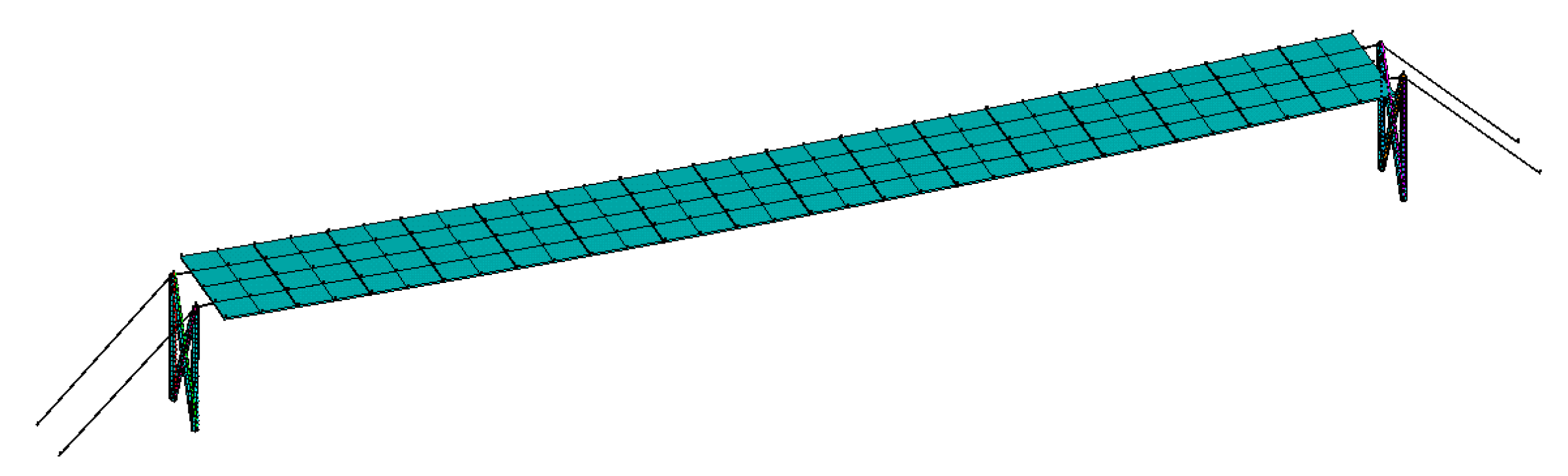
Figure 6.
The first four mode shapes of the PV support structure.
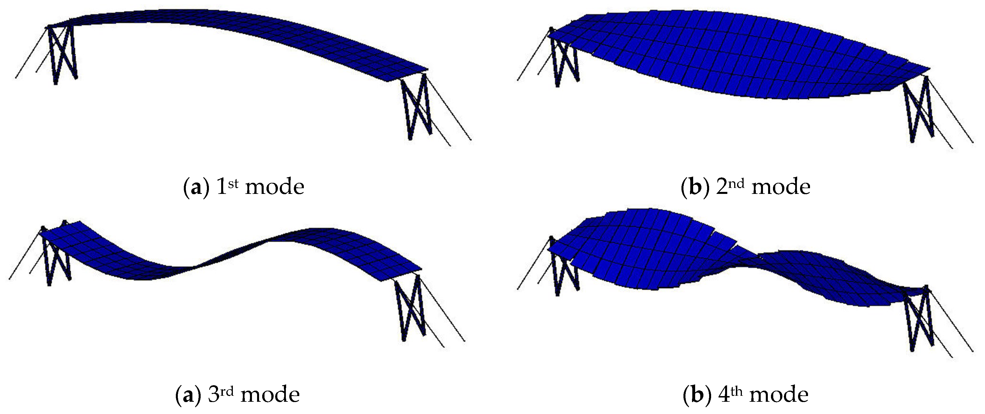
Figure 7.
Attachment of the paper markers and velocity sensors to the PV support structure.
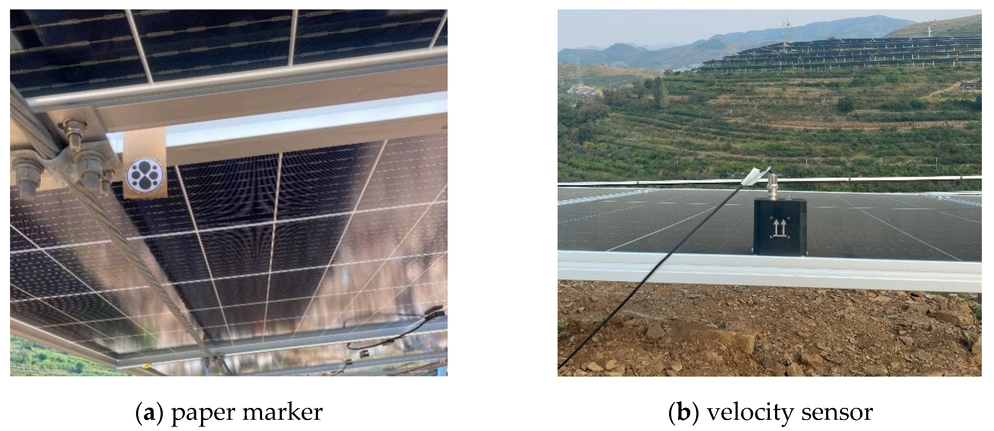
Figure 8.
Sensor placements.
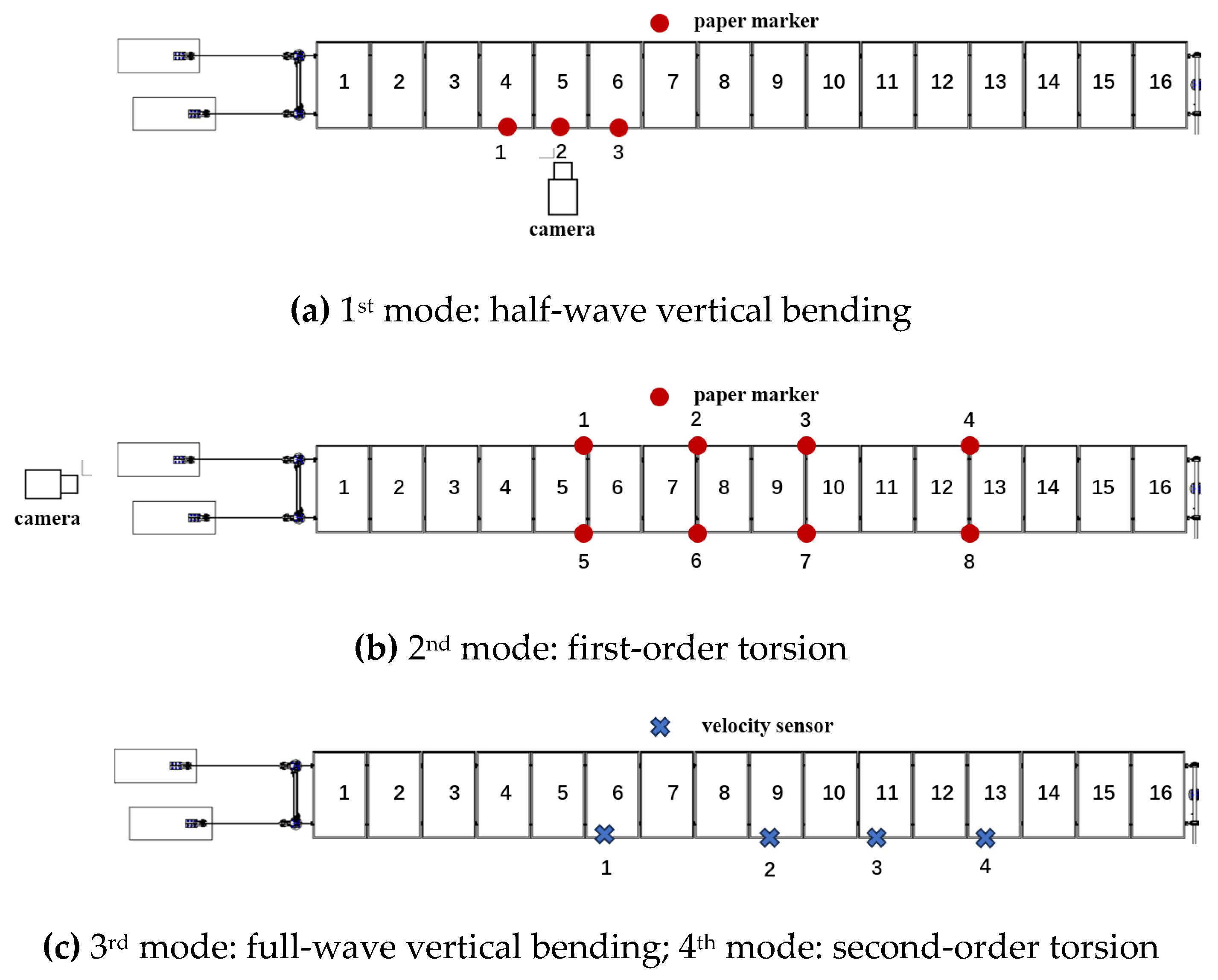
Figure 9.
Camera view.
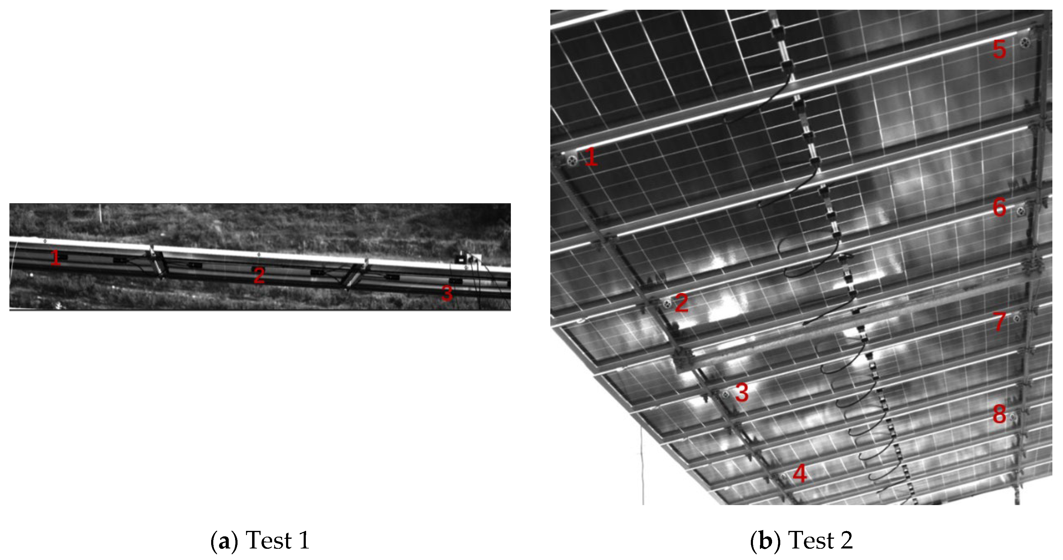
Figure 10.
Time history and spectra of test 1 to test 4.
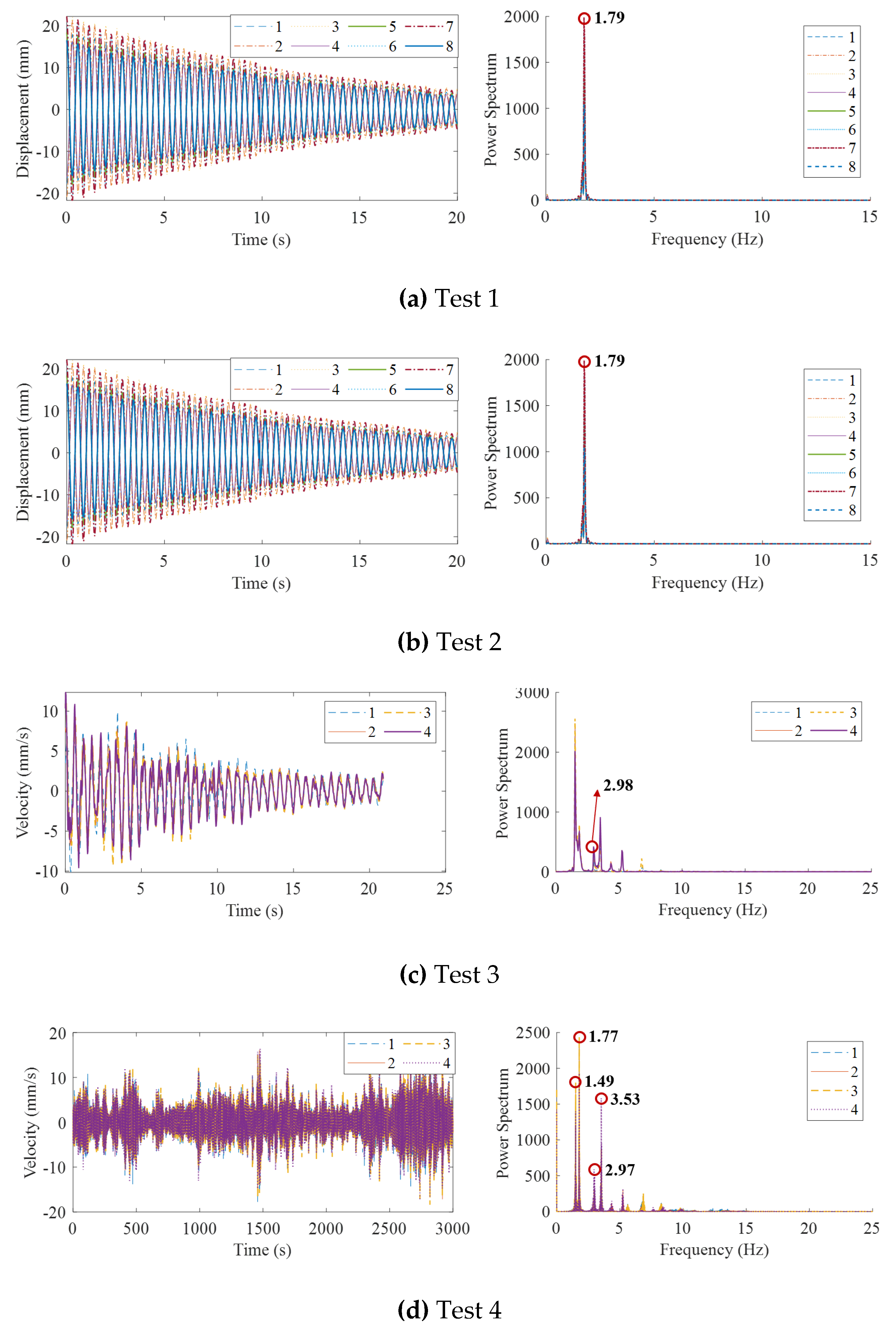
Figure 11.
Time history and spectrum of test 4.
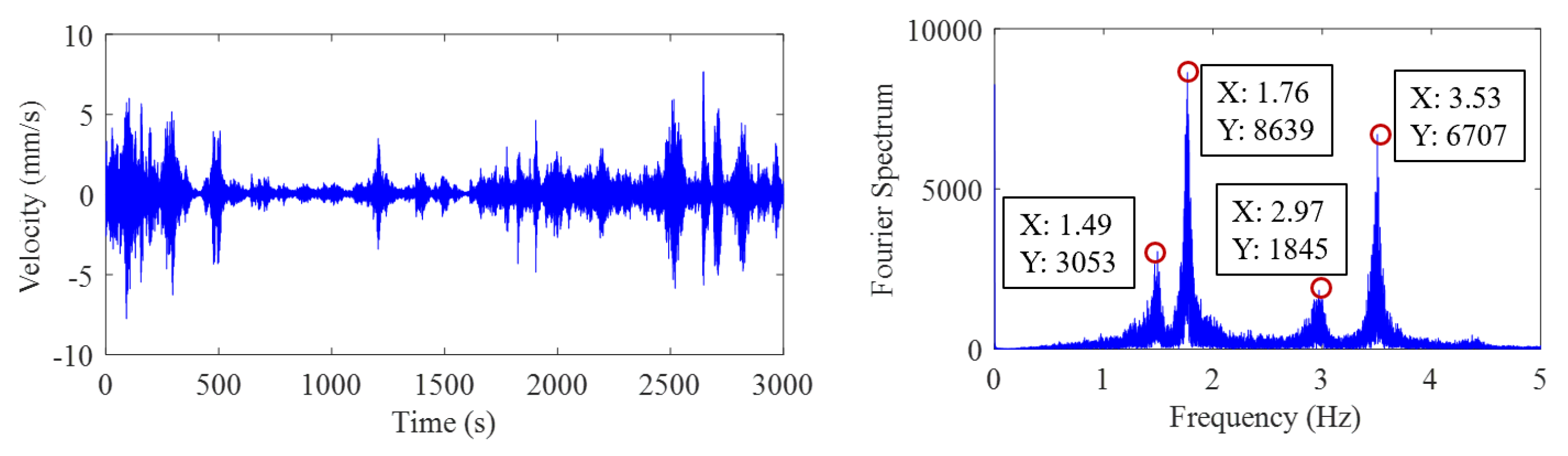
Figure 12.
Time history and spectrum of derived components by the VMD for test 4.
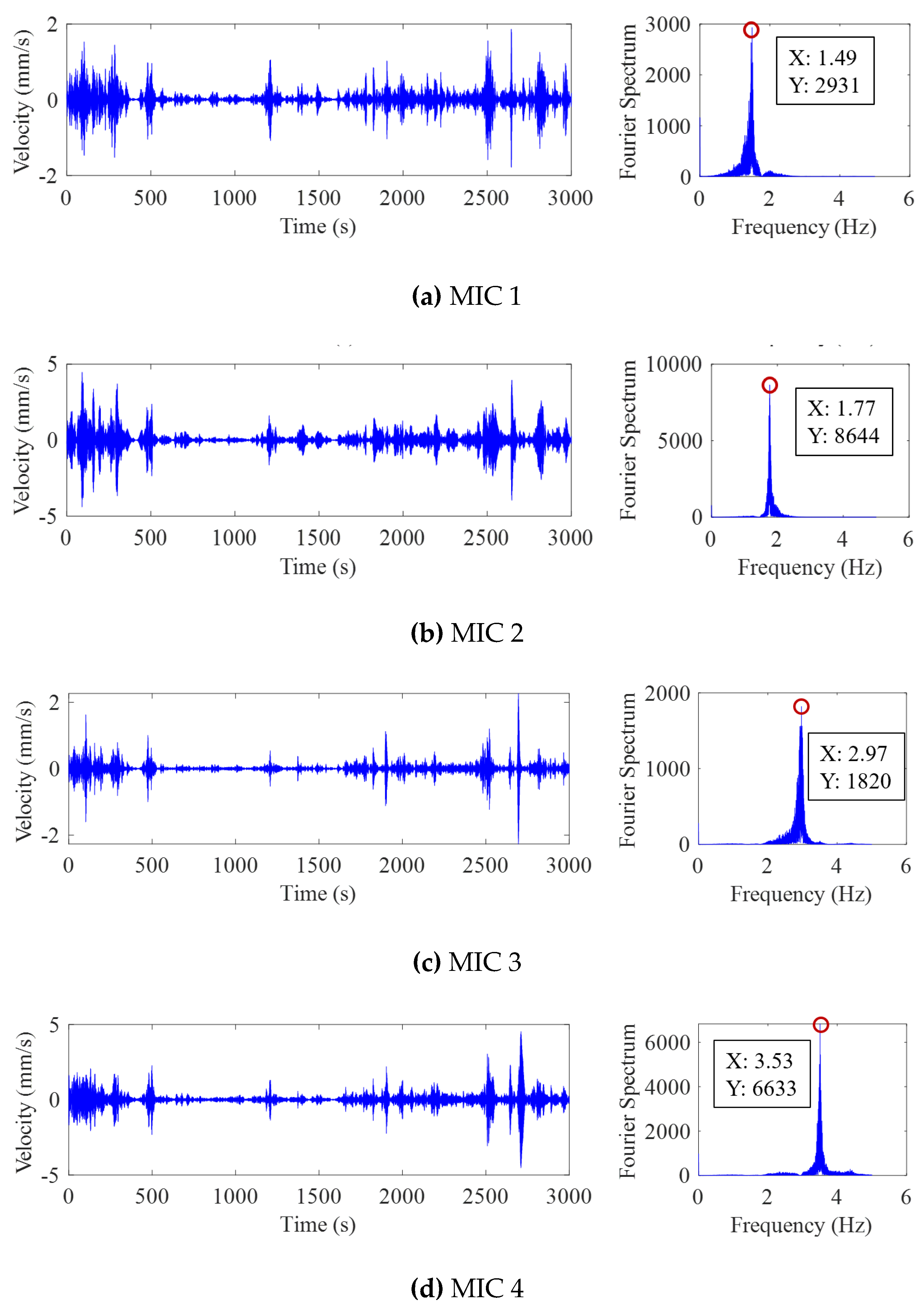
Figure 13.
Second-order torsional spatial mode shape.
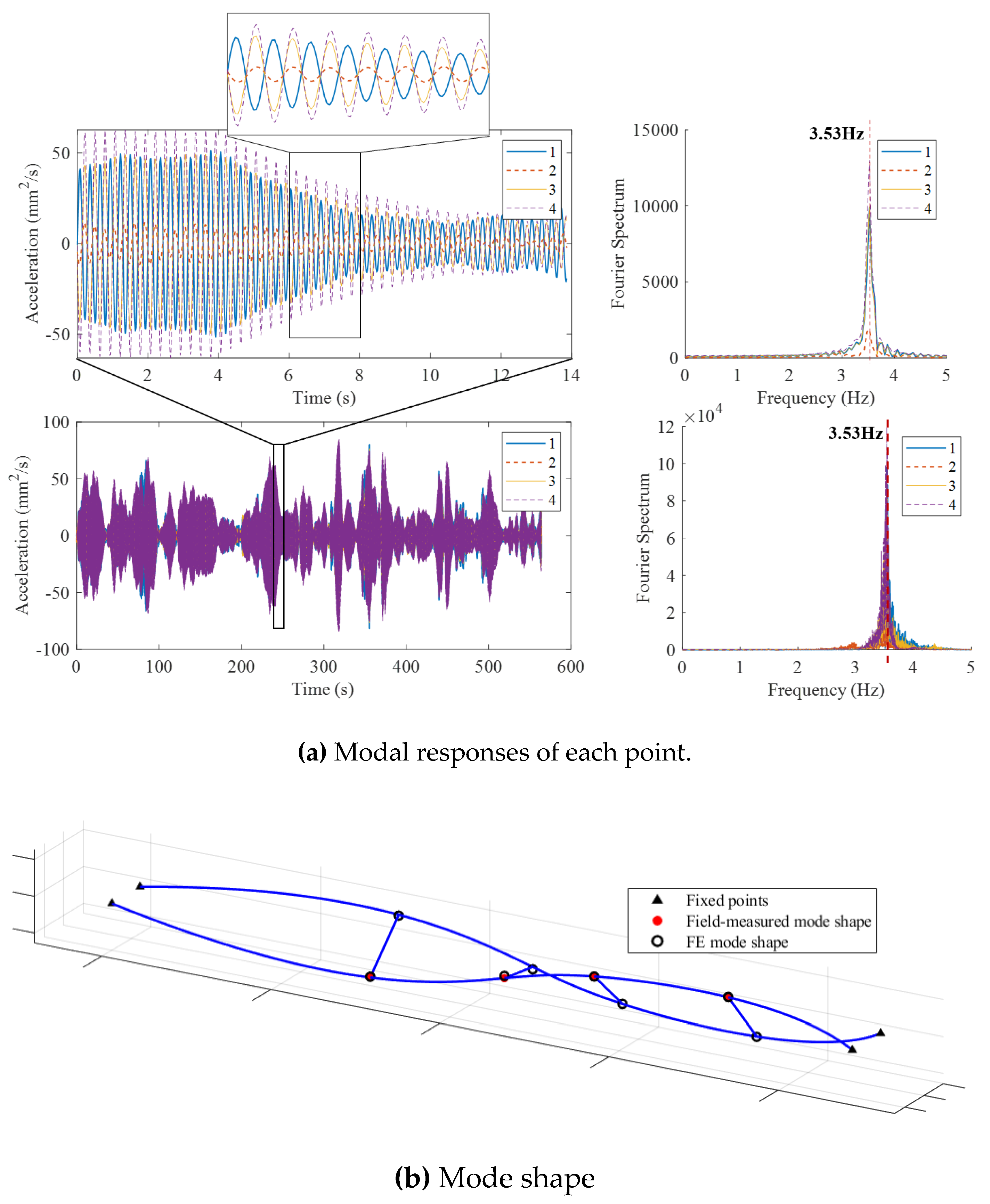
Figure 14.
Half-wave vertical bending mode shape.
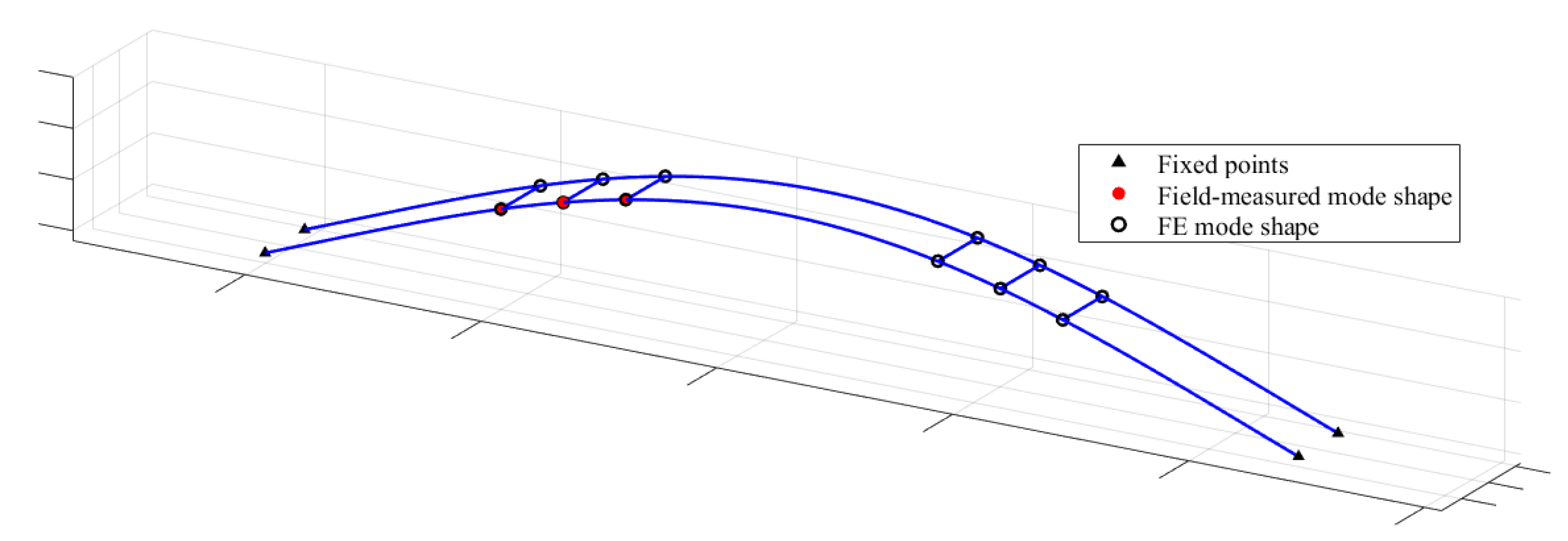
Figure 15.
First-order torsional spatial mode shape.
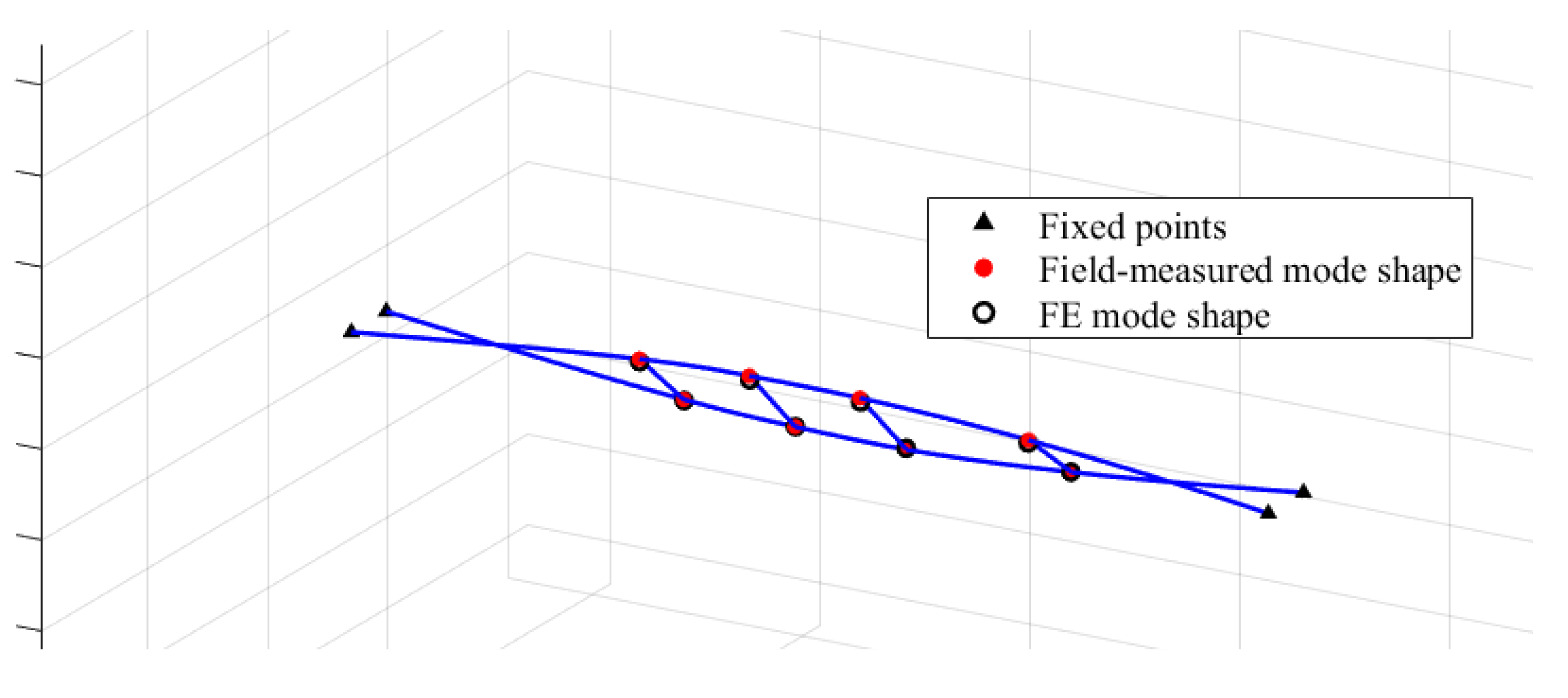
Figure 16.
Full-wave vertical bending mode shape.
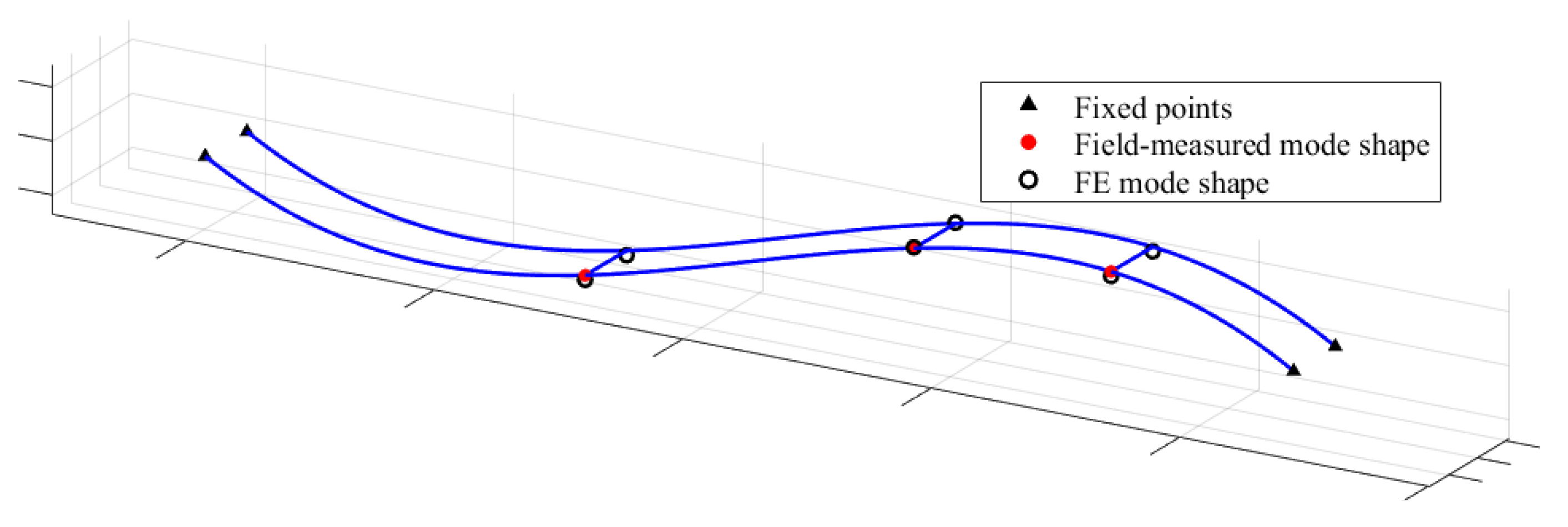
Figure 17.
Response surface fitting results.
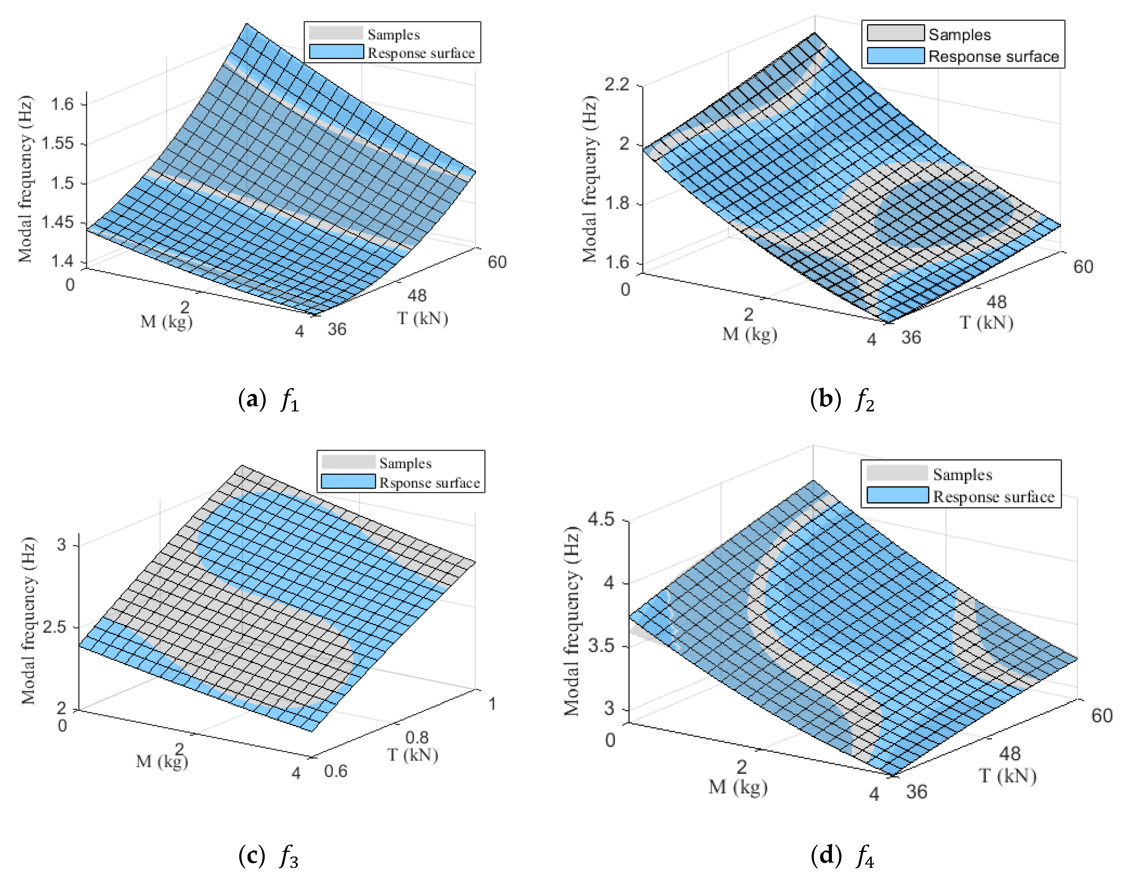
Figure 18.
Convergence curve of the objective function.
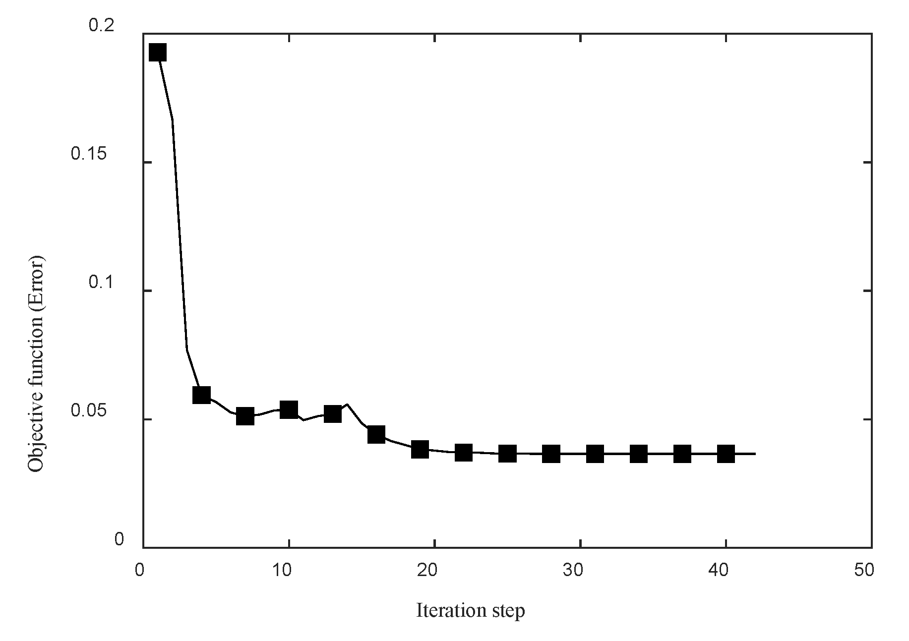
Table 1.
Summary of the test cases.
| Test cases | Target mode | Excitation method | Sensor type | Placement method | Test duration |
|---|---|---|---|---|---|
| 1 | half-wave vertical bending | 1/2 span, vertical harmonic loads | Vison-based measurement | Fig. 5(a) | 5 min |
| 2 | first-order torsion | 1/2 span, vertical synchronized opposite-direction harmonic loads | Vison-based measurement | Fig. 5(b) | 5 min |
| 3 | full-wave vertical bending | 1/4 and 3/4 span, vertical synchronized opposite-direction harmonic loads | Velocity sensor | Fig. 5(c) | 5 min |
| 4 | second-order torsion | Wind excitation | Velocity sensor | Fig. 5(c) | 120 min |
Table 2.
Identified frequencies and damping ratios.
| mode | by SH | by HT | |
|---|---|---|---|
| 1 | 1.488 | 0.0172 | 0.0155 |
| 2 | 1.775 | 0.0065 | 0.0071 |
| 3 | 2.980 | 0.0098 | 0.013 |
| 4 | 3.526 | 0.0035 | 0.0043 |
Table 3.
Comparison of mode shapes from field identification and FE model.
| Mode | Method | Mode shape vector | 1-MAC | |||||||
| 1 | 2 | 3 | 4 | 5 | 6 | 7 | 8 | |||
| 1 | Field- measured |
0.73 | 0.88 | 1 | / | / | / | / | / | 3.33×10⁻⁶ |
| FEM | 0.72 | 0.88 | 1 | / | / | / | / | / | ||
| 2 | Field- measured |
0.88 | 1 | 0.99 | 0.74 | -0.88 | -1 | -0.99 | -0.74 | 8.38×10⁻⁵ |
| FEM | 0.86 | 1 | 1 | 0.73 | -0.86 | -0.1 | -0.99 | -0.73 | ||
| 3 | Field- measured |
0.69 | / | -0.75 | 1 | / | / | / | / | 5.18×10⁻² |
| FEM | 0.82 | / | -0.82 | 1 | / | / | / | / | ||
| 4 | Field- measured |
0.83 | 0.15 | -0.79 | 1 | / | / | / | / | 3.41×10⁻² |
| FEM | 0.79 | 0.18 | -0.79 | 1 | / | / | / | / | ||
Table 4.
Comparison of field-measured and FE analysis modal frequencies.
| Response features | Modal frequencies (Hz) | Relative error (%) | |
|---|---|---|---|
| FE | Field-measured | ||
| f1 | 1.693 | 1.488 | 13.78 |
| f2 | 2.205 | 1.775 | 24.22 |
| f3 | 3.081 | 2.980 | 3.38 |
| f4 | 4.242 | 3.526 | 20.31 |
Table 5.
Range of updating parameter values.
| Updating parameters | Initial value | Lower bound | Upper bound |
|---|---|---|---|
| (kN) | 60 | 36 | 60 |
| (kg) | 0 | 0 | 4 |
| 0 | 0 | 1 |
Table 6.
Fitting validation.
| Index | f1 | f2 | f3 | f4 |
|---|---|---|---|---|
| R2 | 0.998 | 1.000 | 1.000 | 0.998 |
| RMSE | 2.10×10⁻³ | 2.00×10⁻³ | 5.79×10⁻⁴ | 1.230×10⁻² |
Table 7.
Optimization results of updating parameters.
| Updating parameter | Initial | Optimization |
|---|---|---|
| (kg) | 0 | 2.00 |
| (kN) | 60 | 51.96 |
Disclaimer/Publisher’s Note: The statements, opinions and data contained in all publications are solely those of the individual author(s) and contributor(s) and not of MDPI and/or the editor(s). MDPI and/or the editor(s) disclaim responsibility for any injury to people or property resulting from any ideas, methods, instructions or products referred to in the content. |
© 2025 by the authors. Licensee MDPI, Basel, Switzerland. This article is an open access article distributed under the terms and conditions of the Creative Commons Attribution (CC BY) license (http://creativecommons.org/licenses/by/4.0/).
Copyright: This open access article is published under a Creative Commons CC BY 4.0 license, which permit the free download, distribution, and reuse, provided that the author and preprint are cited in any reuse.


